Hostname: page-component-cd9895bd7-7cvxr Total loading time: 0 Render date: 2024-12-23T19:09:25.407Z Has data issue: false hasContentIssue false

Outer scaling of the mean momentum equation for turbulent boundary layers under adverse pressure gradient

Published online by Cambridge University Press:  28 February 2023

Tie Wei*
Affiliation:
Department of Mechanical Engineering, New Mexico Tech, Socorro, NM 87801, USA
Tobias Knopp
Affiliation:
Institute of Aerodynamics and Flow Technology, DLR (German Aerospace Center), Bunsenstr. 10, 37073 Gottingen, Germany
*
Email address for correspondence: tie.wei@nmt.edu

Abstract

A new scaling of the mean momentum equation is developed for the outer region of turbulent boundary layers (TBLs) under adverse pressure gradient (APG). The maximum Reynolds shear stress location, denoted as $y_{m}$, is employed to determine the proper scales for the outer region of an APG TBL. An outer length scale is proposed as $\delta _e - y_{m}$, where $\delta _e$ is the boundary layer thickness. An outer velocity scale for the mean streamwise velocity deficit is proposed as $U_e - U_{m}$, where $U_e$ and $U_m$ are the mean streamwise velocities at the boundary layer edge and $y_{m}$, respectively. An outer velocity scale for the mean wall-normal velocity deficit is proposed as $V_e - V_{m}$, where $V_e$ and $V_{m}$ are the wall-normal velocities at $\delta _e$ and $y_{m}$, respectively. The maximum Reynolds shear stress is found to scale as $(\delta _e - y_{m}) U_e \,{\rm d}U_e/{{\rm d}x}$. The new outer scaling collapses well the experimental and numerical data on APG TBLs over a wide range of Reynolds numbers and strengths of pressure gradient. Approximations of the new scaling are developed for TBLs under strong APG and at high Reynolds numbers. The relationships between the new scales and previously proposed scales are discussed.

Type
JFM Papers
Copyright
© The Author(s), 2023. Published by Cambridge University Press

1. Introduction

Turbulent boundary layer (TBL) flows subject to an adverse pressure gradient (APG) often play a critical role in determining the performance of a variety of engineering devices. Under a strong APG, the boundary layer flow may separate from the solid surface, causing a drastic change in the flow pattern. Therefore, accurate knowledge of the development of the APG boundary layer is pivotal in predicting the overall performance of the device, e.g. for the wing design of modern aircraft (Slotnick & Heller Reference Slotnick and Heller2019).

APG TBLs have been the subject of numerous theoretical, experimental and numerical studies. The scaling of the outer layer of a TBL was first developed from the velocity-defect law formulation by von Kármán (Reference von Kármán1930) and Millikan (Reference Millikan1938). In the outer region, where viscous effects are not important, the scaling is applied to the mean velocity defect $U_{e}-U$ compared to the boundary layer edge mean velocity $U_{e}$. For the zero pressure gradient (ZPG) case, the classical velocity scale is the wall friction velocity $u_\tau$, and the classical length scale is the defect displacement thickness $\varDelta$, known as the Rotta–Clauser length scale (Rotta Reference Rotta1950; Clauser Reference Clauser1954):

(1.1)\begin{equation} \frac{U_{e}-U}{u_\tau}= g\left(\frac{y}{\varDelta}\right). \end{equation}

The Rotta–Clauser parameter $\beta _{RC} = (\delta ^*/(\rho u^2_\tau )) \,{\rm d}P_e/{{\rm d}x}$ is commonly used to characterize the strength of pressure gradient. Here, $\delta ^*$ is the mass displacement thickness. In the case of an APG, the scaling of (1.1) is appropriate for $\beta _{RC}<8$, shape factor $H<1.8$, and the corresponding small mean velocity defect (see Maciel et al. Reference Maciel, Wei, Gungor and Simens2018). For a large defect ($\beta _{RC}>8$, $H>1.8$), the pressure velocity $u_p=(\delta ^* \rho ^{-1} \,\mathrm {d}P_e/\mathrm {d} x)^{1/2}$ of Mellor & Gibson (Reference Mellor and Gibson1966), together with a modified defect displacement thickness, which involves $u_p$ rather than $u_\tau$, can be used. A summary of outer scales used previously is given in table 2 of Maciel et al. (Reference Maciel, Wei, Gungor and Simens2018).

Building on their study of the TBL as a wall-confined wake, Schofield & Perry (Reference Schofield and Perry1972) proposed a velocity scale $U_m$ that is related to the maximum shear stress in the boundary layer $\tau _m$. Denote $U_m=(\tau _m/\rho )^{1/2}$, and let $y_m$ be the wall distance of $\tau _m$. Then the defect law is formulated using the velocity scale $U_s$ and a length scale $B$. The velocity scale $U_s$ is defined by an extrapolation of the half-power law for the mean velocity to the wall, and $U_s$ and $B$ are related to $U_m$ and $y_m$ by the relations $B=2.86\delta ^*U_e/U_s$ and $U_s=8(B/y_m)^{1/2}U_m$ (see Perry & Schofield Reference Perry and Schofield1973; Schofield Reference Schofield1981).

Recently, several alternative outer layer scales have been proposed. In their study of turbulent pipe flows, Zagarola & Smits (Reference Zagarola and Smits1998a) proposed a new outer velocity scale as $U_{ctr} - U_{avg}$, where $U_{ctr}$ is the mean axial velocity at the pipe centreline, and $U_{avg}$ is the bulk velocity. Extending to a ZPG TBL, the Zagarola–Smits outer scale can be written as $U_\infty - U_{avg} = U_\infty \delta ^*/\delta _e$. Zagarola & Smits (Reference Zagarola and Smits1998b) showed that the new velocity scale collapsed the experimental data significantly better than profiles normalized by the friction velocity or free stream velocity. The Zagarola–Smits velocity scale has also been used to collapse APG TBL data.

Gungor et al. (Reference Gungor, Maciel, Simens and Soria2016) proposed an outer velocity scale as twice the velocity deficit at the middle of the shear layer, $2(U_e - U(y=0.5 \delta _e))$, based on the similarity between the outer region of the APG TBL and the single-stream mixing layer. Schatzman & Thomas (Reference Schatzman and Thomas2017) proposed an embedded shear layer scaling. This scaling assumes the existence of an inflection point for the mean velocity profile in the outer layer at the wall distance $y_{IP}$. The inflection point is used as an anchor to define the new scaling. The velocity scale is the local velocity defect at the inflection point, $U_{d}=U_{e}-U_{IP}$, the length scale is the local embedded shear layer vorticity thickness $\delta _\omega$, and the scaled wall distance becomes $(y-y_{IP})/\delta _\omega$. The scaled mean velocity becomes $(U_{e}-U)/U_{d}$.

A similar scaling was proposed by Sekimoto et al. (Reference Sekimoto, Kitsios, Atkinson, Sillero, Borell, Gungor, Jimenez and Soria2019). They consider the shear rate $S$, normalized by a turbulence time scale $k/\epsilon$. Here, $k$ is the turbulent kinetic energy (TKE), and $\epsilon$ is the turbulent dissipation. They define the shear thickness $\delta _s$ as the distance from the wall to the maximum of the quantity $(y/\delta ^*)(S k/\epsilon )$. For the velocity scale, the pressure velocity is redefined as $u_p=(\delta _s \rho ^{-1} \,\mathrm {d}P_e/\mathrm {d} x)^{1/2}$. To this end, a mixed friction–pressure velocity $u^*=(u_\tau ^2+u_p^2(y/\delta _s))^{1/2}$ is defined, which involves the wall distance $y$. A similar velocity scale was proposed by Romero et al. (Reference Romero, Zimmerman, Philip and Klewicki2021).

The modifications of the outer scales summarized above concur with the findings for the balance of the TKE and of the Reynolds stresses. The balance of the TKE is found to be different, however, in TBL flows subjected to an APG. While the peak in the TKE production occurs at approximately $y^+=10\unicode{x2013}20$ in the ZPG case, the peak of TKE production is typically in the outer part of the APG TBL at approximately $y/\delta _e=0.3\unicode{x2013}0.4$. The outer peak of TKE production and turbulence intensity is closely related to an inflection point in the mean velocity profile (see Elsberry et al. Reference Elsberry, Loeffler, Zhou and Wygnanski2000; George, Stanislas & Laval Reference George, Stanislas and Laval2012). According to George et al. (Reference George, Stanislas and Laval2012), an inflectional mean velocity profile forms as a TBL under an APG evolves downstream over a sufficiently long distance, independent of whether the boundary layer ultimately separates. For moderate velocity defects, there is an outer peak of TKE production without the presence of an inflection point in the mean velocity profile. In other words, the peak is not directly related to an inflection point in all cases.

The classical description of the mean velocity profile is based on Coles’ notion that a boundary layer flow can be viewed as a wake-like structure that is constrained by a wall; see Coles & Hirst (Reference Coles and Hirst1969). This is manifested in their famous law-of-the-wall/law-of-the-wake equation:

(1.2a,b)\begin{equation} U^+=\frac{1}{\kappa}\log(y^+) + B + \mathcal{W}(\eta),\quad \mathcal{W}(\eta)=\frac{2\varPi}{\kappa}\left(\sin\left(\frac{{\rm \pi}\eta}{2}\right)\right)^2, \end{equation}

where $y^+= y u_\tau /\nu$ is the inner scaled distance from the wall, and $\eta =y/\delta$ is the outer scaled distance from the wall. In more recent work, modified forms $\mathcal {W}(\eta )=b(1-\exp (p(\eta ))$ with a suitable polynomial $p(\eta )$ have been used for the wake function (see Nickels Reference Nickels2004; Monkewitz, Chauhan & Nagib Reference Monkewitz, Chauhan and Nagib2007). The outer region is influenced by the interaction between turbulence and the free stream at the turbulent/non-turbulent interface (TNTI; Corrsin Reference Corrsin1943; Corrsin & Kistler Reference Corrsin and Kistler1955; Klebanoff Reference Klebanoff1955). In this vein, an alternative view of the outer part of the TBL was given by Krug, Philip & Marusic (Reference Krug, Philip and Marusic2017). They devise a two-state model, consisting of an inertial self-similar region designated as pure wall flow state (featuring a log-law velocity distribution) and the free stream state together with a stochastic model at the interface. Their physical interpretation of the two-state model is to lump the effects of internal shear layers and the TNTI into a single discontinuity at the interface.

Regarding the Reynolds stresses, Kitsios et al. (Reference Kitsios, Atkinson, Sillero, Borell, Gungor, Jimenez and Soria2016) report collapse of the normal stresses scaled by $U_e^2$ and of the shear stress $-\overline {u'v'}$ scaled by $U_e^2 \, \mathrm {d}\delta ^*/\mathrm {d} x$ plotted versus $y/\delta ^*$. However, such a collapse was not found in the study of Bobke et al. (Reference Bobke, Vinuesa, Örlü and Schlatter2017). Elsberry et al. (Reference Elsberry, Loeffler, Zhou and Wygnanski2000) found that a mixed scaling $U_eU_0$ (with a constant reference velocity $U_0$ independent of $x$) produces near-collapse of $-\overline {u'v'}$ for their experimental data.

A new outer scaling of the mean momentum equation for an APG TBL is developed in the present work using the scaling patch approach, which was originally developed to investigate the multi-layer and multi-scaling properties of turbulent pipe or channel flows (see Fife et al. Reference Fife, Klewicki, McMurtry and Wei2005; Wei et al. Reference Wei, Fife, Klewicki and McMurtry2005; Fife Reference Fife2006; Fife, Klewicki & Wei Reference Fife, Klewicki and Wei2009; Wei Reference Wei2020). The scaling patch approach has been applied successfully to rough-wall TBLs (Mehdi, Klewicki & White Reference Mehdi, Klewicki and White2010), turbulent channel flow with heat transfer (Zhou, Pirozzoli & Klewicki Reference Zhou, Pirozzoli and Klewicki2017), buoyancy-driven turbulent convection (Wei Reference Wei2019), and more recently free shear turbulent flows, including jets, wakes and mixing layers (Wei & Livescu Reference Wei and Livescu2021a,Reference Wei and Livescub; Wei, Livescu & Liu Reference Wei, Livescu and Liu2022b; Wei, Li & Livescu Reference Wei, Li and Livescu2022a). Whereas some concepts and ideas in the scaling patch approach are similar to previous scaling approaches, the logical train of thought in the new approach is distinctly different (Fife Reference Fife2006; Wei Reference Wei2020).

One objective of a scaling patch analysis is to reveal naturally the relative magnitudes of different terms in an engineering equation. Such an equation typically consists of more than two terms, with the terms contributing unequally to the balance of the equation. The relative magnitude of each term is often not obvious when the equation is presented in a dimensional form. Through a systematic transformation of the dimensional equation into a dimensionless form, the scaling patch approach is able to determine the scales for the various terms (Fife Reference Fife2006; Wei Reference Wei2020). A key component of the approach is to formulate an admissible scaling for the governing equation. The admissible scaling equation will be a dimensionless equation in which at least two pre-factors of the terms in the equation have nominal order 1, and the other pre-factors have nominal order either 1 or 0. Moreover, the dimensionless boundary conditions should also be $0$ or nominal order 1.

In § 2, the scaling patch approach is applied to develop the new outer scaling equation, and new outer scales for the length, velocity and Reynolds shear stress are proposed. The new scaling is verified against experimental and numerical data in § 3. Approximate outer scales are presented in § 4. In § 5, the relationship between the new scales and the results of previous analysis are presented. Section 6 summarizes the work.

2. New outer scaling for the mean momentum equation in APG TBL

Due to its significance in understanding and modelling of turbulent flows, the Reynolds shear stress distribution has been a major focus in turbulence research. In a TBL over a flat plate (ZPG TBL) or turbulent flow through a pipe or channel, it is known (see e.g. Long & Chen Reference Long and Chen1981; Afzal Reference Afzal1982; Sreenivasan & Sahay Reference Sreenivasan and Sahay1997; Wei et al. Reference Wei, Fife, Klewicki and McMurtry2005) that the location of maximum Reynolds shear stress $y_{m}$ is proportional to the geometric mean of the inner length scale $\nu /u_\tau$ and the outer scale $\delta _e$: $y_{m} \propto \sqrt {\nu /u_\tau \delta _e}$. At high Reynolds numbers, $y_{m}$ is a small fraction of $\delta _e$. That is, the maximum Reynolds shear stress location is close to the wall in the ZPG TBL. For instance, at ${Re}_\tau = \delta _e u_\tau /\nu =1000$, $y_{m}/\delta _e \sim 0.03$, and at ${Re}_\tau = 5000$, $y_{m}/\delta _e \sim 0.01$.

Under an APG, however, the location of the maximum Reynolds shear stress in TBLs shifts outwards. For example, a value $y_{m} \approx 0.4 \delta _e$ was found for the equilibrium TBL under a strong APG in Skåre & Krogstad (Reference Skåre and Krogstad1994), as shown in figure 1. In the present work, the characteristics of the Reynolds shear stress distribution are employed to determine the proper scales for the flow in the outer region of the APG TBL.

Figure 1. Defining the new outer scales for an APG TBL. The data are from experiments of Skåre & Krogstad (Reference Skåre and Krogstad1994) at the sixth station (${Re}_\tau \approx 5160$ and $\beta _{RC}=21.2$). The sketch is to illustrate the shapes of the profiles; the magnitudes on the vertical axis do not scale.

The governing equations for a statistically steady two-dimensional TBL under pressure gradient are (see e.g. Tennekes & Lumley Reference Tennekes and Lumley1972)

(2.1a)\begin{gather} 0 = \frac{\partial U}{\partial x} + \frac{\partial V}{\partial y}, \end{gather}
(2.1b)\begin{gather}0 ={-}U\,\frac{\partial U}{\partial x} - V\,\frac{\partial U}{\partial y}+ \frac{\partial R_{uv}}{\partial y} + \frac{\partial (R_{uu}-R_{vv})}{\partial x}- \frac{1}{\rho}\,\frac{{\rm d} P_e}{{\rm d} x} + \nu\,\frac{\partial^2 U }{\partial y^2}. \end{gather}

Here, upper-case letters $U$ and $V$ denote the mean velocity component in the streamwise $x$-direction and wall-normal $y$-direction, respectively, and $P_e$ is the mean pressure in the free stream. Fluid density is $\rho$. The kinematic Reynolds shear stress is denoted as $R_{uv} = - \langle u v \rangle$, where lower-case letters $u$ and $v$ are the velocity fluctuations in the streamwise and wall-normal directions, respectively, and angle brackets denote Reynolds averaging. The Reynolds normal stresses in the streamwise and wall-normal directions are denoted as $R_{uu}=-\langle u u \rangle$ and $R_{vv} = -\langle vv \rangle$, respectively. In the outer region of APG TBL, viscosity has a negligible effect on the flow, and the viscous term in (2.1b) will be neglected in the following analysis. In general, the turbulence term $\partial (R_{uu}-R_{vv})/\partial x$ also has a negligible effect on the balance of the mean momentum equation (2.1b), and is omitted in the following analysis (Townsend Reference Townsend1956). The flow conditions at $y_m$ and $\delta _e$ are listed in table 1. In the present work, the boundary layer edge is determined as the location of 1 % $|R_{uv}|_{max}$ if the data points of Reynolds shear stress data are spaced closely in the wall-normal direction. If the data points of Reynolds shear stress are not spaced closely, then the location of 5 % $|R_{uv}|_{max}$ is used to determine the boundary layer edge. Compared with the mean streamwise velocity profile, it is more robust and easier to determine the boundary layer edge using the Reynolds shear stress profile. Furthermore, the new determination of $\delta _e$ is applicable to both TBL flows and free shear flows (wake flow, planar mixing layer), indicating the close connection between the outer region of the APG TBL and planar turbulent mixing layers discussed in § 3.

Table 1. Conditions at the maximum Reynolds shear stress location $y_{m}$ and boundary layer edge $\delta _e$.

The first step of the scaling patch approach is to construct the scaled variables (denoted by a superscript $^*$), whenever possible, to vary between $0$ and $1$. Such a scaled variable is able to reveal a natural reference scale for the flow variable. The scaled wall-normal location and flow variables are

(2.2a)\begin{gather} y^* \mathop{=}\limits^{{\rm def}} \frac{y-y_{m}}{y_{ref}(x)}, \end{gather}
(2.2b)\begin{gather}U^* \mathop{=}\limits^{{\rm def}} \frac{U_e - U}{U_{ref}(x)}, \end{gather}
(2.2c)\begin{gather}V^* \mathop{=}\limits^{{\rm def}} \frac{V_e - V}{V_{ref}(x)}, \end{gather}
(2.2d)\begin{gather}R^*_{uv} \mathop{=}\limits^{{\rm def}} \frac{R_{uv}}{R_{uv,{ref}}(x)}. \end{gather}

The reference scales $y_{ref}$, $U_{ref}$, $V_{ref}$ and $R_{uv,{ref}}$ depend on $x$ only. Note that self-similarity is not assumed in the definition of $U^*$, $V^*$ and $R^*_{uv}$. That is, the scaled variables $U^*$, $V^*$ and $R^*_{uv}$ may vary in both $y^*$ and $x$. The scaling wall-normal location $y^*$ deserves some comment. It uses the well-known finding from APG TBL that an outer maximum of the turbulent shear stress appears at a wall distance $y_m$. As the derivative $\partial R_{uv}/\partial y$ enters into the mean momentum balance (2.1b), it appears natural to use $y_m$ as an anchor point for $y^*$.

In previous similarity analyses of APG TBL, the mean streamwise velocity deficit $U_e-U$ was used typically, but the wall-normal velocity was used directly. Here, the wall-normal velocity deficit is used in the scaled variable to remove the wall effect in the outer region. As pointed out by Castillo & George (Reference Castillo and George2001), there is no need to use a deficit to define the normalized Reynolds shear stress, because the Reynolds shear stress is approximately zero at the boundary layer edge, so $R_{uv}|_e - R_{uv} \approx - R_{uv}$.

Substituting the normalized variables defined in (2.2a)–(2.2d) into the mean momentum equation (2.1b) produces

(2.3)\begin{align} 0 & ={-} \frac{U_e V_{ref}}{y_{ref}}\,\frac{\partial V^*}{\partial y^*} + \frac{U_{ref} V_e}{y_{ref}}\,\frac{\partial U^*}{\partial y^*} + \frac{U_{ref} V_{ref}}{y_{ref}} \left( U^*\,\frac{\partial V^*}{\partial y^*} - V^*\,\frac{\partial U^*}{\partial y^*} \right) \nonumber\\ &\quad + \frac{R_{uv,{ref}}}{y_{ref}}\,\frac{\partial R^*_{uv}}{\partial y^*} - \frac{1}{\rho}\,\frac{{\rm d} P_e}{{\rm d} x}. \end{align}

Note that the continuity equation (2.1a) is employed to write $-U\,\partial U/\partial x$ as $U\,\partial V/\partial y$ in the mean momentum equation, so there is no $x$ derivative in (2.3) except in ${\rm d}P_e/{{\rm d} x}$. The flow conditions at $y=y_{m}$ and $y=\delta _e$ for the normalized variables are listed in table 2. To satisfy the admissible scaling requirement for the boundary conditions (see Fife Reference Fife2006; Wei Reference Wei2020), proper scales for $y_{ref}$, $U_{ref}$ and $V_{ref}$ are set as

(2.4a)\begin{gather} y_{ref} = \delta_e - y_{m}, \end{gather}
(2.4b)\begin{gather}U_{ref} = U_e - U_{m}, \end{gather}
(2.4c)\begin{gather}V_{ref} = V_e - V_{m}, \end{gather}
(2.4d)\begin{gather}R_{uv,{ref}} = R_{uv}|_{max}. \end{gather}

Consequently, all the normalized boundary conditions at $y^*=0$ (at $y=y_{m}$) and $y^*=1$ (at $y=\delta _e$) are either 1 or 0. Therefore, in the outer region of the APG TBL, the scaled variables $U^*$, $V^*$ and $R^*_{uv}$ in the scaling patch analysis all vary between $0$ and $1$ within the scaled distance of $0 \leqslant y^* \leqslant 1$. Moreover, as $U^*$, $V^*$ and $R^*_{uv}$ are smooth functions of $y^*$ in the outer region, their derivatives $\partial /\partial y^*$ and $\partial ^2/\partial (y^*)^2$ also remain $\leqslant O(1)$.

Table 2. Conditions at $y_{m}$ and $\delta _e$.

The mean momentum equation in a dimensionless form can be obtained by dividing $U_e \,{\rm d}U_e/{{\rm d} x}$ into (2.3):

(2.5)\begin{align} 0 & ={-} \left[ \frac{V_e-V_{m}}{(\delta_e-y_{m})\,\dfrac{{\rm d}U_e}{{\rm d} x}} \right] \frac{\partial V^*}{\partial y^*} + \left[ \frac{U_e-U_{m}}{U_e}\,\frac{V_e}{(\delta_e-y_{m})\,\dfrac{{\rm d}U_e}{{\rm d} x}} \right] \frac{\partial U^*}{\partial y^*} \nonumber\\ &\quad + \left[ \frac{U_e-U_{m}}{U_e}\, \frac{V_e-V_{m}}{(\delta_e-y_{m})\,\dfrac{{\rm d}U_e}{{\rm d} x}} \right] \left( U^*\,\frac{\partial V^*}{\partial y^*} - V^*\,\frac{\partial U^*}{\partial y^*}\right) \nonumber\\ &\quad + \left[ \frac{R_{uv}|_{max}}{(\delta_e-y_{m}) U_e\,\dfrac{{\rm d}U_e}{{\rm d} x}} \right] \frac{\partial R^*_{uv}}{\partial y^*} - \frac{\dfrac{1}{\rho}\, \dfrac{{\rm d} P_e}{{\rm d} x}}{U_e\,\dfrac{{\rm d}U_e}{{\rm d} x}}. \end{align}

Note that the last term in (2.5) is 1, as $-(1/\rho )\,{\rm d}P_e/{{\rm d} x} = U_e \,{\rm d}U_e/{{\rm d} x}$ from the mean momentum equation in the free stream. If there is at least another pre-factor in (2.5) (in the square brackets) having nominal order 1, then this equation satisfies the requirement for an admissible scaling. The variations of the pre-factors in the $x$-direction are presented in figure 2. The pre-factor of the first term in (2.5), $(V_e -V_{m})/((\delta _e - y_{m}) \,{\rm d}U_e/{{\rm d} x})$, approaches a constant $-2.5$, which is of $o(1)$. The deviation at the beginning of the simulation domain is attributed to the fact that the APG effect takes some distance to influence the outer flow in the boundary layer. Figure 2(b) shows that $(U_e - U_{m})/U_e$ approaches a constant of value $0.3\unicode{x2013}0.4$. Hence the pre-factor of the third term in (2.5) also approaches a constant in the range $-0.75$ to $-1.0$. Figure 2(c) shows that $V_e/((\delta _e - y_{m})\,{\rm d}U_e/{{\rm d} x})$ can be approximated by a constant $-3$. (The cause of the scatter and rise near the end of the simulation domain in figure 2(c) is not clear to the authors.) Therefore, the pre-factor of the second term in (2.5) is in the range $-0.9$ to $- 1.2$. Figure 2(d) shows that the pre-factor of the fourth term in (2.5) varies between $-0.5$ and $-0.6$, except near the beginning and end of the large-eddy simulations (LES) domain. Note that the LES studies of Bobke et al. (Reference Bobke, Vinuesa, Örlü and Schlatter2017) were on near-equilibrium mild APG TBLs. At present, it is not clear whether the values presented in figure 2 vary with the streamwise distribution of the pressure gradient and strength of APG, especially for flow near the separation. More studies are required to look into the issue.

Figure 2. Parameters in the pre-factors of (2.5). (a) Pre-factor of the first term in (2.5). (b) Plots of $(U_e-U_{m})/U_e$ versus $x$. (c) Plots of $V_e/((\delta _e-y_{m})\,{\rm d}U_e/{{\rm d} x})$ versus $x$. (d) Pre-factor of Reynolds shear stress gradient term in (2.5). The LES data are from Bobke et al. (Reference Bobke, Vinuesa, Örlü and Schlatter2017), and the DNS data are from Kitsios et al. (Reference Kitsios, Sekimoto, Atkinson, Sillero, Borrell, Gungor, Jiménez and Soria2017). To prevent clutter, only every $80$ $x$-grids are plotted.

The values of the pre-factors of terms in (2.5) are summarized in table 3 based on the LES of Bobke et al. (Reference Bobke, Vinuesa, Örlü and Schlatter2017), showing that all the pre-factors in (2.5) are constants of nominal order $1$. In other words, (2.5) is an admissible scaling of the mean momentum equation for the outer region of the APG TBL.

Table 3. Values of the pre-factors of terms in (2.5), computed from the LES data of Bobke et al. (Reference Bobke, Vinuesa, Örlü and Schlatter2017).

3. Evaluating the new outer scales using experimental and numerical simulation data

The new outer scaling is evaluated against experimental and numerical simulation data on the APG TBL over a wide range of Reynolds numbers and strengths of the pressure gradient. Table 4 lists the $x$ station (or the grid index in simulation), the momentum thickness Reynolds number $Re_\theta$, the Rotta–Clauser parameter $\beta _{RC}$, and the shape factor $H$ of the data used in this work. Marušić & Perry (Reference Marušić and Perry1995) investigated two flow cases, with one upstream velocity set nominally to $10\ {\rm m}\ {\rm s}^{-1}$ (10APG) and the other to $30\ {\rm m}\ {\rm s}^{-1}$ (30APG). In the LES of Bobke et al. (Reference Bobke, Vinuesa, Örlü and Schlatter2017), the pressure gradient was imposed following the near-equilibrium definition of Townsend (Reference Townsend1956) and Mellor & Gibson (Reference Mellor and Gibson1966): $U_\infty = C (x-x_0)^m$. The five LES cases were named m13 ($m=-0.13$), m16 ($m=-0.16$), m18 ($m=-0.18$), b1 ($m=-0.14$) and b2 ($m=-0.18$). In the m13, m16 and m18 cases, the Rotta–Clauser pressure gradient varies in the streamwise direction, but in the b1 and b2 cases, $\beta _{RC}$ is about the same in the streamwise direction. Kitsios et al. (Reference Kitsios, Sekimoto, Atkinson, Sillero, Borrell, Gungor, Jiménez and Soria2017) carried out two direct numerical simulations (DNS): a mild APG at $\beta _{RC} \approx 1$, and a strong APG at $\beta _{RC} \approx 39$. We have analysed all the data profiles of these experimental and numerical studies, but to prevent clutter, only data at the first and last streamwise stations of each study are presented in figures 3, 4, 5, 6, 7 of § 3.

Table 4. Experimental and numerical simulation of APG TBL. To prevent clutter, only the first and last $x$-stations were used from each data set; ix for the LES and DNS data refers to the grid number in the x-direction.

3.1. Mean streamwise velocity profiles

Figure 3 presents experimental measurements of mean streamwise velocity in APG TBL. In figure 3(a), the measurements are presented as $U/U_e$ versus $y/\delta _e$, showing that the mean streamwise velocity distribution is distinctly influenced by the pressure gradient. As the APG becomes stronger, the mean velocity profile becomes less full. Note that the curvature of the profiles for $U/U_e$ plotted versus $y/\delta _e$ is not the same between small and large deficit cases. Small defect profiles have positive curvature, while large defect profiles can have regions of negative curvature. However, above $y_m$, the curvature of the profiles is positive for both small and large defect profiles. Applying the new outer scaling, figure 3(b) shows that the mean streamwise velocity deficit profiles from different studies collapse well onto a single curve, even including the profile from the data of Maciel et al. (Reference Maciel, Rossignol and Lemay2006) (at $x=1.615$ m), which has a large mean velocity deficit and is close to separation. From empirical curve fitting, the approximating equation, represented by the dashed curve in figure 3(b), is found as

(3.1)\begin{equation} \frac{U_e - U}{U_e - U_{m}} \approx 1 - \mathrm{erf}(1.3 y^* + 0.21 (1.3 y^*)^4), \end{equation}

where $y^*=(y-y_{m})/(\delta _e - y_{m})$, and $\mathrm {erf}(\,)$ is the error function. The functional form of (3.1) is similar to the profile obtained for the self-similar planar mixing layer by Görtler (Reference Görtler1942) (see also Pope Reference Pope2000; Eisfeld Reference Eisfeld2021; Wei et al. Reference Wei, Li and Livescu2022a), offering evidence for the similarity between the outer part of the APG TBL and free shear turbulent flows. The term $0.21 (1.3 y^*)^4$ is added to better fit the data near the boundary layer edge, following the practice in planar turbulent wakes (see e.g. Liu et al. Reference Liu, Thomas and Nelson2002 and Wei & Livescu Reference Wei and Livescu2021b, for example).

Figure 3. Experimental data of mean streamwise velocity. (a) Plots of $U/U_e$ versus $y/\delta$. (b) New outer scaling for the mean streamwise velocity deficit. Data: NTT from Nagano et al. (Reference Nagano, Tagawa and Tsuji1993), SK from Skåre & Krogstad (Reference Skåre and Krogstad1994), MP from Marušić & Perry (Reference Marušić and Perry1995), and MRL from Maciel et al. (Reference Maciel, Rossignol and Lemay2006).

Figure 4(a) presents numerical simulation data of $U/U_e$ versus $y/\delta$. Like the experimental data in figure 3(a), the simulation data also displays clear influence of pressure gradient on the distribution of the mean streamwise velocity. In particular, the last station in the strong APG case of Kitsios et al. (Reference Kitsios, Sekimoto, Atkinson, Sillero, Borrell, Gungor, Jiménez and Soria2017) is at the verge of separation. Under the new outer scaling, the mean streamwise velocity deficit data in the simulations are also well approximated by (3.1). Near the beginning of the simulation domain in LES(m13) and LES(m18), the outer scaled mean streamwise velocity deficit deviates slightly from the approximate (3.1).

Figure 4. Numerical simulation data of mean streamwise velocity. (a) Plots of $U/U_e$ versus $y/\delta$. (b) New outer scaling for the mean streamwise velocity deficit. Data: LES from Bobke et al. (Reference Bobke, Vinuesa, Örlü and Schlatter2017), DNS from Kitsios et al. (Reference Kitsios, Sekimoto, Atkinson, Sillero, Borrell, Gungor, Jiménez and Soria2017).

3.2. Mean wall-normal velocity profiles

It is challenging to obtain accurate measurements of the wall-normal velocity in wind-tunnel experiments of TBL flows. Therefore, experimental data of $V$ are scarce, and the uncertainties of the measurements are often unclear. Here, we use LES and DNS data of $V$ to evaluate the new scaling. Figure 5(a) presents $V/V_e$ versus $y/\delta _e$. Note that the slope of the $V$ profile outside the boundary layer varies, because ${\rm d}V/{{\rm d} y}|_e= - {\rm d}U_e/{{\rm d} x}$.

Figure 5. Numerical simulation data of mean wall-normal velocity deficit. (a) Plots of $V/V_e$ versus $y/\delta _e$. (b) New outer scaling for the mean wall-normal velocity deficit. Data: LES from Bobke et al. (Reference Bobke, Vinuesa, Örlü and Schlatter2017), DNS from Kitsios et al. (Reference Kitsios, Sekimoto, Atkinson, Sillero, Borrell, Gungor, Jiménez and Soria2017).

Figure 5(b) shows that with the new outer scaling, the mean wall-normal velocity deficit collapses well in the outer region of APG TBL. An approximating function for the mean wall-normal velocity deficit is found as

(3.2)\begin{equation} \frac{V_e-V}{V_e - V_{m}} \approx 1- 4.1 ({-}0.125 \, \mathrm{erf}({-}1.3 y^*) - 0.156 \, \mathrm{exp}(-(1.3 y^*)^2) + 0.156). \end{equation}

Equation (3.2) follows the functional form for the mean transverse flow in planar turbulent mixing layers (see Wei et al. Reference Wei, Li and Livescu2022a).

3.3. Reynolds shear stress profiles

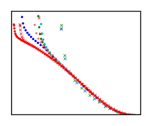
Figure 6(a) presents the experimental data for Reynolds shear stress as $R_{uv}/U^2_e$ versus $y/\delta _e$. Given the scatter in the experimental data, it is challenging to determine precisely the maximum Reynolds shear stress location and value. For instance, figure 6(a) shows that the maximum $R_{uv}$ occurs at a wall-normal location $y/\delta _e \approx 0.6$ for the data of Maciel et al. (Reference Maciel, Rossignol and Lemay2006) at $x=1.615$, but this may not be the actual peak location. The new outer scaling for the Reynolds shear stress is presented in figure 6(b); the scatter is related to the uncertainties in estimating the maximum Reynolds shear stress locations and values from experimental measurements.

Figure 6. Experimental data for Reynolds shear stress. (a) Plots of $R_{uv}/U^2_e$ versus $y/\delta _e$. (b) New outer scaling for Reynolds shear stress.

Reynolds shear stress data from numerical simulation are presented in figure 7. At the beginning of the simulation domain of LES(m13) and LES(m18) ($\times$ symbols in the figure), the maximum Reynolds shear stress occurs closer to the wall, indicating that the flow at those stations is more similar to the ZPG TBL. When the APG effect is sufficient, the maximum Reynolds shear stress locations shift outwards, as shown in figure 6(a). Using the new outer scaling, the simulation data display better collapse, as shown in figure 7(b). An approximation function for the normalized Reynolds shear stress is found by curve fitting as

(3.3)\begin{equation} \frac{R_{uv}}{R_{uv}|_{max}} \approx \exp(-(1.3 y^*)^2 - 0.385 (1.3 y^*)^4). \end{equation}

Figure 7. Numerical simulation data for Reynolds shear stress. (a) Plots of $R_{uv}/U^2_e$ versus $y/\delta _e$. (b) New outer scaling for Reynolds shear stress. Data: LES from Bobke et al. (Reference Bobke, Vinuesa, Örlü and Schlatter2017), DNS from Kitsios et al. (Reference Kitsios, Sekimoto, Atkinson, Sillero, Borrell, Gungor, Jiménez and Soria2017).

The similarities and differences between the approximate equations of $U^*$, $V^*$ and $R^*_{uv}$ for the outer region of the APG TBL and planar turbulent mixing layers are summarized in table 5. In planar turbulent mixing layers, the self-similar transverse location is typically denoted as $\xi = (y-y_{05})/\delta$, where $y_{05}$ is the transverse location at which the mean axial velocity is the average of the high-speed stream $U_h$ and low-speed stream $U_l$. The parameter $1.81\xi$ in the planar turbulent mixing layer equations arises from the definition of the mixing layer half-width using the error function (see Pope Reference Pope2000 or Wei et al. Reference Wei, Li and Livescu2022a). In the approximate $U^*$ equations, the difference between $1.3 y^*$ in the APG TBL and $1.81 \xi$ in the planar turbulent mixing layer comes from the different definitions of flow width. To better fit the data near the boundary layer edge, an additional term $0.21 (1.3 y^*)^4$ is introduced in the APG TBL equation. In the approximate $V^*$ equations, the differences between the APG TBL and mixing layers come from the differences in the boundary conditions and the reference velocity scale $V_{ref}$. In the approximate $R^*_{uv}$ equation for APG TBL, the term $-0.385 (1.3 y^*)^4$ is also introduced, to better fit the data near the boundary layer edge.

Table 5. Approximate functions for the outer region of the APG TBL and planar turbulent mixing layer. In the planar turbulent mixing layer equations, $U_h$ is the high speed, $U_l$ is the low speed, $U_{avg}=0.5(U_h+U_l)$ is the average speed of the two streams, and $o'$ is the location where the mean axial velocity is $U_{avg}$. The coefficients in the planar turbulent mixing equations are based on $a=0.5518$ and $B=-0.25$ in Wei et al. (Reference Wei, Li and Livescu2022a).

4. Approximate reference scales for the outer region of the APG TBL

In § 2, the new outer scales are determined based on the maximum Reynolds shear stress location $y_{m}$. However, the values of $y_{m}$, $U_{m}$, $V_{m}$ and $R_{uv}|_{max}$ are not known a priori, so it is desirable to obtain approximate scales based on parameters that are easier to obtain. Figure 8 presents the ratio of $(\delta _e -y_{m})/\delta _e$ versus $x/\delta _0$ from experimental data and numerical simulation data, including both flows in or approaching equilibrium (Skåre & Krogstad Reference Skåre and Krogstad1994; Bobke et al. Reference Bobke, Vinuesa, Örlü and Schlatter2017) and streamwise evolving flows (Marušić & Perry Reference Marušić and Perry1995). Recall that a certain distance is required, in physical experiments or numerical simulations, for the APG to affect the development of the boundary layer. Near the beginning of the boundary layer, the maximum Reynolds shear stress $y_{m}$ is much smaller than $\delta _e$, and the ratio is clearly larger (close to 1 at high Reynolds number flows), as shown in figure 8. Moving downstream, the ratio $(\delta _e-y_{m})/\delta _e$ is found to approach a constant value around $0.6$ for the flows considered here. In other words, at a sufficient distance from the imposition of an APG for flows in or approaching equilibrium, the outer length scale can be approximated as $y_{ref} = \delta _e$.

Figure 8. Ratio of $(\delta _e -y_{m})$ and $\delta _e$. (a) Experimental data. Note that $\delta _{x=x_1}$ is the boundary layer thickness at the first measuring station, not the leading edge. (b) The LES data of Bobke et al. (Reference Bobke, Vinuesa, Örlü and Schlatter2017), and DNS data (mild APG case) of Kitsios et al. (Reference Kitsios, Sekimoto, Atkinson, Sillero, Borrell, Gungor, Jiménez and Soria2017). Here, $\delta _0$ is the boundary layer thickness at the first $x$-grid of numerical simulation.

At this point, it is important to point out that $y_m\sim 0.4\delta _e$ is used only as an approximation to evaluate the new scaling. It is well known that the location of $y_m$ depends on the strength of the pressure gradient (i.e. on $\beta _{RC}$), and for non-equilibrium flows, also on the extent of the velocity defect, on flow history, and on the Reynolds number. An empirical relation for $y_{m}$ might be inferred from (8) in Perry, Marusic & Li (Reference Perry, Marusic and Li1994). To give two examples for streamwise evolving flows, for illustration, a value of $y_m/\delta _e$ at approximately $0.25\unicode{x2013}0.35$ is found for the last stations of the flow of Marusic and Perry, and a value of approximately $0.2$ was found for the flow of Cuvier et al. (Reference Cuvier2017) with an upstream change from a mild favourable pressure gradient (FPG) into an APG. Moreover, it is worth emphasizing that APG TBLs are not generally approaching equilibrium unless they were specifically designed to do so. To conclude, despite these important details, it appears from figure 8 that at a sufficient distance from the imposition of the APG, the outer length scale can be approximated as $y_{ref}=\delta _e$, at least for flows without significant disequilibrating effects due to the imposed streamwise pressure gradient. The estimation $y_m\sim 0.4\delta _e$ can be seen as a low-order approximation, and a higher-order correction could be obtained using, for example, Perry et al. (Reference Perry, Marusic and Li1994).

Figure 2(a) indicates that an approximate reference scale for the mean wall-normal velocity deficit in the outer region of the APG TBL can be developed as

(4.1)\begin{equation} V_{ref} \sim (\delta_e - y_{m})\,\frac{{\rm d}U_e}{{\rm d} x} \sim \delta_e\, \frac{{\rm d}U_e}{{\rm d} x}. \end{equation}

Figure 2(b) indicates that an approximate scale for the mean streamwise velocity deficit in the outer region of APG TBL can be developed as

(4.2)\begin{equation} U_{ref} \sim U_e. \end{equation}

Figure 2(d) indicates that an approximate reference scale for the Reynolds shear stress in the outer region of the APG TBL can be developed as

(4.3)\begin{equation} R_{uv,{ref}} \sim U_e (\delta_e - y_{m})\,\frac{{\rm d}U_e}{{\rm d} x} \sim \delta_e U_e\,\frac{{\rm d}U_e}{{\rm d} x}. \end{equation}

Note that the approximate scale for the Reynolds shear stress is a mixed scale of $U_e V_{ref}$, and scales with the local streamwise pressure gradient. The approximate reference scales are valid only at a sufficient distance from imposition of the APG (assuming no continuously disequilibrating effects due to the streamwise pressure gradient distribution). For comparison, the reference scales and their approximations for the outer region of the APG TBL are listed in table 6.

Table 6. Reference scales in the outer region of the APG TBL.

5. Relation to results of previous analysis

As reviewed in the Introduction, a number of scales have been proposed previously to describe the flow in the outer region of an APG TBL. Here, we show that the new scales proposed in this work are closely related to several proposed previously, particularly the Zagarola–Smits scales, the scales based on the inflection point of the mean streamwise velocity profile, and the scales of Castillo & George (Reference Castillo and George2001).

5.1. Relation with Zagarola–Smits velocity scale

The Zagarola–Smits velocity scale $U_{zs}$ has been used widely in the scaling of the mean streamwise velocity deficit in both ZPG and APG TBLs. Here, we show that the outer velocity scale $U_e - U_{m}$ proposed in the present paper is closely related to $U_{zs}$. The mass displacement thickness used in the definition of $U_{zs}$ is typically defined by integration from the wall to infinity (see e.g. Schlichting Reference Schlichting1979), but it can also be approximated as

(5.1)\begin{equation} \delta^* \equiv \int_0^\infty \frac{U_e - U}{U_e}\,{{\rm d} y} \approx \int_0^{\delta_e} \frac{U_e - U}{U_e}\,{{\rm d} y}. \end{equation}

Then the Zagarola–Smits scale (Zagarola & Smits Reference Zagarola and Smits1998a,Reference Zagarola and Smitsb) can be written as

(5.2)\begin{equation} U_{ZS} = U_e\,\frac{\delta^*}{\delta_e} = (U_e - U_m)\,\frac{\delta_e - y_{m}}{\delta_e} \int_{(0-y_{m})/(\delta_e - y_{m})}^1 \left(\frac{U_e -U}{U_e - U_{m}} \right) {\rm d}\!\left(\frac{y-y_{m}}{\delta_e - y_{m}}\right). \end{equation}

As shown in figure 8, the ratio $(\delta _e - y_{m})/\delta _e$ approaches a constant around $0.6$ in the APG TBL. Figures 3 and 4 show that $(U_e-U)/(U_e-U_{m})$ profiles collapse well in the outer region. For moderate APG TBLs, figures 3(b) and 4(b) show that the profile of $(U_e-U)/(U_e-U_{m})$ rises sharply in the near-wall region. In other words, the deviation of $(U_e-U)/(U_e-U_{m})$ from the approximate (3.1) is significant only in the near-wall region, which occupies a very small fraction of $(y-y_{m})/(\delta _e-y_{m})$ in figures 3(b) and 4(b). At a strong APG TBL ($x=1.615$ m in the study of Maciel et al. Reference Maciel, Rossignol and Lemay2006), the near-wall profile of $(U_e-U)/(U_e-U_{m})$ deviates only slightly from the curve valid for the outer layer. Therefore, the integral in (5.2) over the entire boundary layer can be obtained approximately from (3.1). The new outer scale proposed in the present work is then closely related to the Zagarola–Smits scale, $U_e - U_{m} \sim U_{ZS}$.

The Zagarola–Smits velocity scale and the new outer velocity scale $U_e - U_{m}$ were calculated from the experimental and LES data, and the ratio $U_{zs}/(U_e - U_{m})$ is presented in figure 9. The scatter, especially in the experimental data, is likely caused by the uncertainty in the determination of the maximum Reynolds shear stress location $y_m$. The experimental and simulation data indicate that $U_{zs}/(U_e - U_{m}) \approx 0.8$ at a sufficient distance from the imposition of APG, which supports the conclusion that the new outer velocity scale is indeed closely related to $U_{zs}$.

Figure 9. Ratio of Zagarola–Smits velocity scale and the new outer velocity scale $(U_e - U_{m})$. (a) Experimental data. (b) The LES data of Bobke et al. (Reference Bobke, Vinuesa, Örlü and Schlatter2017), and DNS data (mild APG case) of Kitsios et al. (Reference Kitsios, Sekimoto, Atkinson, Sillero, Borrell, Gungor, Jiménez and Soria2017).

5.2. Mean streamwise velocity inflection point and maximum Reynolds shear stress location

In several previous studies of APG TBL (see e.g. Schatzman & Thomas Reference Schatzman and Thomas2017; Maciel et al. Reference Maciel, Wei, Gungor and Simens2018), the inflection point $y_{IP}$ of the mean streamwise velocity has been used to define outer scales. Typically, the mean streamwise velocity at $y_{IP}$ is used directly as an outer velocity scale. Our scaling patch analysis also allows use of the inflection point to define the outer length scale as $\delta _e - y_{IP}$, the outer velocity scale for the mean streamwise velocity deficit as $U_e - U_{IP}$, the outer velocity scale for the mean wall-normal velocity deficit as $V_e - V_{IP}$, and the scale for the Reynolds shear stress as $Re_{uv}(y_{IP})$.

The use of $y_m$ in the present work can be viewed as a generalization of the idea of Schatzman & Thomas (Reference Schatzman and Thomas2017), since the maximum of the Reynolds shear stress $y_m$ is located near the inflection point of the mean velocity profile in the outer part of TBLs. However, the mean velocity inflection point in the outer layer occurs only under strong pressure gradients, whereas the outer maximum of the Reynolds shear stress appears already in a mild or moderate APG. Moreover, $y_{m}$ is significantly easier to determine from experimental or simulation data. As an example, figure 10(a) shows the mean velocity gradient profiles at the first and last stations in the simulation of Bobke et al. (Reference Bobke, Vinuesa, Örlü and Schlatter2017). The inset shows a monotonic decrease of ${\rm d}U/{{\rm d} y}$ with $y$ at the first station. At the last station, ${\rm d}U/{{\rm d} y}$ first decreases from the wall to a smaller value, then rises to a peak (the inflection point), and decreases again towards the boundary layer edge. In practice, it is challenging to obtain an accurate and smooth profile of ${\rm d}U/{{\rm d} y}$, even from numerical simulation data. Hence the determination of the inflection point may lead to significant uncertainties. Figure 10(b) presents the Reynolds shear stress profiles for the two locations used in figure 10(a). The maximum Reynolds shear stress location $y_{m}$ can be determined more easily from the simulation data. For accurate determination of $y_{m}$ in experimental measurements, sufficient spatial resolution and smoothness of the data are required.

Figure 10. (a) Typical shapes of ${\rm d}U/{{\rm d} y}$ in the APG TBL. (b) Typical shapes of Reynolds shear stress in the APG TBL.

An additional, even more important, advantage of using the maximum shear stress location to define the outer layer scaling for the APG TBL is the direct connection to free shear turbulent flows. In this sense, the outer part of a TBL resembles a free shear flow; the comparison echoes the wake flow analogy of Coles & Hirst (Reference Coles and Hirst1969) and the mixing layer analogy of Maciel et al. (Reference Maciel, Wei, Gungor and Simens2018).

5.3. Relation to results of Castillo and George

Castillo & George (Reference Castillo and George2001) performed a similarity analysis of the outer part of an APG TBL. The boundary layer thickness $\delta _e$ was used as the reference scale for the outer flow. They derived a dimensionless mean momentum equation using two self-similar functions of $f_{op\infty }=(U-U_e)/U_{ref}$, $r_{op\infty } = -\langle uv\rangle /R_{uv,{ref}}$ and their derivatives $f'_{op\infty }$ and $r'_{op\infty }$. (In their work, Castillo & George (Reference Castillo and George2001) denoted the outer velocity scale as $U_{so}$ and the Reynolds shear stress scale as $R_{so}$.) For the dimensionless equation to yield equilibrium similarity solutions, Castillo & George (Reference Castillo and George2001) argued that all the pre-factors of the terms in their dimensionless equation should have the same $x$ dependence, and must remain proportional to each other as the flow develops. Consequently, they proposed the outer scales for the APG TBL as

(5.3)\begin{gather} U_{ref} \sim U_e, \end{gather}
(5.4)\begin{gather}R_{uv,{ref}} \sim U^2_{ref}\,\frac{{\rm d}\delta}{{\rm d} x}. \end{gather}

Therefore, the outer velocity scale used by Castillo & George (Reference Castillo and George2001) is the same as the approximation (4.2). Castillo & George (Reference Castillo and George2001) specified additional independent constraints

(5.5)\begin{equation} \frac{{\rm d}\delta}{{\rm d} x} \sim \frac{\delta}{U_e}\,\frac{{\rm d}U_e}{{\rm d} x} \sim \frac{\delta}{\rho U^2_e}\,\frac{{\rm d}P_e}{{\rm d}x}. \end{equation}

Applying the relation in (5.5), the reference scale of Castillo & George (Reference Castillo and George2001) for the Reynolds shear stress can be written as $R_{uv,{ref}} \sim \delta U_e \, {\rm d}U_e/{{\rm d} x}$, which is similar to the approximation (4.3) developed in the present work.

In the present work, the self-similarity assumption is not applied directly in the scaling patch analysis of the mean momentum equation (see § 2), and the $x$ derivative is not involved except in ${\rm d}U_e/{{\rm d}x}$. The constraint equation (5.5) suggested by Castillo & George (Reference Castillo and George2001) can be obtained by a scaling patch analysis of the mean continuity equation, supplemented by a self-similarity assumption as in the analysis of planar turbulent wake flows (Wei et al. Reference Wei, Livescu and Liu2022b).

Substituting the normalized variables, the mean continuity equation (2.1a) becomes

(5.6)\begin{equation} 0 = \frac{\partial (U_e - U_{ref}U^*)}{\partial x} + \frac{\partial (V_e-V_{ref}V^*)}{\partial y}, \end{equation}

which can be rearranged as

(5.7)\begin{equation} 0 = \frac{{\rm d}U_e}{{\rm d} x} - \frac{{\rm d}U_{ref}}{{\rm d} x}\,U^* - U_{ref}\,\frac{\partial U^*}{\partial x} - \frac{V_{ref}}{y_{ref}}\,\frac{\partial V^*}{\partial y^*}. \end{equation}

Note that $V_e$ is a function of $x$ only, not depending on $y$. Multiplying $y_{ref}/V_{ref}$ onto (5.7) yields a dimensionless equation

(5.8)\begin{equation} 0 = \frac{y_{ref}\,\dfrac{{\rm d}U_e}{{\rm d} x}}{V_{ref}} - \dfrac{y_{ref}\,\dfrac{{\rm d}U_{ref}}{{\rm d} x}}{V_{ref}} U^* - \dfrac{y_{ref}\, U_{ref} }{V_{ref}}\,\dfrac{\partial U^*}{\partial x} - \dfrac{\partial V^*}{\partial y^*}. \end{equation}

The self-similarity assumption is introduced now to transform the derivative $\partial U^*/\partial x$ as

(5.9)\begin{align} \frac{\partial U^*}{\partial x} & = \frac{{\rm d} U^*}{{{\rm d} y}^*}\,\frac{\partial y^*}{\partial x} = \frac{{\rm d} U^*}{{{\rm d} y}^* }\,\frac{\partial (y-y_{m})/y_{ref}}{\partial x} \nonumber\\ & ={-} \frac{1}{y_{ref}}\,\frac{{\rm d}y_{m}}{{\rm d} x}\,\frac{{\rm d} U^*}{{{\rm d} y}^*} - \frac{1}{y_{ref}}\,\frac{{\rm d}y_{ref}}{{\rm d} x}\,y^*\,\frac{{\rm d}U^*}{{{\rm d} y}^*}. \end{align}

Then (5.8) becomes

(5.10)\begin{equation} 0 = \frac{y_{ref}\,\dfrac{{\rm d}U_e}{{\rm d} x}}{V_{ref}} - \dfrac{y_{ref}\,\dfrac{{\rm d}U_{ref}}{{\rm d} x}}{V_{ref}}\,U^* + \dfrac{U_{ref}}{V_{ref}}\,\dfrac{{\rm d}y_{m}}{{\rm d} x}\,\dfrac{{\rm d} U^*}{{{\rm d} y}^*} + \dfrac{U_{ref}}{V_{ref}}\,\dfrac{ {\rm d}y_{ref}}{{\rm d} x}\,y^*\,\dfrac{{\rm d}U^*}{{{\rm d} y}^*} - \dfrac{{\rm d}V^*}{{{\rm d} y}^*}. \end{equation}

Note that $y^*$, $U^*$ and $V^*$ in (5.10) are of order $O(1)$. Moreover, $\partial U^*/\partial y^*$ and $\partial V^*/\partial y^*$ are also of order $O(1)$ in the outer region of the APG TBL, as $U^*$ and $V^*$ are smooth functions of $y^*$. The first term in (5.10) is about $0.5$ (see figure 2a), so it has a nominal order 1. The pre-factor to the second term also has a nominal order 1. Therefore, the pre-factor of the third and fourth terms in (5.10) must be

(5.11a,b)\begin{equation} \frac{U_{ref}}{V_{ref}}\,\frac{{\rm d}y_{m}}{{\rm d} x} \leqslant O(1), \quad \frac{U_{ref}}{V_{ref}}\,\frac{{\rm d}y_{ref}}{{\rm d}x} \leqslant O(1). \end{equation}

The constraint equation (5.5) suggested by Castillo & George (Reference Castillo and George2001) can be obtained by setting the pre-factors of the first and fourth terms in (5.10) proportional to each other:

(5.12)\begin{equation} y_{ref}\,\frac{{\rm d}U_e}{{\rm d} x} \sim U_{ref}\,\frac{{\rm d}y_{ref}}{{\rm d}x}. \end{equation}

Therefore, the self-similarity analysis of Castillo & George (Reference Castillo and George2001) can also be developed from a scaling patch analysis of the mean continuity equation.

6. Summary

The scaling patch approach is applied in the present work to develop a new scaling of the mean momentum equation for the outer region of the APG TBL. The flow properties at the maximum Reynolds shear stress location $y_{m}$ are found to play a key role in the new outer scaling. A new outer length scale is proposed as $\delta _e - y_{m}$, a new velocity for the mean streamwise velocity deficit is proposed as $U_e - U_{m}$, and a new velocity for the mean transverse velocity deficit is proposed as $V_e - V_{m}$. The new scales are verified against experimental and numerical APG TBL data over a wide range of Reynolds numbers and strengths of pressure gradient. Approximate scales are also developed for the convenience of practical application, and the relation between the new scales and previous analysis has been clarified. In figures 3(b), 4(b), 6(b) and 7(b), the new outer scaling is applied to experimental and numerical data at the first and last $x$-locations. These figures show minor differences in the scaled profiles between the first and last station. Figure 11 shows that, not surprisingly, the new outer scaling works better when only the rear half of the simulation data are presented.

Figure 11. New outer scaled profiles in the rear half of the simulation domain. (a) Mean streamwise velocity deficit. (b) Reynolds shear stress.

In previous investigations of the APG TBL, the mean transverse velocity $V$ was rarely studied. In the present work, we demonstrate that the characteristics of $V$ are important in the understanding and scaling of the mean flow in the outer region of the APG TBL. In fact, the proper scale for the Reynolds shear stress is a mixed scale of $U_e$ and $V_{ref}$ (see (4.1) and (4.3)).

The new outer scaling arises directly from a scaling patch analysis of the mean momentum equation. Two distinct differences between the new outer scaling and previous studies are the outer length scale and the outer scale for the mean transverse velocity deficit. The new outer scaling for APG TBL is cast in a form that is similar to that for planar turbulent wake flows or planar turbulent mixing layers. Therefore, the new outer scaling developed here opens a pathway for future investigation on the similarities and differences between the outer region of the APG TBL and free shear turbulent flows, such as turbulent wakes or turbulent mixing layers.

Funding

We are grateful to Dr Bobke, Dr Kitsios, Dr Skåre, and their groups for sharing the simulation and experimental data. The funding of the project ‘Complex Wake Flows’ by DFG (grant no. KN 888/3-2) of the second author T.K. is gratefully acknowledged.

Declaration of interests

The authors report no conflict of interest.

References

REFERENCES

Afzal, N. 1982 Fully developed turbulent flow in a pipe: an intermediate layer. Arch. Appl. Mech. 52 (6), 355377.Google Scholar
Bobke, A., Vinuesa, R., Örlü, R. & Schlatter, P. 2017 History effects and near equilibrium in adverse-pressure-gradient turbulent boundary layers. J. Fluid Mech. 820, 667692.CrossRefGoogle Scholar
Castillo, L. & George, W.K. 2001 Similarity analysis for turbulent boundary layer with pressure gradient: outer flow. AIAA J. 39 (1), 4147.CrossRefGoogle Scholar
Clauser, F.H. 1954 Turbulent boundary layers in adverse pressure gradients. J. Aeronaut. Sci. 21, 91108.CrossRefGoogle Scholar
Coles, D.E. & Hirst, E.A. 1969 Computation of Turbulent Boundary Layers – 1968 AFOSR-IFP-Stanford Conference. Thermosciences Division, Department of Mechanical Engineering, Stanford University.Google Scholar
Corrsin, S. 1943 Investigation of flow in an axially symmetric heated jet of air. NACA Tech. Rep. WR W-94. California Institute of Technology.Google Scholar
Corrsin, S. & Kistler, A.L. 1955 Free-stream boundaries of turbulent flows. NACA Tech. Rep. 1244. California Institute of Technology.Google Scholar
Cuvier, C., et al. 2017 Extensive characterisation of a high Reynolds number decelerating boundary layer using advanced optical metrology. J. Turbul. 18, 929972.CrossRefGoogle Scholar
Eisfeld, B. 2021 Characteristics of incompressible free shear flows and implications for turbulence modeling. AIAA J. 59 (1), 180195.Google Scholar
Elsberry, K., Loeffler, J., Zhou, M.D. & Wygnanski, I. 2000 An experimental study of a boundary layer that is maintained on the verge of separation. J. Fluid Mech. 423, 227261.CrossRefGoogle Scholar
Fife, P. 2006 Scaling approaches to steady wall-induced turbulence. arXiv:2301.08740.Google Scholar
Fife, P., Klewicki, J., McMurtry, P. & Wei, T. 2005 Multiscaling in the presence of indeterminacy: wall-induced turbulence. Multiscale Model. Simul. 4 (3), 936959.CrossRefGoogle Scholar
Fife, P., Klewicki, J. & Wei, T. 2009 Time averaging in turbulence settings may reveal an infinite hierarchy of length scales. Discret. Contin. Dyn. A 24 (3), 781.CrossRefGoogle Scholar
George, W.K., Stanislas, M. & Laval, J.P. 2012 New insights into adverse pressure gradient boundary layers. In Progress in Turbulence and Wind Energy IV (ed. M. Oberlack, J. Penke, A. Talamelli, L. Castillo & M. Hölling), Springer Proceedings in Physics, vol. 141. Springer.CrossRefGoogle Scholar
Görtler, H. 1942 Berechnung von Aufgaben der freien Turbulenz auf Grund eines neuen Näherungsansatzes. Z. Angew. Math. Mech. 22 (5), 244254.CrossRefGoogle Scholar
Gungor, A.G., Maciel, Y., Simens, M.P. & Soria, J. 2016 Scaling and statistics of large-defect adverse pressure gradient turbulent boundary layers. Intl J. Heat Fluid Flow 59, 109124.CrossRefGoogle Scholar
von Kármán, T. 1930 Mechanische Ähnlichkeit und Turbulenz. In Proceedings of the 3rd International Congress on Applied Mechanics, Stockholm, Sweden, pp. 85–93. Weidmannsche Buchh.Google Scholar
Kitsios, V., Atkinson, C., Sillero, J.A., Borell, G., Gungor, A.G., Jimenez, J. & Soria, J. 2016 Direct numerical simulation of a self-similar adverse pressure gradient turbulent boundary layer. Intl J. Heat Fluid Flow 61, 129136.Google Scholar
Kitsios, V., Sekimoto, A., Atkinson, C., Sillero, J.A., Borrell, G., Gungor, A.G., Jiménez, J. & Soria, J. 2017 Direct numerical simulation of a self-similar adverse pressure gradient turbulent boundary layer at the verge of separation. J. Fluid Mech. 829, 392419.Google Scholar
Klebanoff, P. 1955 Characteristics of turbulence in a boundary layer with zero pressure gradient. NACA Tech. Rep. 1247. National Bureau of Standards.Google Scholar
Krug, D., Philip, J. & Marusic, I. 2017 Revisiting the law of the wake in wall turbulence. J. Fluid Mech. 811, 421435.CrossRefGoogle Scholar
Liu, X., Thomas, F.O. & Nelson, R.C. 2002 An experimental investigation of the planar turbulent wake in constant pressure gradient. Phys. Fluids 14 (8), 28172838.CrossRefGoogle Scholar
Long, R.R. & Chen, T.-C. 1981 Experimental evidence for the existence of the ‘mesolayer’ in turbulent systems. J. Fluid Mech. 105, 1959.Google Scholar
Maciel, Y., Rossignol, K.-S. & Lemay, J. 2006 A study of a turbulent boundary layer in stalled-airfoil-type flow conditions. Exp. Fluids 41 (4), 573590.Google Scholar
Maciel, Y., Wei, T., Gungor, A.G. & Simens, M.P. 2018 Outer scales and parameters of adverse-pressure-gradient turbulent boundary layers. J. Fluid Mech. 844, 535.CrossRefGoogle Scholar
Marušić, I. & Perry, A.E. 1995 A wall-wake model for the turbulence structure of boundary layers. Part 2. Further experimental support. J. Fluid Mech. 298, 389407.CrossRefGoogle Scholar
Mehdi, F., Klewicki, J.C. & White, C.M. 2010 Mean momentum balance analysis of rough-wall turbulent boundary layers. Physica D 239 (14), 13291337.CrossRefGoogle Scholar
Mellor, G.L. & Gibson, D.M. 1966 Equilibrium turbulent boundary layers. J. Fluid Mech. 24 (2), 225253.CrossRefGoogle Scholar
Millikan, C.B. 1938 A critical discussion of turbulent flows in channels and circular tubes. In Proceedings of the 5th International Congress for Applied Mechanics (ed. J.P. Den Hartog & H. Peters), pp. 386–392. Wiley.Google Scholar
Monkewitz, P.A., Chauhan, K.A. & Nagib, H.M. 2007 Comparison of mean flow similarity laws in zero pressure gradient turbulent boundary layers. Phys. Fluids 20, 105102.CrossRefGoogle Scholar
Nagano, Y., Tagawa, M. & Tsuji, T. 1993 Effects of adverse pressure gradients on mean flows and turbulence statistics in a boundary layer. In Turbulent Shear Flows (ed. F. Durst, R. Friedrich, B.E. Launder, F.W. Schmidt, U. Schumann & J.H. Whitelaw), vol. 8, pp. 7–21. Springer.Google Scholar
Nickels, T.B. 2004 Inner scaling for wall-bounded flows subject to large pressure gradients. J. Fluid Mech. 521, 217239.CrossRefGoogle Scholar
Perry, A.E., Marusic, I. & Li, J.D. 1994 Wall turbulence closure based on classical similarity laws and the attached eddy hypothesis. Phys. Fluids 6, 10241035.CrossRefGoogle Scholar
Perry, A.E. & Schofield, W.H. 1973 Mean velocity and shear stress distributions in turbulent boundary layers. Phys. Fluids 16, 20682074.CrossRefGoogle Scholar
Pope, S.B. 2000 Turbulent Flows. Cambridge University Press.Google Scholar
Romero, S.K., Zimmerman, S.J., Philip, J. & Klewicki, J.C. 2021 Stress equation based scaling framework for adverse pressure gradient turbulent boundary layers. Intl J. Heat Fluid Flow 93, 108885.CrossRefGoogle Scholar
Rotta, J. 1950 Über die Theorie turbulenter Grenzschichten. Tech. Rep. Mitteilungen aus dem Max-Planck-Institut für Strömungsforschung Nr. 1. (Translated as: On the theory of turbulent boundary layers. NACA Technical Memorandum No. 1344, 1953.).Google Scholar
Schatzman, D.M. & Thomas, F.O. 2017 An experimental investigation of an unsteady adverse pressure gradient turbulent boundary layer: embedded shear layer scaling. J. Fluid Mech. 815, 592642.CrossRefGoogle Scholar
Schlichting, H. 1979 Boundary-Layer Theory. McGraw-Hill, Inc.Google Scholar
Schofield, W.H. 1981 Equilibrium boundary layers in moderate to strong adverse pressure gradient. J. Fluid Mech. 113, 91122.CrossRefGoogle Scholar
Schofield, W.H. & Perry, A.E. 1972 The turbulent boundary layer as a wall confined wake. Tech. Rep. 134. Australian Department of Supply.Google Scholar
Sekimoto, A., Kitsios, V., Atkinson, C., Sillero, J.A., Borell, G., Gungor, A.G., Jimenez, J. & Soria, J. 2019 Outer scaling of self-similar adverse-pressure-gradient turbulent boundary layers. arXiv:1912.05143.Google Scholar
Skåre, P.E. & Krogstad, P.A. 1994 A turbulent equilibrium boundary layer near separation. J. Fluid Mech. 272, 319348.CrossRefGoogle Scholar
Slotnick, J.P. & Heller, G. 2019 Emerging opportunities for predictive CFD for off-design commercial airplane flight characteristics. In 54th 3AF International Conference on Applied Aerodynamics, Paris, pp. 25–27.Google Scholar
Sreenivasan, K.R. & Sahay, A. 1997 The persistence of viscous effects in the overlap region, and the mean velocity in turbulent pipe and channel flows. arXiv:physics/9708016.Google Scholar
Tennekes, H. & Lumley, J.L. 1972 A First Course in Turbulence. MIT Press.CrossRefGoogle Scholar
Townsend, A.A. 1956 The Structure of Turbulent Shear Flow. Cambridge University Press.Google Scholar
Wei, T. 2019 Multiscaling analysis of buoyancy-driven turbulence in a differentially heated vertical channel. Phys. Rev. Fluids 4, 073502.Google Scholar
Wei, T. 2020 Analyses of buoyancy-driven convection. Adv. Heat Transfer 52, 193.CrossRefGoogle Scholar
Wei, T., Fife, P., Klewicki, J. & McMurtry, P. 2005 Properties of the mean momentum balance in turbulent boundary layer, pipe and channel flows. J. Fluid Mech. 522, 303327.Google Scholar
Wei, T., Li, Z. & Livescu, D. 2022 a Scaling patch analysis of planar turbulent mixing layers. Phys. Fluids 34, 115120.CrossRefGoogle Scholar
Wei, T. & Livescu, D. 2021 a Scaling of the mean transverse flow and Reynolds shear stress in turbulent plane jet. Phys. Fluids 33 (3), 035142.CrossRefGoogle Scholar
Wei, T. & Livescu, D. 2021 b Scaling patch analysis of turbulent planar plume. Phys. Fluids 33 (5), 055101.CrossRefGoogle Scholar
Wei, T., Livescu, D. & Liu, X. 2022 b Scaling patch analysis of planar turbulent wake. Phys. Fluids 34, 065116.Google Scholar
Zagarola, M.V. & Smits, A.J. 1998 a Mean-flow scaling of turbulent pipe flow. J. Fluid Mech. 373, 3379.CrossRefGoogle Scholar
Zagarola, M.V. & Smits, A.J. 1998 b A new mean velocity scaling for turbulent boundary layers. ASME Paper No. FEDSM98-4950.Google Scholar
Zhou, A., Pirozzoli, S. & Klewicki, J. 2017 Mean equation based scaling analysis of fully-developed turbulent channel flow with uniform heat generation. Intl J. Heat Mass Transfer 115, 5061.CrossRefGoogle Scholar
Figure 0

Figure 1. Defining the new outer scales for an APG TBL. The data are from experiments of Skåre & Krogstad (1994) at the sixth station (${Re}_\tau \approx 5160$ and $\beta _{RC}=21.2$). The sketch is to illustrate the shapes of the profiles; the magnitudes on the vertical axis do not scale.

Figure 1

Table 1. Conditions at the maximum Reynolds shear stress location $y_{m}$ and boundary layer edge $\delta _e$.

Figure 2

Table 2. Conditions at $y_{m}$ and $\delta _e$.

Figure 3

Figure 2. Parameters in the pre-factors of (2.5). (a) Pre-factor of the first term in (2.5). (b) Plots of $(U_e-U_{m})/U_e$ versus $x$. (c) Plots of $V_e/((\delta _e-y_{m})\,{\rm d}U_e/{{\rm d} x})$ versus $x$. (d) Pre-factor of Reynolds shear stress gradient term in (2.5). The LES data are from Bobke et al. (2017), and the DNS data are from Kitsios et al. (2017). To prevent clutter, only every $80$ $x$-grids are plotted.

Figure 4

Table 3. Values of the pre-factors of terms in (2.5), computed from the LES data of Bobke et al. (2017).

Figure 5

Table 4. Experimental and numerical simulation of APG TBL. To prevent clutter, only the first and last $x$-stations were used from each data set; ix for the LES and DNS data refers to the grid number in the x-direction.

Figure 6

Figure 3. Experimental data of mean streamwise velocity. (a) Plots of $U/U_e$ versus $y/\delta$. (b) New outer scaling for the mean streamwise velocity deficit. Data: NTT from Nagano et al. (1993), SK from Skåre & Krogstad (1994), MP from Marušić & Perry (1995), and MRL from Maciel et al. (2006).

Figure 7

Figure 4. Numerical simulation data of mean streamwise velocity. (a) Plots of $U/U_e$ versus $y/\delta$. (b) New outer scaling for the mean streamwise velocity deficit. Data: LES from Bobke et al. (2017), DNS from Kitsios et al. (2017).

Figure 8

Figure 5. Numerical simulation data of mean wall-normal velocity deficit. (a) Plots of $V/V_e$ versus $y/\delta _e$. (b) New outer scaling for the mean wall-normal velocity deficit. Data: LES from Bobke et al. (2017), DNS from Kitsios et al. (2017).

Figure 9

Figure 6. Experimental data for Reynolds shear stress. (a) Plots of $R_{uv}/U^2_e$ versus $y/\delta _e$. (b) New outer scaling for Reynolds shear stress.

Figure 10

Figure 7. Numerical simulation data for Reynolds shear stress. (a) Plots of $R_{uv}/U^2_e$ versus $y/\delta _e$. (b) New outer scaling for Reynolds shear stress. Data: LES from Bobke et al. (2017), DNS from Kitsios et al. (2017).

Figure 11

Table 5. Approximate functions for the outer region of the APG TBL and planar turbulent mixing layer. In the planar turbulent mixing layer equations, $U_h$ is the high speed, $U_l$ is the low speed, $U_{avg}=0.5(U_h+U_l)$ is the average speed of the two streams, and $o'$ is the location where the mean axial velocity is $U_{avg}$. The coefficients in the planar turbulent mixing equations are based on $a=0.5518$ and $B=-0.25$ in Wei et al. (2022a).

Figure 12

Figure 8. Ratio of $(\delta _e -y_{m})$ and $\delta _e$. (a) Experimental data. Note that $\delta _{x=x_1}$ is the boundary layer thickness at the first measuring station, not the leading edge. (b) The LES data of Bobke et al. (2017), and DNS data (mild APG case) of Kitsios et al. (2017). Here, $\delta _0$ is the boundary layer thickness at the first $x$-grid of numerical simulation.

Figure 13

Table 6. Reference scales in the outer region of the APG TBL.

Figure 14

Figure 9. Ratio of Zagarola–Smits velocity scale and the new outer velocity scale $(U_e - U_{m})$. (a) Experimental data. (b) The LES data of Bobke et al. (2017), and DNS data (mild APG case) of Kitsios et al. (2017).

Figure 15

Figure 10. (a) Typical shapes of ${\rm d}U/{{\rm d} y}$ in the APG TBL. (b) Typical shapes of Reynolds shear stress in the APG TBL.

Figure 16

Figure 11. New outer scaled profiles in the rear half of the simulation domain. (a) Mean streamwise velocity deficit. (b) Reynolds shear stress.