2.1. Preliminaries

We consider the scattering of linear water waves by $N+1$ parallel surface-piercing vertical barriers in a fluid domain of infinite horizontal extent and constant, finite depth $H$. A two-dimensional Cartesian coordinate system $(x,z)$ is used, where the $z$ axis points vertically upwards and the horizontal coordinate $x$ corresponds to the direction of propagation of the waves. The fluid domain is bounded vertically by a flat seabed at $z=-H$ and a free surface located at $z=0$ when at equilibrium.

Each vertical barrier is of infinitesimal thickness and is situated at $x=x^{(n)}$, where $x^{(n)}\in \mathbb {R}$ for all $n\in \{0,\ldots,N\}$, and $x^{(n)}>x^{(n-1)}$ for $n\geq 1$. Each barrier is defined by the set of points $\varGamma _b^{(n)}=\{(x^{(n)},z)|z\geq -d^{(n)}\}$, where $d^{(n)}\in (-H,0)$ is the submergence depth of the $n$th barrier. A schematic of this geometry is given in figure 1.

Figure 1. Schematic of the multiple vertical barrier problem.

We denote by $\varOmega$ the region occupied by the fluid at equilibrium, that is

(2.1)\begin{equation} \varOmega=\left\{(x,z)\in\mathbb{R}\times({-}H,0)\left|(x,z)\notin\bigcup_{n=0}^{N}\varGamma_b^{(n)} \right.\right\}. \end{equation}

We also define the following subregions:

(2.2)\begin{equation} \left.\begin{array}{c} \varOmega^{(0)} = \{(x,z)|x< x^{(0)}\text{ and }z\in({-}H,0)\},\\[3pt] \varOmega^{(n)} = \{(x,z)|x\in({-}x^{(n-1)},x^{(n)})\text{ and } z\in({-}H,0)\}\quad \text{for all }n\in\{1,\ldots,N\},\\[3pt] \varOmega^{(N+1)} = \{(x,z)|x>x^{(N)}\text{ and }z\in({-}H,0)\}. \end{array}\right\} \end{equation}

In order to apply linear water wave theory to this problem, we assume that the steepness of the free-surface elevation of the incident waves is small. Thus, we consider the fluid to be inviscid, incompressible and undergoing irrotational, time-harmonic motion with angular frequency $\omega$. We assume that there is no normal flow across the seabed and the barriers. The velocity field of the fluid can therefore be expressed as the spatial gradient of some potential $\varPhi :\varOmega \times \mathbb {R}\to \mathbb {R}$, which is of the form

(2.3)\begin{equation} \varPhi(x,z,t) = {{\rm Re}}(\phi(x,z)\exp(-\mathrm{i}\omega t)). \end{equation}

The complex-valued spatial function $\phi$ then satisfies the following boundary value problem:

(2.4a)$$\begin{gather} \Delta\phi=0 \quad \forall\, (x,z)\in \varOmega, \end{gather}$$

(2.4b)$$\begin{gather}\partial_z\phi=0 \quad \text{for }z={-}H, \end{gather}$$

(2.4c)$$\begin{gather}\partial_z\phi=\frac{\omega^{2}}{g}\phi \quad \text{for } z=0, \end{gather}$$

(2.4d)$$\begin{gather}\partial_x\phi= 0 \quad \text{for all }(x,z)\in\bigcup_{n=0}^{N} \varGamma_b^{(n)}, \end{gather}$$

where (2.4c) is the linear free-surface condition with $g$ denoting acceleration due to gravity.

Since $\phi$ is twice differentiable, it must be continuous and have a continuous first partial derivative with respect to $x$ across the gaps beneath each barrier. This can be expressed in terms of one-sided limits as

(2.5a,b)\begin{equation} \lim_{x\to x^{(n)-}}\phi(x,z)=\lim_{x\to x^{(n)+}}\phi(x,z) \quad\mbox{and}\quad \lim_{x\to x^{(n)-}}\partial_x\phi(x,z)=\lim_{x \to x^{(n)+}}\partial_x\phi(x,z), \end{equation}

for all $n=0,\ldots,N$, where $z\in (-H,-d^{(n)})$. We require that $|\phi |$ remains finite as ${x\to \pm \infty }$. The solution must also obey an appropriate Sommerfeld radiation condition, which enforces that the scattered plane waves must propagate away from the array of barriers (see (2.12)).

The submerged edges of the barriers located at $(x^{(n)},-d)$ create singularities of order $-1/2$ in the fluid velocity (Evans & Morris Reference Evans and Morris1972; Mosig Reference Mosig2018). Thus we require that for all $n\in \{0,\ldots,N\}$

(2.6)\begin{equation} ((x-x^{(n)})^{2}+(z+d^{(n)})^{2})^{1/2}\nabla \phi\to \boldsymbol{0}\mbox{ as }((x-x^{(n)})^{2}+(z+d^{(n)})^{2})^{1/2}\to 0. \end{equation}

The general solution to (2.4a)–(2.4c) is obtained using separation of variables:

(2.7)\begin{equation} \phi(x,z) = \left\{\begin{array}{ll} \begin{aligned} & \displaystyle \sum_{m=0}^{\infty} (A_m^{(n)}\exp(\mathrm{i}k_m(x-x^{(n)}))\\ & \quad +B_m^{(n)}\exp(-\mathrm{i}k_m(x-x^{(n)})))\psi_m^{(0)}(z) \end{aligned} & \begin{aligned} & \mbox{for } (x,z)\in\varOmega^{(n)}\\ & \quad \mbox{where }n\in\{0,\ldots,N\},\end{aligned}\\ \begin{aligned} & \displaystyle \sum_{m=0}^{\infty} (A_m^{(N+1)}\exp(\mathrm{i}k_m(x-x^{(N)}))\\ & \quad +B_m^{(N+1)}\exp(-\mathrm{i}k_m(x-x^{(N)})))\psi_m^{(0)}(z) \end{aligned} & \mbox{for } (x,z)\in\varOmega^{(N+1)}. \end{array}\right. \end{equation}

The quantities $k_m$ are the solutions to the free-surface dispersion relation

(2.8)\begin{equation} k\tanh kH=\frac{\omega^{2}}{g}.\end{equation}

We use the convention that ${k_0=2{\rm \pi} /\lambda \in \mathbb {R}_+}$, where $\lambda$ is the wavelength of the propagating waves, and that ${-\mathrm {i}k_n\in ((n-1){\rm \pi} /H,n{\rm \pi} /H)}$ for all ${n\in \mathbb {N}}$. The vertical eigenfunctions are defined as

(2.9)\begin{equation} \psi_m^{(0)}(z)=\beta_m^{{-}1/2}\cosh(k_m(z+H)), \end{equation}

where the superscript $(0)$ has been included for consistency with § 3. The normalisation constants $\beta _m=\sinh (2k_m H)/(4k_m H)+\frac {1}{2}$ are chosen so that the vertical eigenfunctions satisfy

(2.10)\begin{equation} \int_{{-}H}^{0}\psi_m^{(0)}(\xi)\psi_p^{(0)}(\xi)\, {{\rm d}} \xi = H\delta_{m p}, \end{equation}

for all $m,p\in \{0\}\cup \mathbb {N}$, where $\delta _{mp}$ is the Kronecker delta.

The fluid motion is forced by incident plane waves with angular frequency $\omega$. This forcing determines the incident potential on the exterior regions of the fluid, which is of the form

(2.11)\begin{equation} \phi_{{in}}(x,z)= \begin{cases} A_0^{(0)}\exp(\mathrm{i}k_0(x-x^{(0)}))\psi_0^{(0)}(z) & \mbox{for }(x,z)\in\varOmega^{(0)},\\[3pt] B_0^{(N+1)} \exp(-\mathrm{i}k_0(x-x^{(N)}))\psi_0^{(0)}(z) & \mbox{for }(x,z)\in\varOmega^{(N+1)}. \end{cases} \end{equation}

We will mostly consider problems where the forcing originates from the left. In this case, $B_0^{(N+1)}=0$ and the transmission and reflection coefficients are $T=A_0^{(N+1)}/A_0^{(0)}$ and $R=B_0^{(0)}/A_0^{(0)}$, respectively. Since $|\phi |$ remains finite as $x\to \pm \infty$, we must have $A_m^{(0)}=B_m^{(N+1)}=0$ for all $m\geq 1$. The Sommerfeld radiation condition is thus

(2.12)\begin{equation} \phi(x,z)-\phi_{{in}}(x,z)\sim \begin{cases} B_0^{(0)}\exp(-\mathrm{i}k_0(x-x^{(0)}))\psi_0^{(0)}(z) & \mbox{as }x\to-\infty,\\[3pt] A_0^{(N+1)}\exp(\mathrm{i}k_0(x-x^{(N)}))\psi_0^{(0)}(z) & \mbox{as }x\to\infty, \end{cases} \end{equation}

for all $z\in (-H,0)$.

2.2. Overview of the solution technique

We invoke the continuity conditions (2.5a,b) and the no-flow condition (2.4d) for each barrier in order to map the amplitudes of waves incident on the $n$th barrier to the amplitudes of the waves scattered by that barrier. This mapping is approximated by the scattering matrix relation

(2.13)\begin{equation} {\boldsymbol{\mathsf{S}}}^{(n,n+1)}\begin{bmatrix} \boldsymbol{A}^{(n)}\\\boldsymbol{B}^{(n+1)}\end{bmatrix}= \begin{bmatrix} \boldsymbol{A}^{(n+1)}\\\boldsymbol{B}^{(n)}\end{bmatrix} \end{equation}

for $n\in \{0,\ldots,N\}$. Here, $\boldsymbol {A}^{(n)}$ and $\boldsymbol {B}^{(n)}$ are vectors with entries $A_m^{(n)}$ and $B_m^{(n)}$, for $0\leq m \leq M$, where $M$ is a truncation parameter.

The entries of each scattering matrix $\boldsymbol {S}^{(n,n+1)}$ are determined as a function of the barrier submergence $d^{(n)}$ as follows: (i) express the scattered wave amplitudes in terms of the horizontal fluid velocity $u(z)=\partial _x\phi$ on the interval $(-H,-d^{(n)})$, (ii) invoke the continuity conditions to construct an integral equation satisfied by $u$ and (iii) solve the integral equation via a Galerkin method which involves expanding $u$ over a basis of weighted Chebyshev polynomials, which encapsulate the singularities at $(x^{(n)},-d^{(n)})$ (see Porter & Evans (Reference Porter and Evans1995) for more details).

The scattering matrices $\{\boldsymbol {S}^{(0,1)},\ldots,\boldsymbol {S}^{(N,N+1)}\}$ and the horizontal positions of the barriers $\{x^{(0)},\ldots,x^{(N)}\}$ are used to assemble the global scattering matrix for the entire array of barriers, which satisfies

(2.14)\begin{equation} {\boldsymbol{\mathsf{S}}}^{(0,N+1)}\begin{bmatrix} \boldsymbol{A}^{(0)}\\ \boldsymbol{B}^{(N+1)}\end{bmatrix}=\begin{bmatrix} \boldsymbol{A}^{(N+1)}\\\boldsymbol{B}^{(0)}\end{bmatrix}. \end{equation}

The global scattering matrix is used to compute the amplitudes of the scattered waves in $\varOmega ^{(0)}$ and $\varOmega ^{(N+1)}$. Finally, the wave amplitudes in the interior regions $\varOmega ^{(n)}$ are computed recursively for $n\in \{1,\ldots,N\}$. The algorithm used to construct the global scattering matrix and compute the unknown coefficients is based on the method developed by Ko & Sambles (Reference Ko and Sambles1988) to study electromagnetic wave propagation in layered media. This method has been adapted for problems involving the multiple scattering of linear water waves, yielding numerically stable results (Bennetts & Squire Reference Bennetts and Squire2009; Montiel, Squire & Bennetts Reference Montiel, Squire and Bennetts2015). To the best of our knowledge, ours is the first application of this method to the multiple vertical barriers problem.

2.3. The fundamental resonance of a pair of barriers

We first consider the response of an isolated resonator consisting of a pair of barriers, i.e. when $N=1$. This problem has been extensively studied when $d^{(0)}=d^{(1)}$. Such a pair of identical barriers is associated with an infinite collection of resonant frequencies (Evans & Morris Reference Evans and Morris1972). Here, we are exclusively concerned with the fundamental resonance (i.e. the lowest-frequency resonance), which is analogous to the Helmholtz resonance in acoustic resonators. The corresponding fundamental frequency, which we denote $\omega _{{fund}}$, can be approximated by $\sqrt {g/d^{(0)}}$. This approximation is valid when the barriers are close to each other and submerged in deep water, i.e. $k_0 l^{(1)}\ll 1$ and $d^{(0)}/H\ll 1$. Under these assumptions, the mass of fluid between the barriers can be treated as a heaving rectangular body oscillating about its hydrostatic equilibrium (Newman Reference Newman1974). As $l^{(1)}$ increases, this approximation loses validity and the fundamental frequency decreases (McIver Reference McIver1985). When $d^{(0)}\neq d^{(1)}$, the fundamental frequency of the corresponding resonator is similar to that of a pair of identical barriers with submergence $(d^{(0)}+d^{(1)})/2$, provided $|d^{(1)}/d^{(0)}-1|\ll 1$. This result is shown in figure 2(a). Throughout this paper, we fix the depth of the fluid to be $H=20$ m and the amplitude of the incident wave to be $0.1$ m. Linear water wave theory has considerable experimental validation at the resulting ratios of amplitude to wavelength considered in this paper (Mei, Stiassnie & Yue Reference Mei, Stiassnie and Yue2005; Montiel et al. Reference Montiel, Bennetts, Squire, Bonnefoy and Ferrant2013a,Reference Montiel, Bonnefoy, Ferrant, Bennetts, Squire and Marsaultb).

Figure 2. (a) A comparison of the fundamental frequency of two unequal barriers (solid curve) with the fundamental frequency of two equal barriers with submergence $(d^{(0)}+d^{(1)})/2$ (dotted curve). Here, $l^{(1)}=1$ is fixed. (b) A plot of $1/Q$ as a function of $l^{(1)}/d^{(0)}$, which suggests that $Q$ and $l^{(1)}/d^{(0)}$ are inversely proportional. In both panels we use $d^{(0)}=10$ m, and the depth of the fluid is fixed to be $H=20$ m here and throughout this paper.

To further characterise the fundamental resonance, we introduce the following analogue for the average power of the oscillations between two barriers:

(2.15)\begin{equation} \tilde{P}(\omega)=\omega^{2}\int_{x^{(0)}}^{x^{(1)}}|\phi(x,0)|\, {\rm d} x, \end{equation}

where $\phi$ is the velocity potential of the fluid when excited by a plane wave incident from the left. The bandwidth of the fundamental resonance, which we denote ${\rm \Delta} \omega _{{fund}}$, is described by the full width at half the maximum of the corresponding peak of $\tilde {P}$. Specifically, ${\rm \Delta} \omega _{{fund}}=\delta _-+\delta _+$, where $\delta _\pm >0$ are the minimum values satisfying $\tilde {P}(\omega _{{fund}}\pm \delta _\pm )=\tilde {P}(\omega _{{fund}})/2$. Finally, the ‘sharpness’ of the peak is quantified by the dimensionless $Q$-factor, which is defined as $Q =\omega _{{fund}} /{\rm \Delta} \omega _{{fund}}$. As shown in figure 2(b), $Q$ and $l^{(1)}/d^{(0)}$ are approximately inversely proportional; namely, there is a very strong agreement between the data used to generate the plot and the model $1/Q=a(l^{(1)}/d^{(0)})$ for some coefficient $a\in \mathbb {R}$. This extends the assertion of McIver (Reference McIver1985) that the fundamental resonance ‘detunes’ as the spacing between the barriers increases, which was quantified by the distance between the zeros of the reflection and transmission coefficients associated with the resonance. To the best of our knowledge, the apparent inverse relationship between $Q$ and $l^{(1)}/d^{(0)}$ has not been reported before.

2.4. Local energy amplifications in graded arrays

The observations from the previous section motivate the design of a rainbow-reflecting device consisting of multiple vertical barriers, where the submergence and spacing of the barriers increase throughout the array. We aim to adjust the parameters $d^{(n)}$ and $l^{(n)}$ so that the fundamental resonances of each cavity are evenly spaced over the octave $\omega \in [0.8,1.6]$ s$^{-1}$. These frequencies are typical of wind-forced coastal waves. The resonant frequencies of the cavities must decrease in the direction of wave propagation, in order to prevent the deep barriers of the low-frequency cavities from sheltering the high-frequency cavities. This is because the transmission coefficient of the $n$th barrier in isolation is a decreasing function of $\omega ^{2}d^{(n)}$ (Ursell Reference Ursell1947). We design the array so as to excite local energy amplifications when the waves are incident from the left. Thus for $N=9$ the fundamental resonance of the $n$th cavity is given by $\omega ^{(n)}=(17-n)0.1$ s$^{-1}$.

First, we find the submergence $\tilde {d}^{(n)}$ for pairs of identical barriers so that the fundamental resonance is $\omega ^{(n)}$, while fixing the separation of the barriers to be $\tilde {l}^{(n)}=\tilde {d}^{(n)}/5$. This is done by maximising $\tilde {P}(\omega ^{(n)})$ as a function of $\tilde {d}^{(n)}\in (0,H)$, which yields the optimised submergences of the barriers presented in table 1. Second, we use these optima to choose parameters for the array of barriers. We want the geometry of the $n$th cavity to be similar to the pair of identical barriers which produces a resonance at $\omega ^{(n)}$. Thus, we select $l^{(n)}=\tilde {l}^{(n)}$. In addition, we require that the average submergence of the two barriers forming each cavity is equal to the depth of the optimised pair of barriers, that is

(2.16)\begin{equation} \frac{d^{(n-1)}+d^{(n)}}{2}=\tilde{d}^{(n)} \end{equation}

for all $n\in \{1,\ldots,N\}$. This is an underdetermined system for the $N+1$ unknown parameters $d^{(n)}$. We choose the solution which satisfies the constraints ${0< d^{(1)}<\cdots < d^{(N)}< H}$ and minimises the grading of the array (see Appendix A for further details).

Table 1. The submergences $\tilde {d}^{(n)}$ of pairs of identical barriers whose fundamental resonance occurs at $\omega ^{(n)}$, which were obtained by maximising the time-average power of free-surface oscillations. The optimised submergence values occur at approximately 0.9 times the estimate $g/(\omega ^{(n)})^{2}$.

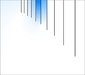
Colour plots of $|\phi (x,z)|$ for the array parametrised by the submergences reported in table 1 are given in figure 3 at all the frequencies $\omega ^{(n)}$. As expected, the strongest local energy amplification in the graded array for a given frequency occurs in the cavity associated with that fundamental frequency. In results not shown here, this does not occur when waves are incident from the right, which is a consequence of the low transmission of high-frequency waves discussed earlier. Furthermore, the differing scales of the colourbars in figure 3 vary in a non-uniform way, which indicates that the resonant frequencies of the graded array do not perfectly coincide with the frequencies $\omega ^{(n)}$. These frequency shifts are introduced by the method used to design the graded array. Firstly, changing the geometry of a cavity from a pair of identical barriers to a pair of unequally submerged barriers increases its fundamental frequency, provided that the mean submergence of the barriers is kept constant. This effect was shown in figure 2(a). Secondly, the coupling of multiple resonators in the graded array alters the resonant frequencies in a non-transparent way.

Figure 3. Colour plots of the velocity potential $|\phi (x,z)|$ when forced by $0.1$ m waves which are incident from the left of the array of barriers. The frequencies of the incident waves shown here are the desired resonant frequencies, which were used to determine the parameters of the array. Specifically, these frequencies are (a) $\omega =1.6$ s$^{-1}$, (b) $1.5$ s$^{-1}$, (c) $1.4$ s$^{-1}$, (d) $1.3$ s$^{-1}$, (e) $1.2$ s$^{-1}$, ( f) $1.1$ s$^{-1}$, (g) $1.0$ s$^{-1}$, (h) $0.9$ s$^{-1}$ and (i) $0.8$ s$^{-1}$. The position of the strongest local energy amplification moves towards the right as the frequency decreases.

In order to analyse this phenomenon further, we consider the propagation of water waves through an infinite periodic array of uniform vertical barriers. Using the present notation, this is the case where $x^{(n)}=nl$ and $d^{(n)}=d$ for all $n\in \mathbb {Z}$, where $l >0$ and $d\in (0,H)$ are fixed. Our intention is to locally approximate the wave field within a finite graded array of vertical barriers using solutions to the infinitely periodic case, which is reasonable provided that the grading is weak (Bennetts et al. Reference Bennetts, Peter and Craster2019). Infinite periodic arrays of uniform vertical barriers can be studied using Bloch's theorem, which motivates seeking solutions of the form

(2.17)\begin{equation} \phi(x+nl,z) = {\rm e}^{\mathrm{i}qnl}\phi(x,z). \end{equation}

In the above equation we have introduced the unknown Bloch wavenumber $q\in \mathbb {C}$. To compute the corresponding Bloch modes, (2.17) is applied to the horizontal boundary of the unit cell $\{(x,z)|x\in (-l/2,l/2)\mbox { and }z\in (-H,0)\}$, which yields

(2.18a,b)\begin{equation} \phi(l/2,z)= {\rm e}^{\mathrm{i}q l}\phi({-}l/2,z)\quad\mbox{and}\quad \frac{\partial \phi}{\partial x}(l/2,z)= {\rm e}^{\mathrm{i}q l} \frac{\partial \phi}{\partial x}({-}l/2,z). \end{equation}

These quasi-periodic boundary conditions are then solved in conjunction with (2.4a)–(2.4d), where suitable modifications are made so that $x\in (-l/2,l/2)$.

A numerical solution is obtained by solving a generalised eigenvalue problem, which incorporates the scattering matrix for a single vertical barrier (see e.g. Peter & Meylan Reference Peter and Meylan2009). For each frequency $\omega$, propagating Bloch modes (i.e. $q\in \mathbb {R}$) are sought in the irreducible Brillouin zone $q\in [0,{\rm \pi} /l]$. We obtain dispersion curves in the $q{-}\omega$ plane, which form so-called band diagrams. We remark that frequency intervals occupied by the dispersion curves are called passbands, and these frequencies are associated with a propagating mode which can travel through the infinite array without a change in amplitude. The slope of the dispersion curve $\textrm {d}\omega /\textrm {d}q$ determines the group velocity of this propagating mode. The frequency intervals in which there are no real-valued Bloch wavenumbers are called bandgaps. At these frequencies, waves cannot propagate without a change in amplitude.

Some examples of band diagrams with different barrier submergences and spacings are shown in figure 4. In each case, our numerical scheme identifies only one passband and one bandgap. We observe that the fundamental frequency of a pair of barriers with separation $l$ and submergence $d$ is a lower bound of the bandgap. The fundamental frequency decreases as the barriers become deeper, which coincides with the dispersion curves becoming more compressed. This mirrors a similar result found by Bennetts et al. (Reference Bennetts, Peter and Craster2018) for infinite two-dimensional arrays of C-shaped cylindrical resonators. In that setting, the resonant frequency of the isolated resonator is an upper bound of the passband, and the resonance is said to induce the bandgap (Chaplain et al. Reference Chaplain, Pajer, De Ponti and Craster2020). In both cases, the bandgap can be shifted by modifying the resonant substructure of the array.

Figure 4. Dispersion curves for infinite periodic arrays of uniform vertical barriers (solid lines) in which $d=(d^{(n-1)}+d^{(n)})/2$ and $l=l^{(n)}$ for (a) $n=2$, (b) $4$, (c) $6$ and (d) $8$. Here, the values of $d^{(n)}$ and $l^{(n)}$ are those of the graded array shown in figure 3. In each panel, the dotted line shows the dispersion relation (2.8), which is the dispersion curve for unobstructed waves. Notably, the bandgap begins above the fundamental frequency of a pair of barriers with separation $l$ and submergence $d$. These fundamental frequencies, which are represented by dashed lines, are (a) $\omega ^{(n)}=1.5$ s$^{-1}$, (b) $1.3$ s$^{-1}$, (c) $1.1$ s$^{-1}$ and (d) $0.9$ s$^{-1}$.

In the finite array of barriers, the potential surrounding each successive pair of barriers can be understood in terms of the corresponding Bloch problem. In particular, the dispersion curve of the infinite array of barriers with submergence $(d^{(n-1)}+d^{(n)})/2$ and spacing $l^{(n)}$ approximately determines the behaviour in the $n$th cavity for a weakly graded structure, and in this setting it is referred to as the local dispersion curve. Since the fundamental frequencies of the cavities decrease from left to right, the local dispersion curves become more compressed and the frequency interval which supports propagating modes becomes narrower. Thus low-frequency waves propagate further towards the right than high-frequency waves.

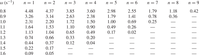
The dispersion curves can also be used to explain the local energy amplification. To demonstrate this, finite difference estimates of the group velocity of the propagating mode are tabulated in table 2 for all cavities and for a range of frequencies. Waves slow down as they propagate through the finite, graded array because the group velocity is a decreasing function of $n$, which attains a minimum before becoming undefined. This minimum typically occurs in the cavity whose fundamental frequency is the frequency of the wave. The wave can only attenuate beyond this point (which is called the turning point by Romero-García et al. (Reference Romero-García, Picó, Cebrecos, Sánchez-Morcillo and Staliunas2013)), since propagation at this frequency is no longer supported by the array. A local energy amplification occurs near the turning point because the propagating mode has a relatively small group velocity, so its energy is localised for a relatively large duration. Moreover, the group velocity is a decreasing function of $\omega$ where it is defined, which means that higher-frequency waves slow down more rapidly than lower-frequency waves and amplify further towards the left, resulting in spatial separation. Thus, graded arrays of vertical barriers give rise to the rainbow-reflection effect.

Table 2. Finite difference estimates of the group velocity (m s$^{-1}$) of waves travelling through the infinite array of barriers with $d=d^{(n-1)}$ and $l=l^{(n)}$, with frequency $\omega$. Dashes (—) are used to denote the absence of a propagating Bloch mode. The group velocity is a decreasing function of both $\omega$ and $n$.

However, the local energy amplification at the turning point is not permanent, so the graded array does not give rise to the rainbow-trapping effect. Because the unit cell of the Bloch problem possesses reflective symmetry, the infinite array supports both left- and right-propagating modes at passband frequencies, which have equal and opposite group velocity. The strong coupling between these modes near the turning point causes the wave to change direction (He et al. Reference He, He and Jin2012; Chaplain et al. Reference Chaplain, Pajer, De Ponti and Craster2020). This coupling is forbidden by rainbow-trapping devices, which can be achieved through the use of certain asymmetric substructures (Chaplain et al. Reference Chaplain, Pajer, De Ponti and Craster2020). Since transmission by the array of barriers is negligible, the left-travelling wave originating at the turning point reflects all of the incident energy. In the following section, we introduce a loss-inducing mechanism into the model, which will allow the localised energy to be absorbed within the structure rather than being reflected.

3.1. Preliminaries

We adapt the problem considered in § 2 by introducing $N$ rigid rectangular floating bodies, or ‘pistons’, which completely occupy the horizontal gap between each adjacent pair of barriers. The pistons are restricted to move vertically in heave and are less dense than the fluid. Further, the density of each piston is $\rho _A^{(n)}/\delta ^{(n)}$, where $\rho _A^{(n)}$ is the area density of the piston with respect to the wetted surface and $\delta ^{(n)}$ is the thickness. The motion of each piston is governed by a damping term proportional to the piston's vertical velocity, with the damping coefficient denoted $\mu ^{(n)}$. A schematic of the geometry of this problem is given in figure 5.

Figure 5. Schematic of the multiple piston cavity problem. Viscous damping is symbolised by dashpots.

We assume that pistons are undergoing small, time-harmonic oscillations about their equilibria. This implies that the submergence of the bottom face of each piston is

(3.1)\begin{equation} z={{\rm Re}}(s^{(n)}\, {\rm e}^{-\mathrm{i}\omega t})-D^{(n)},\end{equation}

where $s^{(n)}$ and $D^{(n)}=\rho _A^{(n)}/\rho$ are the complex amplitude and the equilibrium submergence of the $n$th piston respectively. Here, $\rho$ is the density of the fluid. The relevant forces which govern the dynamics of the pistons are due to hydrostatic pressure, hydrodynamic pressure, gravity and viscous damping. After some algebra, the linearised equations of motion can be stated as

(3.2)\begin{equation} -\omega^{2}\rho_A^{(n)}l^{(n)}s^{(n)}-\mathrm{i}\omega\mu^{(n)} s^{(n)}+\rho g l^{(n)}s^{(n)}=\mathrm{i}\omega\rho \int_{x^{(n-1)}}^{x^{(n)}}\phi(x,-D^{(n)})\,{\rm d} x,\end{equation}

where $l^{(n)}=x^{(n)}-x^{(n-1)}$ (Wehausen Reference Wehausen1971).

We redefine the subregions $\varOmega ^{(n)}$ to be the sets of points beneath the $n$th piston when at equilibrium, that is, $\varOmega ^{(n)} = \{(x,z)|x\in (x^{(n-1)},x^{(n)})\textrm { and }z\in (-H,-D^{(n)})\}$ for all $n\in \{1,\ldots,N\}$. The definitions of $\varOmega ^{(0)}$ and $\varOmega ^{(N+1)}$ are unchanged. The velocity potential of the fluid $\phi$ satisfies the boundary value problem given by (2.4a), (2.4b), (2.4d) and the additional conditions

(3.3a)$$\begin{gather} \partial_z\phi=\frac{\omega^{2}}{g}\phi \quad \text{for } z=0 \text{ and }x\in(-\infty,x^{(0)})\cup(x^{(N)},\infty), \end{gather}$$

(3.3b)$$\begin{gather}\partial_z\phi={-}\mathrm{i}\omega s^{(n)}\quad \mbox{where }x\in(x^{(n-1)},x^{(n)})\text{ and }z={-}D^{(n)}. \end{gather}$$

The potential is also subject to (2.5a,b), (2.6), (2.11) and (2.12).

3.2. Derivation of a system of integral equations

The expansion for the solution given in (2.7) still applies in subregions $\varOmega ^{(0)}$ and $\varOmega ^{(N+1)}$, since there is no piston at the surface of the fluid. In the remaining subregions $\varOmega ^{(n)}$, we express the general solution as the sum of a homogeneous solution $\phi _h^{(n)}$ and a particular solution $\phi _p^{(n)}$, for all $n\in \{1,\ldots,N\}$. The homogeneous solution satisfies (2.4a), (2.4b) and

(3.4)\begin{equation} \partial_z\phi_h^{(n)}(x,-D^{(n)})=0, \end{equation}

for $x\in (x^{(n-1)},x^{(n)})$. These three equations constitute a Sturm–Liouville problem in the $z$ direction. By using separation of variables and choosing an expansion centred at the midpoints of each piston $m^{(n)}=x^{(n-1)}+\frac {1}{2}l^{(n)}$ we obtain

(3.5)\begin{align} \phi_h^{(n)}(x,z)&=A_0^{(n)}+B_0^{(n)}(x-m^{(n)}) +\sum_{m=1}^{\infty} (A_m^{(n)}\cosh(\kappa_m^{(n)} (x-m^{(n)}))\nonumber\\ &\quad +B_m^{(n)}\sinh(\kappa_m^{(n)} (x-m^{(n)}))) \frac{\psi_m^{(n)}(z)}{\cosh\left(\frac{1}{2} \kappa_m^{(n)}l^{(n)}\right)}, \end{align}

where $\kappa _m^{(n)}=m{\rm \pi} /h^{(n)}$ in which $h^{(n)}=H-D^{(n)}$, and the vertical eigenfunctions have been defined as

(3.6)\begin{equation} \psi_m^{(n)}(z)=\sqrt{2}\cos(\kappa_m^{(n)}(z+H)), \end{equation}

for all $m\in \mathbb {N}$. These eigenfunctions satisfy the following orthogonality relation:

(3.7)\begin{equation} \int_{{-}H}^{{-}D^{(n)}}\psi_m^{(n)}(\xi)\psi_p^{(n)}(\xi)\, {{\rm d}} \xi = h^{(n)}\delta_{m p}, \end{equation}

for all $m,p\in \{0\}\cup \mathbb {N}$ and for all $n\in \{1,\ldots,N\}$.

The particular solution $\phi _p^{(n)}$ satisfies (2.4a), (2.4b) and (3.3b). We find a particular solution with the ansatz that $\phi _p^{(n)}$ is quadratic in both $x$ and $z$, which gives

(3.8)\begin{equation} \phi_h^{(n)}(x,z)={-}\frac{\mathrm{i}\omega s^{(n)}}{2h^{(n)}}((z+H)^{2}-(x-m^{(n)})^{2}),\end{equation}

where we have imposed symmetry about the horizontal midpoints $x=m^{(n)}$. This treatment of the inhomogeneous boundary condition is in complete analogy to the solution obtained by Yeung (Reference Yeung1981) for the problem of an oscillating vertical circular cylinder in a fluid of finite depth.

The scattering matrix method presented in § 2.2 cannot be straightforwardly applied to the present problem, since the equations of motion of the pistons and the wave scattering problem must be solved simultaneously. Instead, we solve the system using a fully coupled system of equations. We begin by introducing the auxiliary functions

(3.9)\begin{equation} u^{(n)}(z) = \left\{\begin{array}{ll} \lim_{x\to x_j}\partial_x\phi(x,z) & \mbox{for }z<{-}d^{(n)}\\ 0 & \mbox{for }z\geq{-}d^{(n)}. \end{array}\right. \end{equation}

Applying (2.5b) as $x \to x^{(0)-}$ and $x \to x^{(N)+}$ to (2.7) yields

(3.10)$$\begin{gather} u^{(0)}(z)=\mathrm{i}k_0A_0^{(0)}\psi_0^{(0)}(z)-\sum_{m=0}^{\infty} \mathrm{i}k_mB_m^{(0)}\psi_m^{(0)}(z), \end{gather}$$

(3.11)$$\begin{gather}u^{(N)}(z)={-}\mathrm{i}k_0B_0^{(N+1)}\psi_0^{(0)}(z)+ \sum_{m=0}^{\infty} \mathrm{i}k_mA_m^{(N+1)}\psi_m^{(0)}(z). \end{gather}$$

After referring to (2.10), we obtain the following expressions for the scattered wave coefficients:

(3.12)$$\begin{gather} B_m^{(0)}=A_0^{(0)}\delta_{0m}+\frac{\mathrm{i}}{k_m H} \mathcal{P}^{(0)}(u^{(0)},\psi_m^{(0)}), \end{gather}$$

(3.13)$$\begin{gather}A_m^{(N+1)}=B_0^{(N+1)}\delta_{0m}-\frac{\mathrm{i}}{k_m H} \mathcal{P}^{(N)}(u^{(N)},\psi_m^{(0)}), \end{gather}$$

where $\mathcal {P}^{(n)}(\cdot,\cdot )$ is the real inner product over $(-H,-d^{(n)})$. Similarly, applying (2.5b) as $x \to x^{(n-1)+}$ and $x \to x^{(n)-}$ gives, after referring to (3.5) and (3.8) and invoking (3.7),

(3.14)$$\begin{gather} A_m^{(n)}=\frac{{{\rm coth}}\left(\frac{1}{2}\kappa_m^{(n)}l^{(n)}\right)}{2m{\rm \pi}} (\mathcal{P}^{(n)}(u^{(n)},\psi_m^{(n)})-\mathcal{P}^{(n-1)}(u^{(n-1)},\psi_m^{(n)})), \end{gather}$$

(3.15)$$\begin{gather}B_m^{(n)}=\frac{1}{2m{\rm \pi}}(\mathcal{P}^{(n)}(u^{(n)},\psi_m^{(n)}) +\mathcal{P}^{(n-1)}(u^{(n-1)},\psi_m^{(n)})). \end{gather}$$

Then, applying (2.5a) as $x\to x^{(n)}$ for all $n\in \{0,\ldots,N\}$ and using (3.12), (3.13), (3.14) and (3.15), we obtain the following system of integral equations:

(3.16)\begin{align} &\int_{{-}H}^{{-}d^{(0)}}(K^{(0)}(z,\xi)+K^{(1)}(z,\xi))u^{(0)}(\xi)\, {{\rm d}} \xi-\int_{{-}H}^{{-}d^{(1)}}L^{(1)}(z,\xi)u^{(1)}(\xi)\, {{\rm d}} \xi \nonumber\\ &\quad +\frac{\mathrm{i}\omega s^{(1)}}{2h^{(1)}}((z+H)^{2}-\frac{1}{4}(l^{(1)})^{2})-A_0^{(1)} +\frac{1}{2}B_0^{(1)}l^{(1)}={-}2A_0^{(0)}\psi_0^{(0)}(z), \end{align}

(3.17)\begin{align} &-\int_{{-}H}^{{-}d^{(n-1)}}L^{(n)}(z,\xi)u^{(n-1)}(\xi)\, {{\rm d}} \xi+\int_{{-}H}^{{-}d^{(n)}}(K^{(n)}(z,\xi)+K^{(n+1)}(z,\xi))u^{(n)}(\xi)\, {{\rm d}} \xi\nonumber\\ &\quad -\int_{{-}H}^{{-}d^{(n+1)}}L^{(n+1)}(z,\xi)u^{(n+1)}(\xi)\, {{\rm d}} \xi+\frac{\mathrm{i}\omega}{2}\left(\frac{s^{(n+1)}}{h^{(n+1)}} \left((z+H)^{2}-\frac{1}{4}(l^{(n+1)})^{2}\right)\right.\nonumber\\ &\quad \left.-\frac{s^{(n)}}{h^{(n)}}\left((z+H)^{2}-\frac{1}{4}(l^{(n)})^{2}\right) \right)+A_0^{(n)}+\frac{1}{2}B_0^{(n)}l^{(n)}-A_0^{(n+1)} +\frac{1}{2}B_0^{(n+1)}l^{(n+1)}=0, \end{align}

(3.18)\begin{align} &-\int_{{-}H}^{{-}d^{(N-1)}}L^{(N)}(z,\xi)u^{(N-1)}(\xi)\, {{\rm d}} \xi+\int_{{-}H}^{{-}d^{(N)}}(K^{(N)}(z,\xi)+K^{(0)}(z,\xi))u^{(N)}(\xi)\, {{\rm d}} \xi\nonumber\\ &\quad -\frac{\mathrm{i}\omega s^{(N)}}{2h^{(N)}}\left((z+H)^{2}-\frac{1}{4}(l^{(N)})^{2}\right)+A_0^{(N)} +\frac{1}{2}B_0^{(N)}l^{(N)}=2B_0^{(N+1)}\psi_0^{(0)}(z), \end{align}

where (3.17) holds for all $n\in \{1,\ldots,N-1\}$ and we have defined the integral kernels

(3.19)$$\begin{gather} K^{(0)}(z,\xi)=\sum_{m=0}^{\infty} \frac{\mathrm{i}}{k_mH} \psi_m^{(0)}(z)\psi_m^{(0)}(\xi), \end{gather}$$

(3.20)$$\begin{gather}K^{(n)}(z,\xi)=\sum_{m=1}^{\infty} \frac{{{\rm coth}}(\kappa_m^{(n)}l^{(n)})}{m {\rm \pi}}\psi_m^{(n)}(z)\psi_m^{(n)}(\xi), \end{gather}$$

(3.21)$$\begin{gather}L^{(n)}(z,\xi)=\sum_{m=1}^{\infty} \frac{\operatorname{csch}(\kappa_m^{(n)}l^{(n)})}{m {\rm \pi}}\psi_m^{(n)}(z)\psi_m^{(n)}(\xi). \end{gather}$$

3.3. Numerical solution using a Galerkin method

To find an approximate solution to the system of integral equations, we first suppose that for each $n=0,\ldots,N$, the auxiliary function $u^{(n)}$ can be expanded in terms of an appropriately chosen basis $\{v_j^{(n)}:(-H,-d^{(n)})\to \mathbb {C}|j\in \mathbb {N}\}$ over the interval $(-H,-d^{(n)})$. We then approximate each auxiliary function $u^{(n)}$ by

(3.22)\begin{equation} u^{(n)}(z) \approx \begin{cases} \displaystyle\sum_{j=1}^{M_{{aux}}} c_j^{(n)}v_j^{(n)}(z) & \mbox{for }z<{-}d^{(n)}\\ 0 & \mbox{for }z\geq{-}d^{(n)}, \end{cases} \end{equation}

where we have truncated each expansion at some sufficiently large $M_{{aux}}\in \mathbb {N}$.

After substitution of (3.22) into the system (3.16)–(3.18), we multiply each expression by $v_p^{(n)}(z)$, for some $p\in \{1,\ldots,M_{{aux}}\}$. Here, $n\in \{0,\ldots,N\}$ is the index of the barrier associated with each integral equation. For instance, (3.16) was derived by applying (2.5a) at $x^{(0)}$, so this expression is multiplied by $v_p^{(0)}(z)$ following substitution of (3.22). Integrating each of these expressions with respect to $z$ over $(-H,-d^{(n)})$ subsequently yields the following linear system of equations:

(3.23)\begin{align} &\sum_{m=0}^{\infty}\mathcal{U}_{mp}^{(0)}\mathcal{K}_{m}^{(0)}\sum_{j=1}^{M_{{aux}}} \mathcal{U}_{mj}^{(0)}c_j^{(0)}+\sum_{m=1}^{\infty}\mathcal{V}_{mp}^{(1)} \left(\mathcal{K}_{m}^{(1)}\sum_{j=1}^{M_{{aux}}} \mathcal{V}_{mj}^{(1)}c_j^{(0)}-\mathcal{L}_{m}^{(1)} \sum_{j=1}^{M_{{aux}}}\mathcal{U}_{mj}^{(1)}c_j^{(1)}\right)\nonumber\\ &\quad +\frac{\mathrm{i}\omega s^{(1)}}{2h^{(1)}}\left(\zeta_p^{(1)}-\frac{1}{4}(l^{(1)})^{2}\gamma_{p}^{(1)}\right) -A_0^{(1)}\gamma_{p}^{(1)} +\frac{1}{2}B_0^{(1)}l^{(1)}\gamma_{p}^{(1)}={-}2\mathcal{U}_{0p}^{(0)}A_0^{(0)}, \end{align}

(3.24)\begin{align} &-\sum_{m=1}^{\infty} \mathcal{U}_{mp}^{(n)}\left(\mathcal{L}_{m}^{(n)} \sum_{j=1}^{M_{{aux}}}\mathcal{V}_{mj}^{(n)}c_j^{(n-1)}- \mathcal{K}_{m}^{(n)}\sum_{j=1}^{M_{{aux}}}\mathcal{U}_{mj}^{(n)}c_j^{(n)}\right)\nonumber\\ &\quad +\sum_{m=1}^{\infty} \mathcal{V}_{mp}^{(n+1)}\left(\mathcal{K}_{m}^{(n+1)} \sum_{j=1}^{M_{{aux}}}\mathcal{V}_{mj}^{(n+1)}c_j^{(n)}-\mathcal{L}_{m}^{(n+1)} \sum_{j=1}^{M_{{aux}}}\mathcal{U}_{mj}^{(n+1)}c_j^{(n+1)}\right)\nonumber\\ &\quad +\frac{\mathrm{i}\omega}{2}\left(\frac{s^{(n+1)}}{h^{(n+1)}} \left(\zeta_p^{(n)}-\frac{1}{4}(l^{(n+1)})^{2} \gamma_{p}^{(n)}\right)- \frac{s^{(n)}}{h^{(n)}}\left(\zeta_p^{(n)}-\frac{1}{4}(l^{(n)})^{2} \gamma_{p}^{(n)}\right)\right)\nonumber\\ &\quad+A_0^{(n)} \gamma_{p}^{(n)} +\frac{1}{2}B_0^{(n)}l^{(n)} \gamma_{p}^{(n)}-A_0^{(n+1)} \gamma_{p}^{(n)} +\frac{1}{2}B_0^{(n+1)}l^{(n+1)} \gamma_{p}^{(n)}=0, \end{align}

(3.25)\begin{align} &-\sum_{m=1}^{\infty} \mathcal{U}_{mp}^{(N)}\mathcal{L}_{m}^{(N)}\sum_{j=1}^{M_{{aux}}} \mathcal{V}_{mj}^{(N)}c_j^{(N-1)}+\sum_{m=1}^{\infty} \mathcal{U}_{mp}^{(N)}\mathcal{K}_{m}^{(N)}\sum_{j=1}^{M_{{aux}}} \mathcal{U}_{mj}^{(N)}c_j^{(N)}\nonumber\\ &\quad +\sum_{m=0}^{\infty} \mathcal{V}_{mp}^{(N+1)}\mathcal{K}_{m}^{(0)}\sum_{j=1}^{M_{{aux}}} \mathcal{V}_{mj}^{(N+1)}c_j^{(N)}-\frac{\mathrm{i}\omega s^{(N)}}{2h^{(N)}}\left( \zeta_{p}^{(N)}-\frac{1}{4}(l^{(N)})^{2} \gamma_{p}^{(N)}\right)\nonumber\\ &\quad +A_0^{(N)} \gamma_{p}^{(N)} +\frac{1}{2}B_0^{(N)}l^{(N)} \gamma_{p}^{(N)}=2 B_0^{(N+1)}\mathcal{V}_{0p}^{(N+1)}, \end{align}

where (3.24) holds for all $n\in \{1,\ldots,N-1\}$ and we have defined

(3.26a––c)\begin{equation} \mathcal{K}_{m}^{(0)}=\frac{\mathrm{i}}{k_m H},\quad \mathcal{K}_{m}^{(n)}=\frac{{{\rm coth}}(\kappa_m^{(n)}l^{(n)})}{m{\rm \pi}},\quad \mathcal{L}_{m}^{(n)}=\frac{\operatorname{csch}(\kappa_m^{(n)}l^{(n)})}{m{\rm \pi}}. \end{equation}

Additionally, we have defined

(3.27a,b)$$\begin{gather} \mathcal{U}^{(0)}_{mj}=\mathcal{P}^{(0)}(\psi_m^{(0)},v_j^{(0)}), \quad \mathcal{V}^{(N+1)}_{mj}=\mathcal{P}^{(N)}(\psi_m^{(0)},v_j^{(N)}), \end{gather}$$

(3.28a,b)$$\begin{gather}\mathcal{U}^{(n)}_{mj}=\mathcal{P}^{(n)}(\psi_m^{(n)},v_j^{(n)}),\quad \mathcal{V}^{(n)}_{mj}=\mathcal{P}^{(n-1)}(\psi_m^{(n)},v_j^{(n-1)}), \end{gather}$$

(3.29a,b)$$\begin{gather}\gamma_{j}^{(n)}=\int_{{-}H}^{{-}d^{(n)}}v_j^{(n)}(\xi)\, {{\rm d}} \xi, \quad \zeta_j^{(n)}=\int_{{-}H}^{{-}d^{(n)}}(\xi+H)^{2}v_j^{(n)} (\xi)\, {{\rm d}} \xi. \end{gather}$$

The singularities at $(x^{(n)},-d^{(n)})$ motivate the following choice of basis functions:

(3.30)\begin{equation} v_j^{(n)}(\xi) = \frac{2({-}1)^{j-1}}{{\rm \pi} \sqrt{(H-d^{(n)})^{2}-(H+\xi)^{2}}}T_{2(j-1)} \left(\frac{H+\xi}{H-d^{(n)}}\right), \end{equation}

in which $T_n$ is the Chebyshev polynomial of the first kind of degree $n$. This basis was first introduced by Porter & Evans (Reference Porter and Evans1995) to solve the scattering of linear waves by a single surface-piercing barrier. By using (1.10.2) in Bateman (Reference Bateman1954), the integrals in (3.27a,b) and (3.28a,b) can be evaluated as

(3.31)\begin{equation} \left.\begin{array}{c} \mathcal{U}_{mj}^{(0)}=({-}1)^{j-1}\beta_{m}^{{-}1/2} I_{2(j-1)}(k_{m}(H-d^{(0)})),\\[5pt] \mathcal{V}_{mj}^{(N+1)}=({-}1)^{j-1}\beta_{m}^{{-}1/2} I_{2(j-1)}(k_{m}(H-d^{(N)})),\\[3pt] \mathcal{U}_{mj}^{(n)}=\sqrt{2}J_{2(j-1)}(\kappa_m^{(n)}(H-d^{(n)})),\\[5pt] \mathcal{V}_{mj}^{(n)}=\sqrt{2}J_{2(j-1)}(\kappa_m^{(n)}(H-d^{(n-1)})), \end{array}\right\} \end{equation}

where $J_n$ is the Bessel function of the first kind of order $n$ and $I_n$ is the corresponding modified Bessel function. Furthermore, by applying the symmetry and orthogonality of the even Chebyshev polynomials, the integrals in (3.29a,b) can be evaluated as

(3.32)\begin{equation} \gamma_{j}^{(n)}=\delta_{1j}\quad\mbox{and}\quad \zeta_j^{(n)}=\frac{(H-d^{(n)})^{2}}{4}\begin{cases} 2 & j=1\\ -1 & j=2\\ 0 & j\geq 3. \end{cases} \end{equation}

Equations (3.23), (3.24) and (3.25) form a linear system of $(N+1)M_{{aux}}$ equations with $(N+1)M_{{aux}}+3N$ unknowns. To obtain a further $2N$ equations, we once again apply (2.5b) as $x \to x^{(n-1)+}$ and $x \to x^{(n)-}$. However, in contrast to the derivation of (3.14) and (3.15), we use the fact that $\psi _m^{(n)}$ is orthogonal to the constant function $1$ for all $m\in \mathbb {N}$. After referring to (3.29a,b), we have

(3.33)$$\begin{gather} \sum_{j=1}^{M_{{aux}}}\gamma_{j}^{(n-1)}c_j^{(n-1)}+ \frac{\mathrm{i}\omega s^{(n)}l^{(n)}}{2}-B_0^{(n)}h^{(n)}=0, \end{gather}$$

(3.34)$$\begin{gather}\sum_{j=1}^{M_{{aux}}}\gamma_{j}^{(n)}c_j^{(n)}- \frac{\mathrm{i}\omega s^{(n)}l^{(n)}}{2}-B_0^{(n)}h^{(n)}=0, \end{gather}$$

for $n\in \{1,\ldots,N\}$.

The remaining $N$ equations are derived from the equations of motion of the pistons (3.2). The integral of the hydrodynamic pressure is evaluated by invoking symmetry about ${x=m^{(n)}}$, then expressed in terms of the coefficients of the auxiliary functions by referring to (3.14), (3.22) and (3.28a,b):

(3.35)\begin{align} &\int_{x^{(n-1)}}^{x^{(n)}}\phi(x,-D^{(n)}){{\rm d} x}={-}\frac{\mathrm{i}\omega s^{(n)}}{2}h^{(n)}l^{(n)}+\frac{\mathrm{i}\omega s^{(n)}(l^{(n)})^{3}}{24~h^{(n)}}+l^{(n)}A_0^{(n)}\nonumber\\ &\quad +\frac{\sqrt{2}h^{(n)}}{{\rm \pi}^{2}} \sum_{m=1}^{\infty}\frac{({-}1)^{m}}{m^{2}}\left(\sum_{j=1}^{M_{{aux}}} \mathcal{U}_{mj}^{(n)}c_j^{(n)}-\sum_{j=1}^{M_{{aux}}} \mathcal{V}_{mj}^{(n)}c_j^{(n-1)}\right). \end{align}

After some rearrangement, substitution of (3.1) and (3.35) into (3.2) yields

(3.36)\begin{equation} \sigma^{(n)}s^{(n)}-\mathrm{i}\omega\rho l^{(n)}A_0^{(n)}-\frac{\mathrm{i}\omega\rho\sqrt{2}h^{(n)}}{{\rm \pi}^{2}} \sum_{m=1}^{\infty}\frac{({-}1)^{m}}{m^{2}}\left(\sum_{j=1}^{M_{{aux}}} \mathcal{U}_{mj}^{(n)}c_j^{(n)}-\sum_{j=1}^{M_{{aux}}} \mathcal{V}_{mj}^{(n)}c_j^{(n-1)}\right)=0, \end{equation}

where we have defined

(3.37)\begin{equation} \sigma^{(n)}=\rho_A^{(n)}l^{(n)}\omega^{2}+\rho g l^{(n)} -\frac{\omega^{2}\rho h^{(n)}l^{(n)}}{2}+\frac{\omega^{2}\rho(l^{(n)})^{3}}{24h^{(n)}} -\mathrm{i}\omega\mu^{(n)}.\end{equation}

Finally, we truncate the infinite sums in (3.23), (3.24) and (3.25) after $M_{{ker}}\sim 1000$ terms, then combine them with (3.33), (3.34) and (3.37) to obtain a matrix equation of dimension $M_{{aux}}(N+1)+3N$. This allows us to simultaneously solve for the coefficients of the auxiliary functions $c_j^{(n)}$ for all $n\in \{0,\ldots,N\}$ and $j\in \{1,\ldots,M_{{aux}}\}$, as well as the quantities $A_0^{(n)}$, $B_0^{(n)}$ and $s^{(n)}$ for all $n\in \{1,\ldots,N\}$. The size of $M_{{aux}}$ must be chosen in accordance with $M_{{ker}}\sim 1000$. By choosing $M_{{ker}}=1000$ and $M_{{aux}}=50$, we obtain four-digit accuracy in the unknown coefficients $R$, $T$ and $s^{(n)}$. The convergence properties of this class of Galerkin methods are discussed in more detail by Linton & McIver (Reference Linton and McIver2001).

The unknown wave amplitudes in regions $\varOmega ^{(0)}$ and $\varOmega ^{(N+1)}$ can then be recovered by substituting (3.22) into (3.12) and (3.13). Referring to (3.27a,b) then gives

(3.38a,b)\begin{equation} B_m^{(0)}=A_0^{(0)}\delta_{0m}+\mathcal{K}_{m}^{(0)}\sum_{j=1}^{M_{{aux}}} \mathcal{U}^{(0)}_{mj}c_j^{0}\quad\mbox{and}\quad A_m^{(N+1)}=B_0^{(N+1)}\delta_{0m}-\mathcal{K}_{m}^{(0)} \sum_{j=1}^{M_{{aux}}}\mathcal{V}^{(N+1)}_{mj}c_j^{N}. \end{equation}

Similarly, the remaining unknown coefficients can be recovered after additionally referring to (3.14) and (3.15):

(3.39)$$\begin{gather} A_m^{(n)}=\frac{{{\rm coth}}(\kappa_m^{(n)}l^{(n)}/2)}{2m{\rm \pi}} \left(\sum_{j=1}^{M_{{aux}}}\mathcal{U}_{mj}^{(n)}c_j^{(n)}- \sum_{j=1}^{M_{{aux}}}\mathcal{V}_{mj}^{(n)}c_j^{(n-1)}\right), \end{gather}$$

(3.40)$$\begin{gather}B_m^{(n)}=\frac{1}{2m{\rm \pi}}\left(\sum_{j=1}^{M_{{aux}}} \mathcal{U}_{mj}^{(n)}c_j^{(n)}+\sum_{j=1}^{M_{{aux}}} \mathcal{V}_{mj}^{(n)}c_j^{(n-1)}\right). \end{gather}$$

4.1. Absorption by a single cavity

We first consider absorption by a single cavity absorber (SCA), here defined as a single piston surrounded by a pair of barriers. When the two barriers are identical, an established theoretical result implies that the maximum value of absorption is $\alpha =0.5$ (Budal & Falnes Reference Budal and Falnes1975; Evans Reference Evans1976; Mei Reference Mei1976; Newman Reference Newman1977). For any given frequency, this maximum can be attained by tuning the damping coefficient of the piston and the submergence of the barriers. This tuning is simplified by fixing $l^{(1)}=d^{(0)}/5$ and $\rho _A^{(1)}=500$ kg m$^{-2}$. The parameters which maximise absorption for the frequencies considered in § 2.3 are presented in table 3, where we use a tilde to distinguish parameters that relate to SCAs. We observe that the submergence depths are nearly identical to those in table 1, which were obtained by maximising the time-average power of the free-surface oscillations. This is because the fundamental resonance considered in § 2.3 is essentially a vertical fluid motion between the barriers, which is the fluid motion that maximises energy absorption by a heaving piston.

Table 3. The optimised parameters of a SCA which maximise absorption at $\omega ^{(n)}$, i.e. $\alpha (\omega ^{(n)})=0.5$ is attained.

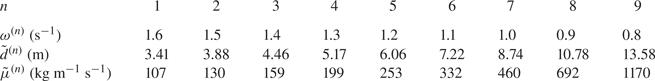
We remark that larger values of $\alpha$ can be attained when $d^{(1)}>d^{(0)}$. Perfect absorption (i.e. $\alpha =1$) occurs when the wave radiated by the piston destructively interferes with the scattered wave, which is impossible for a symmetric device oscillating in one mode of motion (see Falnes (Reference Falnes2002) for more details). However, in the limiting case where $d^{(1)}=H$, the scattered wave propagates in one direction only as no transmission is allowed. This implies that complete destructive interference of the scattered wave by the radiated wave produced by a heave-restricted piston is possible. This limiting case is analogous to the oscillating water columns positioned against a wall considered by Evans & Porter (Reference Evans and Porter1995), where perfect absorption at a given frequency was achieved.

4.2. Optimised absorption at $N$ frequencies

Consider now an array of absorbing cavities whose absorption spectrum has maxima at the $N=9$ prescribed frequencies considered in § 4.1. We construct this array by modifying the algorithm which was used by Jiménez et al. (Reference Jiménez, Romero-García, Pagneux and Groby2017) to design an acoustic RA. The algorithm is a sequence of optimisation problems, whereby the size of the device and the set of frequencies at which absorption is maximised both increase with each iteration. The details of the algorithm are provided in the following paragraph.

For $n$ iteratively incrementing from 1 to $N$, we maximise $\sum _{j=1}^{n} \alpha (\omega ^{(N-j+1)})$ for a device consisting of $n$ cavities, by tuning $d_n^{(j)}$ for $j\in \{0,\ldots,n\}$, and $\mu _n^{(j)}$ for $j\in \{1,\ldots,n\}$. Here, the subscript $n$ refers to the stage of the iteration. The optimisation is performed while fixing ${l_n^{(j)}=(d_n^{(j-1)}+d_n^{(j)})/10}$ for $j\in \{1,\ldots,n\}$, and with the constraints ${\tilde {d}^{(N-n)}< d_n^{(0)}<\dots < d_n^{(n)}<0.8H}$. When $n=N$, these constraints instead become ${2D^{(0)}< d_N^{(0)}<\dots < d_N^{(N)}<0.8H}$. For $n=1$ the initial guesses of the parameters are $d_n^{(0)}=d_n^{(1)}=\tilde {d}^{(N)}$ and $\mu _n^{(1)}=\tilde {\mu }^{(N)}$. At each subsequent stage $n>1$, we initialise the optimisation with ${d_n^{(0)}=\tilde {d}^{(N-n+1)}}$, ${d_n^{(j)}=d_{n-1}^{j-1}}$ for $j\in \{1,\ldots,n\}$, $\mu _n^{(1)}=\tilde {\mu }^{(N-n+1)}$ and $\mu _n^{(j)}=\mu _{n-1}^{(j-1)}$ for $j\in \{2,\ldots,n\}$. In other words, a new cavity which maximises absorption near $\omega ^{(N-n+1)}$ is added to the left of the array constructed during step $n-1$.

The absorption spectra of all of the intermediate devices obtained by this process are given in figure 6, and the parameters of the final device with $n=9$ cavities are given in table 4. As desired, we find that the peaks of the spectra of all intermediate devices coincide with the prescribed frequencies. In analysis not presented here, we find that at the $j$th peak of each spectrum, the largest contribution to absorption is by the $(n-j+1)$th piston. For the final device, we obtain $\alpha (\omega ^{(j)})>0.98$ for $j\in \{1,\ldots,N-1\}$. The constraint that $d^{(N)}<0.8H$ (which was imposed to ensure the solution converges rapidly) hinders absorption at the lowest frequency, where we obtain $\alpha (\omega ^{(N)})\approx 0.93$. In contrast, Jiménez et al. (Reference Jiménez, Romero-García, Pagneux and Groby2017) were able to obtain an acoustic device for which $\alpha =1$ at all $N$ frequencies because the viscothermal energy loss mechanism included in their model is less restrictive. We also observe that the peaks of the spectrum in figure 6(i) become increasingly sharp as $\omega$ increases. As a consequence, absorption becomes increasingly lower in the intervals between the prescribed frequencies. Our next task is to rectify this by using a broadband absorption metric to design a RA, whose absorption spectrum remains close to $1$ over the entire interval $[\omega ^{(N)},\omega ^{(1)}]$.

Figure 6. Absorption spectra of the devices obtained using the steps outlined in § 4.2, which is a modification of that used by Jiménez et al. (Reference Jiménez, Romero-García, Pagneux and Groby2017). The frequencies at which absorption is maximised at each stage of the algorithm are denoted by vertical dotted lines. As desired, the peaks of the spectra coincide with the desired peaks of absorption.

Table 4. Parameters of the device obtained using the modified algorithm of Jiménez et al. (Reference Jiménez, Romero-García, Pagneux and Groby2017). The absorption spectrum of this device is shown in figure 6(i).

4.3. Optimised broadband absorption

Using a similar metric to Jiménez et al. (Reference Jiménez, Romero-García, Pagneux and Groby2017), we quantify the broadband performance of the RA as the average value of $\alpha$ over the interval $[\omega ^{(N)},\omega ^{(1)}]$, i.e.

(4.2)\begin{equation} E=\frac{1}{\omega^{(1)}-\omega^{(N)}}\int_{\omega^{(N)}}^{\omega^{(1)}} \alpha(\omega)\, {{\rm d}} \omega. \end{equation}

It is clear that $E\in [0,1]$. Naively, we can increase $E$ by increasing the length of the cavities, since this decreases the $Q$-factors of the resonant peaks and allows them to overlap more. Broadband performance can also be increased by adding more appropriately tuned cavities to the RA (i.e. increasing $N$), since this increases the number of absorption peaks in a given interval. Both of these avenues to increasing $E$ also increase the total length of the RA given by $L=\sum _{n=1}^{N} l^{(n)}$, which is undesirable due to practical considerations. This motivates the present problem of maximising $E$ while constraining $L$, where we will fix $N=9$.

The maximisation of $E$ is conducted by simultaneously tuning the parameters $d^{(n)}$, $\mu ^{(n)}$ and $l^{(n)}$ over a bounded feasible set which is defined by inequality constraints. Specifically, we require that $L<\lambda _{0.8}/5$, where $\lambda _{0.8}\approx 86.4$ m is the wavelength of a plane wave with frequency $\omega ^{(N)}=0.8$ s$^{-1}$. We also require that $l^{(n)}$ and $\mu ^{(n)}$ are increasing, that $2D^{(1)}< d^{(0)}<\cdots < d^{(N)}<0.8H$ and that $\mu ^{(n)}<2\tilde {\mu }^{(n)}$ for all $n\in \{1,\ldots,9\}$. The resulting constrained optimisation problem is then solved using the MATLAB routine fmincon. In preliminary tests, the introduction of constraints greatly reduced the runtime of the optimisation algorithm by reducing the number of iterations required to achieve convergence. The numerical evaluation of the objective function $E$ is performed using trapezoidal quadrature. The initial guess is the device with $9$ cavities obtained in § 4.2, which has an absorption peak at $9$ discrete frequencies and for which $E\approx 0.787$. In particular, we remark that this initial guess satisfies the constraints. The RA which results from this optimisation procedure is a local maximiser of $E$, but should not be considered a global maximiser.

The parameters of the optimised RA, which attains a value of $E\approx 0.982$, are given in table 5, and its absorption spectrum is shown in figure 7. The spectrum is predictably flat over the interval $[0.8,1.6]$ s$^{-1}$, and we observe two additional absorption peaks at $\omega \approx 1.84$ s$^{-1}$ and $\omega \approx 2.07$ s$^{-1}$. By using (4.1) to partition the area under the absorption spectrum in figure 7, we find that the two additional peaks are the resonances of the third and second cavity respectively. Additionally, the first three pistons have a minor contribution to absorption over the target interval, which can be demonstrated by computing

(4.3)\begin{equation} \frac{1}{\omega^{(1)}-\omega^{(N)}}\sum_{n=1}^{3}\int_{\omega^{(N)}}^{\omega^{(1)}} \alpha^{(n)}(\omega)\, {{\rm d}} \omega<0.035. \end{equation}

However, the RA obtained by removing the first three cavities, with absorption spectrum given by the dotted line in figure 8(a), only attains a value of $E\approx 0.909$. Therefore the purpose of first three cavities cannot be understood in terms of absorption alone.

Figure 7. The absorption spectrum (solid curve) of the optimised RA. The coloured areas under the curve show the relative contribution of each piston to the total absorption by the device.

Table 5. Parameters of the device designed by maximising the broadband performance metric $E$. The absorption spectrum of this device is shown in figure 7.

Figure 8. (a) The absorption spectrum of the optimised RA where the first three cavities have been removed (dotted line) and where the damping coefficients of the first three pistons are changed to zero (solid line). The absorption spectrum of the unaltered RA also shown in figure 7 is included for comparison (dashed line). (b) The absorption spectra of devices (i) (dotted line) and (ii) (solid line) described in the text. As was the case in (a), device (ii) differs from device (i) by the inclusion of three non-absorbing cavities.

Indeed, the primary role of cavities $1$–$3$ is to intensify the local energy amplification in cavities $4$–$9$, which results in greater absorption by the pistons in these cavities. We interpret that this is because the coupling between the incident plane wave and the resonant mode in the cavity where the amplification occurs is strengthened by the inclusion of cavities $1$–$3$. To illustrate this, we consider (i) a SCA with the same parameters as cavity $4$ of the optimised RA and (ii) an array of four cavities consisting of the first four cavities of the optimised RA, but where $\mu ^{(n)}=0$ for $n\in \{1,2,3\}$. Hence both devices contain a single absorbing cavity whose parameters are identical, but device (ii) additionally contains three non-absorbing cavities positioned to the left. Cavities $5$–$9$ have been omitted from both devices in order to simplify their absorption spectra, which are contrasted in figure 8(b). Importantly, the absorption peak of device (ii) is significantly higher than that of device (i), which suggests that the resonant mode in the absorbing cavity of device (ii) is more strongly coupled to the incident plane wave. This coupling occurs sequentially via the propagating Bloch modes of the three non-absorbing cavities, through which the group velocity gradually decreases (recall from § 2.4 that the group velocity of the resonant mode is close to zero). In device (i), the coupling between the plane wave and the resonant mode must occur directly, which evidently results in a less-intense energy amplification. In figure 8(a), this experiment is also conducted without omitting cavities $5$–$9$ (see solid line), so that both of the devices being compared have six identical absorbing cavities. We observe that absorption over $[0.8,1.6]$ s$^{-1}$ is reduced much less by setting the damping coefficient of the first three pistons to zero than by removing the first three cavities. This further demonstrates the important role that cavities $1$–$3$ have in facilitating the transfer of energy from the incident plane wave to pistons $4$–$9$ in the optimised RA. We conclude that the two additional absorption peaks in figure 7 are a by-product of the geometry that cavities $2$ and $3$ must have in order to optimise this energy transfer.