


1. Introduction
The break-up of cylindrical vesicles under external tension has been successfully described by a Rayleigh–Plateau mechanism in direct analogy to the break-up of a liquid jet due to surface tension (Bar-Ziv & Moses Reference Bar-Ziv and Moses1994; Goldstein et al. Reference Goldstein, Nelson, Powers and Seifert1996; Kantsler, Segre & Steinberg Reference Kantsler, Segre and Steinberg2008; Powers Reference Powers2010; Sanborn et al. Reference Sanborn, Oglecka, Kraut and Parikh2013; Boedec, Jaeger & Leonetti Reference Boedec, Jaeger and Leonetti2014; Narsimhan, Spann & Shaqfeh Reference Narsimhan, Spann and Shaqfeh2015; Pal & Khakhar Reference Pal and Khakhar2019). In living cells, a Rayleigh–Plateau instability has further been proposed for fission of mitochondria (Gonzalez-Rodriguez et al. Reference Gonzalez-Rodriguez, Sart, Babataheri, Tareste, Barakat, Clanet and Husson2015) and for blood platelet formation (Bächer, Bender & Gekle Reference Bächer, Bender and Gekle2020).
In contrast to passive systems such as vesicles or liquid jets, living cells can actively produce tensions within their cell membrane (Prost, Jülicher & Joanny Reference Prost, Jülicher and Joanny2015; Salbreux & Jülicher Reference Salbreux and Jülicher2017; Jülicher, Grill & Salbreux Reference Jülicher, Grill and Salbreux2018). These tensions, in turn, are often anisotropic (Rauzi et al. Reference Rauzi, Verant, Lecuit and Lenne2008; Salbreux, Prost & Joanny Reference Salbreux, Prost and Joanny2009; Mayer et al. Reference Mayer, Depken, Bois, Jülicher and Grill2010; Behrndt et al. Reference Behrndt, Salbreux, Campinho, Hauschild, Oswald, Roensch, Grill and Heisenberg2012; Reymann et al. Reference Reymann, Boujemaa-Paterski, Martiel, Guerin, Cao, Chin, De La Cruz, Thery and Blanchoin2012; Murrell et al. Reference Murrell, Oakes, Lenz and Gardel2015; Blackwell et al. Reference Blackwell, Sweezy-Schindler, Baldwin, Hough, Glaser and Betterton2016; Callan-Jones et al. Reference Callan-Jones, Ruprecht, Wieser, Heisenberg and Voituriez2016; Reymann et al. Reference Reymann, Staniscia, Erzberger, Salbreux and Grill2016; Zhang et al. Reference Zhang, Kumar, Ross, Gardel and de Pablo2018), which has substantial consequences for the Rayleigh–Plateau scenario as we have demonstrated by linear stability analysis and numerical simulations for a fluid interface in Part 1 of this series (Graessel, Bächer & Gekle Reference Graessel, Bächer and Gekle2021): if azimuthal tensions are stronger than axial tensions, the range of unstable wavelengths grows and the most unstable mode shifts towards a shorter wavelength.
Another crucial difference between liquid jets and cell or vesicle membranes is the elastic response of the latter. The elastic response typically consists of independent contributions which can be related to different structural components of the membrane. First, the lipid bilayer induces a resistance to bending as well as area dilatation. Second, biological cells possess a cellular cortex, located directly beneath the lipid bilayer (Alberts et al. Reference Alberts, Johnson, Lewis, Raff, Roberts and Walter2007), in which cross-linked polymers such as spectrin form an elastic network which adds a resistance to shear deformation. Over the last decades, a series of semi-empirical constitutive laws have been shown to fairly accurately describe these resistances. For bending, the Helfrich Hamiltonian (Helfrich Reference Helfrich1973; Guckenberger & Gekle Reference Guckenberger and Gekle2017) is the most widely used description, while for shear and area dilatation the Skalak (Skalak et al. Reference Skalak, Tozeren, Zarda and Chien1973) as well as neo-Hookean laws (Barthès-Biesel, Diaz & Dhenin Reference Barthès-Biesel, Diaz and Dhenin2002; Barthès-Biesel Reference Barthès-Biesel2016; Jaensson & Vermant Reference Jaensson and Vermant2018) have been established. The elasticity is not only important for the regulation of vesicle or cell shape (Fischer Reference Fischer2004; Barthès-Biesel Reference Barthès-Biesel2016; Jelerčič Reference Jelerčič2017), it is further known to drive wrinkling on the vesicle surface (Finken & Seifert Reference Finken and Seifert2006; Li & Sarkar Reference Li and Sarkar2008; Finken, Kessler & Seifert Reference Finken, Kessler and Seifert2011; Dupont et al. Reference Dupont, Salsac, Barthès-Biesel, Vidrascu and Le Tallec2015; Narsimhan et al. Reference Narsimhan, Spann and Shaqfeh2015) and can lead to budding of vesicles (Seifert, Berndl & Lipowsky Reference Seifert, Berndl and Lipowsky1991; Seifert & Lipowsky Reference Seifert, Lipowsky, Lipowsky and Sackmann1995).
A small number of theoretical studies have so far investigated the influence of these elastic properties on the Rayleigh–Plateau instability of vesicles and cells. Bending elasticity has been shown to set a threshold for the tension required to trigger the instability (Nelson, Powers & Seifert Reference Nelson, Powers and Seifert1995; Goldstein et al. Reference Goldstein, Nelson, Powers and Seifert1996; Powers Reference Powers2010; Patrascu & Balan Reference Patrascu and Balan2020). Furthermore, Campelo & Hernández-Machado (Reference Campelo and Hernández-Machado2007) show by simulations that a non-zero curvature in the Helfrich Hamiltonian due to membrane anchoring proteins (Tsafrir et al. Reference Tsafrir, Sagi, Arzi, Guedeau-Boudeville, Frette, Kandel and Stavans2001) is capable of triggering a Rayleigh–Plateau instability. Boedec et al. (Reference Boedec, Jaeger and Leonetti2014) investigate the growth rate and the most unstable wavelength for a general tension with respect to bending elasticity. They show that increasing the bending modulus leads to a smaller range of unstable modes compared to the classical Rayleigh–Plateau regime, where modes grow up to a wavenumber equal to the undeformed tube radius (Rayleigh Reference Rayleigh1878; Drazin & Reid Reference Drazin and Reid2004). Beyond a threshold bending modulus, they find that the instability is suppressed (Boedec et al. Reference Boedec, Jaeger and Leonetti2014). Considering shear elasticity, Hannezo, Prost & Joanny (Reference Hannezo, Prost and Joanny2012) use an energy argument to predict a Rayleigh–Plateau instability of a tissue tube above a critical active tension depending on the Young's modulus of the tissue. Going in the same direction, Berthoumieux et al. (Reference Berthoumieux, Maître, Heisenberg, Paluch, Jülicher and Salbreux2014) derive the Green's function of an elastic membrane subjected to active tension. Both approaches, however, do not lead to the full dispersion relation for the growth of perturbations. To the best of our knowledge, a full linear stability analysis including shear elasticity has so far not been carried out. Furthermore, and most importantly, all the above studies on the Rayleigh–Plateau instability under the influence of bending and shear elasticity consider isotropic tension.
In this paper, motivated by the frequent observation of anisotropic active tensions in cell membranes, we explore the diversity of the Rayleigh–Plateau instability which results from the interplay of tension anisotropy and interface elasticity. We first consider bending elasticity in the framework of the Helfrich model and analytically derive the dispersion relation in the Stokes limit by a linear stability analysis. In addition to the classical scenario with a single wavenumber separating stable from unstable modes, we find that bending elasticity introduces a new restricted regime in which an intermediate range of unstable modes is bounded from above and below by two separate stable ranges. Bending resistance can also lead to a regime where the interface is stable against all perturbations, the onset of which strongly depends on the tension anisotropy. We also provide a detailed investigation of the influence of the reference curvature. We show that the scenario remains qualitatively unchanged when replacing the Stokes by the Euler equation for the fluid dynamics. Next, we consider shear elasticity and area dilatation based on the Skalak law and calculate the corresponding dispersion relation in the Stokes limit. The dominant wavelength is found to increase due to the damping nature of the shear elasticity. Above a critical shear modulus only a stable phase exists, the critical value decreases when strengthening the resistance to area dilatation. While the threshold to the stable phase is independent of tension anisotropy, increasing the latter systematically increases the instability wavelength. Investigating the interplay of bending and shear elasticity, we analyse the resulting dispersion relation and observe a combination of the characteristic features of both effects with strong influence of the tension anisotropy.
We start by introducing the description of a deformable, elastic interface in § 2 which requires a different theoretical basis than the purely viscous interfaces in Reference Graessel, Bächer and GeklePart 1. In § 3 we proceed with the interfacial forces due to bending elasticity based on the Helfrich model and in § 3.1 perform a linear stability analysis which leads to the dispersion relation. Next, we analyse the growing modes and the different regimes induced by the bending elasticity (§ 3.2), followed by the dominant wavelength in § 3.3. In § 3.4 we systematically vary the reference curvature. As a next step we derive the dispersion relation for shear resistance and area dilatation based on the Skalak law and investigate the stability and dominant wavelength under the influence of both Skalak elasticity and tension anisotropy in § 4. Eventually, we combine bending and shear resistance in § 5. We conclude in § 6.
2. Problem set-up: a deformable elastic interface surrounded by fluid
2.1. Differential geometry of a deformable interface
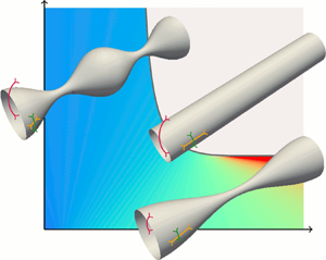
We consider an initially cylindrical elastic interface subjected to an axisymmetric periodic perturbation along its axis, as illustrated in figure 1. In contrast to Reference Graessel, Bächer and GeklePart 1, the elasticity of the interface now requires us to consider the total deformation  $\boldsymbol {u}$ of an interface point from its initial location, and not only the local curvature and velocity. For this we employ the differential geometry (Kreyszig Reference Kreyszig1968) of thin shells as detailed in Green & Zerna (Reference Green and Zerna1954), Deserno (Reference Deserno2015), Salbreux & Jülicher (Reference Salbreux and Jülicher2017) and Bächer & Gekle (Reference Bächer and Gekle2019), whose notation we follow. In the following, we introduce all quantities used in the linear stability analysis.

Figure 1. Cylindrical, elastic interface under periodic perturbation. We consider an axisymmetric interface between an inner, enclosed and an outer, surrounding fluid. The surface of the complex interface is parametrised by  $\boldsymbol {X}(\phi ,z)$, the undeformed reference state (dotted line) is described by $\boldsymbol {X}_0$. The in-plane coordinate vectors which point along the interface are $\boldsymbol {e}_\phi$ and $\boldsymbol {e}_z$, the unit normal vector on the interface $\boldsymbol {n}$ points outwards. In addition to the azimuthal curvature $c_\phi ^\phi$ along $\boldsymbol {e}_\phi$ the perturbation leads to an axial curvature $c_z^z$ along $\boldsymbol {e}_z$.
The undeformed state of the interface is a cylinder with radius  $R_0$ in the radial direction $r$, which is parametrised in cylindrical coordinates by azimuthal angle $\phi$ and axial position $z$
$z$
 \begin{equation} \boldsymbol{X}_0 = \boldsymbol{X}_0 (\phi, z) = R_0 \hat{\boldsymbol{e}}_r + z \hat{\boldsymbol{e}}_z \end{equation}
with the normalised radial  $\hat {\boldsymbol {e}}_r = ( \cos \phi , \sin \phi , 0 )$ and axial coordinate vector $\hat {\boldsymbol {e}}_z = ( 0,0,1 )$. A periodic perturbation along the axis leads to a deformation $\boldsymbol {u}$ of the interface
 \begin{equation} \boldsymbol{u} = \boldsymbol{X} - \boldsymbol{X}_0 = u_r \hat{\boldsymbol{e}}_r + u_z \hat{\boldsymbol{e}}_z, \end{equation}
where we parametrise the deformed interface with varying radius  $R(z) = R_0 + u_r(z)$ by
 \begin{equation} \boldsymbol{X} = \boldsymbol{X} (\phi, z) = \left( \begin{array}{c} R(z) \cos \phi \\ R(z) \sin \phi \\ z + u_z(z) \end{array} \right). \end{equation}
In the following, we consider small amplitude perturbations and therefore keep only terms up to linear order in the deformation (Berthoumieux et al. Reference Berthoumieux, Maître, Heisenberg, Paluch, Jülicher and Salbreux2014; Daddi-Moussa-Ider, Lisicki & Gekle Reference Daddi-Moussa-Ider, Lisicki and Gekle2017). The in-plane coordinate vectors, i.e. the coordinate vectors along the deformed interface, are
 \begin{equation} \boldsymbol{e}_\phi = \frac{\partial}{\partial \phi} \boldsymbol{X} = \left( \begin{array}{c} - R \sin\phi \\ R \cos\phi \\ 0 \end{array} \right),\quad \boldsymbol{e}_z = \frac{\partial}{\partial z} \boldsymbol{X} = \left( \begin{array}{c} R^\prime \cos\phi \\ R^\prime \sin\phi \\ 1 + u_z^\prime \end{array} \right), \end{equation}
with the prime denoting a derivative with respect to  $z$. From the in-plane coordinate vectors the metric on the deformed interface can be calculated (Kreyszig Reference Kreyszig1968) and linearised
 \begin{equation} g_{\alpha\beta} = \boldsymbol{e}_\alpha \cdot \boldsymbol{e}_\beta =\left(\begin{array}{cc} R^2 & 0 \\ 0 & \left( 1+u_z^\prime \right)^2 + R^{\prime2} \\ \end{array} \right) \approx \left( \begin{array}{cc} R_0^2 + 2 R_0 u_r & 0 \\ 0 & 1 + 2 u_z^\prime \end{array}\right),\end{equation}
with  $\alpha ,\beta =\phi ,z$. The inverse metric defined by $g_{\alpha \gamma }g^{\gamma \beta } = \delta _\alpha ^\beta$ takes the form
 \begin{equation} g^{\alpha\beta} = \left(\begin{array}{cc} \dfrac{1}{R^2} & 0 \\ 0 & \dfrac{1}{\left( 1+u_z^\prime \right)^2 + R^{\prime2}} \end{array} \right)\approx \left( \begin{array}{cc} \dfrac{1}{R_0^2} - 2 \dfrac{u_r}{R_0^3} & 0 \\ 0 & 1 - 2 u_z^\prime \end{array} \right). \end{equation}
We obtain the metric on the undeformed interface  $G_{\alpha \beta }$ by setting the deformation to zero
 \begin{equation} G_{\alpha\beta} = \left( \begin{array}{cc} R_0^2 & 0 \\ 0 & 1 \end{array} \right),\quad G^{\alpha\beta} = \left( \begin{array}{cc} \dfrac{1}{R_0^2} & 0 \\ 0 & 1 \end{array} \right). \end{equation}
From the metric the Christoffel symbols can be calculated by
 \begin{equation} \varGamma_{{\alpha\beta}}^\gamma = \tfrac{1}{2} g^{\gamma\delta} \left( \partial_\beta g_{\alpha\delta} + \partial_\alpha g_{\beta\delta} - \partial_\delta g_{\alpha\beta} \right), \end{equation}
where indices occurring twice are summed over according to the Einstein notation. By the use of the Christoffel symbols the covariant derivative of an arbitrary tensor  $t^{\alpha \beta }$ is defined by
 \begin{equation} \nabla_\alpha t^{\beta \gamma} = \partial_\alpha t^{\beta\gamma} + \varGamma^{\beta}_{\alpha\delta} t^{\delta\gamma} + \varGamma^\gamma_{\alpha\delta} t^{\beta\delta}. \end{equation}
The unit normal vector on the interface, which points outwards, can be calculated in linearised form as
 \begin{equation} \boldsymbol{n} = \frac{\boldsymbol{e}_\phi \times \boldsymbol{e}_z}{| \boldsymbol{e}_\phi \times \boldsymbol{e}_z |} \approx \left(\begin{array}{c} \cos\phi \\ \sin\phi \\ -R^\prime \end{array} \right). \end{equation}
The curvature tensor, which is defined by  $c_{\alpha \beta } = - ( \partial _\alpha \boldsymbol {e}_\beta ) \boldsymbol{\cdot} \boldsymbol {n}$, becomes on the deformed interface
 \begin{equation} c_\alpha^\beta \approx \left( \begin{array}{cc} \dfrac{1}{R(z)} & 0 \\ 0 & -R^{\prime\prime} \end{array}\right). \end{equation}
On the undeformed surface the curvature tensor is
 \begin{equation} C_\alpha^\beta = \left( \begin{array}{cc} \dfrac{1}{R_0} & 0 \\ 0 & 0 \end{array}\right). \end{equation}
2.2. Mechanical properties of the interface
The mechanical properties of the interface are (i) the anisotropic interfacial tension and (ii) the resistance to elastic deformations. If in addition interface viscosity is included, we would expect effects similar to those discussed in Reference Graessel, Bächer and GeklePart 1. In general, mechanical properties of the interface are described by the surface stress (Green & Zerna Reference Green and Zerna1954; Barthès-Biesel Reference Barthès-Biesel2016; Guckenberger & Gekle Reference Guckenberger and Gekle2017; Salbreux & Jülicher Reference Salbreux and Jülicher2017; Bächer & Gekle Reference Bächer and Gekle2019), which can be expressed in vector notation as
 \begin{equation} \boldsymbol{t}^\beta = t_\alpha^{\beta}\boldsymbol{e}^\alpha + t_n^\beta \boldsymbol{n}, \end{equation}
with its in-plane components  $t_\alpha ^\beta$ and the normal component $t_ n^\beta$. As introduced above, we split the surface stress into an (i) anisotropic and an (ii) elastic contribution
 \begin{equation} \boldsymbol{t}^\beta = \boldsymbol{t}^\beta_{{aniso}} + \boldsymbol{t}^\beta_{{el}}. \end{equation}
 As discussed in Reference Graessel, Bächer and GeklePart 1, anisotropic interfacial tension can have different origins. In this paper, we focus on biological cells where proteins in the cell cortex produce an active tension, which enters the anisotropic contribution of the surface stress (2.14). A positive active tension accounts for the internal tendency of the cortical protein network to contract. Similar to surface tension triggering the Rayleigh–Plateau instability of a liquid jet (Eggers & Villermaux Reference Eggers and Villermaux2008), such a contractile active tension in the cell cortex can lead to a Rayleigh–Plateau instability of a cell or tissue tube (Hannezo et al. Reference Hannezo, Prost and Joanny2012; Berthoumieux et al. Reference Berthoumieux, Maître, Heisenberg, Paluch, Jülicher and Salbreux2014; Bächer & Gekle Reference Bächer and Gekle2019; Bächer et al. Reference Bächer, Bender and Gekle2020). In contrast to the classical surface tension, however, here, a constitutive law directly prescribes the active, thus interfacial, tension (rather than deriving it from an interfacial energy) (Salbreux & Jülicher Reference Salbreux and Jülicher2017; Bächer & Gekle Reference Bächer and Gekle2019). In analogy to Reference Graessel, Bächer and GeklePart 1, the anisotropic interfacial tension is denoted by  $\gamma ^\phi$ and $\gamma ^z$, distinguishing azimuthal and axial directions, respectively, and it contributes to the surface stress as
 \begin{equation} t^{\beta}_{{aniso}, \alpha } = \left( \begin{array}{cc} \gamma^\phi & 0 \\ 0 & \gamma^z \end{array}\right). \end{equation}
The normal component of the anisotropic surface stress vanishes, i.e.  $t_{{aniso},n}^\beta =0$. We assume that the anisotropic tension is constant along the interface and therefore derivatives of the anisotropic tension vanish, i.e. $\nabla _\alpha t^{\beta \gamma }_{{aniso}} =0$.
In addition to Reference Graessel, Bächer and GeklePart 1, we here consider a resistance to elastic deformations, which splits into the three different contributions due to bending deformation, shear deformation and area dilatation. The surface stress due to elasticity  $\boldsymbol {t}^\alpha _{{el}}$ can be derived from constitutive laws typically defining an energy functional, which covers the elastic properties (Green & Zerna Reference Green and Zerna1954). In the present paper we use the Helfrich law for bending elasticity with the bending modulus $\kappa _{{B}}$ and the Skalak law for shear elasticity with modulus $\kappa _{{S}}$ and area dilatation with modulus $C \kappa _{{S}}$. The corresponding contributions to the surface stress $\boldsymbol {t}^\alpha _{{el}}$ are derived in §§ 3.1 and 4.1, respectively.
We end this section with a discussion of typical values for vesicles and cells. For the active cortical stress values in the range of  $10^{-5}$– $10^{-3}$ N m $^{-1}$ have been reported depending on the cell type (Lomakina et al. Reference Lomakina, Spillmann, King and Waugh2004; Krieg et al. Reference Krieg, Arboleda-Estudillo, Puech, Käfer, Graner, Müller and Heisenberg2008; Tinevez et al. Reference Tinevez, Schulze, Salbreux, Roensch, Joanny and Paluch2009; Bergert et al. Reference Bergert, Chandradoss, Desai and Paluch2012; Fischer-Friedrich et al. Reference Fischer-Friedrich, Hyman, Jülicher, Müller and Helenius2014; Chugh et al. Reference Chugh, Clark, Smith, Cassani, Dierkes, Ragab, Roux, Charras, Salbreux and Paluch2017; Dmitrieff et al. Reference Dmitrieff, Alsina, Mathur and Nédélec2017). Exact values for the anisotropy of the active stress are scattered as well. Mayer et al. (Reference Mayer, Depken, Bois, Jülicher and Grill2010) report a polar tension half the angular tension for an ellipsoidal embryo, Behrndt et al. (Reference Behrndt, Salbreux, Campinho, Hauschild, Oswald, Roensch, Grill and Heisenberg2012) report a factor of 4 in the case of epiboly. Reymann et al. (Reference Reymann, Staniscia, Erzberger, Salbreux and Grill2016) report anisotropy in terms of a nematic order parameter which takes values from $-$0.04 to 0.12. Rauzi et al. (Reference Rauzi, Verant, Lecuit and Lenne2008) consider planar anisotropy from 1 to 4. Typical values for the bending modulus are in a range from $10^{-20}$– $10^{-18}$ Nm (Goldstein et al. Reference Goldstein, Nelson, Powers and Seifert1996; Freund Reference Freund2014; Guckenberger & Gekle Reference Guckenberger and Gekle2017). The shear elasticity of a red blood cell is in the range $10^{-6}$– $10^{-5}$ N m $^{-1}$ (Freund Reference Freund2014) and the Youngs modulus of a tissue tube is approximately $10^4$– $10^{6}$ Pa (Laurent et al. Reference Laurent, Girerd, Mourad, Lacolley, Beck, Boutouyrie, Mignot and Safar1994; Hannezo et al. Reference Hannezo, Prost and Joanny2012). Eventually, the typical radii from vesicles to tissue tubes varies from approximately half a micrometre (Bar-Ziv & Moses Reference Bar-Ziv and Moses1994; Goldstein et al. Reference Goldstein, Nelson, Powers and Seifert1996) to several micrometres (Freund Reference Freund2014) to a millimetre. All in all, this leads to a wide parameter space, which we cover by presenting phase diagrams for a broad range of dimensionless parameters in the following sections.
2.3. Coupling to the surrounding fluid
Due to the presence of the surrounding fluid, in addition to the surface stress, forces from the fluid act on the interface, which are described by the traction jump across the membrane (Pozrikidis Reference Pozrikidis2001; Daddi-Moussa-Ider & Gekle Reference Daddi-Moussa-Ider and Gekle2018)
 \begin{equation} {\rm \Delta} \boldsymbol{f} = {\rm \Delta} f^\alpha \boldsymbol{e}_\alpha + {\rm \Delta} f^n \boldsymbol{n}, \end{equation}
with components parallel to the interface denoted by  ${\rm \Delta} f^\alpha$ and components along the outward pointing normal vector by ${\rm \Delta} f^n$. The traction jump is given by the difference of the three-dimensional ( $i,j=x,y,z$) stress tensors $\sigma _{ij}^{{out}}$, $\sigma _{ij}^{{in}}$ of the outer and inner fluid, respectively, projected onto the normal vector of the interface (Chandrasekharaiah & Debnath Reference Chandrasekharaiah and Debnath2014)
 \begin{equation} {\rm \Delta} f_j = \left(\sigma_{ij}^{{out}} - \sigma_{ij}^{{in}} \right) n_i. \end{equation}
For a Newtonian and incompressible fluid with shear viscosity  $\eta$ the stress tensor is (Chandrasekharaiah & Debnath Reference Chandrasekharaiah and Debnath2014)
 \begin{equation} \boldsymbol{\sigma} = - p \boldsymbol{I} + \eta \left[\left(\boldsymbol{\nabla}\boldsymbol{v} + \left(\boldsymbol{\nabla}\boldsymbol{v}\right)^\textrm{T}\right)\right], \end{equation}
where  $\boldsymbol {v}(\boldsymbol {r},t)$ is the velocity field and $p(\boldsymbol {r},t)$ the pressure of the fluid.
The interface is considered in mechanical equilibrium with the fluid enclosed by the interface and the surrounding fluid. Therefore, interfacial forces derived from the surface stress (2.14) together with the traction jump (2.16) fulfil the force balance equation (Green & Zerna Reference Green and Zerna1954; Barthès-Biesel Reference Barthès-Biesel2016; Salbreux & Jülicher Reference Salbreux and Jülicher2017)
 \begin{equation} \nabla_\beta \boldsymbol{t}^\beta + {\rm \Delta} \boldsymbol{f} = 0. \end{equation}
The interfacial forces acting from the interface onto the fluid are thus given by either the derivative of the surface stress or the negative traction jump and denoted by
 \begin{equation} \boldsymbol{f} \equiv \nabla_\beta \boldsymbol{t}^\beta = - {\rm \Delta} \boldsymbol{f}. \end{equation}
Decomposing the force balance into components parallel and normal to the interface and using (2.14), (2.15) and (2.16) leads to the force balance equations in the form
 \begin{gather} \nabla_{\alpha}^{} t^{\alpha\beta}_{{el}} + c_{\alpha}^{\beta} t^{\alpha}_{{el},n} = -{\rm \Delta} f^{\beta}, \end{gather}
 \begin{gather}\nabla_{\alpha}^{} t^{\alpha}_{{el},n} - c^{}_{\alpha\beta} t^{\alpha\beta}_{{el}} - c^{}_{\alpha\beta} t^{\alpha\beta}_{{aniso}} = - {\rm \Delta} f^n . \end{gather}
In contrast to Reference Graessel, Bächer and GeklePart 1, the interface elasticity causes a traction jump in the tangential component  ${\rm \Delta} f^\beta$ along the interface and, in addition, modifies the normal force balance. For the exact form of the elastic surface stresses we again refer to §§ 3.1 and 4.1. According to the normal component of the force balance equation (2.22) the anisotropic interfacial tension leads to a contribution
 \begin{equation} c^{}_{\alpha\beta} t^{\alpha\beta}_{{aniso}} = \frac{\gamma^z}{R_z} + \frac{\gamma^\phi}{R_\phi}, \end{equation}
which balances the normal component of the traction jump. In the present paper we consider an interior fluid which has the same viscosity as the surrounding fluid.
3. Bending elasticity restricts anisotropic Rayleigh–Plateau instability
3.1. Dispersion relation from the Helfrich Hamiltonian
We now investigate the influence of bending elasticity on the anisotropic Rayleigh–Plateau instability of an interface specifically aiming at the description of vesicle and cell membranes composed of a lipid bilayer. This bilayer resists bending deformations, i.e. changes of the mean curvature  $H$, which is given by half the trace of the curvature tensor (2.11) (Deserno Reference Deserno2015; Daddi-Moussa-Ider et al. Reference Daddi-Moussa-Ider, Lisicki and Gekle2017)
 \begin{equation} H = \tfrac{1}{2} c_\gamma^\gamma = \tfrac{1}{2} \left(c_z^z + c_\phi^\phi\right). \end{equation}
Deformations which lead to a mean curvature  $H$ different from the reference curvature $H_0$ trigger elastic forces. Due to the Gauss–Bonnet theorem the Gaussian curvature does not affect the interface elasticity (Deserno Reference Deserno2015; Daddi-Moussa-Ider et al. Reference Daddi-Moussa-Ider, Lisicki and Gekle2017). The resistance to bending is described by the Helfrich Hamiltonian (Helfrich Reference Helfrich1973; Guckenberger & Gekle Reference Guckenberger and Gekle2017) with the elastic bending modulus $\kappa _{B}$ as a measure of the bending elasticity
 \begin{equation} W^{{HF}} = 2 \kappa_{{B}} (H-H_0)^2. \end{equation}
As detailed above, the bending elasticity contributes to the elastic surface stress  $\boldsymbol {t}^\alpha _{{el}}$ in (2.14). This contribution can be derived from the Helfrich Hamiltonian (3.2) using thin shell theory (Capovilla & Guven Reference Capovilla and Guven2002; Guven Reference Guven2004; Powers Reference Powers2010; Deserno Reference Deserno2015; Guckenberger & Gekle Reference Guckenberger and Gekle2017), which leads to the general form
 \begin{equation} \boldsymbol{t}^\alpha_{{el},{B}} = 2 \kappa_{{B}} \left( H - H_0 \right)^2 g^{\alpha\beta} \boldsymbol{e}_\beta - 2 \kappa_{{B}} \left( H-H_0 \right) c^{\alpha\beta} \boldsymbol{e}_\beta + 2 \kappa_{{B}} \nabla_\beta \left( H-H_0 \right) g^{\alpha\beta} \boldsymbol{n}. \end{equation}
In the following, we explicitly consider the initially cylindrical interface, subjected to a deformation as given by (2.2) and shown in figure 1. Using the curvature tensor (2.11) the mean curvature of the interface in linearised form is
 \begin{equation} H\approx\frac{1}{2}\left(\frac{1}{R_0}-\frac{u_r}{R_0^2}-u_r^{\prime\prime}\right). \end{equation}
In contrast to previous works (Powers Reference Powers2010; Boedec et al. Reference Boedec, Jaeger and Leonetti2014) we first choose as reference curvature the curvature of the unperturbed cylindrical interface that can be obtained from the curvature tensor of the undeformed interface (2.12)
 \begin{equation} H_0= \frac{1}{2R_0}. \end{equation}
In § 3.4, we investigate the influence of different values for the reference curvature. Linearising the surface stress (3.3) and splitting it into tangential and normal components gives
 \begin{gather} t_{{el},{B} \alpha}^{\beta} = 2 \kappa_{{B}} (H-H_0)^2 \delta_{\alpha}^{\beta} - 2 \kappa_{{B}} (H - H_0) c_{\alpha}^{\beta} \approx \kappa_{{B}} \left(\frac{u_r}{R_0^2}+u_r^{\prime\prime}\right) c_{\alpha}^{\beta} \end{gather}
 \begin{gather}t_{{el},{B},n}^\alpha = 2 \kappa_{{B}} \nabla_\beta (H-H_0) g^{\alpha\beta} \approx -\kappa_{{B}} \nabla_\beta \left(\frac{u_r}{R_0^2}+u_r^{\prime\prime}\right) g^{\alpha\beta}. \end{gather}
Using (2.6) to explicitly write out the  $z$-component of the last equation gives
 \begin{equation} t_{{el},{B},n}^z = -\kappa_{{B}} \left(\frac{u_r^\prime}{R_0^2}+u_r^{\prime\prime\prime}\right) g^{zz} \approx -\kappa_{{B}} \left(\frac{u_r^\prime}{R_0^2}+u_r^{\prime\prime\prime}\right)= -\kappa_{{B}} \left(\frac{u_r^\prime}{R_0^2}+u_r^{\prime\prime\prime}\right), \end{equation}
and for the  $\phi$-component $t_{{el},{B},n}^\phi = 0$. The tangential component of the force balance (2.21) results in a vanishing tangential bending force $f_{{B}}^\alpha = 0$ consistent with the general case (Guckenberger & Gekle Reference Guckenberger and Gekle2017). The normal component of the force balance (2.22) has two contributions from the bending elasticity
 \begin{gather} - c^{}_{\alpha\beta} t^{\alpha\beta}_{{el,B}} =-c^{\phi}_{\phi}t_{{el,B} \phi}^{\phi} -c^{z}_{z}t_{{el,B} z}^{z} \approx -\kappa_{B} \left(\frac{u_r}{R_0^4} +\frac{u_r^{\prime\prime}}{R_0^2}\right), \end{gather}
 \begin{gather}\nabla_{\alpha}^{} t^{\alpha}_{{el,B},n}= \nabla_{z}^{}t^{z}_{{el,B},n}\approx -\kappa_{B}\left(\frac{u_r^{\prime\prime}}{R_0^2}+u_r^{\prime\prime\prime\prime}\right). \end{gather}
Eventually, the linearised form of the normal component of the elastic force due to bending is obtained as
 \begin{equation} f_{B}^n = - \kappa_{B} \left[\frac{u_r}{R_0^4}+\frac{2 u_r^{\prime\prime}}{R_0^2}+ u_r^{\prime\prime\prime\prime}\right]. \end{equation}
This is consistent with the result given in Daddi-Moussa-Ider et al. (Reference Daddi-Moussa-Ider, Lisicki and Gekle2017).
In a next step, we perform an analytical linear stability analysis of the interface. The goal is to derive the dispersion relation, which relates the growth rate  $\omega$ of a perturbation to its wavenumber $k={2{\rm \pi} }/{\lambda }$ with wavelength $\lambda$. We use a perturbation ansatz for the interface depicted in figure 1 of the form
 \begin{equation} R(z,t)=R_0\left(1+\epsilon\cos( kz)\right),\quad \epsilon=\epsilon_0 \,{\textrm{e}}^{ \omega t}, \end{equation}
with amplitude  $\epsilon$ growing in time. Due to the bending force (3.11) and the anisotropic interfacial tension (2.15) the normal force balance (2.22) leads to the traction jump at the interface of the form
 \begin{equation} {\rm \Delta} f^n = \frac{\gamma^{\phi}}{R_0} + \left[- \frac{\gamma^{\phi}}{R_0} + \gamma^{z} k^2 R_0 + \kappa_{B} \left(\frac{1}{R_0^3}- \frac{2 k^2}{R_0}+ k^4 R_0 \right) \right] \epsilon \cos(kz). \end{equation}
As can be seen from (2.17) and (2.18) the traction jump includes the pressure at the interface  $p_0+\delta p(r=R)$, where $p_0$ denotes the pressure difference of the undeformed interface and $\delta p(r=R)$ the pressure perturbation as a consequence of the interface perturbation (3.12). By comparing the constant terms, which do not arise from the perturbation, on both sides of (3.13) we identify the Laplace pressure for the unperturbed interface as
 \begin{equation} p_0 = \frac{\gamma^\phi}{R_0}. \end{equation}
The perturbation in the traction jump in (3.13) due to the disturbance of the interface is now balanced not only by the contribution from anisotropic interfacial tension as in (B 3) of Reference Graessel, Bächer and GeklePart 1 but also by contributions from the resistance to bending.
The motion of inner and outer fluid with same density  $\rho$ and viscosity $\eta$ are in general governed by the Navier–Stokes equation and continuity equation, the solution of which is the velocity $\boldsymbol {v}$ and pressure field $p$ of the fluid. In the following, we consider a fluid in the limit of small Reynolds number, which is usually a very good approximation for vesicles and cells (Freund Reference Freund2014; Barthès-Biesel Reference Barthès-Biesel2016). Thus, for the inner and outer fluid the Stokes equation holds, which we solve in presence of the interface using the same approach as in Reference Graessel, Bächer and GeklePart 1. Compared to Reference Graessel, Bächer and GeklePart 1 the traction jump (3.13) includes a fourth-order polynomial in the wavenumber stemming from bending, which behaves in the same way with respect to the variables $r,z$ as the anisotropic tension does in (B 3) of Reference Graessel, Bächer and GeklePart 1. We thus can continue as described in appendix B.1 of Reference Graessel, Bächer and GeklePart 1 to derive the dispersion relation: we choose a periodic ansatz also for the velocities in the $r$- and $z$-directions and for the pressure $p$, then transform their amplitudes to Hankel space, where we solve the Stokes and continuity equation for the velocity components. Transformation back to real space and inserting the results into the kinematic boundary condition at the interface finally leads to the dispersion relation in the Stokes regime including bending elasticity
 \begin{align} \omega (k) &= \omega_0^{S} \left( 1 - \frac{\gamma^z}{\gamma^\phi}(kR_0)^2 - \mathcal{B} \left( 1 - 2(kR_0)^2 + (kR_0)^4 \right)\right) \nonumber\\ &\quad \times\left[ \textrm{I}_1(kR_0) \textrm{K}_1(kR_0) + \frac{kR_0}{2} \left( \textrm{I}_1(kR_0)\textrm{K}_0(kR_0) - \textrm{I}_0(kR_0) \textrm{K}_1(kR_0) \right) \right], \end{align}
with the relative bending modulus  $\mathcal {B}={\kappa _{B}}/{(\gamma ^{\phi } R_0^2)}$. The dispersion relation consists of a constant prefactor $\omega _0^{S} = {\gamma ^\phi }/{(R_0 \eta)}$ fixing the dimensions of the growth rate, the factor accounting for membrane forces
 \begin{equation} \mathcal{F}(k) = \left[1-\frac{\gamma^{z}}{\gamma^{\phi}} \left(kR_0\right)^2 -\mathcal{B} \left(1-2\left(kR_0\right)^2+\left(kR_0\right)^4\right)\right] \end{equation}
and a factor of Bessel functions, which is positive for positive argument  $kR_0$ and stems from the fluid dynamics. For a similar setting but with isotropic tension, Boedec et al. (Reference Boedec, Jaeger and Leonetti2014) and Powers (Reference Powers2010) derive dispersion relations including in addition tension gradients and surface viscosity, respectively. These derivations also differ in the choice of reference curvature, as mentioned above, which leads to different factors in the bending contribution.
In appendix A we in addition show the result for an ideal fluid described by the Euler equation, which is derived from the Navier–Stokes equation in the limit of vanishing viscosity, where we solve the Laplace equation for the pressure.
3.2. Bending elasticity introduces stability
3.2.1. Qualitative description
The dispersion relation (3.15) of an anisotropic interface including bending elasticity, which gives the growth rate  $\omega$ for each mode with wavenumber $kR_0$, is shown in figure 2 as a blue line. Additionally, we show the $\gamma ^z$-contribution from the anisotropic interfacial tension in orange, the $\gamma ^\phi$-contribution in green and the bending contribution as a red, dashed line. From the left to the right column we increase the anisotropy ratio from ${\gamma ^z}/{\gamma ^\phi }=0.5$ to the isotropic case ${\gamma ^z}/{\gamma ^\phi }=1.0$ in the middle and up to ${\gamma ^z}/{\gamma ^\phi }=2.0$ on the right. From top to bottom the bending resistance increases from $\mathcal {B} = 0$ in the first line 2(a) to $\mathcal {B} = 2.0$ in the last line (e). Where the dispersion relation takes positive values, modes with corresponding wavenumber $kR_0$ will grow, i.e. the interface is unstable to these modes. In contrast, modes with negative growth rate are damped, correspondingly the interface is stable to these modes. The maximum of the dispersion relation determines the dominant, i.e. fastest growing, wavelength, which eventually defines the size of the fragments (Drazin & Reid Reference Drazin and Reid2004). The $\gamma ^\phi$-contribution is purely positive, thus destabilises the interface, whereas the $\gamma ^z$-contribution is purely negative and dampens the instability. We observe that the bending part dampens the growth rate for all wavenumbers except $kR_0=1$, where the bending energy (3.2) and thus the force (3.11) vanish since the mean curvature equals the reference curvature. This further illustrates that the initial cylindrical interface remains stable if solely bending elasticity is considered.

Figure 2. Dispersion relations for bending resistance and anisotropic interfacial tension. We distinguish the contributions from bending resistance  $\mathcal {B}$ (red), $\gamma ^\phi$ (green) and $\gamma ^z$ (orange). From left to right the anisotropy ratio increases, whereas from top to bottom the bending resistance increases, with values given as labels. The bending and $\gamma ^z$ contributions are stabilising for all wavenumbers, while the $\gamma ^\phi$-contribution destabilises the interface. Bending either reduces the unstable range from its right, large $kR_0$, boundary (classical regime) and/or restricts the range of growing modes by the appearance of another positive root to its left, small $kR_0$, boundary (restricted regime). The maximum of the dispersion relation shifts depending on bending resistance. Large bending and anisotropy in (d,e) on the right can even lead to a purely negative dispersion relation, thus completely suppressing the Rayleigh–Plateau instability (suppressed regime).
For  ${\gamma ^z}/{\gamma ^\phi }=0.5$ (left column), increasing the bending modulus leads to a shift of the right-most root towards smaller values and thus entails a shrinking of the range of unstable modes. The position of the maximum shifts towards larger wavenumbers. For the isotropic case ${\gamma ^z}/{\gamma ^\phi }=1.0$ (middle column), however, shrinkage of the range is not observed: the right stability boundary remains at the Rayleigh–Plateau value $kR_0=1$ and is not affected by bending as the bending contribution is identically zero at $kR_0=1$. Yet, also in the isotropic case, we observe a shift of the maximum to larger wavenumbers. In the right column, where ${\gamma ^z}/{\gamma ^\phi }=2.0$, once again a shrinking range is observed. Interestingly, the variation in the position of the maximum is now reversed and it shifts towards smaller wavenumbers. Most remarkably, for $\mathcal {B}\geq 1$ the total dispersion relation is purely negative.
From figure 2, we can identify three different regimes occurring at certain combinations of tension anisotropy and bending modulus. The first case, resembling what is known from the classical Rayleigh–Plateau scenario (Rayleigh Reference Rayleigh1878), we term the classical regime. Here, the dispersion relation has one root at wavenumber zero and another at a larger wavenumber  $k_{{max}}R_0$. Thus, modes in the range $]0;k_{{max}}R_0[$ are growing. The classical regime is located at low to moderate values of the bending modulus and persists for all anisotropy ratios. The second case, which we term the restricted regime appears at moderate anisotropy ratio and large enough bending contribution (first two columns in row e). Here, the dispersion relation develops another root at a finite wavenumber $k_{min}R_0<k_{max}R_0$. Therefore, modes with small enough wavenumber become stable while modes with intermediate wavenumber $]k_{min}R_0;k_{max}R_0[$ still grow. Thus, bending elasticity restricts the range of growing modes from above and from below. Finally, for large bending modulus (rows (d) and (e)) an anisotropy of ${\gamma ^z}/{\gamma ^\phi }=2.0$ can lead to a completely negative dispersion relation: no modes are growing and the cylindrical interface remains stable. We call this stable phase the suppressed regime. The fact that bending can, in principle, suppress the instability has also been reported by Boedec et al. (Reference Boedec, Jaeger and Leonetti2014) for isotropic tension if the reference curvature vanishes ( $H_0=0$). Our results in figure 2 show that the combination of anisotropic tension and bending elasticity can lead to suppression of the instability also for the natural case of a cylindrical reference curvature $H_0 = {1}/{(2R_0)}$.
In appendix A we show in figure 12 that for an ideal fluid the destabilising  $\gamma ^\phi$-contribution does not possess a maximum and the maximum of the dispersion relation shifts towards larger $kR_0$. In this work, we explicitly consider only positive interfacial tension for which the Rayleigh–Plateau instability occurs. We note briefly that for negative axial tension $\gamma ^z$, independent of the sign of $\gamma ^\phi$, the dispersion relation still shows a maximum at a finite wavenumber, as it does in figure 2. This corresponds to a buckling instability with finite wavelength due to the extensile nature of the axial tension (Berthoumieux et al. Reference Berthoumieux, Maître, Heisenberg, Paluch, Jülicher and Salbreux2014; Bächer & Gekle Reference Bächer and Gekle2019).
3.2.2. Quantitative discussion
We now turn to a quantitative analysis of the range of unstable modes. As discussed based on figure 2, the unstable range is either (i) bounded on the left by  $kR_0=0$ and on the right by the single positive root of the dispersion relation (classical regime), (ii) bounded on the left and right by the two positive roots of the dispersion relation (restricted regime) or (iii) completely absent (suppressed regime). The roots of the dispersion relation in turn are given by the roots of $\mathcal {F}(k)$ in (3.16). For vanishing bending resistance the single root obeys
 \begin{equation} \left.\frac{\gamma^z}{\gamma^\phi}\right|_{{root},\mathcal{B}=0} = \frac{1}{(kR_0)^2}, \end{equation}
whereas for finite bending resistance the roots obey
 \begin{equation} \left.\frac{\gamma^z}{\gamma^\phi}\right|_{{root},\mathcal{B} \neq 0} = \frac{1}{(kR_0)^2} - \mathcal{B} \frac{1}{(kR_0)^2}+ 2\mathcal{B}-\mathcal{B}(kR_0)^2. \end{equation}
Figure 3 shows the range of unstable modes with increasing bending modulus  $\mathcal {B}$ coded by colours and with tension anisotropy on the ordinate. Each curve represents the strictly positive root(s) ( $kR_0>0$) of the dispersion relation. The area underneath a curve thus corresponds to unstable modes and the area above a curve to stable modes.

Figure 3. Range of unstable modes as a function of tension anisotropy and bending modulus. The curves show the roots of the dispersion relation such that regions above the curves are stable, while regions below are unstable. For bending moduli between 0 and 1 the single root shifts to the left. Bending moduli above 1 in addition lead to a second root at finite wavenumber, which determines the left border of the unstable domain. Thus, bending elasticity restricts the range of unstable modes and for large bending modulus a critical tension anisotropy exists, above which the cylinder remains stable. For a three-dimensional illustration we refer to the supplementary gnuplot script, supplementary material available at https://doi.org/10.1017/jfm.2020.946.
At vanishing bending (dark green curve), for each tension anisotropy there exists only a single root marking the right boundary of the unstable range. The unstable range shrinks when tension anisotropy increases. However, the right boundary goes to infinity for infinitesimal small anisotropy, thus for the anisotropy being zero all modes are unstable. When adding a small bending contribution (lighter green curves), the right boundary shifts to the left and the unstable range shrinks, qualitatively independent of the anisotropy. All green curves correspond to the classical regime with the left root of the dispersion relation being at  $kR_0=0$ (not shown in figure 3) and a finite root on the right. Increasing bending resistance further, at $\mathcal {B}=1$ (orange) the factor $\mathcal {F}$ in (3.16) becomes zero at $kR_0=0$, so the orange curve is the only one which intersects the ordinate. It is also the first to exhibit an upper bound at ${\gamma ^z}/{\gamma ^\phi } = 2.0$ indicating the appearance of the suppressed regime for all ${\gamma ^z}/{\gamma ^\phi } \geq 2$. Further increasing the bending modulus (blue curves) leads to another root at finite wavenumbers and a corridor of unstable modes develops as seen in figure 2(e) in the first two columns. All blue curves correspond to the restricted regime. The corridor of unstable modes narrows for increasingly larger bending modulus and is centred around $kR_0 = 1$. In addition, the instability threshold (maximum of the curves), which indicates the transition from the restricted to the suppressed regime, shifts to smaller values of the tension anisotropy. Interestingly, for isotropic tension, the right root is pinned at $kR_0=1$ and is not affected by bending contributions.
3.2.3. Phase diagram
The goal now is to derive a relation for the instability threshold as a function of  $\mathcal {B}$ and ${\gamma ^{z}}/{\gamma ^{\phi }}$. For this, we again consider the factor $\mathcal {F}(k)$ in (3.16). For positive $k$ the sign of the growth rate is determined by $\mathcal {F}(k)$. If $\mathcal {F}(k) < 0 \, \forall \ k>0$, all perturbations decay and the interface is stable indicating the suppressed regime
 \begin{equation} \frac{\gamma^{z}}{\gamma^{\phi}} > \frac{1-\mathcal{B}}{\left(kR_0\right)^2} + 2 \mathcal{B} - \mathcal{B} \left( kR_0 \right)^2. \end{equation}
If  $\mathcal {B}<1$, the right-hand side tends to infinity for small $kR_0$ (see first term) and thus the condition (3.19) is violated, i.e. growing perturbations do exist for any ${\gamma ^{z}}/{\gamma ^{\phi }}$. This is the classical regime. For $\mathcal {B}\geq 1$, a suppressed regime exists whenever condition (3.19) is fulfilled for all values of $kR_0$, especially for the maximal value of the right-hand side. Determining the position $kR_0 |_{{max}}$ of this maximal value and inserting it into (3.19) we can determine a critical value above which the suppressed regime appears
 \begin{equation} \left. \frac{\gamma^{z}}{\gamma^{\phi}} \right |_{{crit}} = - 2 \left[ \mathcal{B} \left( \mathcal{B} -1 \right) \right]^{{1}/{2}} + 2 \mathcal{B}. \end{equation}
For  ${\gamma ^{z}}/{\gamma ^{\phi }}$ larger than this critical value, no perturbation grows. For $\mathcal {B} = 1$ (3.20) yields the critical value ${\gamma ^{z}}/{\gamma ^{\phi }} |_{{crit}} = 2$. This corresponds to the intersection of the orange line with the ordinate in figure 3, where the two roots which determine the unstable range collapse. For large bending energy the critical value (3.20) approaches one. This manifests itself in the maximum of the dark blue line in figure 3.
The detailed variation of the threshold determined by (3.20) is illustrated by the phase diagrams in figure 4(a,b). In the region where unstable modes exist, (a) dominant wavelength  $\lambda _{{\textit{m}}}$ and (b) maximum growth rate $\omega _{{\textit{m}}}$ are colour coded. We obtain the dominant wavelength, i.e. the position of the positive maximum of the dispersion relation, by calculating the root of its derivative using Mathematica, and in turn the maximum growth rate from the dispersion relation. At the top of the phase diagram, i.e. at large bending modulus, a corridor exists at small anisotropy ratios, which broadens with decreasing bending modulus. In this corridor the range of unstable modes is bounded by two roots of the dispersion relation, this is the restricted regime. For $\mathcal {B} < 1$ unstable modes always exist and the instability wavelength increases with increasing tension anisotropy, we termed this the classical regime.

Figure 4. (a,b) Phase diagrams with bending resistance and anisotropic tension. The solid grey line indicates the instability threshold below which the interface undergoes a Rayleigh–Plateau instability. For bending moduli above 1, the range of unstable modes is restricted. The border to the classical regime is independent of the tension anisotropy. Strong bending elasticity  $\mathcal {B} \geq 1$ together with ${\gamma ^z}/{\gamma ^\phi }>1$ can suppress the instability (white region). In the unstable phase (a) the dominant wavelength $\lambda _{{m}}$ and (b) the maximum growth rate $\omega _{{m}}$ are given by colour code. Crosses correspond to the dispersion relations in figure 2. (c,d) Dominant wavelength and growth rate for different values of the bending modulus. Increasing bending resistance (from red to green) changes the wavelength strongly, especially at very large anisotropy ratio. For large enough bending contribution and larger anisotropy ratios, the instability is suppressed (lilac and green curve) with the growth rate decreasing towards zero at the threshold. Curves correspond to horizontal lines in the phase diagrams (a,b).
In total, our results show that bending resistance can suppress the Rayleigh–Plateau instability in a certain parameter space: the bending force is another damping factor in the dispersion relation as is  $\gamma ^z$, which explains why this strong increase happens for large bending elasticity and large $\gamma ^z$. However, at anisotropy ratios smaller than one, there always exists a corridor of unstable modes where the destabilising $\gamma ^\phi$-contribution dominates the stabilising $\gamma ^z$-contribution and in total the dispersion relation becomes positive.
3.3. Bending elasticity affects dominant wavelength and growth rate
We now discuss the dominant wavelength of the instability in more detail. Figure 4(c) shows the dominant wavelength depending on the anisotropy ratio for different values of the bending modulus. We note that curves in figure 4(c) are horizontal lines in the phase diagram 4(a), i.e. drawn for constant bending modulus at the same values as used in figure 2. In general, the wavelength decreases towards small anisotropy and vice versa, which means that smaller fragments form for  ${\gamma ^z}/{\gamma ^\phi }\leq 1$ and larger ones for larger anisotropy. The red curve without bending elasticity recovers the result shown in figure 4(a) of Reference Graessel, Bächer and GeklePart 1. Next, the blue and orange curves for $\mathcal {B}=0.1$ and $\mathcal {B}=0.5$ show that small and moderate bending resistances do not significantly affect the dominant wavelength. Especially for anisotropy values around the isotropic case ${\gamma ^z}/{\gamma ^\phi }=1.0$, the bending resistance only slightly lowers the wavelength. Increasing bending further, however, the lilac curve for $\mathcal {B}=1.0$ shows a qualitatively different behaviour: the wavelength strongly bends upwards and tends to infinity for ${\gamma ^z}/{\gamma ^\phi } \rightarrow 2.0$. This corresponds to the tension anisotropy approaching the instability threshold in figure 4(a). Finally, the green curve for $\mathcal {B}=2.0$ abruptly ends at an anisotropy ratio slightly larger than $1$. This corresponds to figure 2(e) where in the last column the maximum is negative and therefore no instability wavelength exists and this is again due to the threshold in the phase diagram 4(a). Before this abrupt end is reached, the wavelength is nearly the same for all values of ${\gamma ^z}/{\gamma ^\phi }$.
We further investigate the influence of anisotropy on the dominant growth rate in the phase diagram 4(b) and specifically for certain values of the bending modulus in 4(d). Most remarkably, the growth rate is not significantly affected by the bending modulus at small anisotropy. In contrast, at large anisotropy increasing the bending modulus reduces the growth rate. For the lilac and green curve, where bending suppresses the instability at large anisotropy the growth rate goes to zero with the anisotropy reaching the threshold.
3.4. Influence of reference curvature
Up to now, we assumed  $H_0 = {1}/{(2R_0)}$. However, in real systems, such as cell membranes, the bending reference shape (where bending forces vanish) can be different from the equilibrium shape (where the sum of all forces vanishes) leading to $H_0\neq {1}/{(2R_0)}$ for a cylindrical equilibrium shape. The limits $H_0 = 0$ and $H_0 = {1}/{R_0}$ refer to a flat or spherical reference shape, respectively. For a membrane made of lipid molecules both the shape and the mixture of the lipids determines the reference curvature (Burger Reference Burger2000; Fuller & Rand Reference Fuller and Rand2001; Dimova Reference Dimova2019). The effect of the reference curvature on the shape of vesicles and cells has been intensively studied (Seifert et al. Reference Seifert, Berndl and Lipowsky1991; Fischer Reference Fischer2017). Especially, for the Rayleigh–Plateau instability a non-zero reference curvature has been used to explain the effect of anchoring proteins (Tsafrir et al. Reference Tsafrir, Sagi, Arzi, Guedeau-Boudeville, Frette, Kandel and Stavans2001; Campelo & Hernández-Machado Reference Campelo and Hernández-Machado2007). To complete our discussion, we therefore vary in the following the reference curvature and investigate its effect on the dispersion relation and the phase diagram. For a general value of $H_0$, the normal component of the interfacial force due to the bending elasticity (3.11) takes the form
 \begin{align} f_{B}^n &= -\frac{\left(4 H_0^2 R_0^2-1\right) \kappa_{B}}{2 R_0^3} - u_r(z) \left(\frac{3 \kappa_{B} }{2 R_0^4}- \frac{2 H_0^2 \kappa_{B}}{R_0^2}\right) \nonumber\\ &\quad - \left(-{2 H_0^2 \kappa_{B}} + \frac{4 H_0 \kappa_{B}}{R_0} + \frac{\kappa_{B} }{2 R_0^2}\right) \partial_z^2 u_r -\kappa_{B} \partial_z^4 u_r. \end{align}
Considering both the anisotropic tension and bending elasticity with general reference curvature, we can identify the constant part of the pressure analogously to (3.14) as
 \begin{equation} p_0 = \frac{\gamma^\phi}{R_0} + \frac{\left(4 H_0^2 R_0^2-1\right) \kappa_{B}}{2 R_0^3}. \end{equation}
For a reference curvature smaller than that of a cylinder the second term becomes negative and the corresponding contribution to  $p_0$ counteracts the tendency of the interface to increase the radius in order to minimise the curvature (Goldstein et al. Reference Goldstein, Nelson, Powers and Seifert1996). For $H_0 = 0$ the reference pressure $p_0$ equals the one obtained by Powers (Reference Powers2010) and Boedec et al. (Reference Boedec, Jaeger and Leonetti2014).
Omitting details, we derive the dispersion relation in the Stokes regime starting from (3.21) in the same manner as above. The result is shown in figure 5 for systematically increasing reference curvature. We choose (a) the value of a flat membrane  $H_0=0$, (b) $H_0={1}/{(4R_0)}$ a value smaller, (c) $H_0 = {3}/{(4R_0)}$ a value larger than $H_0={1}/{(2R_0)}$ – which is used in figure 2 – and eventually (d) $H_0 = {1}/{R_0}$, corresponding to a spherical reference shape. In figure 5 we show in the left column results for ${\gamma ^z}/{\gamma ^\phi } = 0.5$, in the middle for ${\gamma ^z}/{\gamma ^\phi } = 1.0$ and in the right column for ${\gamma ^z}/{\gamma ^\phi } = 2.0$. The value of the bending coefficient is fixed at $\mathcal {B}=1.0$, thus the curves can be directly compared to figure 2(d) where $H_0 = {1}/{(2R_0)}$. For vanishing reference curvature in figure 5(a) we observe a strongly damping bending contribution such that the dispersion relation is purely negative and no mode is unstable. Increasing the reference curvature to $H_0={1}/{(4R_0)}$ in 5(b) reduces damping, but does not qualitatively change the picture. For $H_0={1}/{(2R_0)}$ (which was already shown in figure 2d) the sign for some wavenumbers changes, leading to unstable modes. Most remarkably, a further increase in the reference curvature to $H_0 = {3}/{(4R_0)}$ in figure 5(c) even leads to positive values of the bending contribution to the dispersion relation. This trend continues for the spherical reference shape $H_0 = {1}/{R_0}$ in figure 5(d). Therefore, the larger the reference curvature the larger the maximum of the dispersion relation becomes and the broader the range of unstable modes is. Variation of the anisotropy ratio which increases from left to right leads to damping of the dispersion relation and thus shifts the maximum to smaller wavenumbers. We note that the linear stability analysis considers small deformations and thus describes the initial behaviour of the interface after the onset of the instability. Therefore, for reference curvatures larger than that of a cylinder, despite the (initially) positive growth rates the tube might not break up completely but assume an undulated final shape, which minimises the total surface energy (Goldstein et al. Reference Goldstein, Nelson, Powers and Seifert1996).

Figure 5. Influence of the reference curvature on the dispersion relation. Curves are shown for different reference curvatures in the different rows and from the left column to the right column the anisotropy ratio increases while the bending modulus  $\mathcal {B}=1.0$ remains fixed. In (a) the flat reference curvature leads to strong damping, which suppresses the instability. Increasing the reference curvature weakens this damping nature in (b) and eventually in (c,d) leads to positive values even of the bending contribution itself. Thus, a reference curvature beyond that of a cylinder can destabilise the interface.
To further clarify the effect of different reference curvatures on the instability we show phase diagrams in figure 6. For vanishing reference curvature in figure (a), we observe an instability threshold which is nearly independent of the tension anisotropy  ${\gamma ^z}/{\gamma ^\phi }$. Only at very small anisotropy the threshold slightly shifts towards larger bending modulus. The nearly constant threshold of $\mathcal {B}={2}/{3}$ matches the critical value obtained for isotropic tension by Boedec et al. (Reference Boedec, Jaeger and Leonetti2014). Increasing the reference curvature to $H_0 = {1}/{(4R_0)}$ in 6(b) the threshold shifts towards a larger bending modulus for all anisotropy values. Moreover, the threshold bends upwards towards smaller anisotropy in a more pronounced fashion and over a broader range of the anisotropy ratio. Thus, with increasing reference curvature the unstable phase is larger. For $H_0 = {1}/{(2R_0)}$, figure 4(a) has already shown that at anisotropy ratios ${\gamma ^z}/{\gamma ^\phi } \in [0;1]$ no stable phase exists. Further increasing the reference curvature to $H_0 = {3}/{(4 R_0)}$ in 6(c), on the one hand, increases the bending modulus of the threshold and the instability phase even further. On the other hand, the shape of the threshold curve changes strongly: at large anisotropy a vertical line, i.e. increasing the bending modulus for fixed anisotropy, intersects the threshold twice. Thus, increasing the bending modulus first leads to a transition from instability to the stable phase, but further increasing the bending modulus leads to another transition from the stable phase to the instability. Eventually, for the reference curvature of a sphere $H_0 = {1}/{R_0}$ in figure 6(d) unstable modes exist for any combination of anisotropy and bending.

Figure 6. Phase diagrams for varying reference curvature. Instability threshold (grey line) and dominant wavelength (colour code) are shown for different reference curvatures (a)  $H_0 = 0$, (b) $H_0 = {1}/{(4R_0)}$, (c) $H_0 = {3}/{(4 R_0)}$ and (d) $H_0 = {1}/{R_0}$. With increasing reference curvature the dominant wavelength decreases and the area of stable interface in the phase space becomes smaller. For the largest reference curvature no stable phase exists at all, thus a larger reference curvature facilitates the instability. Crosses refer to the dispersion relations in figure 5.
The complex behaviour with respect to the reference curvature can be understood by considering the limit of a flat and that of a spherical membrane. For a reference curvature of zero, the preferred shape of the interface is flat. As a consequence, the curvature due to the perturbation along the axis in addition to the azimuthal curvature is penalised more strongly by the bending energy. Thus, the instability threshold shifts towards smaller bending moduli. However, at very small anisotropy the destabilising  $\gamma ^\phi$ contribution strongly dominates and the instability sets in up to a larger bending modulus. If the reference curvature takes the value of a sphere, it favours the additional curvature of the developing fragments (after instability onset). Therefore, large reference curvature not only renders the interface unstable for all anisotropy values, a large reference curvature can lead to a dominant bending contribution such that bending alone can trigger an instability.
4. Shear elasticity can render the interface stable
4.1. Dispersion relation from the Skalak Hamiltonian
Apart from the resistance to bending deformations, very often the resistance to shear deformation and area dilatation is of great importance (Hannezo et al. Reference Hannezo, Prost and Joanny2012; Berthoumieux et al. Reference Berthoumieux, Maître, Heisenberg, Paluch, Jülicher and Salbreux2014; Freund Reference Freund2014; Bächer et al. Reference Bächer, Bender and Gekle2020). In the following, we study the Rayleigh–Plateau instability of a membrane endowed with resistance to shear measured by the shear modulus  $\kappa _{S}$ and resistance to area dilatation measured by the modulus $\kappa _{A} = C \kappa _{S}$, which is expressed as a multiple of $\kappa _{S}$. In stark contrast to the bending forces above, here, forces tangential to the interface arise. Therefore, the hydrodynamic approach used in Reference Graessel, Bächer and GeklePart 1 and for the bending elastic interface above has to be modified. In the following, we first derive the tangential and normal elastic forces from the constitutive law and then present the changes required for including the tangential force. Eventually we obtain the dispersion relation for a shear elastic interface.
As the constitutive equation for the shear elasticity including area dilatation we use the energy functional introduced by Skalak et al. (Reference Skalak, Tozeren, Zarda and Chien1973),
 \begin{equation} W^{{SK}} = \frac{\kappa_{S}}{12} \left[ \left( I_1^2 + 2 I_1 - 2 I_2 \right) + C I_2^2 \right], \end{equation}
with the invariants of the deformation (Green & Zerna Reference Green and Zerna1954; Skalak et al. Reference Skalak, Tozeren, Zarda and Chien1973; Barthès-Biesel Reference Barthès-Biesel2016; Daddi-Moussa-Ider et al. Reference Daddi-Moussa-Ider, Lisicki and Gekle2017)
 \begin{gather} I_1 = G^{\alpha\beta}g_{\alpha\beta} - 2, \end{gather}
 \begin{gather}I_2 = \det \left( G^{\alpha\beta} \right) \det \left( g_{\alpha\beta} \right) - 1 \end{gather}
and the additional parameter
 \begin{equation} J=\sqrt{1+I_2}. \end{equation}
The Skalak Hamiltonian (4.1) represents a nonlinear constitutive law empirically proposed for elastic cell membranes (Skalak et al. Reference Skalak, Tozeren, Zarda and Chien1973). It describes a strain hardening behaviour of the membrane (Barthès-Biesel et al. Reference Barthès-Biesel, Diaz and Dhenin2002). The first term of (4.1) describes the shear elasticity of the elastic membrane. The second term proportional to  $C$ is related to area incompressibility, where the value of $C$ is chosen much larger than one for a completely area incompressible membrane (Barthès-Biesel et al. Reference Barthès-Biesel, Diaz and Dhenin2002; Freund Reference Freund2014). A typical value used for simulations of red blood cells is $C=100$ (Gekle Reference Gekle2016; Bächer, Schrack & Gekle Reference Bächer, Schrack and Gekle2017; Bächer et al. Reference Bächer, Kihm, Schrack, Kaestner, Laschke, Wagner and Gekle2018; Guckenberger et al. Reference Guckenberger, Kihm, John, Wagner and Gekle2018). The invariants (4.2), (4.3) and (4.4) can be calculated using (2.5) and (2.7a,b). We perform a linearisation of the invariants with respect to small perturbations $\epsilon$ using that the actual radius is $R=R_0 + u_r(z)$ with the deformation $u_r = {O}(\epsilon )$ and in turn $R^\prime = {O}(\epsilon )$, $R^{\prime 2} = {O}(\epsilon ^2)$, $u_r^2 = {O}(\epsilon ^2)$ and thus ${R^2}/{R_0^2} = ({1}/{R_0^2}) (R_0^2 + 2u_rR_0 + u_r^2) \approx 1+ 2 ({u_r}/{R_0})$. The invariants in leading order of $\epsilon$ therefore are
 \begin{gather} I_1 \approx 2 \frac{u_r}{R_0} + 2 u_z^\prime, \end{gather}
 \begin{gather}I_2 \approx 2 \frac{u_r}{R_0} + 2 u_z^\prime, \end{gather}
 \begin{gather}J \approx 1 + \frac{u_r}{R_0} + u_z^\prime. \end{gather}
From the given strain energy functional (4.1) the in-plane components of the elastic surface stress  $\boldsymbol {t}^\alpha _{{el}}$ in (2.14) are deduced as
 \begin{equation} t^{\alpha\beta}_{{el, SK}} = \frac{2}{J} \frac{\partial W^{{SK}}}{\partial I_1} G^{\alpha\beta} + 2 J \frac{\partial W^{{SK}}}{\partial I_2} g^{\alpha\beta}, \end{equation}
where we obtain using (2.6), (2.7a,b), (4.1), (4.5)–(4.7)
 \begin{gather} t^{\phi\phi}_{{el, SK}} = \frac{2 \kappa_{S}}{3 R_0^2} \left( (1+C) \frac{u_r}{R_0} + C u_z^\prime \right), \end{gather}
 \begin{gather}t^{zz}_{{el, SK}} = \frac{2 \kappa_{S}}{3} \left( C \frac{u_r}{R_0} + (1+C) u_z^\prime \right). \end{gather}
Due to the in-plane and normal force balances (2.21) and (2.22), respectively, the elastic interfacial forces are calculated by (Green & Zerna Reference Green and Zerna1954; Barthès-Biesel Reference Barthès-Biesel2016; Salbreux & Jülicher Reference Salbreux and Jülicher2017)
 \begin{gather} \nabla_\alpha t^{\alpha\beta}_{{el, SK}} = f^\beta_{{SK}}, \end{gather}
 \begin{gather}-c_{\alpha\beta}t^{\alpha\beta}_{{el, SK}} =f^n_{{SK}}, \end{gather}
with  $t^\alpha _{{el},n}=0$ (Daddi-Moussa-Ider, Guckenberger & Gekle Reference Daddi-Moussa-Ider, Guckenberger and Gekle2016; Daddi-Moussa-Ider et al. Reference Daddi-Moussa-Ider, Lisicki and Gekle2017; Daddi-Moussa-Ider & Gekle Reference Daddi-Moussa-Ider and Gekle2018). Due to the derivatives of the metric in its definition (2.8) the Christoffel symbols only possess terms linear or of higher order in $\epsilon$. In the covariant derivative of the in-plane surface stress a multiplication occurs with the in-plane surface stress components and the resulting terms are of higher order, thus negligible. Therefore, the covariant derivative (2.9) equals the partial derivative in linear order. Calculating the derivatives and using the curvature tensor (2.11), we obtain the elastic interfacial forces
 \begin{gather} f^z_{{SK}} = \frac{2 \kappa_{S}}{3} \left( C \frac{u_r^\prime}{R_0} + (1+C) u_z^{\prime\prime} \right), \end{gather}
 \begin{gather}f^n_{{SK}} = -\frac{2 \kappa_{S}}{3 R_0} \left( (1+C) \frac{u_r}{R_0} + C u_z^\prime \right), \end{gather}
in the limit of small deformations. Due to axisymmetry the force in azimuthal direction vanishes, i.e.  $f^\phi =0$.
We then perform a linear stability analysis for the elastic interface endowed with anisotropic tension in the limit of small Reynolds numbers, i.e. for the Stokes equation covering the dynamics of the suspending fluid. Using the perturbation ansatz for the interface (3.12) we obtain for the radial deformation  $u_r = \epsilon R_0 \cos (kz)$. Furthermore, the deformation fulfils the kinematic boundary conditions (Daddi-Moussa-Ider et al. Reference Daddi-Moussa-Ider, Guckenberger and Gekle2016, Reference Daddi-Moussa-Ider, Rallabandi, Gekle and Stone2018)
 \begin{gather} \frac{\partial u_r}{\partial t} = v_r |_{r=R_0}, \end{gather}
 \begin{gather}\frac{\partial u_z}{\partial t} = v_z |_{r=R_0} , \end{gather}
which allow us to couple the deformation and the fluid velocity. Starting from the kinematic boundary conditions we use  $\partial _t \epsilon = \omega \epsilon$. For the velocity components we choose a perturbation ansatz $v_r (r,z) = ({\gamma ^\phi \epsilon }/{\eta }) \bar {v}_r (r) \cos (kz)$ and $v_z (r,z) = ({\gamma ^\phi \epsilon }/{\eta }) \bar {v}_z (r) \sin (kz)$ as done in the case of bending elasticity and as in (B 5), (B 6) of Reference Graessel, Bächer and GeklePart 1. Doing so, we obtain the growth rate and further the axial deformation
 \begin{gather} \omega \epsilon R_0 \cos(kz) = \frac{\gamma^\phi\epsilon}{\eta} \epsilon \bar{v}_r (R_0) \cos(kz), \end{gather}
 \begin{gather}u_z = \frac{\gamma^\phi\epsilon}{\eta} \frac{1}{\omega} \epsilon \bar{v}_z(R_0) \sin(kz). \end{gather}
The elastic forces from (4.13) and (4.14) become
 \begin{gather} f^z_{{SK}} = -\frac{2 \kappa_{S}}{3} \left( C k + (1+C) \frac{\gamma^\phi}{\eta} \frac{1}{\omega} \bar{v}_z(R_0) k^2 \right) \epsilon \sin(kz), \end{gather}
 \begin{gather}f^n_{{SK}} = -\frac{2 \kappa_{S}}{3 R_0} \left( (1+C) + C \frac{\gamma^\phi}{\eta} \frac{1}{\omega} \bar{v}_z(R_0) k \right)\epsilon\cos(kz). \end{gather}
Using again the separation ansatz for the velocities, the perturbation ansatz of the interface (3.12), the elastic forces and utilising the ring forcing concept, we obtain the fluid equations of motion in the Hankel space
 \begin{align} & \frac{s}{R_0} P(s) - \left( s^2+k^2 \right) V_r(s) \nonumber\\ &\quad +\left( \underbrace{ 1 - \frac{\gamma^z}{\gamma^\phi} (kR_0)^2 - \frac{2 \kappa_{S}}{3 \gamma^\phi} \left( (1+C) + C \frac{\gamma^\phi}{\eta} \frac{1}{\omega} \bar{v}_z(R_0) k \right) }_{=\chi} \right) {\rm J}_1 (sR_0)= 0, \end{align}
 \begin{align} & \frac{k}{R_0} P(s) - \left( s^2 + k^2 \right) V_z(s) \nonumber\\ &\quad + \left( \underbrace{ -\frac{2 \kappa_{S}}{3 \gamma^\phi} \left( C kR_0 + (1+C) \frac{\gamma^\phi}{\eta} \frac{1}{\omega} \bar{v}_z(R_0) k^2R_0 \right) }_{=\psi} \right) {\rm J}_0 (sR_0) = 0, \end{align}
 \begin{gather} s V_r(s) + k V_z(s) = 0, \end{gather}
where we introduce the abbreviations  $\chi$ and $\psi$ and with $V_r(s), V_z(s), P(s)$ being the Hankel transforms of the $r$-dependent parts of the velocity and the pressure. As in the previous part, the anisotropy of the interfacial tension is given by the fraction ${\gamma ^z}/{\gamma ^\phi }$. The influence of shear elasticity is determined by the dimensionless factor $\mathcal {S} = {2 \kappa _{S}}/{(3 \gamma ^\phi)}$, which appears in both $\chi$ and $\psi$. The influence of area dilatation compared to shear elasticity is tuned by the factor $C$ according to the Skalak law (4.1).
We solve the fluid equations of motion in Hankel space (4.21)–(4.23) for the velocities
 \begin{gather} V_r = - k s \psi \frac{{\rm J}_0(sR_0)}{\left( s^2 + k^2 \right)^2} + \chi \frac{k^2 {\rm J}_1(sR_0)}{ \left(s^2 + k^2\right)^2}, \end{gather}
 \begin{gather}V_z = s^2 \psi \frac{{\rm J}_0(sR_0)}{\left( s^2 + k^2 \right)^2} - \chi \frac{ks {\rm J}_1(sR_0)}{ \left(s^2 + k^2\right)^2} \end{gather}
and we obtain in real space, evaluated at the interface
 \begin{gather} \bar v_z (R_0) = \psi \underbrace{ \int_0^\infty {\,\textrm{d} {s}} \frac{ s^3 {\rm J}_0(sR_0) {\rm J}_0(sR_0) }{ \left( s^2 + k^2 \right)^2 }}_{= \xi_1} - \chi \underbrace{\int_0^\infty {\,\textrm{d} {s}}\frac{s^2 k {\rm J}_1 (sR_0) {\rm J}_0 (sR_0)}{ \left( s^2 + k^2 \right)^2 }}_{= \xi_2}, \end{gather}
 \begin{gather}\bar v_r (R_0) = - \psi \underbrace{ \int_0^\infty {\,\textrm{d} {s}} \frac{k s^2 {\rm J}_0(sR_0) {\rm J}_1(sR_0)}{\left( s^2 + k^2 \right)^2} }_{=\xi_2} + \chi \underbrace{ \int_0^\infty {\,\textrm{d} {s}} \frac{k^2 s {\rm J}_1(sR_0){\rm J}_1(sR_0)}{\left(s^2+k^2 \right)^2} }_{= \xi_3}, \end{gather}
where  $\xi _1$– $\xi _3$ abbreviate the corresponding integrals, which can be calculated e.g. using Mathematica. Plugging the definitions of $\chi$ and $\psi$ into the expression (4.26) leads to an equation which can be solved for $\bar v_z$:
 \begin{equation} \bar v_z(R_0) = \frac{ - \xi_1 \mathcal{S} C k R_0 - \xi_2 + \xi_2 \frac{\gamma^z}{\gamma^\phi} (kR_0)^2 + \xi_2 \mathcal{S} (1+C) }{ 1+\xi_1 \mathcal{S} (1+C) \frac{\gamma^\phi}{\eta} \frac{1}{\omega} k^2 R_0 - \xi_2 \mathcal{S} C \frac{\gamma^\phi}{\eta} \frac{1}{\omega}k }, \end{equation}
which still contains the growth rate. Using furthermore the relation following from (4.17) for the growth rate  $\omega = ({\gamma ^\phi }/{(\eta R_0)}) \bar v_r (R_0) = - ({\gamma ^\phi }/{(\eta R_0)}) \psi \xi _2 + ({\gamma ^\phi }/{(\eta R_0)}) \chi \xi _3$ and inserting all definitions above, leads to a final expression, which we solve with Mathematica for the growth rate. This procedure results in the dispersion relation for the interface endowed with shear elasticity and area dilatation
 \begin{align} \omega_{1,2} &= \mp \frac{1}{2} {\omega_0^{S} \mathcal{S} (k R_0 ((C+1) k \xi_1 R_0 - 2 C \xi_2)+ C \xi_3+\xi_3)+ \frac{1}{2} \omega_0^{S} \xi_3 \left(\frac{\gamma^z}{\gamma^\phi} k^2 R_0^2-1\right)} \nonumber\\ &\mp \omega_0^{S} \left[ k^2 R_0^2 \mathcal{S} \left(\xi_2^2-\xi_1\xi_3\right) \left((C+1) \left(\frac{\gamma^z}{\gamma^\phi} k^2 R_0^2-1\right)+2 C \mathcal{S} +\mathcal{S}\right) \right. \nonumber\\ &\quad + \left. \frac{1}{4} \left(\xi_3 \left( C\mathcal{S} + \frac{\gamma^z}{\gamma^\phi} k^2 R_0^2+\mathcal{S} -1\right)+k R_0 \mathcal{S} ((C+1) k \xi_1 R_0-2 C \xi_2)\right)^2\right]^{{1}/{2}}. \end{align}
Because the Skalak law equals the neo-Hookean constitutive law in the limit of small deformations and  $C=1$ (Barthès-Biesel et al. Reference Barthès-Biesel, Diaz and Dhenin2002) all of the above results for $C=1$ apply also to interfaces with neo-Hookean elasticity.
4.2. Shear elasticity introduces stability
Figure 7 shows the dispersion relation (blue line) for different relative shear moduli  $\mathcal {S}$ and different area dilatation coefficients $C$ as given by (4.29). One of its two solutions is always negative and thus not shown in the figure. Tension anisotropy ${\gamma ^z}/{\gamma ^\phi }$ is increased from the left to the right column using the same values $0.5$, $1.0$ and $2.0$ as before. The shear contribution depicted by the purple, dashed curve is purely damping. Therefore, the initial state would be stable when interfacial tension $t_{{aniso},\alpha }^{\beta }$ is absent. While the bending contribution in figure 2 has a root at $kR_0=1$, the shear contribution does not show any positive root. The negative shear contribution alters the range of growing wavenumbers.

Figure 7. Dispersion relation for shear elasticity and anisotropic interfacial tension. Contributions from the shear elasticity  $\mathcal {S}$ (purple), $\gamma ^\phi$ (green) and $\gamma ^z$ (orange) are distinguished (dashed lines). Dispersion relations are shown for two different area dilatation moduli in the upper two and the lower two rows, respectively, and in each case for two different shear moduli (first and second row of each case). The anisotropy ratio is varied column-wise. The shear contribution is always negative and thus damping. Increasing the shear modulus strongly lowers the maximum of the dispersion relation. A similar effect is obtained for increasing area dilatation to the extent that both together can lead to a purely negative dispersion relation and thus a stable interface.
From 7(a) to (b) and from (c) to (d) the shear modulus  $\mathcal {S}$ is increased while the resistance to area dilatation $C$ is held constant. From (a) to (c) and from (b) to (d) the resistance to area dilatation increases but the shear modulus does not change. Both an increase in the shear modulus and in the area dilatation coefficient strengthens the damping shear contribution. In (b) the increase in shear modulus strongly dampens the dispersion relation, but it still retains a positive maximum and thus an unstable range exists for all ${\gamma ^z}/{\gamma ^\phi }$. In (d), due to an additional increase in $C$ the total dispersion relation eventually becomes negative such that the cylindrical interface remains stable.
In order to investigate the transition to a stable phase for shear elasticity in more detail, we show the corresponding phase diagrams for several area dilatation coefficients in figure 8. The colour in the phase diagrams encodes the dominant wavelength. We find that above a critical shear modulus  $\mathcal {S}_{crit}$ a region of stable interfaces develops in all cases. Most remarkably, this threshold is independent of the tension anisotropy. Compared to the phase diagrams including bending elasticity (figure 4a), the unstable corridor for ${\gamma ^z}/{\gamma ^\phi } \leq 1$ no longer exists. Besides the increase in wavelength for stronger area dilatation, in figure (b) to (d) we observe that increasing the value of $C$ lowers the critical shear modulus.

Figure 8. Phase diagram for anisotropic tension and shear elasticity. We vary the resistance to area dilatation from (a)  $C=0$ to (b) $C=1$, (c) $C=25$ and (d) $C=100$. Above a critical shear modulus $\mathcal {S}$ the shear elasticity renders the interface stable, where the critical value decreases from (a) to (d), but never depends on ${\gamma ^z}/{\gamma ^\phi }$.
The change of the critical shear modulus with increasing area dilatation coefficient  $C$ is quantified in figure 9. For $C=0$ the critical shear modulus $\mathcal {S}_{crit}$ is one, towards larger $C$ values the critical value saturates around $0.5$. Thus, increasing area dilatation can render the interface stable, just as the shear elasticity can. The curve is the same for different values of the tension anisotropy. The predicted threshold for an axisymmetric, isotropic active membrane without surrounding fluid by Berthoumieux et al. (Reference Berthoumieux, Maître, Heisenberg, Paluch, Jülicher and Salbreux2014), which has been confirmed in simulations by Bächer & Gekle (Reference Bächer and Gekle2019), agrees very well with our findings for $C=1$ (blue triangle in figure 9).

Figure 9. Critical shear modulus. The critical elastic shear modulus,  $\mathcal {S}_{crit}$, above which the interface remains stable, decreases with increasing area dilatation coefficient $C$ and towards larger $C$ saturates at approximately $0.5$. Findings of Berthoumieux et al. (Reference Berthoumieux, Maître, Heisenberg, Paluch, Jülicher and Salbreux2014) for isotropic tension in absence of any fluid agree very well with our data (blue triangle).
4.3. Shear elasticity affects dominant wavelength
In figure 10 we systematically investigate the change in dominant wavelength  $\lambda _{{\textit{m}}}$ due to changes in the anisotropy ratio and the shear modulus. Figure 10(a) shows an increase in wavelength with increasing anisotropy ${\gamma ^z}/{\gamma ^\phi }$ for fixed $C$ and varying shear modulus. A larger shear modulus for fixed tension anisotropy leads to an increase in the dominant wavelength of the instability. Furthermore, increasing the area dilatation coefficient $C$ from figures 10(a) to 10(d) increases the wavelength: all curves shift towards larger values of the wavelength, while the shape of the curves remains similar. For a large shear modulus, the increase in $C$ renders the dispersion relation negative, the cylinder is stable and therefore curves for large shear elasticity gradually disappear when going from figures 10(a) to 10(d). As seen based on the dispersion relation in figure 7, the transition to the stable phase is independent of ${\gamma ^z}/{\gamma ^\phi }$, which is in stark contrast to the bending elasticity. For larger $C$ values in figures (c) and (d), changes are less pronounced, which reflects the saturation of the effects for strong area dilatation as observed in figure 9. As a consequence, we do not expect any distinct effects for even larger area dilatation modulus.

Figure 10. Dominant wavelength for shear elasticity. The resistance to area dilatation is varied from (a)  $C=0$ to (b) $C=1$, (c) $C=25$ and (d) $C=100$. Increasing shear modulus $\mathcal {S}$ (differently coloured curves) increases the most unstable wavelength $\lambda _{{m}}$ as does increasing anisotropy of the interface tension ${\gamma ^z}/{\gamma ^\phi }$ as well as increasing $C$. Curves for large shear modulus such as the yellow or dark blue curve in (a) vanish in (b), because the interface becomes stable by increasing $C$ for large shear modulus. Curves correspond to horizontal lines in the phase diagram 8.
5. Interplay of bending and shear elasticity
Finally, in this section we combine both bending and shear elasticity. We perform a linear stability analysis in the same way as detailed in § 4.1, but modify the normal component of the ring force, expression  $\chi$ in (4.21): bending elasticity leads to contributions to the normal force and thus the terms in (3.13) which are proportional to the bending modulus are added to $\chi$. In figure 11 we show the resulting phase diagram for different combinations of the elastic parameters: while we vary the tension anisotropy and the relative shear modulus $\mathcal {S}$, each diagram belongs to a fixed bending elasticity and area dilatation coefficient.

Figure 11. Phase diagram combining bending and shear elasticity. We vary the shear elasticity  $\mathcal {S}$ for fixed (a) $\mathcal {B} = 0.1$, $C=1$, (b) $\mathcal {B} = 0.4$, $C=1$, (c) $\mathcal {B} = 0.4$, $C=100$ and (d) $\mathcal {B} = 0.6$, $C=1$. The interplay of resistance to bending and shearing leads to a phase diagram which combines the corresponding effects from figures 4(a) and 8. In particular, the instability threshold shifts to smaller values of the shear modulus for fixed bending elasticity and increasing anisotropy.
Small bending elasticity in (a) leads to results which are similar to those of a pure shear elastic interface with  $C=1$ in figure 8(b): except the small increase around zero, we have an instability threshold that is constant for varying tension anisotropy. Compared to pure shear elasticity in figure 8(b) the threshold decreases despite the rather small value of the bending resistance. Increasing the bending elasticity in figure 11(b) shows an overlap of effects due to shear elasticity and due to bending elasticity: while shear elasticity alone leads to a constant threshold for all ${\gamma ^z}/{\gamma ^\phi }$, bending elasticity alone leads to a range of unstable anisotropy values and a threshold towards larger anisotropy as shown in figure 4(a). Together these result in a peak and a decrease of the threshold at smaller anisotropy. At larger anisotropy the threshold is at lower shear modulus due to the finite bending elasticity and interplay of both. An additional increase in the area dilatation coefficient in 11(c) leads to an overall shift of the threshold towards smaller shear modulus, but the corridor extension over ${\gamma ^z}/{\gamma ^\phi } \leq 0.7$ remains. Further increasing the bending modulus in 11(d) compared to (b) for $C=1$ keeps the peak in the threshold at small anisotropy but further decreases the plateau at larger anisotropy. The transition of the threshold is therefore more pronounced. For finite shear elasticity a corridor of unstable modes towards bending modulus to infinity does not exist. In all cases, the instability wavelength increases in the whole parameter space compared to pure bending and pure shear elasticity.
6. Conclusion
In this series of two papers we provided a detailed study of the Rayleigh–Plateau instability driven by anisotropic tension. The common starting point of all studied scenarios is the linear stability analysis of an infinitely long cylindrical interface subjected to an azimuthal and an axial contractile tension, the ratio of the two representing our main control parameter. We consider the full dynamics of the interior and the exterior fluid and perform a separate analysis for the high Reynolds number (Euler) and low Reynolds number (Stokes) regime. Physically, this includes fluid jets with a liquid–liquid or liquid–air interface in the Euler regime as well as tubular vesicles and biological cells in the Stokes regime. While anisotropy in the surface tension of fluid jets may be considered a somewhat special case, anisotropic tension is a common feature in cell cortices. An anisotropic tension can arise, e.g. due to alignment of actin stress fibres, and represents the core motivation of our work. In Reference Graessel, Bächer and GeklePart 1 we studied the general mechanism of anisotropic Rayleigh–Plateau instability for fluid–fluid interfaces. The present paper extends these studies by including elastic forces due to bending, shearing and area dilatation in order to properly account for the mechanical characteristics of membranes. Our main findings can be summarised as follows:
(i) Increasing azimuthal with respect to axial tension leads to destabilisation of the interface. Destabilisation expresses itself in an extension of the range of unstable wavenumbers beyond the classical Rayleigh–Plateau threshold $kR_0=1$. It furthermore leads to a shift in the dominant, most unstable mode towards shorter wavelengths.
(ii) Bending forces have only a small influence if the driving tension is isotropic. If axial tension dominates, however, they exert a strongly stabilising effect up to a complete suppression of the Rayleigh–Plateau instability.
(iii) The interplay of bending forces and anisotropy leads to the creation of a novel regime, in which the interface is stable against both very large and very small wavelengths. Only at intermediate wavelengths does an unstable range appear.
(iv) Increasing bending forces and/or varying tension anisotropy can completely suppress the instability.
(v) Shear elasticity always leads to stabilisation of the interface.

An important future research direction will be to investigate the coupling of anisotropic tensions with anisotropic elastic properties of the interface, where a modified elastic constitutive law including anisotropy must be derived or proposed.
Acknowledgements
C.B. and K.G. thank the Studienstiftung des deutschen Volkes for financial support. C.B. acknowledges support by the study programme ‘Biological Physics’ of the Elite Network of Bavaria. We acknowledge funding by the Deutsche Forschungsgemeinschaft (DFG, German Research Foundation) – project number 326998133 – TRR 225 ‘Biofabrication’ (subproject B07). We gratefully acknowledge computing time provided by the SuperMUC system of the Leibniz Rechenzentrum, Garching, as well as by the Bavarian Polymer Institute, and financial support from the Volkswagen Foundation.
Declaration of interests
The authors report no conflict of interest.
Supplementary material
Supplementary material are available at https://doi.org/10.1017/jfm.2020.946.
Appendix A. Anisotropic Rayleigh–Plateau instability of an ideal fluid jet with bending elasticity
We derive the dispersion relation of a liquid jet filled with an ideal fluid (Rayleigh Reference Rayleigh1878; Eggers & Villermaux Reference Eggers and Villermaux2008) including the bending elasticity of a possible surfactant. We here consider vanishing influence of an ambient fluid, but according to appendix C of Reference Graessel, Bächer and GeklePart 1 including an ambient fluid leads to results which look similar. The interfacial force due to bending in (3.11) together with the anisotropic interfacial tension (2.14) contributes to the traction jump at the interface given in (3.13). If we rewrite the radius  $R(z)$ with the perturbation ansatz $R_0+u_r(z)$ and consider a perturbation of the interface of the form
 \begin{equation} u_r=\epsilon_0 \exp({\omega t+\textrm{i} kz}), \end{equation}
with a small amplitude  $\epsilon _0$, growth rate $\omega$ and wavenumber $k$, we can calculate the linear traction jump at the interface. For an ideal fluid the traction jump in normal direction ${\rm \Delta} f^n$ is identical to the pressure $p_0+\delta p(r=R)$ at the interface and we thus can write
 \begin{align} p_0+\delta p(r=R) &= \frac{\gamma^{\phi}}{R_0} \left(1-\frac{\epsilon_0}{R_0}\exp({\omega t+\textrm{i} kz})\right)+ \gamma^{z}\epsilon_0 k^2 \exp({\omega t+\textrm{i} kz}) \nonumber\\ &\quad +\kappa_{B} \left(\frac{1}{R_0^4}-\frac{2k^2}{R_0^2}+k^4\right) \epsilon_0\exp({\omega t+\textrm{i} kz}). \end{align}
Starting from this pressure disturbance at the interface, we derive the dispersion relation as detailed in appendix C of Reference Graessel, Bächer and GeklePart 1: we identify  $p_0$ as the constant Laplace pressure of the unperturbed interface as given in (3.14), solve the Laplace equation for the pressure and the linearised Euler equation for the velocity contribution in radial direction and use the kinematic boundary condition (Eggers & Villermaux Reference Eggers and Villermaux2008). We neglect the density of the outer fluid and thus consider a liquid jet in air (Eggers & Villermaux Reference Eggers and Villermaux2008). This procedure leads to the dispersion relation for an ideal fluid including bending elasticity
 \begin{equation} \omega^2=\omega_0^2 kR_0 \left[1-\frac{\gamma^{z}}{\gamma^{\phi}} \left(kR_0\right)^2 -\mathcal{B}\left(1-2\left(kR_0\right)^2+\left(kR_0\right)^4\right)\right] \frac{\textrm{I}_1(kR_0)}{\textrm{I}_0(kR_0)}, \end{equation}
with the prefactor  $\omega _0^2 = {\gamma ^{\phi }}/{(\rho R_0^3)}$. We obtain the same geometrical factor $kR_0 ({\textrm {I}_1(kR_0)}/ {\textrm {I}_0(kR_0)})$ as Rayleigh (Reference Rayleigh1892) and Patrascu & Balan (Reference Patrascu and Balan2020) for isotropic tension without and with bending elasticity, respectively. However, the prefactor including bending forces deviates from the one obtained by Patrascu & Balan (Reference Patrascu and Balan2020) for isotropic tension. The latter uses a bending tension expanded around zero curvature, which significantly differs from the one obtained from the full Helfrich Hamiltonian (Guckenberger & Gekle Reference Guckenberger and Gekle2017). In contrast to the Stokes dispersion relation (3.15), we here obtain the square of the growth rate. If $\omega ^2$ is negative, the growth rate is imaginary and corresponding small perturbations are oscillatory but do not grow in time. However, $\omega ^2>0$ results in a positive $\omega$ leading to growth of the perturbation, while the negative solution for $\omega$ will decay and is of no interest. Thus, wavenumbers where $\omega ^2>0$ are unstable. Analogously to the calculation in the Stokes regime in § 3.1, the bending elasticity makes a contribution proportional to the dimensionless prefactor $\mathcal {B}$ in addition to the contributions of the anisotropic tension, already appearing in (C 15) in Reference Graessel, Bächer and GeklePart 1. The factor due to bending and anisotropy in the dispersion relation (A 3) is identical to $\mathcal {F}$ in (3.16), thus the discussion of the unstable range and the instability threshold is the same for the ideal fluid as for the Stokes fluid in § 3.
However, the dispersion relation and its maximum, the dominant wavelength, change strongly. The dispersion relation (A 3) of an anisotropic interface including bending elasticity for the ideal fluid is shown in figure 12 as blue line. Analogously to figure 2 for the Stokes limit, we also draw the bending contribution as red dashed line and the  $\gamma ^z$- and $\gamma ^\phi$-contribution from the anisotropic interfacial tension in orange and green, respectively. From the left to right columns in figure 12 the anisotropy ratio increases and from top to bottom the bending resistance is increased from $0.5$ to $1.0$ and $2.0$. As already observed for the dispersion relations in the Stokes limit in figure 2, the bending resistance is a damping contribution for nearly all wavenumbers and becomes zero only at $kR_0=1$, which is a consequence of the reference curvature. Also in the case of the ideal fluid, an increase in the anisotropy ratio (from left column to right column) as well as an increase in the bending modulus (from top row 12(a) to bottom row (c)) strengthens the damping contributions which eventually leads to a negative dispersion relation and therefore a stable cylindrical interface (suppressed regime). We again observe that a large enough bending contribution in 12(c) and moderate anisotropy ratios (first two columns) lead to another root of the dispersion relation at finite wavenumbers and therefore stable modes at small wavenumber (restricted regime). However, comparison with the dispersion relations in the Stokes regime also shows that the different contributions and thus the shapes of the dispersion relation differ visibly. In contrast to the Stokes regime the destabilising $\gamma ^\phi$-contribution for the ideal fluid tends to infinity, instead of bending downwards after having reached its maximum. Thus the positive part of the dispersion relation is more asymmetric. As a consequence the maximum shifts towards larger wavenumbers. However, the right root, which determines the right border of the growing modes, is the same for both fluid limits.

Figure 12. Dispersion relation for bending resistance and anisotropic interfacial tension for the ideal fluid. From left to right the anisotropy ratio increases. From top to bottom the bending resistance is increased, the values are given by the labels. The bending contribution is purely damping for all wavenumbers, except at the position of its root. It alters the range of growing modes and shifts the maximum of the dispersion relation. For the ideal the  $\gamma ^\phi$-contribution tends to infinity.
In figure 13 we show the (a) phase diagram and (b) dominant wavelength  $\lambda _{{\textit{m}}}$ for the ideal fluid jet with bending elasticity. The threshold and the border between the classical and restricted regime are the same as in the Stokes limit (figure 4a), because the factor $\mathcal {F}$ (3.16) in the dispersion relation is the same. Each curve in 13(b) corresponds to a horizontal line through the phase diagram in (a), where the value of the most unstable wavelength is given by colour code. The curves without the influence of bending elasticity (orange) recover the result shown in figure 4(b) of Reference Graessel, Bächer and GeklePart 1. Interestingly, around the anisotropy ratio ${\gamma ^z}/{\gamma ^\phi } = 1$ even very large bending contributions hardly affect the wavelength. However, for strongly anisotropic interfacial tension, with a ratio close to zero or much larger than one, the dominant wavelength changes distinctly. Strikingly, a finite wavelength for ${\gamma ^z}/{\gamma ^\phi } \rightarrow 0$ is predicted if bending elasticity is included, whereas without bending for an ideal fluid the wavelength approaches zero, as discussed in Reference Graessel, Bächer and GeklePart 1. This can also be seen at the bottom left corner of the phase diagram. If the anisotropy ratio becomes larger for smaller bending resistance the wavelength strongly increases and tends to infinity. The red curve for $\mathcal {B}=2.0$ shows that for larger anisotropy ratios no unstable wavelength exists, which is reflected in figure 12(c): in the last column the dispersion relation does not assume a positive value for any wavenumber. In the phase diagram this corresponds to the region above the value $\mathcal {B}=1.0$ where on the right all modes are stable (white region). As discussed above, for large enough bending (in the blue region in 13(a) and the red curve in 13b) the wavelength, which correlates with the maximum of the bending contribution due to reference curvature, stays nearly constant, independently of the tension anisotropy.

Figure 13. Stability of an ideal fluid jet with bending elasticity. (a) Phase diagram depending on tension anisotropy and bending elasticity. Strong bending elasticity  $\mathcal {B} \geq 1$ with ${\gamma ^z}/{\gamma ^\phi }>1$ can render the interface stable (suppressed regime), whereas for smaller tension anisotropy unstable modes always exist but are restricted. (b) The instability wavelength for different bending moduli, where each curve corresponds to a horizontal line through (a). Increasing bending resistance (from orange to red) changes the wavelength strongly, especially at very small and very large anisotropy ratio and can even suppress the instability (red curve). Around the classical Rayleigh–Plateau instability, i.e. for anisotropy ratio of one, the wavelength changes only slightly.


 Open access