


1. Introduction
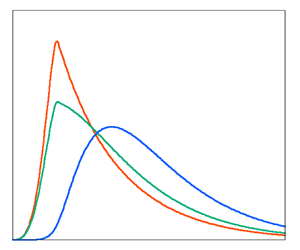
In three-dimensional (3-D) hydrodynamic turbulent flows, the scale-similarity law proposed by Kolmogorov (Reference Kolmogorov1941b) (which we will refer to as K41) has been foundational to turbulence theories. However, its validity or universality is still under discussion. A primitive element that can possibly break Kolmogorov's picture may be the breakage of mirror symmetry, where pseudoscalar quantities such as helicity possess finite values and play some physical roles. Helicity is defined by the volume average of the inner product of velocity and vorticity, and in addition to the kinetic energy, it is an inviscid invariant of the Navier–Stokes equations in three dimensions (Moffatt Reference Moffatt1969). Owing to the spontaneous appearance of helicity in turbulent flows subject to rotation (Marino et al. Reference Marino, Mininni, Rosenberg and Pouquet2013; Deusebio & Lindborg Reference Deusebio and Lindborg2014; Ranjan & Davidson Reference Ranjan and Davidson2014; Duarte et al. Reference Duarte, Wicht, Browning and Gastine2016; Inagaki & Hamba Reference Inagaki and Hamba2018), in such flows the effect of the breakage of mirror symmetry should be considered in small scales of Kolmogorov's locally isotropic turbulence. The existence of two different inviscid invariants is reminiscent of the two-dimensional (2-D) turbulence, in which energy and enstrophy are, respectively, conserved in an inviscid condition. In an analogy with the 2-D turbulence, Brissaud et al. (Reference Brissaud, Frisch, Leorat, Lesieur and Mazure1973) suggested several scale-similar structures in helical turbulence. One of these structures is the pure helicity cascade range, where the energy spectrum yields  $E(k) \propto (\varepsilon ^H)^{2/3} k^{-7/3}$. Another is the pure energy cascade range, where $E(k) \propto \varepsilon ^{2/3} k^{-5/3}$ with an inverse cascade. Notably, the helicity spectra in these ranges satisfy $E^H (k) \propto k E (k)$. Here, $E(k) [= \langle |\tilde {\boldsymbol {u}} (\boldsymbol {k})|^2 \rangle /(2{\rm \pi} k^2)]$ and $E^H (k) \{= \textrm {Re} [\langle \tilde {\boldsymbol {u}} (\boldsymbol {k}) \cdot \tilde {\boldsymbol {\omega }}^* (\boldsymbol {k}) \rangle ]/(4{\rm \pi} k^2)\}$ denote the energy and helicity spectra, $\tilde {\boldsymbol {u}}$ and $\tilde {\boldsymbol {\omega }}$ are the Fourier coefficients of velocity and vorticity, and where the superscript ${}^*$, $\langle \cdot \rangle$ and $k$ denote the complex conjugate, the statistical average involving the volume average and the wavenumber, respectively. Here $\varepsilon [= 2 \nu \int _0^\infty \mathrm {d}k\, k^2 E(k)]$ and $\varepsilon ^H [= 2 \nu \int _0^\infty \mathrm {d}k\, k^2 E^H(k)]$, respectively, denote the energy and helicity dissipation rates, where $\nu$ is the kinematic viscosity.
Recently, several studies numerically observed the pure helicity cascade or inverse energy cascade by attaining the maximally helical condition  $|E^H(k)| = 2k E(k)$, adopting an artificial cutoff of the nonlinear interaction of mixed-sign helical modes (Biferale, Musacchio & Toschi Reference Biferale, Musacchio and Toschi2012, Reference Biferale, Musacchio and Toschi2013; Sahoo, Bonaccorso & Biferale Reference Sahoo, Bonaccorso and Biferale2015), or employing a special forcing (Kessar et al. Reference Kessar, Plunian, Stepanov and Balarac2015; Stepanov et al. Reference Stepanov, Golbraikh, Frick and Shestakov2015; Plunian et al. Reference Plunian, Teimurazov, Stepanov and Verma2020). However, it is well known that the maximally helical condition $|E^H (k)| = 2k E(k)$ is not persistent in the dynamics of Navier–Stokes equations and that the turbulent field successively restores the mirror symmetry at small scales via the cascade process (Kraichnan Reference Kraichnan1973; Chen, Chen & Eyink Reference Chen, Chen and Eyink2003a). In contrast to the 2-D turbulence, where the energy and enstrophy spectra are connected by an equality, the helicity spectrum is bounded by an inequality, which is referred to as the realisability condition (Moffatt Reference Moffatt1978),
 \begin{equation} |E^H (k)| \le 2 k E (k). \end{equation}
Therefore, the helicity spectrum can be sufficiently small at different scales from the helicity injection scale. In the aforementioned studies on pure helicity cascade or inverse energy cascade, some modification of the nonlinear interaction or spacial forcing are essential elements for realising the maximally helical condition  $|E^H(k)| = 2k E(k)$ (Biferale et al. Reference Biferale, Musacchio and Toschi2012, Reference Biferale, Musacchio and Toschi2013; Kessar et al. Reference Kessar, Plunian, Stepanov and Balarac2015; Sahoo et al. Reference Sahoo, Bonaccorso and Biferale2015; Stepanov et al. Reference Stepanov, Golbraikh, Frick and Shestakov2015; Plunian et al. Reference Plunian, Teimurazov, Stepanov and Verma2020). In this regard, it would be beneficial to investigate the statistical similarity achieved by the pure nonlinearity of the Navier–Stokes equations.
In this study, we focus on the representative time scale to investigate the scale-similar structures of non-mirror-symmetric turbulence. The scale-similar spectra of energy and helicity are closely connected to the constant energy and helicity fluxes (Kraichnan Reference Kraichnan1971; Brissaud et al. Reference Brissaud, Frisch, Leorat, Lesieur and Mazure1973),
 \begin{equation} \varPi = \varepsilon \propto \omega_k k E(k),\quad \varPi^H = \varepsilon^H \propto \omega_k k E^H (k), \end{equation}
where  $\varPi$, $\varPi ^H$ and $\omega _k$ are the interscale energy and helicity fluxes and inverse of a representative time scale, respectively. Notably, the constant energy flux agrees with Kolmogorov's four-fifths law (Kolmogorov Reference Kolmogorov1941a; Frisch Reference Frisch1995). Similarly, the constant helicity flux agrees with the skew-symmetric third-order velocity correlation (Chkhetiani Reference Chkhetiani1996; L'vov, Podivilov & Procaccia Reference L'vov, Podivilov and Procaccia1997; Gomez, Politano & Pouquet Reference Gomez, Politano and Pouquet2000; Kurien Reference Kurien2003). By employing the conventional turbulence time scale $\omega _k \propto \varepsilon ^{1/3} k^{2/3}$, (1.2a,b) provides the conventional simultaneous or joint energy and helicity cascades range spectra (Brissaud et al. Reference Brissaud, Frisch, Leorat, Lesieur and Mazure1973),
 \begin{equation} E(k) = C_K \varepsilon^{2/3} k^{{-}5/3},\quad E^H(k) = C_H \varepsilon^H \varepsilon^{{-}1/3} k^{{-}5/3}, \end{equation}
where  $C_K$ and $C_H$ are constants. The spectra provided by (1.3a,b) are observed in the numerical simulations of homogeneous turbulence (Borue & Orszag Reference Borue and Orszag1997; Chen et al. Reference Chen, Chen and Eyink2003a,Reference Chen, Chen, Eyink and Holmb; Mininni, Alexakis & Pouquet Reference Mininni, Alexakis and Pouquet2006; Baerenzung et al. Reference Baerenzung, Politano, Ponty and Pouquet2008; Sahoo, De Pietro & Biferale Reference Sahoo, De Pietro and Biferale2017), an observation of an atmospheric boundary layer (Koprov et al. Reference Koprov, Koprov, Ponomarev and Chkhetiani2005), and a direct numerical simulation (DNS) of the Ekman boundary layer (Deusebio & Lindborg Reference Deusebio and Lindborg2014). It should be noted that Linkmann (Reference Linkmann2018) suggested the possibility of helicity altering the value of $C_K$, which poses a question on the universality of Kolmogorov's theory. In the magnetohydrodynamic turbulence case, the dominance of the time scale of a large-scale magnetic field supports the prediction that both the kinetic and magnetic energy spectra are proportional to $k^{-3/2}$ (Iroshnikov Reference Iroshnikov1964; Kraichnan Reference Kraichnan1965a; Yoshida & Arimitsu Reference Yoshida and Arimitsu2007). Even in the hydrodynamic case, Kurien, Taylor & Matsumoto (Reference Kurien, Taylor and Matsumoto2004a) suggested that the dominance of the helicity-related time scale $\omega _k^2 \propto |E^H (k)|k^2$ yields slightly shallow spectra,
 \begin{equation} E(k) \propto \varepsilon (\varepsilon^H)^{{-}1/3} k^{{-}4/3},\quad E^H(k) \propto (\varepsilon^H)^{2/3} k^{{-}4/3}. \end{equation}
They suggested that these spectra offer an interpretation of the bottleneck effect at small scales. Herbert et al. (Reference Herbert, Daviaud, Dubrulle, Nazarenko and Naso2012) observed another form of spectra that agree with the non-local effect of the large-scale shear-time scale in a von Kármán flow. Therefore, the representative time scale and the localness of the interscale interaction are the basis of scale-similar structures in turbulence.
The two-time velocity correlation and response function are relevant tools for obtaining a time scale without heuristic modelling. The response function was first introduced to turbulence by Kraichnan (Reference Kraichnan1959) in a statistical closure theory referred to as the direct interaction approximation (DIA). For a pioneering analysis of the non-mirror symmetric turbulence based on a closure theory, André & Lesieur (Reference André and Lesieur1977) investigated the effect of helicity via the eddy-damped quasi-normal Markovian (EDQNM) approximation. Recently, Briard & Gomez (Reference Briard and Gomez2017) discussed the detailed dynamics of helicity and its dissipation rate via EDQNM. However, it should be noted that the EDQNM phenomenologically employs the eddy-damping time scale  $\omega _k^2 \propto \int _0^k \mathrm {d}p \, p^2 E(p)$ (Lesieur Reference Lesieur2008). In contrast, the DIA dynamically determines the time scale via the two-time velocity correlation and response function. To obtain the closure equations consistent with the Kolmogorov spectrum, it is necessary to adopt the Lagrangian description (Kraichnan Reference Kraichnan1964, Reference Kraichnan1965b; Kaneda Reference Kaneda1981). In this study, we adopt the Lagrangian renormalised approximation (LRA) developed by Kaneda (Reference Kaneda1981). The LRA is analytically more convenient than the abridged Lagrangian history DIA (ALHDIA) developed by Kraichnan (Reference Kraichnan1965b). This study may be the first to investigate the effect of helicity on the scale-similar structures in homogeneous turbulence based on a self-consistent closure theory independent of any ad hoc adjusting parameters.
The rest of this paper is organised as follows. In § 2, we present some statistical properties of the Navier–Stokes equations and the closure equations of the LRA. In § 3, we discuss the scale-similar structures of LRA equations in the homogeneous isotropic and non-mirror-symmetric case. In this section, we also investigate the localness of the interscale interaction based on the closure equations. In § 4, we further discuss the properties of the closure equations and their relations with previous studies. Conclusions are provided in § 5.
2. Properties of the Navier–Stokes and closure equations
2.1. Basic equations for energy and helicity spectra
The Navier–Stokes equations for an incompressible fluid in Fourier space read
 \begin{equation} \left(\frac{\partial}{\partial t} + \nu k^2 \right) \tilde{u}_i (\boldsymbol{k},t) ={-} \mathrm{i}M_{ij\ell} (\boldsymbol{k}) \int \mathrm{d}^3\, p \int \mathrm{d}^3 q \,\delta (\boldsymbol{k} - \boldsymbol{p} - \boldsymbol{q}) \tilde{u}_j (\boldsymbol{p},t) \tilde{u}_\ell (\boldsymbol{q},t), \end{equation}
where  $\tilde {\boldsymbol {u}} (\boldsymbol {k},t)$ is the Fourier coefficient of the velocity field that satisfies the solenoidal condition $\boldsymbol {k} \cdot \tilde {\boldsymbol {u}} (\boldsymbol {k},t) = 0$, $M_{ij\ell } (\boldsymbol {k}) = [k_j P_{i\ell } (\boldsymbol {k}) + k_\ell P_{ij} (\boldsymbol {k})]/2$ and $P_{ij} (\boldsymbol {k}) = \delta _{ij} -k_i k_j/k^2$. The Fourier transformation of a variable $f(\boldsymbol {x},t)$ and its inverse transformation are defined by
 \begin{equation} f (\boldsymbol{x},t) = \int \mathrm{d}^3 k \, \tilde{f} (\boldsymbol{k},t) \,\mathrm{e}^{\mathrm{i} \boldsymbol{k} \cdot \boldsymbol{x}},\quad \tilde{f} (\boldsymbol{k},t) = \frac{1}{(2{\rm \pi})^3} \int \mathrm{d}^3 x \, f (\boldsymbol{x},t)\, \mathrm{e}^{-\mathrm{i} \boldsymbol{k} \cdot \boldsymbol{x}}. \end{equation}
The equations for energy and helicity spectra,  $E (k,t)$ and $E^H (k,t)$, yield
 \begin{gather} \left(\frac{\partial}{\partial t} + 2 \nu k^2 \right) E (k,t) = \frac{1}{2} \int _0^\infty \mathrm{d} p\, \int_0^\infty \mathrm{d}q \, S (k,p,q,t), \end{gather}
 \begin{gather}\left(\frac{\partial}{\partial t} + 2 \nu k^2 \right) E^H (k,t) = \frac{1}{2} \int _0^\infty \mathrm{d} p \,\int_0^\infty \mathrm{d}q \, S^H (k,p,q,t), \end{gather}
where
 \begin{gather} S (k,p,q,t) ={-} 16{\rm \pi}^2 kpq \varDelta_{kpq} M_{ij\ell} (\boldsymbol{k}) \textrm{Im} [\langle \tilde{u}_i (\boldsymbol{k},t) \tilde{u}_j (-\boldsymbol{p},t) \tilde{u}_\ell (-\boldsymbol{q},t) \rangle], \end{gather}
 \begin{gather}S^H (k,p,q,t) ={-} 16{\rm \pi}^2 kpq \varDelta_{kpq} \left(\epsilon_{ijm} k_\ell + \epsilon_{i\ell m} k_j\right) k_m \textrm{Re} [ \langle \tilde{u}_i (\boldsymbol{k},t) \tilde{u}_j (-\boldsymbol{p},t) \tilde{u}_\ell (-\boldsymbol{q},t) \rangle], \end{gather}
and  $\varDelta _{kpq}$ is unity only when $k$,
$k$,  $p$ and $q$ can form the sides of a triangle. The conservation of energy and helicity are guaranteed by the detailed balance (see e.g. Waleffe Reference Waleffe1992)
 \begin{gather} S (k,p,q,t) + S (p,q,k,t) + S (q,k,p,t) = 0, \end{gather}
 \begin{gather}S^H (k,p,q,t) + S^H (p,q,k,t) + S^H (q,k,p,t) = 0. \end{gather}
Therefore, we have
 \begin{equation} \int _0^\infty \mathrm{d}k \int _0^\infty \mathrm{d}p \int_0^\infty \mathrm{d}q \, S (k,p,q,t) = 0,\quad \int _0^\infty \mathrm{d}k \int _0^\infty \mathrm{d}p \int_0^\infty \mathrm{d}q \, S^H (k,p,q,t) = 0. \end{equation}
Interscale energy flux  $\varPi (k,t)$ and helicity flux $\varPi ^H (k,t)$ are defined by
 \begin{align} \varPi (k,t) &= \tfrac{1}{2} \int_k^\infty \mathrm{d} k' \int _0^\infty \mathrm{d} p' \int_0^\infty \mathrm{d} q' S (k',p',q',t) \nonumber\\ &={-} \tfrac{1}{2} \int_0^k \mathrm{d} k' \int _0^\infty \mathrm{d} p' \int_0^\infty \mathrm{d}q' \,S (k',p',q',t), \end{align}
 \begin{align} \varPi^H (k,t) &= \tfrac{1}{2} \int_k^\infty \mathrm{d} k' \int _0^\infty \mathrm{d} p' \int_0^\infty \mathrm{d}q' \, S^H (k',p',q',t) \nonumber\\ &={-} \tfrac{1}{2} \int_0^k \mathrm{d} k' \int _0^\infty \mathrm{d} p' \int_0^\infty \mathrm{d}q' \,S^H (k',p',q',t), \end{align}
where we utilise (2.9a,b).
Considering the maximally helical or homochiral condition,
 \begin{equation} E^H (k,t) = 2k E(k,t). \end{equation}
This condition holds for the Beltrami velocity field, which is defined by  $\mathrm {i} \boldsymbol {k} \times \tilde {\boldsymbol {u}} (\boldsymbol {k},t) = k \tilde {\boldsymbol {u}} (\boldsymbol {k},t)$. For the Beltrami velocity field, $S^H(k,p,q,t)$ satisfies
 \begin{equation} S^H(k,p,q,t) = 2 k S(k,p,q,t), \end{equation}
which denotes a maximally helical condition for the third moment. Using (2.13), the detailed balance for helicity (2.8) yields
 \begin{equation} k S (k,p,q,t) + p S (p,q,k,t) + q S (q,k,p,t) = 0. \end{equation}
Similarly, the Navier–Stokes equations in two dimensions provide the equation  $k^2 S (k,p,q,t) + p^2 S (p,q,k,t) + q^2 S (q,k,p,t) = 0$, which guarantees the conservation of enstrophy. Waleffe (Reference Waleffe1992) analysed the statistical properties of the Navier–Stokes equations by employing the scale-similar structure and the two detailed balance (2.7) and (2.14), which verified that the nonlinear interaction of the velocity fields comprising the same sign helical modes can trigger an inverse transfer of energy. However, it is demonstrated that the turbulent field successively restores the mirror symmetry at small scales via the cascade process (Kraichnan Reference Kraichnan1973; Chen et al. Reference Chen, Chen and Eyink2003a). Hence, the maximally helical condition (2.12) is not persistent in the dynamics of the Navier–Stokes equations. The relationship between this tendency and the property of the closure equations is discussed in Appendix A.
2.2. Properties of closure equations
In this study, we adopt the LRA (Kaneda Reference Kaneda1981) as a closure approximation. For details on the closure, see Kaneda (Reference Kaneda1981, Reference Kaneda2007). A unique feature of LRA is in introducing a mapping function from Eulerian to Lagrangian velocities,
 \begin{equation} \boldsymbol{v} (\boldsymbol{x}, s\,|\, t) = \int \mathrm{d}^3x' \,\psi (\boldsymbol{x}',t\,|\, \boldsymbol{x},s) \boldsymbol{u} (\boldsymbol{x}', t), \end{equation}
where  $\boldsymbol {v} (\boldsymbol {x}, s\,|\, t)$ denotes the Lagrangian velocity and $\psi (\boldsymbol {x}',t\,|\, \boldsymbol {x},s)$ denotes the Lagrangian position function that obeys
 \begin{equation} \frac{\partial}{\partial t} \psi (\boldsymbol{x}, t\,|\, \boldsymbol{x}', s) + u_i (\boldsymbol{x},t) \frac{\partial}{\partial x_i} \psi (\boldsymbol{x}, t\,|\, \boldsymbol{x}', s) = 0, \end{equation}
with  $\psi (\boldsymbol {x},s\,|\, \boldsymbol {x}',s) = \delta (\boldsymbol {x} - \boldsymbol {x}')$. Namely, $\boldsymbol {v} (\boldsymbol {x}, s\,|\, t)$ denotes the velocity of the fluid element at time $t$ which was at $\boldsymbol {x}$ at time $s$. Notably, the Lagrangian velocity satisfies
 \begin{equation} \boldsymbol{v} (\boldsymbol{x}, s\,|\, s) = \boldsymbol{u} (\boldsymbol{x}, s). \end{equation}
For the representative variables, the LRA adopts the Lagrangian two-time velocity correlation  $Q_{ij} (\boldsymbol {k}, t,s)$ and the mean Lagrangian response function $G_{ij} (\boldsymbol {k},t,s)$. They are defined by
 \begin{gather} Q_{ij} (\boldsymbol{k}, t, s) \delta (\boldsymbol{k} + \boldsymbol{k}') = P_{ia} (\boldsymbol{k}) \left\langle \tilde{v}_a (\boldsymbol{k}, s\,|\,t) \tilde{u}_j (\boldsymbol{k}',s) \right \rangle, \end{gather}
 \begin{gather}G_{ij} (\boldsymbol{k}, t, s) \delta (\boldsymbol{k} - \boldsymbol{k}') = P_{ia} (\boldsymbol{k}) P_{jb} (\boldsymbol{k}) \left\langle \frac{\delta \tilde{v}_a (\boldsymbol{k}, s\,|\, t)}{\delta \tilde{f}_b (\boldsymbol{k}',s)} \right \rangle, \end{gather}
where  $\delta \tilde {\boldsymbol {f}} (\boldsymbol {k},t)$ denotes an infinitesimal forcing driving an infinitesimal perturbation in the Eulerian velocity field $\delta \tilde {\boldsymbol {u}} (\boldsymbol {k},t)$; $\delta \tilde {\boldsymbol {u}} (\boldsymbol {k},t)$ obeys
 \begin{align} \left(\frac{\partial}{\partial t} + \nu k^2\right) \delta \tilde{u}_i (k,t) &={-} 2 \mathrm{i} M_{ij\ell} (\boldsymbol{k}) \int \mathrm{d}^3p \int \mathrm{d}^3 q \, \delta (\boldsymbol{k} - \boldsymbol{p} - \boldsymbol{q})\tilde{u}_j (\boldsymbol{p},t) \delta \tilde{u}_\ell (\boldsymbol{q},t) \nonumber\\ &\quad + P_{ij} (\boldsymbol{k}) \delta \tilde{f}_j (\boldsymbol{k},t). \end{align}
The initial condition for the response function  $G_{ij} (\boldsymbol {k},s,s)$ is determined as follows. Based on (2.17) and (2.19), we have
 \begin{equation} G_{ij} (\boldsymbol{k}, s, s) \delta (\boldsymbol{k} - \boldsymbol{k}') = P_{ia} (\boldsymbol{k}) P_{jb} (\boldsymbol{k}) \left\langle \tilde{G}^\mathrm{E}_{ab} (\boldsymbol{k},s\,|\,\boldsymbol{k}',s) \right \rangle, \end{equation}
where
 \begin{equation} \tilde{G}^\mathrm{E}_{ij} (\boldsymbol{k},t\,|\,\boldsymbol{k}',s) = \frac{\delta \tilde{u}_i (\boldsymbol{k}, t)}{\delta \tilde{f}_j (\boldsymbol{k}',s)} \end{equation}
and thus,
 \begin{equation} \delta \tilde{u}_i (\boldsymbol{k}, t) = \int_{t_0}^t \mathrm{d}s \int \mathrm{d}^3k'\, \tilde{G}^\mathrm{E}_{ij} (\boldsymbol{k},t\,|\,\boldsymbol{k}',s) \delta \tilde{f}_j (\boldsymbol{k}',s), \end{equation}
where  $t_0$ is the initial time. $\tilde {G}^\mathrm {E}_{ij} (\boldsymbol {k},t\,|\,\boldsymbol {k}',s)$ denotes the Eulerian response function that obeys
 \begin{align} \left(\frac{\partial}{\partial t} + \nu k^2 \right) \tilde{G}^\mathrm{E}_{ij} (\boldsymbol{k},t\,|\,\boldsymbol{k}',s) &={-} 2 \mathrm{i} M_{i\ell m} (\boldsymbol{k}) \int \mathrm{d}^3 p \int \mathrm{d}^3 q \, \delta (\boldsymbol{k} - \boldsymbol{p} - \boldsymbol{q}) \nonumber\\ &\quad \times \tilde{u}_\ell (\boldsymbol{p},t) \tilde{G}^\mathrm{E}_{mj} (\boldsymbol{q},t\,|\,\boldsymbol{k}',s). \end{align}
The time derivative of the right-hand side of (2.23) must correspond to (2.20), which requires
 \begin{equation} \tilde{G}^\mathrm{E}_{ij} (\boldsymbol{k},t\,|\,\boldsymbol{k}',t) = P_{ij} (\boldsymbol{k}) \delta (\boldsymbol{k} - \boldsymbol{k}'). \end{equation}
Accordingly, the initial condition for the mean Lagrangian response function yields
 \begin{equation} G_{ij} (\boldsymbol{k}, s, s) = P_{ij} (\boldsymbol{k}). \end{equation}
Notably, (2.21) should hold even when we adopt another type of response function as the representative. Hence, the initial condition (2.26) is general for the closure theories employing the response function.
For the LRA, the closure equations yield (Kaneda Reference Kaneda1981)
 \begin{gather} \left(\frac{\partial}{\partial t} + 2\nu k^2 \right) Q_{ij} (\boldsymbol{k}, t,t) = T_{ij} (\boldsymbol{k},t) + T_{ji} (-\boldsymbol{k},t), \end{gather}
 \begin{gather}\left(\frac{\partial}{\partial t} + \nu k^2 \right) Q_{ij} (\boldsymbol{k}, t,s) ={-} \eta_{ia} (\boldsymbol{k},t,s) Q_{aj} (\boldsymbol{k}, t,s) \quad (t > s), \end{gather}
 \begin{gather}\left(\frac{\partial}{\partial t} + \nu k^2 \right) G_{ij} (\boldsymbol{k}, t,s) ={-} \eta_{ia} (\boldsymbol{k},t,s) G_{aj} (\boldsymbol{k}, t,s) \quad (t > s), \end{gather}
where
 \begin{align} T_{ij} (\boldsymbol{k},t) &= M_{i\ell m} (\boldsymbol{k}) \int \mathrm{d}^3 p \int \mathrm{d}^3 q \, \delta(\boldsymbol{k}- \boldsymbol{p} - \boldsymbol{q}) \int_{t_0}^t \mathrm{d} s \nonumber\\ &\quad \times \left[ - 4M_{abc} (\boldsymbol{p}) G_{ma} (\boldsymbol{p},t,s) Q_{\ell b} (\boldsymbol{q},t,s) Q_{jc} (-\boldsymbol{k},t,s) \right. \nonumber\\ &\quad + \left. 2M_{abc} (\boldsymbol{k}) G_{ja} (-\boldsymbol{k},t,s) Q_{mc} (\boldsymbol{p},t,s) Q_{\ell b} (\boldsymbol{q},t,s)\right], \end{align}
 \begin{align} \eta_{ij} (\boldsymbol{k},t,s) &= 2 \int \mathrm{d}^3 p \int \mathrm{d}^3 q \, \delta(\boldsymbol{k} - \boldsymbol{p} - \boldsymbol{q}) P_{ib} (\boldsymbol{k}) \frac{q_j q_b q_\ell q_m}{q^2} \int_{s}^t \mathrm{d} s' \,Q_{\ell m} (-\boldsymbol{p},t,s'). \end{align}
For a homogeneous isotropic and non-mirror symmetric case, second-order tensor variables read
 \begin{gather} Q_{ij} (\boldsymbol{k},t,s) = \frac{1}{2} P_{ij} (\boldsymbol{k}) Q (k,t,s) - \frac{\mathrm{i}}{2} \epsilon_{ij\ell} \frac{k_\ell}{k^2} Q^H (k,t,s), \end{gather}
 \begin{gather}G_{ij} (\boldsymbol{k},t,s) = P_{ij} (\boldsymbol{k}) G (k,t,s) - \mathrm{i} \epsilon_{ij\ell} \frac{k_\ell}{k} G^H (k,t,s), \end{gather}
where  $Q(k,t,s)$ and $Q^H(k,t,s)$ are related to the energy and helicity spectra, respectively, and are expressed as
 \begin{equation} Q(k,t,t) = \frac{E(k,t)}{2{\rm \pi} k^2},\quad Q^H(k,t,t) = \frac{E^H(k,t)}{4{\rm \pi} k^2}, \end{equation}
where  $Q(k,t,t)$ and $Q^H (k,t,t)$ denote the spectral densities of energy and helicity, respectively.
The trace parts of (2.27)–(2.29) yield the equations for  $Q(k,t,t)$, $Q(k,t,s)$ and $G(k,t,s)$, respectively. Meanwhile, multiplying (2.27)–(2.29) by $\mathrm {i} \epsilon _{ijn} k_n$ yields the equations for $Q^H(k,t,t)$, $Q^H(k,t,s)$ and $G^H(k,t,s)$, respectively. The resulting equations yield
 \begin{align} & \left(\frac{\partial}{\partial t} + 2\nu k^2 \right) Q (k,t,t) = 2 {\rm \pi}\int_0^\infty \mathrm{d}p \int_0^\infty \mathrm{d}q \,\varDelta_{kpq} \int_{t_0}^t \mathrm{d}s \nonumber\\ &\quad \times\left\{kpq b_{kpq} \left[ G(k,t,s) Q (p,t,s) - G(p,t,s) Q (k,t,s)\right] Q (q,t,s) \vphantom{\left[ \frac{p^2}{k} G^H (k,t,s) Q (p,t,s) - p G^H (p,t,s) Q (k,t,s) \right] }\right. \nonumber\\ &\quad -\frac{pq}{k} c_{kpq} \left[ G(k,t,s) Q^H (p,t,s) - G(p,t,s) Q^H (k,t,s) \right] Q^H (q,t,s) \nonumber\\ &\quad + \frac{pq}{k} \left[ b_{kpq} k G^H (k,t,s) Q^H (p,t,s) - c_{kpq} p G^H (p,t,s) Q^H (k,t,s) \right] Q (q,t,s) \nonumber\\ &\quad - \left. \frac{pq}{k} c_{kpq} \left[ \frac{p^2}{k} G^H (k,t,s) Q (p,t,s) - p G^H (p,t,s) Q (k,t,s) \right] Q^H (q,t,s) \right\}, \end{align}
 \begin{align} & \left( \frac{\partial}{\partial t} + 2\nu k^2 \right) Q^H (k,t,t) = 2 {\rm \pi}\int_0^\infty \mathrm{d}p \int_0^\infty \mathrm{d}q \,\varDelta_{kpq} \int_{t_0}^t \mathrm{d}s \nonumber\\ &\quad \times \left\{ kpq b_{kpq} \left[ G(k,t,s) Q^H (p,t,s) - G(p,t,s) Q^H (k,t,s) \right] Q (q,t,s) \vphantom{\left[ \frac{p^2}{k} G^H (k,t,s) Q (p,t,s) - p G^H (p,t,s) Q (k,t,s) \right] } \right. \nonumber\\ &\quad - \frac{pq}{k} c_{kpq} \left[ p^2 G(k,t,s) Q (p,t,s) - k^2G(p,t,s) Q (k,t,s) \right] Q^H (q,t,s) \nonumber\\ &\quad + kpq \left[ b_{kpq} k G^H (k,t,s) Q (p,t,s) - c_{kpq} p G^H (p,t,s) Q (k,t,s) \right] Q (q,t,s) \nonumber\\ &\quad - \left.\vphantom{\left[ \frac{p^2}{k} G^H (k,t,s) Q (p,t,s) - p G^H (p,t,s) Q (k,t,s) \right] } \frac{pq}{k} c_{kpq} \left[ k G^H (k,t,s) Q^H (p,t,s) - p G^H (p,t,s) Q^H (k,t,s) \right] Q^H (q,t,s) \right\}, \end{align}
 \begin{gather} \left[ \frac{\partial}{\partial t} + \nu k^2 + \eta(k,t,s) \right] Q (k, t,s) = 0 \quad (t > s), \end{gather}
 \begin{gather}\left[ \frac{\partial}{\partial t} + \nu k^2 + \eta(k,t,s) \right] Q^H (k, t,s) = 0\quad (t > s), \end{gather}
 \begin{gather}\left[ \frac{\partial}{\partial t} + \nu k^2 + \eta(k,t,s) \right] G (k, t,s) = 0 \quad (t > s), \end{gather}
 \begin{gather}\left[ \frac{\partial}{\partial t} + \nu k^2 + \eta(k,t,s) \right] G^H (k, t,s) = 0\quad (t > s), \end{gather}
where
 \begin{gather} \eta (k,t,s) = k \int_0^\infty \mathrm{d}q \ q^3 J \left(\frac{q}{k} \right) \int_s^t \mathrm{d}s'\, Q (q,t,s'), \end{gather}
 \begin{gather}J(x) = \frac{\rm \pi}{2a^4} \left[ (a^2-1)^2 \ln \left( \frac{1+a}{|1-a|} \right) - 2a + \frac{10}{3} a^3 \right], \quad a = \frac{2x}{1+x^2} \end{gather}
and
 \begin{equation} \left.\begin{gathered} b_{kpq} = \frac{p}{k} (xy + z^3), \quad c_{kpq} = \frac{k}{q} z (x+yz) = \frac{k}{p} z (1-y^2), \nonumber \\ x = \frac{p^2+q^2-k^2}{2pq}, \quad y = \frac{q^2+k^2-p^2}{2qk}, \quad z = \frac{k^2+p^2-q^2}{2kp}. \end{gathered}\right\} \end{equation}
Details on the calculations are provided in Appendix B. Hence, for the closure equations,  $S(k,p,q,t)$ and $S^H (k,p,q,t)$ in (2.3)–(2.6) read
 \begin{align} & S (k,p,q,t) = 4 {\rm \pi}^2 \varDelta_{kpq} \int_{t_0}^t \mathrm{d}s \, kpq \nonumber\\ &\quad \times \left\{ k^2 \left[ (b_{kpq} + b_{kqp}) G(k,t,s) Q (p,t,s) Q (q,t,s) \right. \vphantom{\frac{q^2}{k}} \right. \nonumber\\ &\quad - \left. b_{kpq} G(p,t,s) Q (k,t,s) Q (q,t,s) - b_{kqp} G(q,t,s) Q (k,t,s) Q (p,t,s)\right] \nonumber\\ &\quad - \left[ (c_{kpq} + c_{kqp}) G(k,t,s) Q^H (p,t,s) Q^H (q,t,s) \right. \nonumber\\ &\quad - \left. c_{kpq} G(p,t,s) Q^H (k,t,s) Q^H (q,t,s) - c_{kqp} G(q,t,s) Q^H (k,t,s) Q^H(p,t,s)\right] \nonumber\\ &\quad + k \left[ b_{kpq} G^H (k,t,s) Q^H (p,t,s) Q (q,t,s) + b_{kqp} G^H (k,t,s) Q (p,t,s) Q^H (q,t,s) \vphantom{\left[ \frac{p}{k} G^H (k,t,s) Q (p,t,s) - p G^H (p,t,s) Q (k,t,s) \right]}\right. \nonumber\\ &\quad - \left. \frac{p}{k} c_{kpq} G^H (p,t,s) Q^H (k,t,s) Q (q,t,s) - \frac{q}{k} c_{kqp} G^H (q,t,s) Q^H (k,t,s) Q (p,t,s) \right] \nonumber\\ &\quad - k \left[ \frac{p^2}{k^2} c_{kpq} G^H (k,t,s) Q (p,t,s) Q^H (q,t,s) + \frac{q^2}{k^2} c_{kqp} G^H (k,t,s) Q^H (p,t,s) Q (q,t,s) \right. \nonumber\\ &\quad - \frac{p}{k} c_{kpq} G^H (p,t,s) Q (k,t,s) Q^H (q,t,s) \nonumber\\ &\quad - \left.\left. \frac{q}{k} c_{kqp} G^H (q,t,s) Q (k,t,s) Q^H (p,t,s) \vphantom{\frac{q^2}{k}}\right] \right\}, \end{align}
 \begin{align} & S^H (k,p,q,t) = 8 {\rm \pi}^2 \varDelta_{kpq} \int_{t_0}^t \mathrm{d}s \, kpq \nonumber\\ &\quad \times \left\{ k^2 \left[ b_{kpq} G(k,t,s) Q^H (p,t,s) Q (q,t,s) + b_{kqp} G(k,t,s) Q (p,t,s) Q^H (q,t,s) \right. \vphantom{\left[ \frac{p^2}{k} G^H (k,t,s) Q (p,t,s) - p G^H (p,t,s) Q (k,t,s) \right] }\right. \nonumber\\ &\quad - \left. b_{kpq} G(p,t,s) Q^H (k,t,s) Q (q,t,s) - b_{kqp} G(q,t,s) Q^H (k,t,s) Q (p,t,s) \right] \nonumber\\ &\quad - k^2 \left[ \frac{p^2}{k^2} c_{kpq} G (k,t,s) Q (p,t,s) Q^H (q,t,s) + \frac{q^2}{k^2} c_{kqp} G (k,t,s) Q^H (p,t,s) Q (q,t,s) \right. \nonumber\\ &\quad - \left.\vphantom{\left[ \frac{p^2}{k} G^H (k,t,s) Q (p,t,s) - p G^H (p,t,s) Q (k,t,s)\right]} c_{kpq} G(p,t,s) Q (k,t,s) Q^H (q,t,s) - c_{kqp} G(q,t,s) Q (k,t,s) Q^H (p,t,s) \right] \nonumber\\ &\quad + k^3 \left[ (b_{kpq} + b_{kqp}) G^H (k,t,s) Q (p,t,s) Q (q,t,s) \vphantom{\left[ \frac{p}{k} G^H (k,t,s) Q (p,t,s) - p G^H (p,t,s) Q (k,t,s) \right] }\right. \nonumber\\ &\quad - \left. \frac{p}{k} c_{kpq} G^H (p,t,s) Q (k,t,s) Q (q,t,s) - \frac{q}{k} c_{kqp} G^H (q,t,s) Q (k,t,s) Q (p,t,s) \right] \nonumber\\ &\quad - k \left[ (c_{kpq} + c_{kqp}) G^H (k,t,s) Q^H (p,t,s) Q^H (q,t,s) \vphantom{\left[ \frac{p}{k} G^H (k,t,s) Q (p,t,s) - p G^H (p,t,s) Q (k,t,s) \right]}\right. \nonumber\\ &\quad - \frac{p}{k} c_{kpq} G^H (p,t,s) Q^H (k,t,s) Q^H (q,t,s) \nonumber\\ &\quad - \left.\vphantom{\left[ \frac{p^2}{k} G^H (k,t,s) Q (p,t,s) - p G^H (p,t,s) Q (k,t,s) \right] } \left. \frac{q}{k} c_{kqp} G^H (q,t,s) Q^H (k,t,s) Q^H (p,t,s) \right]\right\}, \end{align}
where we adopt the symmetry in  $p$ and $q$. Equations (2.44) and (2.45) satisfy the detailed balance provided by (2.7) and (2.8), which is presented in Appendix C.
It should be noted that these triple correlations in the closure do not satisfy the maximally helical condition for the third moment given by (2.13) even if the energy and helicity spectra are maximally helical; namely, the closure yields
 \begin{equation} S^H (k,p,q,t) \neq 2k S (k,p,q,t), \end{equation}
even if  $E^H (k,t) = 2k E(k,t)$ at the time $t$ (see also Appendix A). Although this result is not unique to the LRA, it holds for other closures based on the two-point velocity correlations such as the EDQNM, DIA and ALHDIA. The fact that the closure equations are inconsistent with the maximally helical condition is physically plausible. We define the relative helicity as
 \begin{equation} \rho^H (k,t) = \frac{E^H(k,t)}{2k E(k,t)}. \end{equation}
The relative helicity must be bounded via the realisability condition (1.1), namely
 \begin{equation} |\rho^H (k,t)| \le 1. \end{equation}
For homogeneous turbulence, it is well known that the relative helicity  $\rho ^H(k,t)$ decreases even when it starts from the maximally helical condition $\rho ^H(k,t_0)=1$ (Morinishi, Nakabayashi & Ren Reference Morinishi, Nakabayashi and Ren2001). The closure equations follow this property. Actually, the EDQNM predicts the same tendency (André & Lesieur Reference André and Lesieur1977; Briard & Gomez Reference Briard and Gomez2017). Although some special forcing may realise the maximally helical spectra (Kessar et al. Reference Kessar, Plunian, Stepanov and Balarac2015; Stepanov et al. Reference Stepanov, Golbraikh, Frick and Shestakov2015; Plunian et al. Reference Plunian, Teimurazov, Stepanov and Verma2020), it is beyond the scope of this study because we focus on the scale-similar structures achieved by the nonlinearity of the Navier–Stokes equations. Considering this point, the property (2.13) derived from the Navier–Stokes equations with the Beltrami velocity field possibly holds only for the subensemble satisfying $\mathrm {i} \boldsymbol {k} \times \tilde {\boldsymbol {u}} (\boldsymbol {k},t) = k \tilde {\boldsymbol {u}} (\boldsymbol {k},t)$.
For the LRA,  $Q(k,t,s)$, $Q^H (k,t,s)$, $G (k,t,s)$ and $G^H (k,t,s)$ obey the same equation as presented in (2.37)–(2.40). The initial condition for the response function (2.26) yields $G(k,s,s) = 1$ and $G^H (k,s,s) = 0$. The latter with (2.40) yields $G^H (k,t,s) = 0$. Therefore, the non-mirror-symmetric part of the response function must disappear for the LRA. Using the mirror-symmetric part of the response function $G (k,t,s)$, the two-time velocity correlations are reduced to
 \begin{gather} Q(k,t,s) = G(k,t,s) Q(k,s,s) \quad (t \ge s), \end{gather}
 \begin{gather}Q^H (k,t,s) = G(k,t,s) Q^H (k,s,s) \quad (t \ge s), \end{gather}
which represent the fluctuation-dissipation theorem (FDT) (Marconi et al. Reference Marconi, Puglisi, Rondoni and Vulpiani2008; Matsumoto et al. Reference Matsumoto, Otsuki, Ooshida and Goto2021). It is a feature of LRA that the FDT holds. It should be noted that helicity does not directly influence the response function because  $\eta (k,t,s)$, given by (2.41), is solely determined by the mirror-symmetric part of the velocity correlation. Therefore, the effect of the breakage of mirror symmetry disappears from the response function (2.39). Similarly, Kaneda & Gotoh (Reference Kaneda and Gotoh1991) and Rubinstein & Zhou (Reference Rubinstein and Zhou1999) demonstrated that helicity does not affect the Lagrangian two-time velocity correlation. Therefore, we infer that the breakage of mirror symmetry does not affect both the response function and Lagrangian two-time velocity correlation for the LRA.
Using (2.49), (2.50) and  $G^H (k,t,s) = 0$, the equations for the spectral densities of energy and helicity (2.35) and (2.36) yield
 \begin{align} \left( \frac{\partial}{\partial t} + 2\nu k^2 \right) Q (k,t,t) & = 2 {\rm \pi}\int_0^\infty \mathrm{d}p \int_0^\infty \mathrm{d}q \varDelta_{kpq} \int_{t_0}^t \mathrm{d}s \, G(k,t,s) G(p,t,s) G(q,t,s) \nonumber\\ & \quad \times \left\{ kpq b_{kpq} \left[ Q (p,s,s) - Q (k,s,s) \right] Q (q,s,s) \vphantom{\frac{pq}{k}}\right. \nonumber\\ &\quad - \left. \frac{pq}{k} c_{kpq} \left[ Q^H (p,s,s) - Q^H (k,s,s) \right] Q^H (q,s,s)\right\}, \end{align}
 \begin{align} \left(\frac{\partial}{\partial t} + 2\nu k^2 \right) Q^H (k,t,t) &= 2 {\rm \pi}\int_0^\infty \mathrm{d}p \int_0^\infty \mathrm{d}q \,\varDelta_{kpq} \int_{t_0}^t \mathrm{d}s \, G(k,t,s) G(p,t,s) G(q,t,s) \nonumber\\ &\quad \times \left\{ kpq b_{kpq} \left[ Q^H (p,s,s) - Q^H (k,s,s) \right] Q (q,s,s) \vphantom{\frac{pq}{k} }\right. \nonumber\\ &\quad - \left. \frac{pq}{k} c_{kpq} \left[ p^2 Q (p,s,s) - k^2 Q (k,s,s) \right] Q^H (q,s,s)\right\}. \end{align}
They possess the same form as the EDQNM except for the expression of the relaxation time. The LRA dynamically determines the relaxation time using the response function  $G(k,t,s)$, whereas the EDQNM phenomenologically employs the eddy damping time scale (Orszag Reference Orszag1970; Lesieur Reference Lesieur2008).
The numerical simulation of the integro-differential equations provided by (2.39), (2.51) and (2.52) is a primitive approach to investigating the physical properties of the closure equations. However, the LRA involves time integration in the nonlinear interaction term of energy and helicity (2.51) and (2.52). Therefore, we have to perform the triple integration of  $p$,
$p$,  $q$ and $s$ for the numerical simulation of LRA, whereas the EDQNM reduces this into the double integral of $p$ and $q$. Consequently, the computation time of LRA increases proportionally to $N_t$ compared with that of EDQNM, where $N_t$ denotes the number of the numerical time step. Therefore, the long-time integration of the high Reynolds number simulation of LRA remains a challenge. For the practical simulations of LRA, reductions such as Markovianisation (Gotoh, Kaneda & Bekki Reference Gotoh, Kaneda and Bekki1988) and the single-time expression of the response function with a short time expansion (Kitamura Reference Kitamura2020) may be effective. It is noteworthy that numerical simulations of closure equations are beneficial when we explore the behaviour of turbulence around the integral and viscous scales. Probably, differences between EDQNM type models and LRA are even more important around these scales than in the inertial range. However, in this study, we focus on the scale similarity of the LRA equations as a first step in understanding the physical properties of the theoretical closure approximation of turbulence in a non-mirror symmetric case. In future work, we will perform the numerical simulations of LRA to explore the behaviour of turbulence outside the similarity range. As will be discussed later, the scale similarity for the simultaneous energy and helicity cascades requires significantly more extensive scale separation than the mirror-symmetric case. In this study, we assume long range similarity scalings and investigate the analytical properties of the LRA for the non-mirror-symmetric case, instead of numerically solving the closure equations.
3. Scale-similar analysis
3.1. Scale similarity assumptions
Here, we assume the extended scale-similar spectra for energy and helicity (Golbraikh & Moiseev Reference Golbraikh and Moiseev2002; Golbraikh Reference Golbraikh2006; Kessar et al. Reference Kessar, Plunian, Stepanov and Balarac2015),
 \begin{equation} E(k) = C_K^{(n)} \varepsilon^{7/3-n} (\varepsilon^H)^{{-}5/3+n} k^{{-}n}, \quad E^H(k) = C_H^{(m)} \varepsilon^{4/3-m} (\varepsilon^H)^{{-}2/3+m} k^{{-}m}, \end{equation}
where  $C_K^{(n)}$ and $C_H^{(m)}$ are constants expected to be universal. In addition, the scale-similar time scale reads
 \begin{equation} \omega_k^{{-}1} = \varepsilon^{1/3-\ell} (\varepsilon^H)^{{-}2/3+\ell} k^{-\ell}. \end{equation}
Considering the simultaneous cascades of energy and helicity, an additional internal wavenumber or length scale exists (Moiseev & Chkhetiani Reference Moiseev and Chkhetiani1996):
 \begin{equation} k^H = \varepsilon^H/ \varepsilon. \end{equation}
According to K41 (Kolmogorov Reference Kolmogorov1941b), we assume that the field is approximately statistically steady in the inertial range. In such a case, the spectra and response function are reduced to
 \begin{equation} Q(k,t,t) = Q(k), \quad Q^H(k,t,t) = Q^H(k),\quad G(k,t,s) = G(k,t-s) = G(\omega_k(t-s)). \end{equation}
One may consider that the scale-similar spectra (3.1a,b) should have the lower and upper bounds  $k_{lower}$ and $k_{upper}$, and the response function equation and energy and helicity fluxes are affected from outside the scale-similar range such as the energy-containing and viscous ranges. In the following analyses, the wavenumber variables of integration are normalised by the wavenumber $k$ that lies in the similarity range. In such a case, the integral region accompanied by the similarity laws (3.1a,b), (3.2) and (3.4a–c) extends to the whole wavenumber range in the limit $k_{lower}/k \to 0$ and $k_{upper}/k \to \infty$. If the contributions from outside the similarity range vanish in the limit, one can justify this similarity analysis that the response function equation and energy and helicity fluxes are determined solely by the contributions from the similarity range. Details for the condition for the contributions from outside the similarity range to vanish are given in the supplementary material available at https://doi.org/10.1017/jfm.2021.708. The following scale-similarity analysis considers the situation that the scale-similar spectra extend to a sufficiently wide range that allows for the assumption $k_{lower}/k \ll 1$ and $k_{upper}/k \gg 1$. Besides, if distant interactions such expressed by the contributions from the wavenumber $\sim k_{lower}$ or $k_{upper}$ are not negligible, the wavenumber integral can diverge and this similarity analysis would lose its meaning. We will discuss the conditions for these integrals to converge later.
The realisability condition (1.1) or (2.48) requires
 \begin{equation} |\rho^H (k)| = \left| \frac{C_H^{(m)}}{2C_K^{(n)}} \left( \frac{\varepsilon^H}{k \varepsilon} \right)^{1-n+m} \right| = \left| \frac{C_H^{(m)}}{2C_K^{(n)}} \left(\frac{k^H}{k} \right)^{1-n+m} \right| \le 1. \end{equation}
The maximally helical condition corresponds to  $1-n+m=0$ and $C_H^{(m)} = 2C_K^{(n)}$. However, the maximally helical condition is possibly incompatible with the closure equations in the inertial range in the sense that the closure equations yield (2.46), whereas the Navier–Stokes equations yield (2.13) in this condition. Besides, the relative helicity usually decreases due to the nonlinear interaction (Kraichnan Reference Kraichnan1973; Chen et al. Reference Chen, Chen and Eyink2003a). In several fundamental turbulent flows, the cascade directions of energy and helicity in the simultaneous cascade range (1.3a,b) are both forward (Borue & Orszag Reference Borue and Orszag1997; Chen et al. Reference Chen, Chen and Eyink2003a,Reference Chen, Chen, Eyink and Holmb; Mininni et al. Reference Mininni, Alexakis and Pouquet2006; Baerenzung et al. Reference Baerenzung, Politano, Ponty and Pouquet2008; Deusebio & Lindborg Reference Deusebio and Lindborg2014; Sahoo et al. Reference Sahoo, Bonaccorso and Biferale2015; Alexakis Reference Alexakis2017). Therefore, we consider the scale-similar structures at small scales and assume
 \begin{equation} k^H < k. \end{equation}
The condition provided by (3.6) is consistent with the concept of the locally isotropic turbulence presented by K41 , which considers small-scale structures. For the  $k^H > k$ case, we provide a brief discussion in § 4.4. The realisability (3.5) accompanied by (3.6) requires the exponent of the relative helicity on $k^H/k$ to be positive,
 \begin{equation} 1-n+m >0. \end{equation}
In this case, a lower bound of the wavenumber that involves  $k^H$ exists for the helicity spectrum to satisfy the realisability condition of (1.1) or (3.5). Furthermore, we have to assume that $k_{lower}/k_L$ and $k_L/k^H$ remain finite for the scale-similarity analysis to be reasonable, where $k_L$ denotes the inverse of the integral length scale (see supplementary material). The ratio $k_{lower}/k_L$ is expected to increase if the helicity is injected at large scales because the helicity hinders the energy transfer to small scales (André & Lesieur Reference André and Lesieur1977; Morinishi et al. Reference Morinishi, Nakabayashi and Ren2001; Kessar et al. Reference Kessar, Plunian, Stepanov and Balarac2015; Stepanov et al. Reference Stepanov, Golbraikh, Frick and Shestakov2015). Nevertheless, several numerical simulations of homogeneous turbulence suggest that the relative helicity $\rho ^H (k)$ rapidly decreases almost proportional to $k^{-1}$ as it goes away from the integral scale $k_L$ (André & Lesieur Reference André and Lesieur1977; Borue & Orszag Reference Borue and Orszag1997; Mininni et al. Reference Mininni, Alexakis and Pouquet2006; Baerenzung et al. Reference Baerenzung, Politano, Ponty and Pouquet2008), which suggests that $k_{lower}/k_L$ will remain finite. Besides, several numerical simulations suggest that $k_L/k^H \simeq O(1)$ (Borue & Orszag Reference Borue and Orszag1997; Baerenzung et al. Reference Baerenzung, Politano, Ponty and Pouquet2008; Mininni & Pouquet Reference Mininni and Pouquet2009; Deusebio & Lindborg Reference Deusebio and Lindborg2014). However, further verification is needed to evaluate the ratios $k_{lower}/k_L$ and $k_L/k^H$ in more general helical turbulent flows. In this study, we assume that $k_{lower}/k_L$ and $k_L/k^H$ remain finite and do not explicitly consider the lower bound of the scale-similar range involving $k_{lower}$ or $k^H$.
3.2. Response function
Substituting (3.1a,b), (3.2) and (3.4a–c) into the response function (2.39) in an inviscid condition, we have
 \begin{align} \frac{\partial}{\partial t} G (\omega_k (t-s)) &={-} k \int_0^\infty \mathrm{d}q \, q^3 J (q/k) \int_s^t \mathrm{d}s' \,G ( (q/k)^\ell \omega_k (t-s')) \nonumber\\ &\quad \times \frac{C_K^{(n)}}{2{\rm \pi}} \varepsilon^{7/3-n} (\varepsilon^H)^{{-}5/3+n} q^{{-}n-2} G (\omega_k (t-s)). \end{align}
Setting  $\gamma \tau = \omega _k (t-s)$, $\gamma \sigma = \omega _k (t-s')$ and $\gamma = (2{\rm \pi} /C_K^{(n)})^{1/2}$, we obtain
 \begin{equation} \frac{\partial}{\partial \tau} \bar{G} (\tau) ={-} (k^H/k)^{{-}3+n+2\ell} \int_0^\infty \mathrm{d}w \, w^{{-}n+1} J (w) \int_0^\tau \mathrm{d}\sigma \,\bar{G} ( w^\ell \sigma) \bar{G} (\tau), \end{equation}
where  $\bar {G} (\tau ) = G(\gamma \tau )$ and $w = q/k$. For (3.9) to be explicitly independent of the wavenumber $k$, the exponent of $k^H/k$ must be zero, namely
 \begin{equation} -3+n+2\ell = 0. \end{equation}
Accordingly, we have
 \begin{equation} \frac{\partial}{\partial \tau} \bar{G} (\tau) ={-} \int_0^\infty \mathrm{d} w \, w^{2\ell -2} J (w) \int_0^\tau \mathrm{d}\sigma \,\bar{G} ( w^\ell \sigma) \bar{G} (\tau). \end{equation}
Here,  $\ell$ should be determined by another constraint, for example, the constant energy flux. If the $w$ integral in (3.11) diverges, this scale-similarity analysis would lose its meaning. For the DIA, the wavenumber integral of the Eulerian response function equation diverges at low wavenumber regions when we assume the simplified inertial range response function as well as the Kolmogorov energy spectrum (Leslie Reference Leslie1971). Note that $\ell < 0$ indicates that the small-scale velocity fluctuations exhibit longer time scales than the large scales, which may be unphysical. Hence, we consider $\ell \ge 0$. We can confirm that $J(x) \le (16{\rm \pi} /15)x$ for $x \le 1$ and its asymptote at $x\ll 1$ yields $J(x) = (16{\rm \pi} /15)x + O(x^3)$ (Kaneda Reference Kaneda1986). Therefore, for $\ell =0$, the $w$ integral in (3.11) diverges at $w \ll 1$. We decompose the $w$ integration in (3.11) into $w \le 1$ and $w \ge 1$. For $\ell > 0$ and $w \le 1$, we have
 \begin{align} & \int_0^1 \mathrm{d} w \, w^{2\ell - 2} J (w) \int_0^\tau \mathrm{d}\sigma \, \bar{G} (w^\ell\sigma) \nonumber\\ &\quad \le \int_0^1 \mathrm{d} w \, w^{2\ell - 2} \times \frac{16{\rm \pi}}{15} w \times \int_0^\tau \mathrm{d}\sigma \times 1 = \frac{16{\rm \pi}}{15} \int_0^1 \mathrm{d}w \, w^{2\ell - 1} \tau, \end{align}
because  $\bar {G}(\tau ) \le 1$. Therefore, the left-hand side of (3.12) converges for a finite $\tau$ when $\ell > 0$. By putting $\zeta = w^\ell \sigma$, (3.11) yields
 \begin{equation} \frac{\partial}{\partial \tau} \bar{G} (\tau) ={-} \int_0^\infty \mathrm{d} w \, w^{\ell -2} J (w) \int_0^{w^\ell \tau} \mathrm{d} \zeta \,\bar{G} (\zeta) \bar{G} (\tau). \end{equation}
Then, for  $w \ge 1$ with $\ell > 0$, we have
 \begin{align} & \int_1^\infty w^{\ell - 2} J (w) \int_0^{w^\ell \tau} \mathrm{d} \zeta \, \bar{G} (\zeta) \nonumber\\ &\quad \le \int_1^\infty w^{\ell - 2} \times \frac{16{\rm \pi}}{15} w^{{-}1} \times \int_0^\infty \mathrm{d} \zeta \,\bar{G} (\zeta) = \int_1^\infty \frac{16{\rm \pi}}{15} w^{\ell - 3} \int_0^\infty \mathrm{d} \zeta \,\bar{G} (\zeta), \end{align}
where we utilise  $J(x) = J(1/x) \le (16{\rm \pi} /15)/x$ for $x \ge 1$ and $\int _0^{w^\ell \tau } \mathrm {d} \zeta \,\bar {G} (\zeta ) \le \int _0^\infty \mathrm {d} \zeta \,\bar {G} (\zeta )$. Because $\int _0^\infty \mathrm {d} \zeta \,\bar {G} (\zeta )$ is finite for a physically reasonable $\bar {G}(\tau )$, the left-hand side of (3.14) converges when $\ell < 2$. Consequently, the condition for the $w$ integral in (3.11) to converge yields $0 < \ell < 2$.
3.3. Energy flux
The most significant relation in turbulence statistics may be Kolmogorov's four-fifths law (Kolmogorov Reference Kolmogorov1941a; Frisch Reference Frisch1995),
 \begin{equation} \left\langle [{\rm \Delta} u_L (\boldsymbol{x},\boldsymbol{r},t) ]^3 \right \rangle ={-} \frac{4}{5} \varepsilon r, \end{equation}
where  ${\rm \Delta} u_L (\boldsymbol {x},\boldsymbol {r},t) = {\rm \Delta} \boldsymbol {u} (\boldsymbol {x},\boldsymbol {r},t) \cdot \boldsymbol {r}/r$ and ${\rm \Delta} \boldsymbol {u} (\boldsymbol {x},\boldsymbol {r},t) = \boldsymbol {u} (\boldsymbol {x}+\boldsymbol {r},t) - \boldsymbol {u} (\boldsymbol {x},t)$. Notably, owing to the complete separation of the longitudinal third moment equation from the non-mirror symmetric contributions, the four-fifths law (3.15) holds even when the mirror symmetry is broken and the flow involves non-zero helicity (L'vov et al. Reference L'vov, Podivilov and Procaccia1997; Gomez et al. Reference Gomez, Politano and Pouquet2000; Kurien Reference Kurien2003). As demonstrated by Frisch (Reference Frisch1995), the four-fifths law described in physical space agrees with the constant energy flux in Fourier space, namely $\varPi = \varepsilon$, where $\varPi$ is defined by (2.10). Here, we investigate the scale-similar structure under the constant energy flux.
Substituting (3.1a,b), (3.2) and (3.4a–c) into the energy flux (2.10) yields (see Kraichnan Reference Kraichnan1966; Leslie Reference Leslie1971; Kaneda Reference Kaneda1986)
 \begin{align} \varPi (k) &= 4 {\rm \pi}^2 \int_k^\infty \mathrm{d}k' \int_0^k \mathrm{d} p' \int_{max (p',k'-p')}^{k'+p'} \mathrm{d}q' \nonumber\\ &\quad \times \int_{t_0}^t \mathrm{d}s\, G(\omega_{k'}(t-s)) G(\omega_{p'}(t-s)) G(\omega_{q'}(t-s)) \nonumber\\ &\quad \times \left\{ k'{}^3p'q' \left[(b_{k'p'q'} + b_{k'q'p'}) \left(\frac{C_K^{(n)}}{2{\rm \pi}} \varepsilon^{7/3-n} (\varepsilon^H)^{{-}5/3+n}\right)^2 p'{}^{{-}n-2} q'{}^{{-}n-2} \right. \right. \nonumber\\ &\quad - b_{k'p'q'} \left( \frac{C_K^{(n)}}{2{\rm \pi}} \varepsilon^{7/3-n} (\varepsilon^H)^{{-}5/3+n} \right)^2 k'{}^{{-}n-2} q'{}^{{-}n-2} \nonumber\\ &\quad - \left. b_{k'q'p'} \left( \frac{C_K^{(n)}}{2{\rm \pi}} \varepsilon^{7/3-n} (\varepsilon^H)^{{-}5/3+n} \right)^2 k'{}^{{-}n-2} p'{}^{{-}n-2} \right] \nonumber\\ &\quad - k'p'q' \left[ (c_{k'p'q'} + c_{k'q'p'}) \left( \frac{C_H^{(m)}}{4{\rm \pi}} \varepsilon^{4/3-m} (\varepsilon^H)^{{-}2/3+m} \right)^2 p'{}^{{-}m-2} q'{}^{{-}m-2} \right. \nonumber\\ &\quad - c_{k'p'q'} \left( \frac{C_H^{(m)}}{4{\rm \pi}} \varepsilon^{4/3-m} (\varepsilon^H)^{{-}2/3+m}\right)^2 k'{}^{{-}m-2} q'{}^{{-}m-2} \nonumber\\ &\quad - \left. \left. c_{k'q'p'} \left( \frac{C_H^{(m)}}{4{\rm \pi}} \varepsilon^{4/3-m} (\varepsilon^H)^{{-}2/3+m} \right)^2 k'{}^{{-}m-2} p'{}^{{-}m-2} \right] \right\}. \end{align}
Setting  $p' = k' r$, $q' = k' w$, $k' = k/v$, $t_0 \to -\infty$, and $\gamma \tau = \omega _{k'} (t-s)$, we obtain
 \begin{align} \varPi (k) & = 4 {\rm \pi}^2 \left( \frac{C_K^{(n)}}{2{\rm \pi}} \right)^{3/2} ( k^H/k )^{{-}4+2n+\ell} \varepsilon \int_0^1 \mathrm{d}v \int_0^v \mathrm{d} r \int_{max (r,1-r)}^{1+r} \mathrm{d} w \nonumber\\ &\quad \times \int_0^\infty \mathrm{d} \tau \, \bar{G} (\tau) \bar{G} (r^\ell \tau) \bar{G} (w^\ell \tau) v^{{-}5+2n+\ell} \nonumber\\ &\quad \times \left\{\left[(b_{1rw} + b_{1wr}) r^{{-}n-1} w^{{-}n-1} - b_{1rw} r w^{{-}n-1}- b_{1wr} r^{{-}n-1} w \right] \vphantom{\left( \frac{C_H^{(m)}}{2 C_K^{(n)}} \right)^2}\right. \nonumber\\ &\quad - v^{2(1-n+m)} \left( \frac{C_H^{(m)}}{2 C_K^{(n)}} \right)^2 ( k^H/k )^{2(1-n+m)} \nonumber\\ &\quad \times \left.\vphantom{\left( \frac{C_H^{(m)}}{2 C_K^{(n)}} \right)^2} \left[(c_{1rw} + c_{1wr}) r^{{-}m-1} w^{{-}m-1} - c_{1rw} r w^{{-}m-1}- c_{1wr} r^{{-}m-1} w \right]\right\}. \end{align}
Considering the conditions in (3.6) and (3.7), the first line in  $\{ \cdot \}$ should be the leading terms. In such a case, the constant energy flux independent of $k$ requires
 \begin{equation} -4+2n+\ell = 0. \end{equation}
Hence, we have
 \begin{align} \varPi (k) &= 4 {\rm \pi}^2 \left( \frac{C_K^{(n)}}{2{\rm \pi}} \right)^{3/2} \varepsilon \int_0^1 \mathrm{d}v \int_0^v \mathrm{d} r \int_{max (r,1-r)}^{1+r} \mathrm{d} w \int_0^\infty \mathrm{d} \tau \, \bar{G} (\tau) \bar{G} (r^{4-2n} \tau) \bar{G} (w^{4-2n} \tau) \nonumber\\ &\quad \times v^{{-}1} \left\{(b_{1rw} + b_{1wr}) r^{{-}n-1} w^{{-}n-1} - b_{1rw} rw^{{-}n-1}- b_{1wr} r^{{-}n-1} w \vphantom{\left( \frac{C_H^{(m)}}{2 C_K^{(n)}} \right)^2}\right. \nonumber\\ &\quad - v^{2(1-n+m)} \left( \frac{C_H^{(m)}}{2 C_K^{(n)}} \right)^2 ( k^H/k )^{2(1-n+m)} \nonumber\\ &\quad \times \left.\vphantom{\left( \frac{C_H^{(m)}}{2 C_K^{(n)}} \right)^2} \left[(c_{1rw} + c_{1wr}) r^{{-}m-1} w^{{-}m-1} - c_{1rw} r w^{{-}m-1}- c_{1wr} r^{{-}m-1} w \right] \right\}. \end{align}
Because we assume (3.7), the integration of (3.19) by parts on  $v$ yields
 \begin{align} \varPi (k) &= 4 {\rm \pi}^2 \left( \frac{C_K^{(n)}}{2{\rm \pi}} \right)^{3/2} \varepsilon \int_0^1 \mathrm{d}v \int_{max (v,1-v)}^{1+v} \mathrm{d} w \int_0^\infty \mathrm{d} \tau \, \bar{G} (\tau) \bar{G} (v^{4-2n} \tau) \bar{G} (w^{4-2n} \tau) \nonumber\\ &\quad \times \left\{ \ln \left( \frac{1}{v} \right) \left[(b_{1vw} + b_{1wv}) v^{{-}n-1} w^{{-}n-1} - b_{1vw} vw^{{-}n-1}- b_{1wv} v^{{-}n-1} w \right] \vphantom{\left( \frac{C_H^{(m)}}{2 C_K^{(n)}} \right)^2}\right. \nonumber\\ &\quad - \frac{1}{2(1-n+m)} (1-v^{2(1-n+m)}) \left( \frac{C_H^{(m)}}{2 C_K^{(n)}} \right)^2 (k^H/k )^{2(1-n+m)} \nonumber\\ &\quad \times \left.\vphantom{\left( \frac{C_H^{(m)}}{2 C_K^{(n)}} \right)^2} \left[(c_{1vw} + c_{1wv}) v^{{-}m-1} w^{{-}m-1}- c_{1vw} v w^{{-}m-1} - c_{1wv} v^{{-}m-1} w \right] \vphantom{\left( \frac{1}{v} \right)}\right\}. \end{align}
Equation (3.20) still depends on  $k$ via the two lines from the bottom in $\{ \cdot \}$. Because we consider (3.7), the requirement for $\varPi (k)$ to be independent of $k$ yields $k^H/k \ll 1$. This suggests that the constant energy flux holds only when the relative helicity is negligible, $|\rho ^H (k)| \ll 1$. Otherwise, the energy flux depends on the wavenumber $k$, which conflicts with the constant energy flux or the four-fifths law (3.15). The wavenumber-dependent energy flux also conflicts with the statistical steadiness of the energy spectrum. Using (2.3) and (2.10), the energy spectrum equation in an inviscid range reads
 \begin{equation} \frac{\partial}{\partial t} E(k,t) ={-} \frac{\partial}{\partial k} \varPi (k,t). \end{equation}
Therefore, if  $\varPi$ depends on $k$,
$k$,  $E(k,t)$ must depend on the time $t$, which conflicts with the assumption of the statistical steadiness of the inertial range. Even if the scale-similar spectra are explicitly bounded by $k^H$, contributions from $k \le k^H$ are expected to vanish at $k^H/k \ll 1$, the same as the case of $k_{lower}$ (see supplementary material). If the contributions from $k \le k^H$ are negligible, we need not explicitly consider $k^H$ as a lower bound of the scale-similar helicity spectrum.
As discussed in § 3.2 for the response function, this scale-similarity analysis for the energy flux would also lose its meaning if the wavenumber integral in (3.20) diverges. According to Kraichnan (Reference Kraichnan1966), if the energy transfer is effectively local in wavenumber, the wavenumber integrations converge in a manner that permits the sole contribution of the inertial-range wavenumbers. We readily observe that the integrand of (3.20) is possibly singular at  $v=0$ for $n>0$ and $m>0$. The asymptotic analysis at $v \ll 1$ yields (for the asymptotic analysis of geometrical factors refer to, for example, Leslie (Reference Leslie1971) and Gotoh (Reference Gotoh1998))
 \begin{align} & \int_{1-v}^{1+v} \mathrm{d} w \int_0^\infty \mathrm{d} \tau \, \bar{G} (\tau) \bar{G} (v^{4-2n}\tau) \bar{G} (w^{4-2n} \tau) \nonumber\\ &\quad \times\ln \left( \frac{1}{v} \right) \left[(b_{1vw} + b_{1wv}) v^{{-}n-1} w^{{-}n-1} - b_{1vw} vw^{{-}n-1}- b_{1wv} v^{{-}n-1} w \right] \nonumber\\ &\quad \propto \ln \left( \frac{1}{v} \right) \left[ v^{{-}n+2} + O(v^{{-}n+3}) \right], \end{align}
 \begin{align} & \int_{1-v}^{1+v} \mathrm{d} w \int_0^\infty \mathrm{d} \tau \, \bar{G} (\tau) \bar{G} (v^{4-2n} \tau) \bar{G} (w^{4-2n} \tau) \nonumber\\ &\quad \times(1-v^{2(1-n+m)}) \left[(c_{1vw} + c_{1wv}) v^{{-}m-1} w^{{-}m-1} - c_{1vw} v w^{{-}m-1}- c_{1wv} v^{{-}m-1} w \right] \nonumber\\ &\quad \propto v^{{-}m+2} + O(v^{{-}m+3}). \end{align}
Therefore, the integral of the energy-related part converges for  $n<3$ and that of the helicity-related part converges for $m<3$. When $m<3$ and $k^H/k \ll 1$, (3.20) yields
 \begin{align} \varPi &= 4 {\rm \pi}^2 \left( \frac{C_K^{(n)}}{2{\rm \pi}} \right)^{3/2} \varepsilon \int_0^1 \mathrm{d}v \int_{max (v,1-v)}^{1+v} \mathrm{d} w \int_0^\infty \mathrm{d}\tau \, \bar{G} (\tau) \bar{G} (v^{4-2n} \tau) \bar{G} (w^{4-2n} \tau) \nonumber\\ &\quad \times \ln \left( \frac{1}{v} \right) \left[(b_{1vw} + b_{1wv}) v^{{-}n-1} w^{{-}n-1} - b_{1vw} vw^{{-}n-1}- b_{1wv} v^{{-}n-1} w \right]. \end{align}
For  $\ell = 4-2n < 0$, it may be unphysical as discussed in § 3.2. Considering the condition that the integral in the response function equation converges, $0 < \ell < 2$, the physically meaningful constant energy flux regime holds for $1 < n < 2$ for the LRA. Regarding the LRA, the scale similarity for the response function equation requires (3.10). Combining (3.18) with (3.10) yields
 \begin{equation} n = \frac{5}{3}, \quad \ell = \frac{2}{3}, \end{equation}
which corresponds with the conventional inertial-range energy spectrum and time scale, namely  $E(k) = C_K^{(5/3)} \varepsilon ^{2/3} k^{-5/3}$ and $\omega _k^{-1} = \varepsilon ^{-1/3} k^{-2/3}$. Substituting (3.25a,b) into the energy flux (3.24) yields
 \begin{align} \varPi &= 4 {\rm \pi}^2 \left( \frac{C_K^{(5/3)}}{2{\rm \pi}} \right)^{3/2} \varepsilon \int_0^1 \mathrm{d}v \int_{max (v,1-v)}^{1+v} \mathrm{d} w \int_0^\infty \mathrm{d} \tau \, \bar{G} (\tau) \bar{G} (v^{2/3} \tau) \bar{G} (w^{2/3} \tau) \nonumber\\ &\quad \times \ln \left( \frac{1}{v} \right) \left[ (b_{1vw} + b_{1wv}) v^{{-}8/3} w^{{-}8/3} - b_{1vw} vw{}^{{-}8/3} - b_{1wv} v^{{-}8/3} w \right]. \end{align}
Similarly, the response function (3.11) yields
 \begin{equation} \partial_\tau \bar{G} (\tau) ={-} \int_0^\infty \mathrm{d} w \, w^{{-}2/3} J (w) \int_0^\tau \mathrm{d}\sigma \,\bar{G} ( w^{2/3} \sigma) \bar{G} (\tau). \end{equation}
Equations (3.26) and (3.27) are exactly the same as those in the mirror-symmetric case (Kaneda Reference Kaneda1986). Consequently, the scale similarity accompanied by the wavenumber-independent response function and constant energy flux yields the conventional Kolmogorov inertial range. Hence, the closure predicts that the Kolmogorov constant is universal regardless of the existence of helicity. The numerical integration of (3.26) and (3.27) with  $\varPi = \varepsilon$ yields (Kaneda Reference Kaneda1986)
 \begin{equation} C_K^{(5/3)} = C_K = 1.72. \end{equation}
3.4. Helicity flux
The non-mirror-symmetric counterpart of the four-fifths law is expressed as (Chkhetiani Reference Chkhetiani1996; L'vov et al. Reference L'vov, Podivilov and Procaccia1997; Gomez et al. Reference Gomez, Politano and Pouquet2000; Kurien Reference Kurien2003)
 \begin{equation} \left\langle {\rm \Delta} \boldsymbol{u}_L (\boldsymbol{x},\boldsymbol{r},t) \cdot \boldsymbol{u}_T (\boldsymbol{x}+\boldsymbol{r},t) \times \boldsymbol{u}_T (\boldsymbol{x},t) \right \rangle = \tfrac{1}{15} \varepsilon^H r^2, \end{equation}
where  ${\rm \Delta} \boldsymbol {u}_L (\boldsymbol {x},\boldsymbol {r},t) = {\rm \Delta} u_L (\boldsymbol {x},\boldsymbol {r},t) \boldsymbol {r}/r$, $\boldsymbol {u}_T (\boldsymbol {x},t) = \boldsymbol {u} (\boldsymbol {x},t) - [\boldsymbol {u} (\boldsymbol {x},t) \cdot \boldsymbol {r}/r] \boldsymbol {r}/r$. Although different notations are used in several studies, they are all essentially equivalent (Gomez et al. Reference Gomez, Politano and Pouquet2000; Kurien Reference Kurien2003). The notation in this study is based on L'vov et al. (Reference L'vov, Podivilov and Procaccia1997) (the coefficient is $2/15$ in L'vov et al. (Reference L'vov, Podivilov and Procaccia1997) because the definitions of helicity and its dissipation rate are divided by $2$, such that it is referred to as the two-fifteenths law). Notably, the four-fifths law (3.15) and its helical counterpart (3.29) simultaneously hold without contradiction (L'vov et al. Reference L'vov, Podivilov and Procaccia1997; Gomez et al. Reference Gomez, Politano and Pouquet2000; Kurien Reference Kurien2003). As the four-fifths law (3.15) agrees with the constant energy flux, (3.29) corresponds to the constant helicity flux in the wavenumber space (see Appendix D). Kurien, Taylor & Matsumoto (Reference Kurien, Taylor and Matsumoto2004b) confirmed (3.29) in the DNS of homogeneous turbulence injecting helicity.
Using (3.1a,b), (3.2) and (3.4a–c), the helicity flux (2.11) in the scale-similar range yields
 \begin{align} \varPi^H (k) &= 8 {\rm \pi}^2 \int_k^\infty \mathrm{d}k' \int_0^k \mathrm{d} p' \int_{max (p',k'-p')}^{k'+p'} \mathrm{d}q' \nonumber\\ &\quad \times \int_{t_0}^t \mathrm{d}s\, G(\omega_{k'}(t-s)) G(\omega_{p'}(t-s)) G(\omega_{q'}(t-s)) \nonumber\\ &\quad \times \left\{ k'{}^3p'q' \left[ \left( b_{k'p'q'} - \frac{q'{}^2}{k'{}^2} c_{k'q'p'} \right)\frac{C_K^{(n)}}{2{\rm \pi}} \frac{C_H^{(m)}}{4{\rm \pi}} \right. \right. \nonumber\\ &\quad \times \varepsilon^{11/3-n-m} (\varepsilon^H)^{{-}7/3+n+m} p'{}^{{-}m-2} q'{}^{{-}n-2} \nonumber\\ &\quad +\left( b_{k'q'p'} - \frac{p'{}^2}{k'{}^2} c_{k'p'q'} \right) \frac{C_K^{(n)}}{2{\rm \pi}} \frac{C_H^{(m)}}{4{\rm \pi}} \nonumber\\ &\quad \times \varepsilon^{11/3-n-m} (\varepsilon^H)^{{-}7/3+n+m} p'{}^{{-}n-2} q'{}^{{-}m-2} \nonumber\\ &\quad - b_{k'p'q'}\frac{C_K^{(n)}}{2{\rm \pi}} \frac{C_H^{(m)}}{4{\rm \pi}} \varepsilon^{11/3-n-m} (\varepsilon^H)^{{-}7/3+n+m} k'{}^{{-}m-2} q'{}^{{-}n-2} \nonumber\\ &\quad + c_{k'p'q'}\frac{C_K^{(n)}}{2{\rm \pi}} \frac{C_H^{(m)}}{4{\rm \pi}} \varepsilon^{11/3-n-m} (\varepsilon^H)^{{-}7/3+n+m} k'{}^{{-}n-2} q'{}^{{-}m-2} \nonumber\\ &\quad - b_{k'q'p'}\frac{C_K^{(n)}}{2{\rm \pi}} \frac{C_H^{(m)}}{4{\rm \pi}} \varepsilon^{11/3-n-m} (\varepsilon^H)^{{-}7/3+n+m} k'{}^{{-}m-2} p'{}^{{-}n-2} \nonumber\\ &\quad + \left. \left. c_{k'q'p'} \frac{C_K^{(n)}}{2{\rm \pi}} \frac{C_H^{(m)}}{4{\rm \pi}} \varepsilon^{11/3-n-m} (\varepsilon^H)^{{-}7/3+n+m} k'{}^{{-}n-2} p'{}^{{-}m-2} \right]\right\}. \end{align}
Setting  $p' = k' r$, $q' = k' w$, $k' = k/v$, $t_0 \to -\infty$ and $\gamma \tau = \omega _{k'} (t-s)$, we obtain
 \begin{align} \varPi^H (k) &= 8 {\rm \pi}^2 \left(\frac{C_K^{(n)}}{2{\rm \pi}} \right)^{1/2} \frac{C_H^{(m)}}{4{\rm \pi}} (k^H/k)^{{-}4+n+m+\ell} \varepsilon^H \int_0^1 \mathrm{d}v \int_0^v \mathrm{d} r \int_{max (r,1-r)}^{1+r} \mathrm{d}w \nonumber\\ &\quad \times \int_0^\infty \mathrm{d}\tau \, \bar{G} (\tau) \bar{G} (r^\ell \tau) \bar{G} (w^\ell \tau) v^{{-}5+n+m+\ell} \nonumber\\ &\quad \times \left[ ( b_{1rw} - w^2 c_{1wr} ) r^{{-}m-1} w^{{-}n-1} + (b_{1wr} - r^2 c_{1rw} )r^{{-}n-1} w^{{-}m-1} \right. \nonumber\\ &\quad - \left. b_{1rw} r w^{{-}n-1} + c_{1rw} r w^{{-}m-1} - b_{1wr} r^{{-}n-1} w + c_{1wr} r^{{-}m-1} w\right]. \end{align}
For (3.31) to be independent of  $k$, it requires
 \begin{equation} -4+n+m+\ell = 0. \end{equation}
By integrating (3.31) by parts on  $v$, the helicity flux yields
 \begin{align} \varPi^H &= 8 {\rm \pi}^2 \left(\frac{C_K^{(n)}}{2{\rm \pi}} \right)^{1/2} \frac{C_H^{(m)}}{4{\rm \pi}} \varepsilon^H \int_0^1 \mathrm{d}v \int_{max (v,1-v)}^{1+v} \mathrm{d}w \nonumber\\ &\quad \times \int_0^\infty \mathrm{d}\tau \, \bar{G} (\tau) \bar{G} (v^{4-n-m} \tau) \bar{G} (w^{4-n-m} \tau) \nonumber\\ &\quad \times \ln \left( \frac{1}{v} \right)\left[ ( b_{1vw} - w^2 c_{1wv} ) v^{{-}m-1} w^{{-}n-1} + ( b_{1wv} - v^2 c_{1vw} ) v^{{-}n-1} w^{{-}m-1} \right. \nonumber\\ &\quad - \left. b_{1vw} v w^{{-}n-1} + c_{1vw} v w^{{-}m-1} - b_{1wv} v^{{-}n-1} w + c_{1wv} v^{{-}m-1} w \right]. \end{align}
The constant helicity flux condition requires the convergence of the integral of (3.33). Because the maximally helical condition is not consistent with the closure equations, the pure helicity cascade barely occurs, where  $\varepsilon ^H$ solely determines the scaling laws. When both $\varepsilon$ and $\varepsilon ^H$ determine the scaling laws, the constant energy and helicity fluxes should be simultaneously satisfied. Consequently, both (3.18) and (3.32) are required, which yields $m=n$. Therefore, regardless of the choice of time scale or value of $\ell$, the simultaneous constant fluxes of energy and helicity yield the same exponent on the wavenumber for their spectra, namely $E(k), E^H (k) \propto k^{-n}$ when $k^H/k \ll 1$. The obtained result is consistent with the spectra associated with the helical time scale (1.4a,b) suggested by Kurien et al. (Reference Kurien, Taylor and Matsumoto2004a). Here, (3.33) reduces to
 \begin{align} \varPi^H &= 8 {\rm \pi}^2 \left(\frac{C_K^{(n)}}{2{\rm \pi}} \right)^{1/2} \frac{C_H^{(n)}}{4{\rm \pi}} \varepsilon^H \int_0^1 \mathrm{d}v \int_{max (v,1-v)}^{1+v} \mathrm{d}w \nonumber\\ &\quad \times \int_0^\infty \mathrm{d}\tau \, \bar{G} (\tau) \bar{G} (v^{4-2n} \tau) \bar{G} (w^{4-2n} \tau) \nonumber\\ &\quad \times \ln \left( \frac{1}{v} \right)\left[ ( b_{1vw} - w^2 c_{1wv} ) v^{{-}n-1} w^{{-}n-1} + ( b_{1wv} - v^2 c_{1vw} ) v^{{-}n-1} w^{{-}n-1} \right. \nonumber\\ &\quad - \left. b_{1vw} v w^{{-}n-1} + c_{1vw} v w^{{-}n-1} - b_{1wv} v^{{-}n-1} w + c_{1wv} v^{{-}n-1} w \right]. \end{align}
We can confirm that the integral of (3.34) converges for  $n=m<3$, similar to that of the energy flux, as demonstrated in § 3.3. Similarly, $n>2$ may be unphysical because the small scales exhibit longer time scales than the large scales in this case. Considering the condition that the integral in the response function equation converges, $0 < \ell < 2$, we have $1 < n=m < 2$. For the LRA, (3.10) determines the exponent for the time scale, which yields
 \begin{equation} m = \frac{5}{3}. \end{equation}
Hence, the LRA with the constant energy and helicity fluxes yields the conventional simultaneous cascade range spectra (1.3a,b). Substituting  $n=m=5/3$ and $\ell = 2/3$ into (3.34) yields
 \begin{align} \varPi^H &= 8 {\rm \pi}^2 \left(\frac{C_K^{(5/3)}}{2{\rm \pi}} \right)^{1/2} \frac{C_H^{(5/3)}}{4{\rm \pi}} \varepsilon^H \int_0^1 \mathrm{d}v \int_{max (v,1-v)}^{1+v} \mathrm{d}w \int_0^\infty \mathrm{d}\tau \, \bar{G} (\tau) \bar{G} (v^{2/3} \tau) \bar{G} (w^{2/3} \tau) \nonumber\\ &\quad \times \ln \left( \frac{1}{v} \right) \left[( b_{1vw} + b_{1wv} - v^2 c_{1vw} - w^2 c_{1wv} ) v^{{-}8/3} w^{{-}8/3} \right. \nonumber\\ &\quad - \left. ( b_{1vw} - c_{1vw} ) v w^{{-}8/3}- ( b_{1wv} - c_{1wv} ) v^{{-}8/3} w \right]. \end{align}
Here, we analytically have  $b_{1vw} + b_{1wv} - v^2 c_{1vw} - w^2 c_{1wv} = 0$. The numerical integration of (3.27) and (3.36) with $\varPi ^H = \varepsilon ^H$ and (3.28) yields
 \begin{equation} C_H^{(5/3)} = C_H = 2.81. \end{equation}
3.5. Localness of interscale interaction
Kolmogorov's similarity hypothesis assumes the localness of the interscale interaction for the energy cascade process (Kolmogorov Reference Kolmogorov1941b). Several studies have investigated the localness of the interscale interaction based on closure theories (Kraichnan Reference Kraichnan1966, Reference Kraichnan1971; Kaneda Reference Kaneda1986; Domaradzki & Rogallo Reference Domaradzki and Rogallo1990). Similarly, we investigate it for the helicity cascade in the simultaneous energy and helicity cascades range based on the LRA. For the scale-similar range, the energy flux (2.10) can be rewritten as follows (Kraichnan Reference Kraichnan1966; Kaneda Reference Kaneda1986):
 \begin{equation} \varPi = \int_1^\infty \mathrm{d}\alpha \frac{W(\alpha)}{\alpha},\quad \alpha = \frac{max (k,p,q)}{\min (k,p,q)}, \end{equation}
where
 \begin{equation} \left.\begin{gathered} W (\alpha) = \frac{\ln \alpha}{\alpha} \int_1^{\alpha_*} \mathrm{d}\beta \frac{1}{\beta^2} S \left(1, \frac{1}{\alpha}, \frac{1}{\beta} \right) + \alpha \int_{\alpha_{**}}^\alpha \mathrm{d}\beta \frac{\ln \beta}{\beta^3} S \left( 1, \frac{1}{\beta}, \frac{\alpha}{\beta} \right), \\ \alpha_* = \left( \left| \frac{1}{\alpha} - \frac{1}{2} \right| + \frac{1}{2} \right)^{{-}1}, \quad \alpha_{**} = max (1, \alpha-1), \end{gathered}\right\}\end{equation}
and we utilise the scale-similar property for the triple correlation,
 \begin{equation} S(ak,ap,aq) = a^{{-}3} S(k,p,q). \end{equation}
Notably, the scale similarity provided by (3.40) is satisfied when (3.18) and  $k^H/k \ll 1$ are satisfied for the closure. Here $W(\alpha )\,\mathrm {d} \alpha /\alpha$ denotes the contribution to $\varPi$ from all triad interactions such that the ratio of the maximum to minimum wavenumber lies between $\alpha$ and $\alpha + \mathrm {d} \alpha$ (Kraichnan Reference Kraichnan1966; Kaneda Reference Kaneda1986). We can also define the filling factor $F(\alpha )$ as (Kraichnan Reference Kraichnan1966; Gotoh Reference Gotoh1998)
 \begin{equation} F (\alpha) = \int_1^\alpha \,\mathrm{d}\alpha' \frac{W(\alpha')}{\alpha'}. \end{equation}
Similarly, the interscale interaction for the helicity cascade (2.11) using  $\alpha$ reads
 \begin{gather} \varPi^H = \int_1^\infty \mathrm{d}\alpha \frac{W^H (\alpha)}{\alpha}, \end{gather}
 \begin{gather}W^H (\alpha) = \frac{\ln \alpha}{\alpha} \int_1^{\alpha_*} \mathrm{d}\beta \frac{1}{\beta^2} S^H \left(1, \frac{1}{\alpha}, \frac{1}{\beta} \right) + \alpha \int_{\alpha_{**}}^\alpha \mathrm{d}\beta \frac{\ln \beta}{\beta^3} S^H \left( 1, \frac{1}{\beta}, \frac{\alpha}{\beta} \right), \end{gather}
 \begin{gather}F^H (\alpha) = \int_1^\alpha \mathrm{d}\alpha' \frac{W^H (\alpha')}{\alpha'}, \end{gather}
where we employ the scale-similar property for the triple correlation in the helicity equation,
 \begin{equation} S^H (ak,ap,aq) = a^{{-}3} S^H (k,p,q), \end{equation}
which is satisfied when (3.32) is satisfied for the closure.
Figure 1 shows the profiles of  $W(\alpha )$ and $W^H (\alpha )$ for the simultaneous energy and helicity cascades range of the LRA. We also plot $W(\alpha )$ for the inverse energy cascade range of the 2-D turbulence based on the LRA (Kaneda Reference Kaneda1987) for reference. In figure 2, we plot the profiles of $F(\alpha )$ and $F^H (\alpha )$. Kraichnan (Reference Kraichnan1966) demonstrated that $W(\alpha ) \propto \alpha ^{-4/3} \ln \alpha$ at $\alpha \gg 1$ in the inertial range for the ALHDIA. The LRA yields the same asymptote for $W(\alpha )$. The asymptote of its helicity counterpart also yields $W^H(\alpha ) \propto \alpha ^{-4/3} \ln \alpha$ at $\alpha \gg 1$ when $n=m=5/3$ and $\ell = 2/3$. The inset of figure 1 shows these asymptotes using a log–log plot. The fact that $W(\alpha )$ and $W^H (\alpha )$ decrease at large $\alpha$ indicates that we can interpret that the interscale interactions for energy and helicity cascades are both local.

Figure 1. Measures of localness of the interscale energy and helicity transfers in the simultaneous cascade range. The red solid and green dashed lines depict the energy and helicity transfers, respectively. The blue dotted line depicts the interscale energy transfer in the inverse energy cascade range of the 2-D turbulence based on the LRA. The inset shows the asymptotes of  $W(\alpha )$ and $W^H(\alpha )$ for the LRA of the 3-D case.

Figure 2. Filling factor of the interscale energy and helicity transfers. The line colours and types are the same as in figure 1.
For the LRA of the 3-D case,  $W (\alpha )$ peaks at $\alpha = 2$, and $F (\alpha )$ reaches $0.6$ at $\alpha = 4$. Hence, the contributions from the small wavenumber ratio are considered dominant for the 3-D energy cascade. In contrast, the $W^H (\alpha )$ profile is relatively gentle, which indicates that the interscale interaction for the helicity cascade is slightly non-local compared with the energy cascade in the sense that the contributions from $\alpha \ge 4$ to $W^H(\alpha )$ are larger than those to $W(\alpha )$. This result is consistent with the EDQNM performed by André & Lesieur (Reference André and Lesieur1977). Note that the helicity cascade is relatively local compared with the 2-D case (see also Kraichnan Reference Kraichnan1971). This slightly non-local property of the helicity cascade process can pave the way for further improvements in helical shell models (Benzi et al. Reference Benzi, Biferale, Kerr and Trovatore1996). In addition, the slightly non-local property of the helicity cascade suggests that it requires a significantly extensive scale separation to accurately predict the scale-similar range of the helicity spectrum.
4. Discussion
4.1. Choice of representatives
As discussed in § 2.2, the LRA yields  $G^H (k,t,s) = 0$ because its transport (2.40) obeys the simple exponential decay form, excluding the complex convolution time integrals (see e.g. Kraichnan Reference Kraichnan1959, Reference Kraichnan1965b). Furthermore, for the LRA, the two-time velocity correlations satisfy the FDT (2.49) and (2.50). However, this form of FDT does not necessarily hold for systems with strong non-Gaussian statistics (Biferale et al. Reference Biferale, Daumont, Lacorata and Vulpiani2001; Marconi et al. Reference Marconi, Puglisi, Rondoni and Vulpiani2008; Matsumoto et al. Reference Matsumoto, Otsuki, Ooshida, Goto and Nakahara2014). In fact, Matsumoto et al. (Reference Matsumoto, Otsuki, Ooshida and Goto2021) numerically confirmed that the FDT does not hold in the Navier–Stokes equations. It is noteworthy that they demonstrated that other forms of the fluctuation-response relation using the Gaussian random forcing agree with the mean response function. For the LRA, helicity does not affect the Lagrangian two-time velocity correlation (Kaneda & Gotoh Reference Kaneda and Gotoh1991; Rubinstein & Zhou Reference Rubinstein and Zhou1999). In contrast, the ALHDIA predicts that the equation for the mirror-symmetric part of the two-time velocity correlation based on the generalised velocity depends on helicity. Furthermore, $Q(k,t,s)$ and $Q^H(k,t,s)$ for the ALHDIA, respectively, obey the different equations, and the FDT does not hold except for the equilibrium equipartition $Q(k,t,t) = \text {constant}.$ (Kraichnan Reference Kraichnan1965b). However, considering the scale-similar range, the contributions of helicity to $Q(k,t,s)$ disappear for $k^H/k \ll 1$, in the same manner as $\varPi$ discussed in § 3.3. In addition, the requirement that the equations for $Q(k,t,s)$ and $Q^H(k,t,s)$ do not explicitly depend on $k$ yields (3.10). Hence, the constraint for the exponents $n$ and $\ell$ is not altered from the LRA, although the decaying curves of $Q(k,t,s)$, $Q^H(k,t,s)$ and $G(k,t,s)$ differ.
Now, we consider another representative of the response function. Kaneda (Reference Kaneda1981) suggested that the following response function could be a candidate for an alternative representative of the response function:
 \begin{equation} G^{AL}_{ij} (\boldsymbol{k},t,s) \delta (\boldsymbol{k} - \boldsymbol{k}') = P_{ia} (\boldsymbol{k}) P_{jb} (\boldsymbol{k}) \left\langle \frac{\delta \tilde{v}^{AL}_a (\boldsymbol{k},s\,|\,t)}{\delta \tilde{f}_b (\boldsymbol{k}',s)} \right \rangle, \end{equation}
where
 \begin{equation} \delta v^{AL}_i (\boldsymbol{x},s\,|\,t) = \int \mathrm{d}^3 x'\, \psi (\boldsymbol{x}',t\,|\,\boldsymbol{x},s) \delta u_i (\boldsymbol{x}',t), \end{equation}
which denotes a Lagrangian mapping of the perturbated Eulerian velocity field. According to the same procedure as the LRA, the closed equation for  $G^{AL}_{ij} (\boldsymbol {k},t,s)$ yields
 \begin{align} & \left(\frac{\partial}{\partial t} + \nu k^2 \right) G^{AL}_{ij} (\boldsymbol{k},t,s) \nonumber\\ &\quad ={-} 2 \int \mathrm{d}^3 p \int \mathrm{d}^3 q \, \delta (\boldsymbol{k}-\boldsymbol{p}-\boldsymbol{q}) \int_s^t \mathrm{d}s' \nonumber\\ &\qquad \times \left[P_{ia} (\boldsymbol{k}) \left(\frac{p_a p_\ell}{p^2} - \frac{1}{2} \delta_{a\ell} \right) p_m k_c Q_{\ell c} (-\boldsymbol{q},t,s') G^{AL}_{mj} (\boldsymbol{k},t,s) \right. \nonumber\\ &\qquad \left.\vphantom{\left[ \frac{p^2}{k} G^H (k,t,s) Q (p,t,s) - p G^H (p,t,s) Q (k,t,s) \right] } + P_{ia} (\boldsymbol{k}) k_m M_{cde} (\boldsymbol{p}) G^{AL}_{mc} (\boldsymbol{p},t,s') Q_{ad} (\boldsymbol{q},t,s') G^{AL}_{ej} (\boldsymbol{k},s',s) \right] (t>s). \end{align}
Similar to (2.33) for the statistically homogeneous isotropic and non-mirror symmetric case, the alternative response function can be expressed as
 \begin{equation} G^{AL}_{ij} (\boldsymbol{k},t,s) = P_{ij} (\boldsymbol{k}) G^{AL} (k,t,s) - \mathrm{i} \epsilon_{ij\ell} \frac{k_\ell}{k} G^{{AL},H} (k,t,s). \end{equation}
The equations for  $G^{AL} (k,t,s)$ and $G^{{AL},H} (k,t,s)$ yield (see Appendix E)
 \begin{align} & \left(\frac{\partial}{\partial t} + \nu k^2 \right) G^{AL} (k,t,s) \nonumber\\ &\quad ={-} \frac{\rm \pi}{2} \int_0^\infty \mathrm{d}p \int_0^\infty \mathrm{d}q \, \varDelta_{kpq} kpq \int_s^t \mathrm{d}s' \nonumber\\ &\qquad \times \left[2d_{kpq} Q (q,t,s') G^{AL} (k,t,s) + \frac{2p^2}{k^3} c_{kpq} Q^H (q,t,s') G^{{AL},H} (k,t,s) \right. \nonumber\\ &\qquad + (b_{kpq} - c_{kpq}) G^{AL} (p,t,s') Q (q,t,s') G^{AL} (k,s',s) \nonumber\\ &\qquad - \frac{p}{k^2} c_{kpq} G^{{AL},H} (p,t,s') Q^H (q,t,s') G^{AL} (k,s',s) \nonumber\\ &\qquad + \frac{p}{k} c_{pqk} G^{{AL},H} (p,t,s') Q (q,t,s') G^{{AL},H} (k,s',s) \nonumber\\ &\qquad + \left. \frac{1}{k} (c_{pqk}-c_{kpq}) G^{AL} (p,t,s') Q^H (q,t,s') G^{{AL},H} (k,s',s) \right]\quad (t>s), \end{align}
 \begin{align} & \left( \frac{\partial}{\partial t} + \nu k^2 \right) G^{{AL},H} (k,t,s) \nonumber\\ &\quad ={-} \frac{\rm \pi}{2} \int_0^\infty \mathrm{d}p \int_0^\infty \mathrm{d}q \, \varDelta_{kpq} kpq \int_s^t \mathrm{d}s' \nonumber\\ &\qquad \times \left[2d_{kpq} Q (q,t,s') G^{{AL},H} (k,t,s) + \frac{2p^2}{k^3} c_{kpq} Q^H (q,t,s') G^{AL} (k,t,s) \right. \nonumber\\ &\qquad + (b_{kpq} - c_{kpq}) G^{AL} (p,t,s') Q (q,t,s') G^{{AL},H} (k,s',s) \nonumber\\ &\qquad + \frac{1}{k} ( c_{pqk}-c_{kpq}) G^{AL} (p,t,s') Q^H (q,t,s') G^{AL} (k,s',s) \nonumber\\ &\qquad + \frac{p}{k} c_{pqk} G^{{AL},H} (p,t,s') Q (q,t,s') G^{AL} (k,s',s) \nonumber\\ &\qquad - \left.\vphantom{\frac{2p^2}{k^3}} \frac{p}{k^2} c_{kpq} G^{{AL},H} (p,t,s') Q^H (q,t,s') G^{{AL},H} (k,s',s) \right] (t>s), \end{align}
where
 \begin{equation} d_{kpq} = (1-y^2) (1-z^2). \end{equation}
In contrast with (2.39) and (2.40), the alternative response function equations provided by (4.5) and (4.6) involve convolution time integrals similar to those of the ALHDIA (Kraichnan Reference Kraichnan1965b). In particular, (4.6) can provide a non-zero solution for the non-mirror symmetric part of the response function  $G^{{AL},H} (k,t,s)$. Regardless of the representative selected, the two-time velocity correlations can be expressed as
 \begin{equation} Q(k,t,s) = R(k,t,s) Q(k,s,s),\quad Q^H (k,t,s) = R^H (k,t,s) Q^H (k,s,s), \end{equation}
where  $R(k,s,s) = R^H (k,s,s) = 1$. The conventional LRA yields $R (k,t,s) = R^H (k,t,s) = G(k,t,s)$, where $G(k,t,s)$ obeys (2.39), which denotes the FDT. The present alternative response functions accompanied by the Lagrangian two-time velocity correlation (2.37) and (2.38) do not necessarily satisfy the FDT.
For the scale-similar range based on (3.1a,b), (3.2) and (3.4a–c), the  $G^{AL} (k,t,s) [ = G^{AL} (\omega _k(t-s))]$ equation yields
 \begin{align} \frac{\partial}{\partial \tau} \overline{G}^{AL} (\tau) &={-} \frac{\rm \pi}{2} (k^H/k)^{{-}3+n+2\ell} \int_0^\infty \mathrm{d}v \int_{|1-v|}^{1+v} \mathrm{d}w \, v w^{{-}n-1} \int_0^\tau \mathrm{d}\sigma \nonumber\\ &\quad \times \left\{2d_{1vw} \bar{R} (w^\ell \sigma) \overline{G}^{AL} (\tau) + (b_{1vw} - c_{1vw}) \overline{G}^{AL} (v^\ell \sigma) \bar{R} (w^\ell \sigma) \overline{G}^{AL} (\tau-\sigma) \vphantom{\frac{C_H^{(m)}}{2C_K^{(n)}}}\right. \nonumber\\ &\quad + v c_{vw1} \overline{G}^{{AL},H} (v^\ell \sigma) \bar{R} (w^\ell \sigma) \overline{G}^{{AL},H} (\tau-\sigma)+ \frac{C_H^{(m)}}{2C_K^{(n)}} (k^H/k)^{1-n+m} w^{n-m} \nonumber\\ &\quad \times \left[2v^2 c_{1vw} \overline{R}^H (w^\ell \sigma) \overline{G}^{{AL},H} (\tau) \right. \nonumber\\ &\quad - v c_{1vw} \overline{G}^{{AL},H} (v^\ell \sigma) \overline{R}^H (w^\ell \sigma) \overline{G}^{AL} (\tau-\sigma) \nonumber\\ &\quad \left.\vphantom{\frac{C_H^{(m)}}{2C_K^{(n)}}} + \left. ( c_{vw1}-c_{1vw}) \overline{G}^{AL} (v^\ell \sigma) \overline{R}^H (w^\ell \sigma) \overline{G}^{{AL},H} (\tau-\sigma) \right] \right\}, \end{align}
where  $\bar {X} (\tau ) = X(\gamma \tau )$ for $X = (R, R^H, G^{AL}, G^{{AL},H})$. Notably, the same exponent $\ell$ can be adopted for $R, R^H, G^{AL}$ and $G^{{AL},H}$ because the requirement that their equations do not explicitly depend on $k$ yields the same constraint for $n$ and $\ell$ provided by (3.10), as previously stated in this subsection. For (4.9) to be explicitly independent of $k$, the following condition must be satisfied when $k^H/k < 1$:
 \begin{equation} -3+n+2\ell = 0,\quad k^H/k \ll 1. \end{equation}
The former of (4.10a,b) is equivalent to (3.10). Therefore, the energy spectrum exponent in the scale-similar range with the constant energy flux condition (3.18) similarly yields  $n=5/3$, hence $E(k) \propto k^{-5/3}$. The latter of (4.10a,b) is an additional condition for the scale similarity of the response function. However, it is necessary to obtain the constant energy flux in either case, as discussed in § 3.3. Employing (4.10a,b), the equation for $\overline {G}^{AL} (\tau )$ yields
 \begin{align} \frac{\partial}{\partial \tau} \overline{G}^{AL} (\tau) &={-} \frac{\rm \pi}{2} \int_0^\infty \mathrm{d}v \int_{|1-v|}^{1+v} \mathrm{d}w \, v w^{-\ell-4} \int_0^\tau \mathrm{d}\sigma \nonumber\\ &\quad \times \left[2d_{1vw} \bar{R} (w^\ell \sigma) \overline{G}^{AL} (\tau) + (b_{1vw} - c_{1vw}) \overline{G}^{AL} (v^\ell \sigma) \bar{R} (w^\ell \sigma) \overline{G}^{AL} (\tau-\sigma) \right. \nonumber\\ &\quad + \left. v c_{vw1} \overline{G}^{{AL},H} (v^\ell \sigma) \bar{R} (w^\ell\sigma) \overline{G}^{{AL},H} (\tau-\sigma) \right]. \end{align}
In (4.11), the effect of the breakage of mirror symmetry remains via  $\overline {G}^{{AL},H} (\tau )$. However, the $\overline {G}^{{AL},H} (\tau )$ equation in the scale-similar range with the condition (4.10a,b) yields
 \begin{align} \frac{\partial}{\partial \tau} \overline{G}^{{AL},H} (\tau) &={-} \frac{\rm \pi}{2} \int_0^\infty \mathrm{d}v \int_{|1-v|}^{1+v} \mathrm{d}w \, v w^{-\ell-4} \int_0^\tau \mathrm{d}\sigma \nonumber\\ &\quad \times \left[ 2d_{1vw} \bar{R} (w^\ell \sigma) \overline{G}^{{AL},H} (\tau) +(b_{1vw} - c_{1vw}) \right.\nonumber\\ &\quad \times \overline{G}^{AL} (v^\ell \sigma) \bar{R} (w^\ell \sigma) \overline{G}^{{AL},H} (\tau-\sigma) \nonumber\\ &\quad + \left. v c_{vw1} \overline{G}^{{AL},H} (v^\ell \sigma) \bar{R} (w^\ell\sigma) \overline{G}^{AL} (\tau-\sigma) \right], \end{align}
which barely provides a non-zero solution for  $\overline {G}^{{AL},H} (\tau )$ because (4.12) is linear for $\overline {G}^{{AL},H} (\tau )$ that satisfies $\overline {G}^{{AL},H} (0)=0$ and $\overline {G}^{{AL},H} (\tau )=0$ at $\tau \gg 1$. Notably, the zero initial condition for the non-mirror symmetric part of the response function is the general property of closure theories as seen in § 2.2. Consequently, the closure theories based on the response function predict that helicity does not affect the characteristic time scale in the scale-similar range regardless of the choice of a representative. In addition, whether the FDT holds or not does not matter in examining the scale-similar structures even in the homogeneous non-mirror-symmetric turbulence.
4.2. Universality of constant values
Linkmann (Reference Linkmann2018) suggested that the dissipation coefficient  $\beta (=\varepsilon L/u^3)$ decreases as the relative helicity of forcing increases, where $L$ and $u$ denote the integral length scale and root mean square velocity fluctuation, respectively. Using the Kolmogorov spectrum, root mean square velocity fluctuation can be estimated by
 \begin{equation} u^2 \sim \int_{L^{{-}1}}^\infty \mathrm{d} k \, C_K \varepsilon^{2/3} k^{{-}5/3} = \frac{3}{2} C_K \varepsilon^{2/3} L^{2/3}, \end{equation}
which yields  $C_K \sim \beta ^{-2/3}$. According to this evaluation, Linkmann (Reference Linkmann2018) suggested that $C_K$ depends on helicity. In our analysis based on the closure equations, we assume that the scale-similar spectra extend to the entire wavenumber range. This assumption is valid when we consider $L^{-1} \ll k \ll \eta ^{-1}$ for the inertial-range wavenumber $k$, where $\eta (=(\nu ^3/\varepsilon )^{1/4})$ denotes the Kolmogorov length scale. In addition, it is necessary to assume that the interscale interaction is sufficiently local to neglect contributions from outside the scale-similar range to the energy flux. In this case, $C_K$ is determined independently of the integral scale $L$. Although the closure suggested that the local interaction is dominant (see figures 1 and 2), non-local contributions, such as $\alpha \ge 8$ in (3.38a,b), are not necessarily negligible. To accurately evaluate the universality of $C_K$, a significantly extensive scale separation is required between the integral and viscous scales. Furthermore, the present closure analysis suggests that the simultaneous energy and helicity cascades range also requires the condition $k^H/k = \varepsilon ^H/k\varepsilon \ll 1$. If $k^H$ lies in $k^H > L^{-1}$, the scale-similar range becomes shorter than the mirror-symmetric case. Hence, the breakage of mirror symmetry makes it more challenging to verify the universality of $C_K$.
Regarding the  $C_H$ value, the EDQNM provided $C_H=2.25$ (André & Lesieur Reference André and Lesieur1977), although this value is adjustable for the EDQNM. Notably, both the LRA and EDQNM yield $C_H/C_K = 1.6$. This is because the forms of their equations are very similar. In the direct evaluation with the DNS of homogeneous turbulence, Borue & Orszag (Reference Borue and Orszag1997) provided $C_H = 1$ with the hyperviscosity, and Li et al. (Reference Li, Meneveau, Chen and Eyink2006) also provided the same evaluation with the conventional viscosity. For the DNS of the Ekman boundary layer, Deusebio & Lindborg (Reference Deusebio and Lindborg2014) evaluated $C_H = 1.4$ for the 2-D helicity spectrum in a logarithmic layer. All these DNSs yielded $C_K/C_H \le 1$. Hence, the closure may overestimate $C_H$. In the context of experiments or observations, the reliable measurement of helicity in high Reynolds number turbulent flows is relatively challenging (Koprov et al. Reference Koprov, Koprov, Ponomarev and Chkhetiani2005; Deusebio & Lindborg Reference Deusebio and Lindborg2014). Therefore, the accurate measurement of $C_H$ poses a challenge. Even for the energy counterpart $C_K$, the exact constant value may still be an open question (Sreenivasan Reference Sreenivasan1995; Ishihara et al. Reference Ishihara, Morishita, Yokokawa, Uno and Kaneda2016, Reference Ishihara, Kaneda, Morishita, Yokokawa and Uno2020). In this regard, the validity of the present result, $C_H=2.81$ (3.37), is yet to be determined. Even if this value is significantly large, this does not necessarily indicate that the closure analysis itself is inappropriate. For example, the ALHDIA yields $R(k,t,s) \neq R^H (k,t,s)$ in (4.8a,b) (Kraichnan Reference Kraichnan1965b), which possibly yields a different value for $C_H$. Therefore, if necessary, the closure theories can be further improved in future studies.
4.3. Effect on energy transfer
The decrease in the dissipation coefficient  $\beta$ owing to helicity, as suggested by Linkmann (Reference Linkmann2018), indicates a decrease in the total energy transfer rate from the largest to the smallest scales. It is well known that the energy cascade rate decreases owing to helicity at the initial stage of the decaying turbulence (André & Lesieur Reference André and Lesieur1977; Morinishi et al. Reference Morinishi, Nakabayashi and Ren2001). Even in a fully developed turbulence, Kessar et al. (Reference Kessar, Plunian, Stepanov and Balarac2015) and Stepanov et al. (Reference Stepanov, Golbraikh, Frick and Shestakov2015) observed the hindering effect of the energy cascade with high relative helicity. For the extreme case, an inverse energy cascade occurs (Biferale et al. Reference Biferale, Musacchio and Toschi2012, Reference Biferale, Musacchio and Toschi2013; Sahoo et al. Reference Sahoo, Bonaccorso and Biferale2015; Plunian et al. Reference Plunian, Teimurazov, Stepanov and Verma2020). The proposed closure analysis suggested that the scale similarity requires a sufficiently small relative helicity $k^H/k = \varepsilon ^H/k\varepsilon \ll 1$, so that helicity does not affect the energy cascade in the scale-similar range. However, for large scales where relative helicity is not negligible, helicity can influence the energy cascade. To primitively analyse this point, we substitute the conventional inertial-range spectra into the energy flux and retain the contribution involving $k^H/k$, which yields (3.20). Employing $n=m=5/3$ and $\ell =2/3$, (3.20) yields
 \begin{align} \varPi (k) &= 4 {\rm \pi}^2 \left( \frac{C_K}{2{\rm \pi}} \right)^{3/2} \varepsilon \int_0^1 \mathrm{d}v \int_{max (v,1-v)}^{1+v} \mathrm{d} w \int_0^\infty \mathrm{d} \tau \, \bar{G} (\tau) \bar{G} (v^{2/3} \tau) \bar{G} (w^{2/3} \tau) \nonumber\\ &\quad \times\left\{ \ln \left( \frac{1}{v} \right) \left[(b_{1vw} + b_{1wv}) v^{{-}8/3} w^{{-}8/3} - b_{1vw} vw{}^{{-}8/3}- b_{1wv} v^{{-}8/3} w \right] \right. \nonumber\\ &\quad - \frac{1}{2} (1-v^2) \left( \frac{C_H k^H}{2 C_K k} \right)^2 \left[(c_{1vw} + c_{1wv}) v^{{-}8/3} w^{{-}8/3} \right. \nonumber\\ &\quad \left. \left. - c_{1vw} v w^{{-}8/3}- c_{1wv} v^{{-}8/3} w \right] \vphantom{\left[ \frac{p^2}{k} G^H (k,t,s) Q (p,t,s) - p G^H (p,t,s) Q (k,t,s) \right]}\right\}. \end{align}
In this case, the relative helicity reads  $\rho ^H (k) = C_H k^H/(2C_K k)$, so that the second to third lines in $\{ \cdot \}$, which denote the effect of helicity on $\varPi (k)$, are proportional to $[\rho ^H(k)]^2$. As discussed in § 3.3, the integral of this part converges for $m < 3$ and the numerical integration yields a negative:
 \begin{align} & -\int_0^1 \mathrm{d}v \int_{max (v,1-v)}^{1+v} \mathrm{d} w \int_0^\infty \mathrm{d} \tau \, \bar{G} (\tau) \bar{G} (v^{2/3} \tau) \bar{G} (w^{2/3} \tau) \nonumber\\ &\quad \times\frac{1}{2} (1-v^2)\left[(c_{1vw} + c_{1wv}) v^{{-}8/3} w^{{-}8/3} - c_{1vw} v w^{{-}8/3}- c_{1wv} v^{{-}8/3} w \right] < 0. \end{align}
Therefore, helicity contributes negatively to the energy flux. This result is consistent with the hindering effect of the energy cascade owing to helicity proposed by Kessar et al. (Reference Kessar, Plunian, Stepanov and Balarac2015) and Stepanov et al. (Reference Stepanov, Golbraikh, Frick and Shestakov2015). However, in the statistically steady state,  $\varPi = \varepsilon$ must be satisfied for $L^{-1} \ll k \le k^I$, where $k^I$ denotes a wavenumber in the inertial range. For the constant energy and helicity fluxes to be satisfied in such a wavenumber region, the energy and helicity spectra, including the time scale, should be altered in a non-scale-similar manner.
The modification of the energy spectrum owing to the helicity at large scales may pose difficulties in the prediction of the energy dissipation rate. As suggested by Linkmann (Reference Linkmann2018) and discussed in § 4.2, helicity affects the dissipation coefficient  $\beta$, which indicates that helicity modifies Taylor's dissipation law $\varepsilon \sim K^{3/2}/L$ (Taylor Reference Taylor1935), where $K (= \langle \boldsymbol {u}^2 \rangle /2)$ denotes the turbulent kinetic energy. The prediction of the dissipation rate is a basis for turbulence modelling, such as in the $K$–
$K$– $\varepsilon$ models (see Yoshizawa Reference Yoshizawa1998; Pope Reference Pope2000). Hence, the effect of helicity on the dissipation rate equation may need to be modelled, although its theoretical approach is challenging (see e.g. Hamba & Kanamoto Reference Hamba and Kanamoto2019). Regarding turbulence modelling, the effects of helicity on turbulence stress or spatial energy flux are also essential for predicting helical or rotating turbulent flows (Yokoi & Yoshizawa Reference Yokoi and Yoshizawa1993; Li et al. Reference Li, Meneveau, Chen and Eyink2006; Inagaki, Yokoi & Hamba Reference Inagaki, Yokoi and Hamba2017; Inagaki & Hamba Reference Inagaki and Hamba2018).
4.4. Scale similarity in large scales
So far, we have focused on the scale similarity of small-scale structures by imposing  $k > k^H$ (3.6). Here, we consider the similarity in large scales where $k < k^H$. For $k < k^H$, the realisability of the relative helicity (3.5) requires the $k^H/k$ exponent to satisfy $1-n+ m < 0$ instead of (3.7). Therefore, in the energy flux (3.17), the two lines from the bottom in $\{ \cdot \}$ exhibit a leading contribution. Hence, the wavenumber-independent condition, as provided by (3.18), is altered. A critical problem arises in the response function. The conventional Lagrangian response function of the LRA (2.19) and its alternative (4.1) yield different conditions for the exponent when scale independence is required. Namely, the former yields $-3+n+2\ell = 0$, which is the same as (3.10), whereas the latter yields $-2 + m + 2\ell = 0$. The ALHDIA may yield the same result as the latter. Therefore, the closure theories do not yield a unique result for the scale similarity in the large scales where $k < k^H$.
In practice, large scales of turbulent flows are affected by effects such as shear, rotation and inhomogeneity. Using the DNS of the Ekman boundary layer performed by Deusebio & Lindborg (Reference Deusebio and Lindborg2014), we can estimate that  $k^H L \sim O(1)$ via $L \sim K^{3/2}/\varepsilon$ in the region where the mean velocity obeys the logarithmic law. Therefore, the scale where $k < k^H$ corresponds to the larger scale rather than the integral scale. We barely observe scale-similar structures via the homogeneous isotropic ansatz in such large scales of turbulent flows.
5. Conclusions
The effects of helicity on scale-similar structures in homogeneous isotropic and non-mirror-symmetric turbulence were investigated based on the LRA (Kaneda Reference Kaneda1981), which is a self-consistent closure theory. We verified that the closure equations do not satisfy the maximally helical condition for the third moments even if the helicity spectrum is maximally helical. Assuming the generalised power laws for the energy and helicity spectra and time scale, we investigated the scale-similar solutions of the closure equations. The scale similarities of the response function equation and energy flux yield the conventional Kolmogorov spectrum and time scale determined by the energy dissipation rate and wavenumber. Notably, the wavenumber-independent constant energy flux requires the relative helicity in the scale-similar range to be negligible. Therefore, helicity does not contribute to the scale-similar structure of the energy cascade. The simultaneous constant fluxes of energy and helicity yield the same exponent on the wavenumber for their spectra regardless of the time scale selected. For the LRA, the time scale is determined by the energy dissipation rate and wavenumber; hence, the helicity spectrum yields the conventional  $-5/3$ law (Brissaud et al. Reference Brissaud, Frisch, Leorat, Lesieur and Mazure1973). Notably, the scale similarity holds only in the range where $k \gg k^H = \varepsilon ^H/\varepsilon$. Hence, the existence of a finite helicity may shorten the scale-similar range. We also investigated the localness of the interscale interaction in the scale-similar range. It was demonstrated that the interscale interaction in the helicity cascade is slightly non-local compared with that of the energy cascade. This suggests that a significantly extensive scale separation is required to accurately predict the scale-similar helicity spectrum.
The LRA suggests that helicity does not directly affect the response function equation. In addition, the non-mirror symmetric part of the response function always disappears. Even if we adopt the ALHDIA for the Lagrangian two-time correlation, the requirement for the power low exponents in the scale-similar range does not change. Therefore, every closure theory provides the same time scale. It was also verified that in the scale-similar range, the non-mirror symmetric part of the response function is generally expected to vanish. Therefore, the effects of the breakage of mirror symmetry on the response function disappear in the same manner. The closure analysis provides universal values for the Kolmogorov constant and its helicity counterpart. However, the limitation of the scale similarity,  $k \gg k^H = \varepsilon ^H/\varepsilon$, suggests that an accurate verification of these constants may pose a critical challenge. In the lower part of the inertial range where $k^H/k$ is not negligible, helicity exhibits a negative contribution to the interscale energy flux. This result indicates the hindering effect of the energy cascade owing to helicity (Kessar et al. Reference Kessar, Plunian, Stepanov and Balarac2015; Stepanov et al. Reference Stepanov, Golbraikh, Frick and Shestakov2015). Specifically, helicity modifies Taylor's dissipation law (Taylor Reference Taylor1935), which needs to be considered in turbulence modelling.
Supplementary material
Supplementary material is available at https://doi.org/10.1017/jfm.2021.708.
Acknowledgements
The author gratefully acknowledges Professors F. Hamba and N. Yokoi for valuable comments and discussions. The author is also grateful to the anonymous referees for valuable comments for the improvement of this paper.
Declaration of interests
The author reports no conflict of interest.
Appendix A. Maximally helical condition and properties of closure equations
Kraichnan (Reference Kraichnan1973) suggested that the maximally helical condition may not be sustained. A brief elucidation on the breakage of the maximally helical condition is presented as follows. An incompressible velocity field can be decomposed into two modes as follows (Herring Reference Herring1974; Cambon & Jacquin Reference Cambon and Jacquin1989; Waleffe Reference Waleffe1992):
 \begin{equation} \tilde{\boldsymbol{u}} (\boldsymbol{k},t) = \tilde{u}^+ (\boldsymbol{k},t) \boldsymbol{h}^+_{\boldsymbol{k}} + \tilde{u}^- (\boldsymbol{k},t) \boldsymbol{h}^-_{\boldsymbol{k}} = \sum_{s} \tilde{u}^s (\boldsymbol{k},t) \boldsymbol{h}^s_{\boldsymbol{k}}, \end{equation}
where
 \begin{equation} \boldsymbol{h}^s_{\boldsymbol{k}} = \boldsymbol{e}^{(2)} (\boldsymbol{k}) - s \mathrm{i} \boldsymbol{e}^{(1)} (\boldsymbol{k}),\quad \boldsymbol{e}^{(1)} (\boldsymbol{k}) = \frac{\boldsymbol{k} \times \boldsymbol{n}}{|\boldsymbol{k} \times \boldsymbol{n}|},\quad \boldsymbol{e}^{(2)} (\boldsymbol{k}) = \frac{\boldsymbol{k} \times \boldsymbol{e}^{(1)} (\boldsymbol{k})}{|\boldsymbol{k} \times \boldsymbol{e}^{(1)} (\boldsymbol{k})|}, \end{equation} $s = \pm$, and $\boldsymbol {n}$ is an arbitrary vector. $\boldsymbol {h}^s_{\boldsymbol {k}}$ satisfies
 \begin{equation} \mathrm{i} \boldsymbol{k} \times \boldsymbol{h}^s_{\boldsymbol{k}} = s k \boldsymbol{h}^s_{\boldsymbol{k}},\quad \boldsymbol{h}^s_{\boldsymbol{k}} \cdot \boldsymbol{h}^s_{\boldsymbol{k}} = 0,\quad \boldsymbol{h}^s_{\boldsymbol{k}} \cdot \boldsymbol{h}^s_{\boldsymbol{k}}{}^* = 2. \end{equation}
Hence,  $\tilde {u}^+ (\boldsymbol {k},t)$ ( $\tilde {u}^-$) denotes the positive (negative) helical mode of the velocity field. The helical mode velocity field obeys (Waleffe Reference Waleffe1992)
 \begin{align} \left(\frac{\partial}{\partial t} + \nu k^2 \right) \tilde{u}^{s_k} (\boldsymbol{k},t) &={-} \frac{1}{4} \int \mathrm{d}^3p \int \mathrm{d}^3q \, \delta (\boldsymbol{k}-\boldsymbol{p}-\boldsymbol{q}) \nonumber\\ &\quad \times \sum_{s_p, s_q} (s_p p -s_q q) g^{s_k,s_p,s_q}_{\boldsymbol{k},\boldsymbol{p},\boldsymbol{q}} \tilde{u}^{s_p} (\boldsymbol{p},t) \tilde{u}^{s_q} (\boldsymbol{q},t), \end{align}
where
 \begin{equation} g^{s_k,s_p,s_q}_{\boldsymbol{k},\boldsymbol{p},\boldsymbol{q}} = \boldsymbol{h}^{s_k}_{\boldsymbol{k}}{}^* \cdot \boldsymbol{h}^{s_p}_{\boldsymbol{p}} \times \boldsymbol{h}^{s_q}_{\boldsymbol{q}}. \end{equation}
Assuming  $\tilde {u}^- (\boldsymbol {k},t) = 0$ at the time $t$, the equation for $\tilde {u}^- (\boldsymbol {k},t)$ at the time $t$ yields
 \begin{equation} \frac{\partial}{\partial t} \tilde{u}^- (\boldsymbol{k},t) ={-} \frac{1}{4} \int \mathrm{d}^3p \int \mathrm{d}^3q \, \delta (\boldsymbol{k}-\boldsymbol{p}-\boldsymbol{q})(p - q) g^{-,+,+}_{\boldsymbol{k},\boldsymbol{p},\boldsymbol{q}} \tilde{u}^+ (\boldsymbol{p},t) \tilde{u}^+ (\boldsymbol{q},t). \end{equation}
The right-hand side of (A6) is generally non-zero, so that a finite non-zero  $\tilde {u}^- (\boldsymbol {k},t)$ spontaneously emerges. Chen et al. (Reference Chen, Chen and Eyink2003a) verified a similar result via statistical analysis. Hence, the maximally helical condition (2.12) is most probably broken in the dynamics of the Navier–Stokes equations.
For the LRA, the triple correlation  $\langle \tilde {u}^{s_k}{}^* (\boldsymbol {k},t) \tilde {u}^{s_p} (\boldsymbol {p},t) \tilde {u}^{s_q} (\boldsymbol {q},t) \rangle$ yields
 \begin{align} \left\langle \tilde{u}^{s_k}{}^* (\boldsymbol{k},t) \tilde{u}^{s_p} (\boldsymbol{p},t) \tilde{u}^{s_q} (\boldsymbol{q},t) \right \rangle &= \tfrac{1}{2} g^{s_k,s_p,s_q}_{\boldsymbol{k},-\boldsymbol{p},-\boldsymbol{q}} \int_{t_0}^t \mathrm{d}s \, \delta (\boldsymbol{k} + \boldsymbol{p} + \boldsymbol{q}) \nonumber\\ &\quad \times \left[ (s_p p -s_q q) G(k,t,s) Q^{s_p} (p,t,s) \right. \nonumber\\ &\quad + \left. 2 (s_q q - s_k k) G(p,t,s) Q^{s_k} (k,t,s) \right] Q^{s_q} (q,t,s), \end{align}
where we use  $Q^{s_k} (k,t,s) \delta (\boldsymbol {k}+\boldsymbol {k}') \delta _{s_k,s_k'} = \langle \tilde {v}^{s_k} (\boldsymbol {k},s\,|\,t) \tilde {u}^{s_k'} (\boldsymbol {k}',s) \rangle$ and $\tilde {v}^{s_k} (\boldsymbol {k},s\,|\,t) = h^{s_k}_{\boldsymbol {k},i}{}^* P_{ij} (\boldsymbol {k}) \tilde {v}_j (\boldsymbol {k},s\,|\,t)$. Note that other second-moment spectral closures such as EDQNM, DIA and ALHDIA yield a similar expression for this triple moment. When $\tilde {u}^- (\boldsymbol {k},t) = 0$ at the time $t$, we have $\langle \tilde {u}^-{}^* (\boldsymbol {k},t) \tilde {u}^+ (\boldsymbol {p},t) \tilde {u}^+ (\boldsymbol {q},t) \rangle = 0$, which yields $S^H (k,p,q,t) = 2 k S(k,p,q,t)$ (2.13) at this time as a statistical property of the Navier–Stokes equations. On the other hand, the closure yields
 \begin{align} \left\langle \tilde{u}^-{}^* (\boldsymbol{k},t) \tilde{u}^+ (\boldsymbol{p},t) \tilde{u}^+ (\boldsymbol{q},t) \right \rangle &= \tfrac{1}{2} g^{-,+,+}_{\boldsymbol{k},-\boldsymbol{p},-\boldsymbol{q}} \int_{t_0}^t \mathrm{d}s\, \delta (\boldsymbol{k} + \boldsymbol{p} + \boldsymbol{q}) \nonumber\\ &\quad \times \left[ (p - q) G(k,t,s) Q^+ (p,t,s) \right. \nonumber\\ &\quad + \left. 2 (q + k) G(p,t,s) Q^- (k,t,s) \right] Q^+ (q,t,s), \end{align}
which is not necessarily zero even if  $\tilde {u}^- (\boldsymbol {k},t) = 0$ at the time $t$ so that $Q^- (k,t,t) = 0$. This result yields $S^H (k,p,q,t) \neq 2 k S(k,p,q,t)$ (2.46) in the maximally helical condition (2.12).
Appendix B. Calculation details for closure equations
The trace part of (2.27) yields
 \begin{align} & \left(\frac{\partial}{\partial t} + 2\nu k^2 \right) Q (k,t,t) \nonumber\\ &\quad = \int \mathrm{d}^3 p \int \mathrm{d}^3 q \, \delta (\boldsymbol{k}-\boldsymbol{p}-\boldsymbol{q}) \int_{t_0}^t \mathrm{d}s \nonumber\\ &\qquad \times \left\{ \left[ A_1(k,p,q) G(p,t,s) Q(k,t,s) + A_2 (k,p,q) G(k,t,s) Q(p,t,s) \right] Q(q,t,s) \vphantom{\left[ A_7(k,p,q) G^H (p,t,s) Q (k,t,s) +A_8 (k,p,q) G^H (k,t,s) Q (p,t,s) \right]}\right. \nonumber\\ &\qquad + \left[ A_3(k,p,q) G(p,t,s) Q^H (k,t,s) + A_4 (k,p,q) G(k,t,s) Q^H (p,t,s) \right] Q^H (q,t,s) \nonumber\\ &\qquad + \left[ A_5(k,p,q) G^H (p,t,s) Q^H (k,t,s) + A_6 (k,p,q) G^H (k,t,s) Q^H (p,t,s) \right] Q (q,t,s) \nonumber\\ &\qquad \left. + \left[ A_7(k,p,q) G^H (p,t,s) Q (k,t,s) + A_8 (k,p,q) G^H (k,t,s) Q (p,t,s) \right] Q^H (q,t,s) \right\}, \end{align}
where
 \begin{gather} A_1(k,p,q) ={-} 2M_{i\ell m}(\boldsymbol{k}) M_{abc}(\boldsymbol{p}) P_{ma}(\boldsymbol{p}) P_{\ell b}(\boldsymbol{q}) P_{ic}(\boldsymbol{k}) ={-} kp (xy+z^3), \end{gather}
 \begin{gather}A_2(k,p,q) = M_{i\ell m}(\boldsymbol{k}) M_{abc}(\boldsymbol{k}) P_{ia}(\boldsymbol{k}) P_{mc}(\boldsymbol{p}) P_{\ell b}(\boldsymbol{q}) = \frac{k^2}{2} (1-xyz-2y^2z^2), \end{gather}
 \begin{gather}A_3(k,p,q) ={-} 2M_{i\ell m}(\boldsymbol{k}) M_{abc}(\boldsymbol{p}) P_{ma}(\boldsymbol{p}) \epsilon_{\ell b d}\frac{q_d}{q^2} \epsilon_{ice}\frac{k_e}{k^2} = \frac{p}{q} z (y+xz), \end{gather}
 \begin{gather}A_4(k,p,q) ={-} M_{i\ell m}(\boldsymbol{k}) M_{abc}(\boldsymbol{k}) P_{ia}(\boldsymbol{k}) \epsilon_{mcd}\frac{p_d}{p^2} \epsilon_{\ell be}\frac{q_e}{q^2} ={-}\frac{k^2}{2pq} (x+yz), \end{gather}
 \begin{gather}A_5(k,p,q) ={-} 2M_{i\ell m}(\boldsymbol{k}) M_{abc}(\boldsymbol{p}) \epsilon_{mad}\frac{p_d}{p} P_{\ell b}(\boldsymbol{q}) \epsilon_{ice}\frac{k_e}{k^2} ={-} p z (z+xy), \end{gather}
 \begin{gather}A_6(k,p,q) = M_{i\ell m}(\boldsymbol{k}) M_{abc}(\boldsymbol{k}) \epsilon_{iad}\frac{k_d}{k} \epsilon_{mce}\frac{p_e}{p^2} P_{\ell b}(\boldsymbol{q}) = \frac{k^2}{2p} (z-xy-2y^2z), \end{gather}
 \begin{gather}A_7(k,p,q) = 2M_{i\ell m}(\boldsymbol{k}) M_{abc}(\boldsymbol{p}) \epsilon_{mad}\frac{p_d}{p} \epsilon_{\ell be}\frac{q_e}{q^2} P_{ic}(\boldsymbol{k}) = \frac{kp}{q} z(x+yz), \end{gather}
 \begin{gather}A_8(k,p,q) = M_{i\ell m}(\boldsymbol{k}) M_{abc}(\boldsymbol{k}) \epsilon_{iad}\frac{k_d}{k} P_{mc}(\boldsymbol{p}) \epsilon_{\ell be}\frac{q_e}{q^2} = \frac{k^2}{2q} (y-xz-2yz^2). \end{gather}
We define  $x,y$ and $z$ in (2.43a–e). Note that we obtain
 \begin{gather} k^2 (1-xyz-2y^2z^2) = kp (xy+z^3) + kq (xz+y^3), \end{gather}
 \begin{gather}k (x+yz) = p (y+xz) = q (z+xy). \end{gather}
After some algebra, we obtain the following relations:
 \begin{align} & \int \mathrm{d}^3 p \int \mathrm{d}^3 q \, \delta (\boldsymbol{k}-\boldsymbol{p}-\boldsymbol{q}) \int_{t_0}^t \mathrm{d}s \, A_2 (k,p,q) G(k,t,s) Q (p,t,s) Q (q,t,s) \nonumber\\ &\quad = \int \mathrm{d}^3 p \int \mathrm{d}^3 q \, \delta (\boldsymbol{k}-\boldsymbol{p}-\boldsymbol{q}) \int_{t_0}^t \mathrm{d}s \, kp (xy+z^3) G(k,t,s) Q (p,t,s) Q (q,t,s), \end{align}
 \begin{align} & \int \mathrm{d}^3 p \int \mathrm{d}^3 q \, \delta (\boldsymbol{k}-\boldsymbol{p}-\boldsymbol{q}) \int_{t_0}^t \mathrm{d}s \, A_4 (k,p,q) G(k,t,s) Q^H (p,t,s) Q^H (q,t,s) \nonumber\\ &\quad ={-} \int \mathrm{d}^3 p \int \mathrm{d}^3 q \, \delta (\boldsymbol{k}-\boldsymbol{p}-\boldsymbol{q}) \int_{t_0}^t \mathrm{d}s \frac{k}{q} z (x+yz) G(k,t,s) Q^H (p,t,s) Q^H (q,t,s), \end{align}
 \begin{align} & \int \mathrm{d}^3 p \int \mathrm{d}^3 q \, \delta (\boldsymbol{k}-\boldsymbol{p}-\boldsymbol{q}) \int_{t_0}^t \mathrm{d}s \nonumber\\ &\qquad \times G^H (k,t,s) \left[ A_6 (k,p,q) Q^H (p,t,s) Q(q,t,s) + A_8 (k,p,q) Q (p,t,s) Q^H (q,t,s) \right] \nonumber\\ &\quad = \int \mathrm{d}^3 p \int \mathrm{d}^3 q \, \delta (\boldsymbol{k}-\boldsymbol{p}-\boldsymbol{q}) \int_{t_0}^t \mathrm{d}s \frac{k^2}{p} (z-xy-2y^2z) G^H (k,t,s) Q^H (p,t,s) Q(q,t,s) \nonumber\\ &\quad = \int \mathrm{d}^3 p \int \mathrm{d}^3 q \, \delta (\boldsymbol{k}-\boldsymbol{p}-\boldsymbol{q}) \int_{t_0}^t \mathrm{d}s \nonumber\\ &\qquad \times G^H (k,t,s) \left[ p (xy+z^3) Q^H (p,t,s) Q(q,t,s) \!-\! \frac{p^2}{q} z (x\!+\!yz) Q(p,t,s) Q^H (q,t,s) \right], \end{align}
where we adopt the symmetry in  $\boldsymbol {p}$ and $\boldsymbol {q}$. Finally, we use (see e.g. Leslie Reference Leslie1971)
 \begin{equation} \int \mathrm{d}^3 p \int \mathrm{d}^3 q \, \delta (\boldsymbol{k}-\boldsymbol{p}-\boldsymbol{q}) = 2 {\rm \pi}\int_0^\infty \mathrm{d}p \int_0^\infty \mathrm{d}q \,\varDelta_{kpq} \frac{pq}{k} \end{equation}
and obtain (2.35) with (2.43a–e).
Multiplying by  $\mathrm {i} \epsilon _{ijn} k_n$ in (2.27) yields
 \begin{align} & \left(\frac{\partial}{\partial t} + 2\nu k^2 \right) Q^H (k,t,t) \nonumber\\ &\quad = \int \mathrm{d}^3 p \int \mathrm{d}^3 q \, \delta (\boldsymbol{k}-\boldsymbol{p}-\boldsymbol{q}) \int_{t_0}^t \mathrm{d}s \nonumber\\ &\qquad \times \left\{ \left[ A_1^H (k,p,q) G(p,t,s) Q^H(k,t,s) + A_2^H (k,p,q) G(k,t,s) Q^H(p,t,s) \right] Q(q,t,s) \right. \nonumber\\ &\qquad + \left[ A_3^H (k,p,q) G(p,t,s) Q (k,t,s) + A_4^H (k,p,q) G(k,t,s) Q (p,t,s) \right] Q^H (q,t,s) \nonumber\\ &\qquad + \left[ A_5^H (k,p,q) G^H (p,t,s) Q (k,t,s) + A_6^H (k,p,q) G^H (k,t,s) Q (p,t,s) \right] Q (q,t,s) \nonumber\\ &\qquad + \left[ A_7^H (k,p,q) G^H (p,t,s) Q^H (k,t,s) \right.\nonumber\\ &\qquad \left.\left.+ A_8^H (k,p,q) G^H (k,t,s) Q^H (p,t,s) \right] Q^H (q,t,s) \right\}, \end{align}
where
 \begin{gather} A_1^H (k,p,q) = 2\epsilon_{ijn} k_n M_{i\ell m}(\boldsymbol{k}) M_{abc}(\boldsymbol{p}) P_{ma}(\boldsymbol{p}) P_{\ell b}(\boldsymbol{q}) \epsilon_{jcd} \frac{k_d}{k^2} ={-} kp (xy+z^3), \end{gather}
 \begin{gather}A_2^H (k,p,q) = \epsilon_{ijn} k_n M_{i\ell m}(\boldsymbol{k}) M_{abc}(\boldsymbol{k}) P_{ja}(\boldsymbol{k}) \epsilon_{mcd}\frac{p_d}{p^2} P_{\ell b}(\boldsymbol{q}) = \frac{k^3}{2p} (z-xy-2y^2z), \end{gather}
 \begin{gather}A_3^H (k,p,q) ={-} 2\epsilon_{ijn} k_n M_{i\ell m}(\boldsymbol{k}) M_{abc}(\boldsymbol{p}) P_{ma}(\boldsymbol{p}) \epsilon_{\ell b d}\frac{q_d}{q^2} P_{jc}(\boldsymbol{k}) = \frac{k^2p}{q} z (y+xz), \end{gather}
 \begin{gather}A_4^H (k,p,q) = \epsilon_{ijn} k_n M_{i\ell m}(\boldsymbol{k}) M_{abc}(\boldsymbol{k}) P_{ja}(\boldsymbol{k}) P_{mc}(\boldsymbol{p}) \epsilon_{\ell bd}\frac{q_d}{q^2} = \frac{k^3}{2q} (y-xz-2yz^2), \end{gather}
 \begin{gather}A_5^H (k,p,q) ={-} 2\epsilon_{ijn} k_n M_{i\ell m}(\boldsymbol{k}) M_{abc}(\boldsymbol{p}) \epsilon_{mad}\frac{p_d}{p} P_{\ell b}(\boldsymbol{q}) P_{jc}(\boldsymbol{k}) ={-} k^2 p z (z+xy), \end{gather}
 \begin{gather}A_6^H (k,p,q) ={-}\epsilon_{ijn} k_n M_{i\ell m}(\boldsymbol{k}) M_{abc}(\boldsymbol{k}) \epsilon_{jad}\frac{k_d}{k} P_{mc}(\boldsymbol{p}) P_{\ell b}(\boldsymbol{q}) = \frac{k^3}{2} (1-xyz-2y^2z^2), \end{gather}
 \begin{gather}A_7^H (k,p,q) ={-} 2\epsilon_{ijn} k_n M_{i\ell m}(\boldsymbol{k}) M_{abc}(\boldsymbol{p}) \epsilon_{mad}\frac{p_d}{p} \epsilon_{\ell be}\frac{q_e}{q^2} \epsilon_{jcf}\frac{k_f}{k^2} = \frac{kp}{q} z(x+yz), \end{gather}
 \begin{gather}A_8^H (k,p,q) = \epsilon_{ijn} k_n M_{i\ell m}(\boldsymbol{k}) M_{abc}(\boldsymbol{k}) \epsilon_{iad}\frac{k_d}{k} \epsilon_{mce}\frac{p_e}{p^2} \epsilon_{\ell bf}\frac{q_f}{q^2} ={-}\frac{k^3}{2pq} (x+yz). \end{gather}
Using (B4a)–(B4c), we obtain (2.36).
On the two-time correlation equations, we obtain
 \begin{equation} \eta_{ia} (\boldsymbol{k},t,s) Q_{ai} (\boldsymbol{k},t,s) = {\rm \pi}\int_0^\infty \mathrm{d} p \int_0^\infty \mathrm{d} q \,\varDelta_{kpq} \frac{pq}{k} B(k,p,q) \int_s^t \mathrm{d}s' \,Q (p,t,s') Q(k,t,s), \end{equation}
where
 \begin{equation} B(k,p,q) = P_{ib} (\boldsymbol{k}) \frac{q_a q_b q_\ell q_m}{q^2} P_{\ell m} (\boldsymbol{p}) P_{ai} (\boldsymbol{k}) = k^2 (1-y^2)(1-z^2), \end{equation}
in which we adopt  $q^2 (1-x^2) = k^2 (1-z^2)$. By performing the $p$ integral, we obtain (2.37) with (2.41) and (2.42) (Kaneda Reference Kaneda1986). Similarly, we have
 \begin{align} & \mathrm{i} \epsilon_{ijn} k_n \eta_{ia} (\boldsymbol{k},t,s) Q_{aj} (\boldsymbol{k},t,s) \nonumber\\ &\quad ={\rm \pi} \int_0^\infty \mathrm{d} p \int_0^\infty \mathrm{d}q \,\varDelta_{kpq} \frac{pq}{k} B^H (k,p,q) \int_s^t \mathrm{d}s'\,Q (p,t,s') Q^H(k,t,s), \end{align}
where
 \begin{equation} B^H (k,p,q) = \epsilon_{ijn} k_n P_{ib} (\boldsymbol{k}) \frac{q_a q_b q_\ell q_m}{q^2} P_{\ell m} (\boldsymbol{p}) \epsilon_{ajc} \frac{k_c}{k^2} = k^2 (1-y^2)(1-z^2). \end{equation}
Hence, the equation for  $Q^H(k,t,s)$ yields the same equation as $Q(k,t,s)$. We can derive the equations for $G(k,t,s)$ and $G^H(k,t,s)$ in the same manner.
Appendix C. Detailed balance for energy and helicity spectra in closure equations
For the closure equation,  $S(k,p,q,t)$ provided by (2.44) can be decomposed into four parts as $S(k,p,q,t) = S_1(k,p,q,t) + S_2(k,p,q,t) + S_3(k,p,q,t) + S_4 (k,p,q,t)$ where
 \begin{align} S_1 (k,p,q,t) &= 4 {\rm \pi}^2 \varDelta_{kpq} \int_{t_0}^t \mathrm{d}s \, kpq \left[ k^2 (b_{kpq} + b_{kqp}) G(k,t,s) Q (p,t,s) Q(q,t,s) \right. \nonumber\\ &\quad - k^2 b_{kpq} G(p,t,s) Q (k,t,s) Q (q,t,s) \nonumber\\ &\quad \left.- k^2 b_{kqp} G(q,t,s) Q (k,t,s) Q (p,t,s)\right], \end{align}
 \begin{align} S_2 (k,p,q,t) &={-} 4 {\rm \pi}^2 \varDelta_{kpq} \int_{t_0}^t \mathrm{d}s \, kpq \left[ (c_{kpq} + c_{kqp} ) G(k,t,s) Q^H (p,t,s) Q^H (q,t,s) \right. \nonumber\\ &\quad - c_{kpq} G(p,t,s) Q^H (k,t,s) Q^H (q,t,s) \nonumber\\ &\quad \left.- c_{kqp} G(q,t,s) Q^H (k,t,s) Q^H (p,t,s) \right], \end{align}
 \begin{align} S_3 (k,p,q,t) &= 4 {\rm \pi}^2 \varDelta_{kpq} \int_{t_0}^t \mathrm{d}s \, kpq \left[ b_{kpq} k G^H (k,t,s) Q^H (p,t,s) Q (q,t,s) \right. \nonumber\\ &\quad + b_{kqp} k G^H (k,t,s) Q (p,t,s) Q^H (q,t,s) \nonumber\\ &\quad - c_{kpq} p G^H (p,t,s) Q^H (k,t,s) Q (q,t,s) \nonumber\\ &\quad \left.- c_{kqp} q G^H (q,t,s) Q^H (k,t,s) Q (p,t,s)\right], \end{align}
 \begin{align} S_4 (k,p,q,t) &={-} 4 {\rm \pi}^2 \varDelta_{kpq} \int_{t_0}^t \mathrm{d}s \, kpq \left[ \frac{p^2}{k} c_{kpq} G^H (k,t,s) Q (p,t,s) Q^H (q,t,s) \right. \nonumber\\ &\quad + \frac{q^2}{k} c_{kpq} G^H (k,t,s) Q^H (p,t,s) Q^H (p,t,s) \nonumber\\ &\quad - c_{kpq} p G^H (p,t,s) Q (k,t,s) Q^H (q,t,s) \nonumber\\ &\quad \left.\vphantom{\frac{p^2}{k}} -c_{kqp} q G^H (q,t,s) Q (k,t,s) Q^H (p,t,s)\right]. \end{align}
By employing  $k^2 b_{kpq} = p^2 b_{pkq}$ and $c_{kpq} = c_{pkq}$, we readily confirm that
 \begin{gather} S_1 (k,p,q,t) + S_1 (p,q,k,t) + S_1 (q,k,p,t) = 0, \end{gather}
 \begin{gather}S_2 (k,p,q,t) + S_2 (p,q,k,t) + S_2 (q,k,p,t) = 0. \end{gather}
In contrast, although  $S_3(k,p,q,t)$ and $S_4(k,p,q,t)$ do not satisfy the detailed balance independently, their summations satisfy it:
 \begin{align} & S_3 (k,p,q,t) + S_4 (k,p,q,t) + S_3 (p,q,k,t) + S_4 (p,q,k,t) \nonumber\\ &\quad + S_3 (q,k,p,t) + S_4 (q,k,p,t) = 0. \end{align}
This is validated by employing  $b_{kpq} - q^2 c_{kqp}/k^2 - c_{pkq} + c_{qkp} = 0$.
Similarly,  $S^H(k,p,q,t)$ provided by (2.45) is decomposed as $S^H (k,p,q,t) = S_1^H(k,p,q,t) + S_2^H(k,p,q,t) + S_3^H(k,p,q,t) + S_4^H(k,p,q,t)$ where
 \begin{align} S_1^H (k,p,q,t) &= 8 {\rm \pi}^2 \varDelta_{kpq} \int_{t_0}^t \mathrm{d}s \, kpq \left[ k^2 b_{kpq} G(k,t,s) Q^H (p,t,s) Q (q,t,s) \right. \nonumber\\ &\quad + k^2 b_{kqp} G(k,t,s) Q (p,t,s) Q^H (q,t,s) \nonumber\\ &\quad - k^2 b_{kpq} G(p,t,s) Q^H (k,t,s) Q (q,t,s) \nonumber\\ &\quad \left.- k^2 b_{kqp} G(q,t,s) Q^H (k,t,s) Q (p,t,s)\right], \end{align}
 \begin{align} S_2^H (k,p,q,t) &={-} 8 {\rm \pi}^2 \varDelta_{kpq} \int_{t_0}^t \mathrm{d}s \, kpq \left[ p^2 c_{kpq} G(k,t,s) Q (p,t,s) Q^H (q,t,s) \right. \nonumber\\ &\quad + q^2 c_{kpq} G(k,t,s) Q^H (p,t,s) Q (q,t,s) \nonumber\\ &\quad - k^2 c_{kpq} G(p,t,s) Q (k,t,s) Q^H (q,t,s) \nonumber\\ &\quad \left. - k^2 c_{kqp} G(q,t,s) Q (k,t,s) Q^H (p,t,s)\right], \end{align}
 \begin{align} S_3^H (k,p,q,t) &= 8 {\rm \pi}^2 \varDelta_{kpq} \int_{t_0}^t \mathrm{d}s \, kpq \left[k^3 (b_{kpq} + b_{kqp} ) G^H (k,t,s) Q (p,t,s) Q (q,t,s) \right. \nonumber\\ &\quad - k^2 p c_{kpq} G^H (p,t,s) Q (k,t,s) Q (q,t,s) \nonumber\\ &\quad \left. - k^2 q c_{kqp} G^H (q,t,s) Q (k,t,s) Q (p,t,s)\right], \end{align}
 \begin{align} S_4^H (k,p,q,t) &={-} 8 {\rm \pi}^2 \varDelta_{kpq} \int_{t_0}^t \mathrm{d}s \, kpq \left[ k (c_{kpq} + c_{kqp}) G^H (k,t,s) Q^H (p,t,s) Q^H (q,t,s) \right. \nonumber\\ &\quad - p c_{kpq} G^H (p,t,s) Q^H (k,t,s) Q^H (q,t,s) \nonumber\\ &\quad \left.- q c_{kqp} G^H (q,t,s) Q^H (k,t,s) Q^H (p,t,s) \right]. \end{align}
In contrast with  $S(k,p,q,t)$, each term satisfies the detailed balance for its helicity counterpart, namely we have
 \begin{gather} S_1^H (k,p,q,t) + S_1^H (p,q,k,t) + S_1^H (q,k,p,t) = 0, \end{gather}
 \begin{gather}S_2^H (k,p,q,t) + S_2^H (p,q,k,t) + S_2^H (q,k,p,t) = 0, \end{gather}
 \begin{gather}S_3^H (k,p,q,t) + S_3^H (p,q,k,t) + S_3^H (q,k,p,t) = 0, \end{gather}
 \begin{gather}S_4^H (k,p,q,t) + S_4^H (p,q,k,t) + S_4^H (q,k,p,t) = 0, \end{gather}
where we employ  $k^2 (b_{kpq} + b_{kqp}) -p^2 c_{pkq} - q^2 c_{qkp} = 0$.
Appendix D. Relation between skew-symmetric third-order moments and helicity flux
We introduce the following correlations for homogeneous turbulence:
 \begin{gather} C_{ij\ell} (\boldsymbol{r},\boldsymbol{r}',t) = \left\langle u_i (\boldsymbol{x}+\boldsymbol{r},t) u_j (\boldsymbol{x}+\boldsymbol{r}',t) \tilde{u}_\ell (\boldsymbol{x},t) \right \rangle, \end{gather}
 \begin{gather}T_{i\,|\,j\ell} (\boldsymbol{r},t) = \left\langle u_i (\boldsymbol{x}+\boldsymbol{r},t) u_j (\boldsymbol{x},t) u_\ell (\boldsymbol{x},t) \right \rangle = C_{ij\ell}(\boldsymbol{r},\boldsymbol{0},t). \end{gather}
Their Fourier transformations read
 \begin{gather} C_{ij\ell} (\boldsymbol{r},\boldsymbol{r}',t) = \int \mathrm{d}^3k \int \mathrm{d}^3k' \, \tilde{C}_{ij\ell} (\boldsymbol{k},\boldsymbol{k}',t) \,\mathrm{e}^{\mathrm{i} (\boldsymbol{k} \cdot \boldsymbol{r} + \boldsymbol{k}' \cdot \boldsymbol{r}')}, \end{gather}
 \begin{gather}\tilde{C}_{ij\ell} (\boldsymbol{k},\boldsymbol{k}',t) = \frac{1}{(2{\rm \pi})^6} \int \mathrm{d}^3r \int \mathrm{d}^3r' \, C_{ij\ell} (\boldsymbol{r},\boldsymbol{r}',t)\, \mathrm{e}^{- \mathrm{i} (\boldsymbol{k} \cdot \boldsymbol{r} + \boldsymbol{k}' \cdot \boldsymbol{r}')}, \end{gather}
 \begin{gather}T_{i\,|\,j\ell} (\boldsymbol{r},t) = \int \mathrm{d}^3k \, \tilde{C}_{ij\ell} (\boldsymbol{k},t) \,\mathrm{e}^{\mathrm{i} \boldsymbol{k} \cdot \boldsymbol{r}}, \end{gather}
 \begin{gather}\tilde{C}_{ij\ell} (\boldsymbol{k},t) = \frac{1}{(2{\rm \pi})^3} \int \mathrm{d}^3 r \, T_{i\,|\,j\ell} (\boldsymbol{r},t) \,\mathrm{e}^{-\mathrm{i} \boldsymbol{k} \cdot \boldsymbol{r}}, \end{gather}
where
 \begin{equation} \tilde{C}_{ij\ell} (\boldsymbol{k},t) = \int \mathrm{d}^3k' \tilde{C}_{ij\ell} (\boldsymbol{k},\boldsymbol{k}',t). \end{equation}
By employing isotropy to the field with the solenoidal condition of the velocity, we obtain (Chkhetiani Reference Chkhetiani1996; L'vov et al. Reference L'vov, Podivilov and Procaccia1997; Gomez et al. Reference Gomez, Politano and Pouquet2000; Kurien Reference Kurien2003)
 \begin{align} T_{i\,|\,j\ell} (\boldsymbol{r},t) &= \delta_{j\ell} \frac{r_i}{r} D (r,t) - \left( \delta_{ij} \frac{r_\ell}{r} + \delta_{i\ell} \frac{r_j}{r} \right) \left( 1 + \frac{r}{2} \frac{\partial}{\partial r} \right) D (r,t) \nonumber\\ &\quad + \frac{r_i r_j r_\ell}{r^3} \left( r \frac{\partial}{\partial r} - 1 \right) D (r,t) +\left( \epsilon_{ijm} \frac{r_m r_\ell}{r^2} + \epsilon_{i\ell m} \frac{r_m r_j}{r^2} \right) D^H (r,t), \end{align}
where  $D(r,t)$ is related to the longitudinal third-order velocity correlation, whereas $D^H(r,t)$ denotes the skew-symmetric third-order velocity correlation. The triple velocity correlation in the Fourier space reads
 \begin{equation} \left\langle \tilde{u}_i (\boldsymbol{k},t) \tilde{u}_j (-\boldsymbol{p},t) \tilde{u}_\ell (-\boldsymbol{q},t) \right \rangle = \tilde{C}_{ij\ell} (\boldsymbol{k},-\boldsymbol{p}) \delta (\boldsymbol{k} - \boldsymbol{p} - \boldsymbol{q}). \end{equation}
Therefore, the right-hand side of (2.4) reads
 \begin{align} & \frac{1}{2} \int _0^\infty \mathrm{d}p \int_0^\infty \mathrm{d}q \, S^H (k,p,q,t) \nonumber\\ &\quad ={-}4{\rm \pi} k^2 (\epsilon_{ijm} k_\ell + \epsilon_{i\ell m} k_j) k_m \textrm{Re} [\tilde{C}_{ij\ell} (\boldsymbol{k},t)] \nonumber\\ &\quad ={-} 8{\rm \pi} k^2 \frac{1}{(2{\rm \pi})^3} \textrm{Re} \left[\int \mathrm{d}^3 r \, \epsilon_{ijm} k_\ell k_m T_{i\,|\,j\ell} (\boldsymbol{r},t) \,\mathrm{e}^{-\mathrm{i} \boldsymbol{k} \cdot \boldsymbol{r}}\right] \nonumber\\ &\quad ={-} \frac{8}{\rm \pi} k^4 \int_0^\infty \mathrm{d}r \, r^2 \left( \frac{\sin kr}{kr} + \frac{3 \cos kr}{(kr)^2} - \frac{3 \sin kr}{(kr)^3} \right) D^H (r,t). \end{align}
Hence, the helicity flux provided by (2.11) yields
 \begin{equation} \varPi^H (k,t) ={-} \frac{8}{\rm \pi} \int_0^\infty \mathrm{d}r \left( 4 k^3 \cos kr - 6 \frac{k^2}{r} \sin kr - 15 \frac{k}{r^2} \cos kr + 15 \frac{1}{r^3} \sin kr \right) D^H (r). \end{equation}
Using the homogeneity and solenoidal condition, we obtain that  $D^H (r=0,t) = \partial D^H (r,t)\partial r |_{r=0} = 0$. Therefore, for the small $r$, we can evaluate that $D^H (r) = O(r^2)$ at least. Assuming the convergence of $D^H(r,t)$ at $r \to \infty$, the partial integration of (D11) yields
 \begin{align} \varPi^H (k,t) &= \frac{8}{\rm \pi} \int_0^\infty \mathrm{d}r \, \sin kr \left(\frac{3}{r^3} - \frac{3}{r^2} \frac{\partial}{\partial r} - \frac{6}{r^2} \frac{\partial^2}{\partial r^2} - \frac{\partial^3}{\partial r^3} \right) D^H (r,t) \nonumber\\ &= \frac{2}{\rm \pi} \int_0^\infty \mathrm{d}r \frac{\sin kr}{r} \mathcal{D}^H (r,t)= \frac{2}{\rm \pi} \int_0^\infty \mathrm{d}\kern0.06em x \frac{\sin x}{x} \mathcal{D}^H (x/k,t), \end{align}
where  $x = kr$ and
 \begin{align} \mathcal{D}^H (r,t) &= 4 \left( \frac{3}{r^2} - \frac{3}{r} \frac{\partial}{\partial r} - \frac{6}{r^2} \frac{\partial^2}{\partial r^2} - \frac{\partial^3}{\partial r^3} \right) D^H (r,t) \nonumber\\ &={-} 4 \left( 1 + r \frac{\partial}{\partial r} \right) \left( \frac{4}{r} + \frac{\partial}{\partial r} \right) \left( \frac{1}{r} + \frac{\partial}{\partial r} \right) D^H (r,t). \end{align}
In the wavenumber range  $L^{-1} \ll k \ll \eta ^{-1}$, where $L$ denotes the integral length scale and $\eta (=(\nu ^3/\varepsilon )^{1/4})$ denotes the Kolmogorov length scale, (D12) can be approximated as (see Frisch Reference Frisch1995)
 \begin{equation} \varPi^H = \varepsilon^H \simeq \mathcal{D}^H (r) \frac{2}{\rm \pi} \int_0^\infty \mathrm{d}\kern0.06em x \frac{\sin x}{x} = \mathcal{D}^H (r), \end{equation}
where we assume the statistical steadiness in the range  $L^{-1} \ll k \ll \eta ^{-1}$. Equation (D14) yields
 \begin{equation} D^H (r) ={-} \frac{1}{60} \varepsilon^H r^2, \end{equation}
which is derived by Chkhetiani (Reference Chkhetiani1996) in a different procedure. As presented by Kurien (Reference Kurien2003), (D15) is equivalent to (3.29) because
 \begin{equation} \left\langle {\rm \Delta} \boldsymbol{u}_L (\boldsymbol{x},\boldsymbol{r},t) \cdot \boldsymbol{u}_T (\boldsymbol{x}+\boldsymbol{r},t) \times \boldsymbol{u}_T (\boldsymbol{x},t) \right \rangle ={-}4 D^H (r,t). \end{equation}
Appendix E. Calculation details for alternative Lagrangian response function
The equation for  $G^{AL} (k,t,s)$ reads
 \begin{align} & \left(\frac{\partial}{\partial t} + \nu k^2 \right) G^{AL} (k;t,s) \nonumber\\ &\quad ={-} \frac{1}{2} \int \mathrm{d}^3 p \int \mathrm{d}^3 q \, \delta (\boldsymbol{k}-\boldsymbol{p}-\boldsymbol{q})\int_s^t \mathrm{d}s' \nonumber\\ &\qquad \times \left[B_1 (k,p,q) Q (q;t,s') G^{AL} (k;t,s) + B_2 (k,p,q) Q^H (q;t,s') G^{{AL},H} (k;t,s) \right. \nonumber\\ &\qquad + B_3 (k,p,q) G^{AL} (p;t,s') Q (q;t,s') G^{AL} (k;s',s) \nonumber\\ &\qquad + B_4 (k,p,q) G^{{AL},H} (p;t,s') Q^H (q;t,s') G^{AL} (k;s',s) \nonumber\\ &\qquad + B_5 (k,p,q) G^{{AL},H} (p;t,s') Q (q;t,s') G^{{AL},H} (k;s',s) \nonumber\\ &\qquad + \left. B_6 (k,p,q) G^{AL} (p;t,s') Q^H (q;t,s') G^{{AL},H} (k;s',s) \right]\quad (t>s), \end{align}
where
 \begin{gather} B_1 (k,p,q) = P_{ia} (\boldsymbol{k}) \left( \frac{p_a p_\ell}{p^2} - \frac{1}{2} \delta_{a\ell} \right) p_m k_c = k^2 d_{kpq} - p^2 c_{kqp}, \end{gather}
 \begin{gather}B_2 (k,p,q) = P_{ia} (\boldsymbol{k}) \left( \frac{p_a p_\ell}{p^2} - \frac{1}{2} \delta_{a\ell} \right) p_m k_c \epsilon_{\ell cd} \frac{q_d}{q^2} \epsilon_{mie} \frac{k_e}{k} = \frac{p^2}{k} (c_{kpq} + c_{kqp}), \end{gather}
 \begin{gather}B_3 (k,p,q) = P_{ia} (\boldsymbol{k}) k_m M_{cde} (\boldsymbol{p}) P_{mc} (\boldsymbol{p}) P_{ad} (\boldsymbol{q}) P_{ei} (\boldsymbol{k}) = \frac{k^2}{2} ( b_{kpq} - c_{kpq} ), \end{gather}
 \begin{gather}B_4 (k,p,q) ={-}P_{ia} (\boldsymbol{k}) k_m M_{cde} (\boldsymbol{p}) \epsilon_{mcf} \frac{p_f}{p} \epsilon_{adg} \frac{q_g}{q^2} P_{ei} (\boldsymbol{k}) ={-}\frac{p}{2} c_{kpq}, \end{gather}
 \begin{gather}B_5 (k,p,q) ={-} P_{ia} (\boldsymbol{k}) k_m M_{cde} (\boldsymbol{p}) \epsilon_{mcf} \frac{p_f}{p} P_{ad} (\boldsymbol{q}) \epsilon_{eig} \frac{k_g}{k} = \frac{kp}{2} c_{pqk}, \end{gather}
 \begin{gather}B_6 (k,p,q) ={-}P_{ia} (\boldsymbol{k}) k_m M_{cde} (\boldsymbol{p}) P_{mc} (\boldsymbol{p}) \epsilon_{adf} \frac{q_f}{q^2} \epsilon_{eig} \frac{k_g}{k} = \frac{k}{2} (c_{pqk} - c_{kpq}). \end{gather}
Accordingly, we obtain (4.5). Here, we adopt
 \begin{align} \int \mathrm{d}^3 p \int \mathrm{d}^3 q \, \delta (\boldsymbol{k}-\boldsymbol{p}-\boldsymbol{q}) p^2 c_{kqp} f(k,q) &= \int \mathrm{d}^3 p \int \mathrm{d}^3 q \, \delta (\boldsymbol{k}-\boldsymbol{p}-\boldsymbol{q}) kq y (1-y^2) f (k,q) \nonumber\\ &= 2{\rm \pi} \int_0^\infty \mathrm{d} q \int_{{-}1}^1 \mathrm{d}y \, kq y (1-y^2) f (k,q) = 0. \end{align}
Notably, we adopt a slightly different expression for the geometrical factor from that of the previous study, namely  $B_3 (k,p,q)$ in Kaneda (Reference Kaneda1981) reads
 \begin{equation} \frac{k^2}{2} (b_{kpq} - c_{kqp}) = k^2 b_{kpq} - p^2 a_{1,pkq}, \end{equation}
where
 \begin{equation} a_{1,kpq} = a_{kpq} + \tfrac{1}{2} (z^2 -y^2),\quad a_{kpq} = \tfrac{1}{2} (b_{kpq} + b_{kqp}) = \tfrac{1}{2} (1-xyz-2y^2z^2). \end{equation}
 Similarly, the equation for  $G^{{AL},H} (k,t,s)$ reads
 \begin{align} & \left( \frac{\partial}{\partial t} + \nu k^2 \right) G^{{AL},H} (k;t,s) \nonumber\\ &\quad ={-} \tfrac{1}{2} \int \mathrm{d}^3 p \int \mathrm{d}^3 q \, \delta (\boldsymbol{k}-\boldsymbol{p}-\boldsymbol{q}) \int_s^t \mathrm{d}s' \nonumber\\ &\qquad \times \left[B_1^H (k,p,q) Q (q;t,s') G^{{AL},H} (k;t,s) + B_2^H (k,p,q) Q^H (q;t,s') G^{AL} (k;t,s) \right. \nonumber\\ &\qquad + B_3^H (k,p,q) G^{AL} (p;t,s') Q (q;t,s') G^{{AL},H} (k;s',s) \nonumber\\ &\qquad + B_4^H (k,p,q) G^{AL} (p;t,s') Q^H (q;t,s') G^{AL} (k;s',s) \nonumber\\ &\qquad + B_5^H (k,p,q) G^{{AL},H} (p;t,s') Q (q;t,s') G^{AL} (k;s',s) \nonumber\\ &\qquad + \left. B_6^H (k,p,q) G^{{AL},H} (p;t,s') Q^H (q;t,s') G^{{AL},H} (k;s',s) \right]\quad (t>s), \end{align}
where
 $$\begin{gather} B_1^H (k,p,q) = \epsilon_{ijn} \frac{k_n}{k} P_{ia} (\boldsymbol{k}) \left( \frac{p_a p_\ell}{p^2} - \frac{1}{2} \delta_{a\ell} \right) p_m k_c = k^2 d_{kpq} - p^2 c_{kqp}, \end{gather}$$
 $$\begin{gather}B_2^H (k,p,q) ={-} \epsilon_{ijn} \frac{k_n}{k} P_{ia} (\boldsymbol{k}) \left( \frac{p_a p_\ell}{p^2} - \frac{1}{2} \delta_{a\ell} \right) p_m k_c = \frac{p^2}{k} (c_{kpq} + c_{kqp}), \end{gather}$$
 $$\begin{gather}B_3^H (k,p,q) = \epsilon_{ijn} \frac{k_n}{k} P_{ia} (\boldsymbol{k}) k_m M_{cde} (\boldsymbol{p}) P_{mc} (\boldsymbol{p}) P_{ad} (\boldsymbol{q}) \epsilon_{ejf} \frac{k_f}{k} = \frac{k^2}{2} (b_{kpq} - c_{kpq}), \end{gather}$$
 $$\begin{gather}B_4^H (k,p,q) = \epsilon_{ijn} \frac{k_n}{k} P_{ia} (\boldsymbol{k}) k_m M_{cde} (\boldsymbol{p}) P_{mc} (\boldsymbol{p}) \epsilon_{adf} \frac{q_f}{q^2} P_{ej} (\boldsymbol{k}) = \frac{k}{2} (c_{pqk} - c_{kpq}), \end{gather}$$
 $$\begin{gather}B_5^H (k,p,q) = \epsilon_{ijn} \frac{k_n}{k} P_{ia} (\boldsymbol{k}) k_m M_{cde} (\boldsymbol{p}) \epsilon_{mcf} \frac{p_f}{p} P_{ad} (\boldsymbol{q}) P_{ej} (\boldsymbol{k}) = \frac{kp}{2} c_{pqk}, \end{gather}$$
 $$\begin{gather}B_6^H (k,p,q) ={-} \epsilon_{ijn} \frac{k_n}{k} P_{ia} (\boldsymbol{k}) k_m M_{cde} (\boldsymbol{p}) \epsilon_{mcf} \frac{p_f}{p} \epsilon_{adg} \frac{q_g}{q^2} \epsilon_{ejh} \frac{k_h}{k} ={-} \frac{p}{2} c_{kpq}. \end{gather}$$
Accordingly, we obtain (4.6).


 Open access