


1. Introduction
Synthetic microswimmers have attracted much attention owing to their promising potential in biomedical and bioengineering applications (Sitti et al. Reference Sitti, Ceylan, Hu, Giltinan, Turan, Yim and Diller2015), e.g. detection and collection of metal ions (Ban et al. Reference Ban, Sugiyama, Nagatsu and Tokuyama2018), targeted controlled drug delivery (Kagan et al. Reference Kagan, Laocharoensuk, Zimmerman, Clawson, Balasubramanian, Kang, Bishop, Sattayasamitsathit, Zhang and Wang2010; Tang et al. Reference Tang2020), and cancer cell microsurgery (Vyskocil et al. Reference Vyskocil, Mayorga-Martinez, Jablonska, Novotny, Ruml and Pumera2020). Drawing inspiration from the propulsion strategies of microorganisms in nature, various biomimetic swimmers that propel in viscous fluids have been developed (Ghosh & Fischer Reference Ghosh and Fischer2009; Van Oosten, Bastiaansen & Broer Reference Van Oosten, Bastiaansen and Broer2009; Ahmed et al. Reference Ahmed, Baasch, Jang, Pane, Dual and Nelson2016; Soto et al. Reference Soto, Karshalev, Zhang, Esteban Fernandez de Avila, Nourhani and Wang2021). Unlike their biological counterparts, these synthetic microswimmers are commonly powered by external forces or torques coming from the electric, optic, acoustic or magnetic fields (Rao et al. Reference Rao, Li, Meng, Zheng, Cai and Wang2015; Palagi et al. Reference Palagi2016; Koleoso et al. Reference Koleoso, Feng, Xue, Li, Munshi and Chen2020); for example, a sperm-mimicking microswimmer with a flexible filament actuated magnetically (Dreyfus et al. Reference Dreyfus, Baudry, Roper, Fermigier, Stone and Bibette2005). Despite the rapid development of externally actuated microswimmers, some practical difficulties, such as miniaturization and manufacturing of moving parts for certain swimmers, have limited their applications in realistic scenarios (Ebrahimi et al. Reference Ebrahimi2021; Joh & Fan Reference Joh and Fan2021; Li et al. Reference Li, Pal, Aghakhani, Pena-Francesch and Sitti2022).
Unlike externally actuated swimmers, chemically active swimmers convert chemical energy stored internally or extracted from their surroundings into motion (Moran & Posner Reference Moran and Posner2017). They can be classified broadly by whether their surface properties, e.g. surface activity and mobility, are anisotropic or isotropic. A classical anisotropic swimmer is the Janus colloid, e.g. the autophoretic Au–Pt Janus colloid (Paxton et al. Reference Paxton, Kistler, Olmeda, Sen, St. Angelo, Cao, Mallouk, Lammert and Crespi2004). Typically, the chemically patterned asymmetric colloid features two distinct compartments, each composed of a different material or bearing diverse functional groups (Lattuada & Hatton Reference Lattuada and Hatton2011), which enables asymmetric chemical reactions at the surface. The inherent asymmetry allows it to self-generate a concentration gradient, which drives a slip flow inducing net phoretic propulsion, as revealed by experimental (Paxton et al. Reference Paxton, Sundararajan, Mallouk and Sen2006; Duan et al. Reference Duan, Wang, Das, Yadav, Mallouk and Sen2015; Campbell et al. Reference Campbell, Ebbens, Illien and Golestanian2019), theoretical (Golestanian, Liverpool & Ajdari Reference Golestanian, Liverpool and Ajdari2007; Brady Reference Brady2011; Datt et al. Reference Datt, Natale, Hatzikiriakos and Elfring2017; Nasouri & Golestanian Reference Nasouri and Golestanian2020a) and numerical (Popescu et al. Reference Popescu, Dietrich, Tasinkevych and Ralston2010; Sharifi-Mood, Mozaffari & Córdova-Figueroa Reference Sharifi-Mood, Mozaffari and Córdova-Figueroa2016; Kohl et al. Reference Kohl, Corona, Cheruvu and Veerapaneni2023) studies. The Janus swimmer is typically micro-scale or even smaller, and its phoretic motion is Brownian (Michelin Reference Michelin2023). Its self-propulsion requires a built-in asymmetry in the surface properties. This requirement presents a challenge to the controlled and reproducible manufacturing of Janus colloids, hence hindering their high-throughput production (Su et al. Reference Su, Price, Jing, Tian, Liu and Qian2019).
Chemically isotropic swimmers are much easier to manufacture compared to their anisotropic counterparts. A simple and typical representative of such swimmers is a chemically active droplet, e.g. a water droplet dissolving slowly in a surfactant-saturated oil phase, which has been researched extensively since its first experimental realization (Izri et al. Reference Izri, Van Der Linden, Michelin and Dauchot2014). These active droplets are generally larger than the Janus microswimmers and have typical radii ranging from 10 to  $100\,\mathrm {\mu } \mathrm {m}$. Active droplets consist mainly of reacting droplets (Thutupalli & Herminghaus Reference Thutupalli and Herminghaus2013; Kasuo et al. Reference Kasuo, Kitahata, Koyano, Takinoue, Asakura and Banno2019; Suematsu et al. Reference Suematsu, Saikusa, Nagata and Izumi2019) and solubilizing droplets (Peddireddy et al. Reference Peddireddy, Kumar, Thutupalli, Herminghaus and Bahr2012; Seemann, Fleury & Maass Reference Seemann, Fleury and Maass2016; Hokmabad et al. Reference Hokmabad, Dey, Jalaal, Mohanty, Almukambetova, Baldwin, Lohse and Maass2021). The former involve chemical reactions producing or changing surfactant molecules at their surface, while the latter feature a micellar dissolution into the surfactant-saturated ambient phase. In both instances, spatial modulation of the surface tension at the droplet interface may potentially induce Marangoni flows. Such droplets do not rely on built-in asymmetry like the Janus colloids, but instead attain self-propulsion via an instability spontaneously breaking the spatial symmetry. This instability arises from the nonlinear convective transport of solute species by fluid flow, resulting from Marangoni and/or phoretic effects produced by local chemical gradients surrounding the droplet (Morozov & Michelin Reference Morozov and Michelin2019a; Picella & Michelin Reference Picella and Michelin2022). Besides the active droplet, another class of chemically isotropic swimmers consists of camphor disks that surf at a liquid–air interface (Tomlinson Reference Tomlinson II1862; Nakata et al. Reference Nakata, Kirisaka, Arima and Ishii2006; Suematsu et al. Reference Suematsu, Ikura, Nagayama, Kitahata, Kawagishi, Murakami and Nakata2010). In this scenario, camphor molecules dissolved from the disk diffuse into the interface and further the subsurface liquid, and the Marangoni flows resulting from the solute gradient drive the disk to propel (Matsuda et al. Reference Matsuda, Suematsu, Kitahata, Ikura and Nakata2016; Boniface et al. Reference Boniface, Cottin-Bizonne, Detcheverry and Ybert2021). Notably, the Marangoni flows generated by active droplets are solely at their surface, while those triggered by camphor disks are along the air–liquid interface and depend significantly on the depth of the subsurface liquid (Matsuda et al. Reference Matsuda, Suematsu, Kitahata, Ikura and Nakata2016; Michelin Reference Michelin2023).
Active droplets exhibit complex and tunable motion as a result of the nonlinear physico-chemical hydrodynamics (Hokmabad et al. Reference Hokmabad, Dey, Jalaal, Mohanty, Almukambetova, Baldwin, Lohse and Maass2021; Li Reference Li2022), characterized by the Péclet number  $Pe$ as the ratio of flow advection to solute diffusion. At low $Pe$, an isolated droplet remains stationary. Morozov & Michelin (Reference Morozov and Michelin2019b) identified the critical Péclet number for an undeformable droplet through a stability analysis, beyond which an unstable dipolar mode of hydrodynamics emerges, driving the spontaneous propulsion of the droplet. This critical $Pe$ is unchanged when the droplet internal flow is neglected, as identified for a chemically isotropic spherical particle initially proposed to mimic an active droplet (Michelin, Lauga & Bartolo Reference Michelin, Lauga and Bartolo2013). Besides, the critical $Pe$ determined for a two-dimensional (2-D) undeformable droplet (Li Reference Li2022) is also consistent with that for a phoretic disk (Hu et al. Reference Hu, Lin, Rafai and Misbah2019). Near the critical $Pe$, the dipolar mode is the only unstable one (Schnitzer Reference Schnitzer2023; Peng & Schnitzer Reference Peng and Schnitzer2023). However, higher-order modes, e.g. the quadrupolar mode, become successively unstable with increasing $Pe$, leading to the possible coexistence of multiple unstable modes with different polar symmetries (Morozov & Michelin Reference Morozov and Michelin2019a; Hokmabad et al. Reference Hokmabad, Dey, Jalaal, Mohanty, Almukambetova, Baldwin, Lohse and Maass2021). Accordingly, the active droplet sequentially exhibits quasi-ballistic, unsteady curvilinear and even chaotic motions (Krüger et al. Reference Krüger, Klös, Bahr and Maass2016; Suga et al. Reference Suga, Suda, Ichikawa and Kimura2018; Hokmabad et al. Reference Hokmabad, Dey, Jalaal, Mohanty, Almukambetova, Baldwin, Lohse and Maass2021; Li Reference Li2022) as $Pe$ grows. Analogous behaviours of 2-D (Hu et al. Reference Hu, Lin, Rafai and Misbah2019, Reference Hu, Lin, Rafai and Misbah2022) and three-dimensional (3-D) isotropic phoretic particles have also been observed (Chen et al. Reference Chen, Chong, Liu, Verzicco and Lohse2021; Hu et al. Reference Hu, Lin, Rafai and Misbah2022; Kailasham & Khair Reference Kailasham and Khair2022). Besides an isolated unbounded droplet/particle, the effect of nearby boundaries/fluid interfaces (Jin et al. Reference Jin, Hokmabad, Baldwin and Maass2018; Malgaretti, Popescu & Dietrich Reference Malgaretti, Popescu and Dietrich2018; Thutupalli et al. Reference Thutupalli, Geyer, Singh, Adhikari and Stone2018; de Blois et al. Reference de Blois, Reyssat, Michelin and Dauchot2019; Lippera et al. Reference Lippera, Morozov, Benzaquen and Michelin2020b; Desai & Michelin Reference Desai and Michelin2021; Dey et al. Reference Dey, Buness, Hokmabad, Jin and Maass2022; Picella & Michelin Reference Picella and Michelin2022), that of an ambient flow (Yariv & Kaynan Reference Yariv and Kaynan2017; Dwivedi et al. Reference Dwivedi, Shrivastava, Pillai and Mangal2021; Dey et al. Reference Dey, Buness, Hokmabad, Jin and Maass2022), and interaction among multiple droplets/particles (Jin, Krüger & Maass Reference Jin, Krüger and Maass2017; Lippera, Benzaquen & Michelin Reference Lippera, Benzaquen and Michelin2020a; Meredith et al. Reference Meredith, Moerman, Groenewold, Chiu, Kegel, van Blaaderen and Zarzar2020; Nasouri & Golestanian Reference Nasouri and Golestanian2020b; Hokmabad et al. Reference Hokmabad, Agudo-Canalejo, Saha, Golestanian and Maass2022; Wentworth et al. Reference Wentworth, Castonguay, Moerman, Meredith, Balaj, Cheon and Zarzar2022; Yang et al. Reference Yang, Jiang, Picano and Zhu2023) have been investigated. One specific point that we should mention is that an active droplet/particle near boundaries (Daddi-Moussa-Ider, Vilfan & Golestanian Reference Daddi-Moussa-Ider, Vilfan and Golestanian2022), fluid interfaces (Malgaretti et al. Reference Malgaretti, Popescu and Dietrich2018) or another droplet/particle (Michelin & Lauga Reference Michelin and Lauga2015) generally exploits geometric asymmetry to propulsion, which is significantly distinct from an isolated droplet/particle.
Most of the active droplets observed in experiments were weakly deformed and remained spherical; one exception is the recent work by Hokmabad et al. (Reference Hokmabad, Baldwin, Krüger, Bahr and Maass2019), reporting the self-propulsion of a prolate composite droplet along its minor axis, with that oil droplet trapping two aqueous daughter droplets at the opposing poles of its major axis, suspended in an aqueous surfactant solution. The daughter droplets are submicellar, whereas the external aqueous phase is supramicellar. The micellar dissolution at the external oil–water interface induces a self-sustaining surface tension gradient, driving the droplet motion. Compared to droplets, solid self-propelling swimmers relying on a similar symmetry-breaking mechanism exhibit greater flexibility in shape. Kitahata, Iida & Nagayama (Reference Kitahata, Iida and Nagayama2013) and Iida, Kitahata & Nagayama (Reference Iida, Kitahata and Nagayama2014) investigated experimentally and theoretically the spontaneous motion of an elliptical camphor disk at the air–liquid interface, and found that the disk swam along its minor axis resembling the swimming prolate droplet (Hokmabad et al. Reference Hokmabad, Baldwin, Krüger, Bahr and Maass2019). Shimokawa & Sakaguchi (Reference Shimokawa and Sakaguchi2022) observed that an elliptical camphor-coated paper disk exhibited spontaneous rotation at a constant angular velocity. Motivated by these non-spherical phoretic swimmers with uniform chemical reactions at their surface, especially Kitahata et al. (Reference Kitahata, Iida and Nagayama2013) and Hokmabad et al. (Reference Hokmabad, Baldwin, Krüger, Bahr and Maass2019), here we explore theoretically and numerically, in the creeping flow regime, the instability-driven spontaneous propulsion of an elliptical phoretic disk that releases chemical species uniformly. We perform a linear stability analysis (LSA) to investigate the onset of instability, and direct numerical simulations to explore the swimming behaviour of the phoretic disk.
This paper is organized as follows. We describe the problem set-up, assumptions and governing equations in § 2. The implementation for the LSA is introduced in § 3, followed by § 4 demonstrating numerical and theoretical results. Finally, we conclude our observations and provide some discussion in § 5.
2. Problem set-up, governing equations and methodology
2.1. Problem set-up and governing equations
We consider a chemically active elliptical disk emitting or absorbing solute molecules uniformly in an incompressible Newtonian fluid of dynamic viscosity  $\bar {\eta }$ (see figure 1). From here on, the bar indicates a dimensional variable unless stated otherwise. The semi-major and semi-minor axes of the disk are $\bar {a}$ and $\bar {b}\leq \bar {a}$, respectively, and $\bar {c}_f = \sqrt {\bar {a}^2-\bar {b}^2}$ denotes half of its focal length. Hence the disk shape can be characterized by the eccentricity $e = \bar {c}_f/\bar {a}$, which amounts to $0$ or approaches $1$ as the disk becomes circular or needle-like. We choose the major axis of the disk to denote its orientation $\boldsymbol {e}_s = \sin \theta \,\boldsymbol {e}_{x}+\cos {\theta }\,\boldsymbol {e}_{y}$, which is characterized by its angular deviation from $\boldsymbol {e}_{y}$.

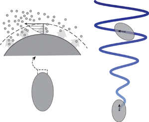
Figure 1. Self-propulsion of an elliptical disk uniformly releasing chemical solutes in a Newtonian solvent, where  $\boldsymbol {e}_{x},\boldsymbol {e}_{y}$ denotes the laboratory frame. The disk moves along an undulatory path with translational velocity $\boldsymbol {U}$, and the colour of the path is coded by the time $t$. The disk orientation $\boldsymbol {e}_s$ coinciding with its major axis deviates from $\boldsymbol {e}_{y}$ and $\boldsymbol {U}$ by angles $\theta$ and $\alpha$, respectively. The inset shows the induced slip velocity $\boldsymbol {u}_s$ by local solute gradients within a thin boundary layer of thickness $h \ll b$. Here, $\boldsymbol {n}$ denotes the unit normal vector pointing away from the disk surface. All the variables here are dimensionless.
We now describe the phoretic dynamics of the elliptical disk and the associated governing equations (Anderson Reference Anderson1989; Michelin et al. Reference Michelin, Lauga and Bartolo2013). The disk's surface  $\varGamma _d$ uniformly emits or absorbs solutes at a constant rate $\bar {A}$ (activity), hence
 \begin{equation} \bar{D}\boldsymbol{n} \boldsymbol{\cdot} \boldsymbol{\nabla} \bar{c}|_{\varGamma_d}=-\bar{A}. \end{equation}
Here,  $\bar {c}$ is the solute concentration, $\bar {D}$ denotes the molecular diffusivity of the solute, and $\boldsymbol {n}$ is the unit outward normal at the surface. Positive or negative $\bar {A}$ corresponds to the solute emission or absorption at the disk surface, respectively. The solute interacts with the disk surface through a short-range potential, and here we focus on the classical thin-interaction-layer limit $h \ll \bar {b}$, with $h$ the thickness of the interaction layer. Within this layer, the slip velocity along the disk surface induced by the local tangential solute gradients (Anderson Reference Anderson1989) reads
 \begin{equation} \bar{\boldsymbol{u}}_s|_{\varGamma_d} = \bar{M}\,\boldsymbol{\nabla}_s \bar{c}, \end{equation}
where  $\bar {\boldsymbol {u}}_s$ indicates the slip velocity, $\boldsymbol {\nabla }_s = (\boldsymbol {I} -\boldsymbol {n} \boldsymbol {n}) \boldsymbol {\cdot }\boldsymbol {\nabla }$ is the surface gradient operator, and $\bar {M}$ denotes the phoretic mobility coefficient. The coefficient $\bar {M}$ determines the chemotactic direction of the phoretic swimmer. For active droplets, $\bar {M}$ can be adjusted by tuning the relationship between surface tension and chemical solute, as shown by recent experiments (Wentworth et al. Reference Wentworth, Castonguay, Moerman, Meredith, Balaj, Cheon and Zarzar2022): $\bar {M}>0$ when they are positively correlated, and $\bar {M}<0$ when negatively correlated. Prior studies (Michelin et al. Reference Michelin, Lauga and Bartolo2013; Hu et al. Reference Hu, Lin, Rafai and Misbah2019) revealed that spontaneous symmetry-breaking propulsion is present only when $\bar {A}\bar {M}>0$; in other cases, the disk remains stable. Without loss of generality, our analysis focuses on $\bar {A}>0$ and $\bar {M}>0$, but the results will remain in the converse scenarios. Also, we assume that the inertia of both fluid and disk is negligible compared to the viscous force because the Reynolds number $Re$ is typically small in the experiments (Peddireddy et al. Reference Peddireddy, Kumar, Thutupalli, Herminghaus and Bahr2012; Maass et al. Reference Maass, Krüger, Herminghaus and Bahr2016; de Blois et al. Reference de Blois, Reyssat, Michelin and Dauchot2019; Hokmabad et al. Reference Hokmabad, Dey, Jalaal, Mohanty, Almukambetova, Baldwin, Lohse and Maass2021, Reference Hokmabad, Agudo-Canalejo, Saha, Golestanian and Maass2022; Michelin Reference Michelin2023). Hence the fluid flow surrounding the disk can be described approximately by the Stokes equation.
In the following, we introduce the dimensionless governing equations. We choose  $\bar {A} \bar {M}/\bar {D}$, $\bar {b}$ and $\bar {b}\bar {A}/\bar {D}$, respectively, as the characteristic velocity $\bar {\mathcal {V}}$, length and concentration for the non-dimensionalization. All variables below are dimensionless unless specified otherwise. The dimensionless equations for the velocity $\boldsymbol {u}$, pressure $p$ and concentration $c$ are
 $$\begin{gather} \boldsymbol{\nabla} \boldsymbol{\cdot} \boldsymbol{\sigma} = \boldsymbol{0},\quad \boldsymbol{\nabla} \boldsymbol{\cdot}\boldsymbol{u} = 0, \end{gather}$$
 $$\begin{gather}\frac{\partial c}{\partial t} + \boldsymbol{u} \boldsymbol{\cdot}\boldsymbol{\nabla} c = \frac{1}{Pe}\,\Delta c, \end{gather}$$
where  $Pe = \bar {A}\bar {M}\bar {b}/\bar {D}^2$ measures the ratio of flow advection to solute diffusion, and $\boldsymbol {\sigma } = -p\boldsymbol {I}+ \boldsymbol {\nabla } \boldsymbol {u} + (\boldsymbol {\nabla } \boldsymbol {u})^{{\rm T}}$ is the hydrodynamic stress tensor. At the disk surface, the constant flux boundary condition (2.1) for the concentration reads
 \begin{equation} \boldsymbol{n} \boldsymbol{\cdot}\boldsymbol{\nabla} c|_{\varGamma_d} =-1. \end{equation}
It is known that (2.4) does not support a steady-state solution within a 2-D infinite domain due to the logarithmic divergence (Sondak et al. Reference Sondak, Hawley, Heng, Vinsonhaler, Lauga and Thiffeault2016; Yariv Reference Yariv2017; Kailasham & Khair Reference Kailasham and Khair2023). To resolve this issue, we consider a circular fluid domain with a finite radius  $R$, and prescribe on its exterior $\varGamma _o$ that
 \begin{equation} c|_{\varGamma_o} = 0. \end{equation}
Following Hu et al. (Reference Hu, Lin, Rafai and Misbah2019) and Li (Reference Li2022), here we set  $R = 200$. In fact, we also examine the convergence of numerical results with respect to the domain size $R$, and reveal that the chosen $R$ is sufficiently large to ensure that the disk motion remains unaffected, as depicted in figure 13 of Appendix C.
We perform numerical simulations in the frame co-moving with the disk centre. Hence the boundary conditions for the velocity at the disk surface  $\varGamma _d$ and the outer boundary $\varGamma _o$ are
 $$\begin{gather} \boldsymbol{u} |_{\varGamma_d} = \boldsymbol{u}_s + \boldsymbol{\varOmega} \times (\boldsymbol{x}_s - \boldsymbol{x}_c), \end{gather}$$
 $$\begin{gather}\boldsymbol{u} |_{\varGamma_o} =-\boldsymbol{U}, \end{gather}$$
where  $\boldsymbol {u}_s = \boldsymbol {\nabla }_s c$ is the slip velocity at the disk surface, and $\boldsymbol {x}_s$ and $\boldsymbol {x}_c$ denote the coordinates of a general point at the disk surface and the disk centre, respectively. Here, $\boldsymbol {U}$ and $\boldsymbol {\varOmega }$ denote the translational and rotational velocities of the disk, respectively, which are determined by the force-free and torque-free conditions (Lauga & Powers Reference Lauga and Powers2009)
 $$\begin{gather}
\boldsymbol{F}=\int_{\varGamma_d}\boldsymbol{n}\boldsymbol{\cdot} \boldsymbol{\sigma}\,\mathrm{d} l =\mathbf{0},
\end{gather}$$
$$\begin{gather}
\boldsymbol{F}=\int_{\varGamma_d}\boldsymbol{n}\boldsymbol{\cdot} \boldsymbol{\sigma}\,\mathrm{d} l =\mathbf{0},
\end{gather}$$ $$\begin{gather}
%\boldsymbol{T} = \int (\boldsymbol{x}_s - \boldsymbol{x}_c) \times (\boldsymbol{n} \boldsymbol{\cdot} \boldsymbol{\sigma})\, \int_{\varGamma_d} \mathrm{d} l = \boldsymbol{0}.
\boldsymbol{T}=\int_{\varGamma_d}(\boldsymbol{x}_s-\boldsymbol{x}_c) \times (\boldsymbol{n}\boldsymbol{\cdot} \boldsymbol{\sigma})\,\mathrm{d} l =\mathbf{0}.
\end{gather}$$
$$\begin{gather}
%\boldsymbol{T} = \int (\boldsymbol{x}_s - \boldsymbol{x}_c) \times (\boldsymbol{n} \boldsymbol{\cdot} \boldsymbol{\sigma})\, \int_{\varGamma_d} \mathrm{d} l = \boldsymbol{0}.
\boldsymbol{T}=\int_{\varGamma_d}(\boldsymbol{x}_s-\boldsymbol{x}_c) \times (\boldsymbol{n}\boldsymbol{\cdot} \boldsymbol{\sigma})\,\mathrm{d} l =\mathbf{0}.
\end{gather}$$In other words, the total force and torque exerted on the disk swimmer are zero. The initial condition is zero velocity, pressure and concentration within the domain. Equations (2.3a,b)–(2.8) form the complete set of governing equations for an elliptical phoretic disk in the frame co-moving with the disk.
2.2. Numerical method
We solve numerically the governing equations, using a finite-element method solver implemented in the commercial package COMSOL Multiphysics (I-Math, Singapore). We adopt the moving mesh technique to tackle the deformation of the fluid domain caused by disk rotation. Taylor–Hood and quadratic Lagrange elements are employed to discretize the flow field  $(\boldsymbol {u}, p)$ and the concentration $c$, respectively. The computational domain is discretized by approximately 85 000–127 000 triangular elements, and the mesh is refined locally near the disk. Our COMSOL implementations are validated extensively against several published datasets, as shown in Appendix A.
3. Linear stability analysis
Prior studies reveal that a chemically isotropic disk/droplet possesses a stable stationary state at a sufficiently low  $Pe$. As $Pe$ grows beyond a critical value, an instability arises, leading the disk/droplet to swim autonomously (Hu et al. Reference Hu, Lin, Rafai and Misbah2019; Morozov & Michelin Reference Morozov and Michelin2019b; Li Reference Li2022). Our numerical results indicate that the elliptical disk here exhibits analogous behaviour, hence we conduct an LSA to examine the onset of instability at a critical Péclet number ${Pe}_c^{(1)}$.
We first decompose the space- ( $\boldsymbol {x}$) and time-dependent state variables $(c, \boldsymbol {u}, p)$ into the sum of a base state and a perturbation state as
 $$\begin{gather} c ( \boldsymbol{x}, t) = c_b ( \boldsymbol{x}) + c^{\prime} ( \boldsymbol{x}, t), \end{gather}$$
 $$\begin{gather}\boldsymbol{u} ( \boldsymbol{x}, t) = \boldsymbol{u}_b ( \boldsymbol{x}) + \boldsymbol{u}^{\prime} ( \boldsymbol{x}, t), \end{gather}$$
 $$\begin{gather}p ( \boldsymbol{x}, t) = p_b ( \boldsymbol{x}) + p^{\prime} ( \boldsymbol{x}, t), \end{gather}$$
where the subscript  $b$ denotes base-state fields, and the primed variables are infinitesimal perturbations. The base state can be obtained numerically. By substituting (3.1) into (2.3a,b) and (2.4), and retaining linear terms, we obtain
 $$\begin{gather} \boldsymbol{\nabla} \boldsymbol{\cdot} \boldsymbol{\sigma}^{\prime} = \boldsymbol{0},\quad \boldsymbol{\nabla}\boldsymbol{\cdot} \boldsymbol{u}^{\prime} = 0, \end{gather}$$
 $$\begin{gather}\frac{\partial c^{\prime}}{\partial t} + \boldsymbol{u}_b \boldsymbol{\cdot}\boldsymbol{\nabla} c^{\prime} + \boldsymbol{u}^{\prime} \boldsymbol{\cdot}\boldsymbol{\nabla} c_b = \frac{1}{Pe}\,\Delta c^{\prime}. \end{gather}$$
Note that  $\boldsymbol {u}_b ( \boldsymbol {x}) = \boldsymbol {0}$ for a stationary circular disk, while for its elliptical counterpart, $\boldsymbol {u}_b ( \boldsymbol {x}) \neq \boldsymbol {0}$ due to the anisotropic concentration distribution at the disk surface (see figure 6a). The perturbations are assumed to vary exponentially in time with a complex growth rate $\lambda = \lambda _r + i\lambda _i$, i.e.
 $$\begin{gather} c^{\prime} ( \boldsymbol{x}, t) = \hat{c} ( \boldsymbol{x}) \exp (\lambda t) , \end{gather}$$
 $$\begin{gather}\boldsymbol{u}^{\prime} ( \boldsymbol{x}, t) = \hat{\boldsymbol{u}} ( \boldsymbol{x}) \exp (\lambda t), \end{gather}$$
 $$\begin{gather}p^{\prime} ( \boldsymbol{x}, t) = \hat{p} ( \boldsymbol{x}) \exp (\lambda). \end{gather}$$
Consequently, (3.2a,b) and (3.3) can be reformulated to
 $$\begin{gather} \boldsymbol{\nabla}\boldsymbol{\cdot} \hat{\boldsymbol{\sigma}} = \boldsymbol{0},\quad \boldsymbol{\nabla}\boldsymbol{\cdot}\hat{\boldsymbol{u}} = 0, \end{gather}$$
 $$\begin{gather}\lambda \hat{c} + \boldsymbol{u}_b \boldsymbol{\cdot}\boldsymbol{\nabla} \hat{c} + \hat{\boldsymbol{u}} \boldsymbol{\cdot} \boldsymbol{\nabla} c_b = \frac{1}{Pe}\,\Delta \hat{c}. \end{gather}$$
By expanding the translational and rotational velocities similarly, we arrive at  $\boldsymbol {U} = \boldsymbol {U}_b + \hat {\boldsymbol {U}} \exp (\lambda t)$ and $\boldsymbol {\varOmega } = \boldsymbol {\varOmega }_b + \hat {\boldsymbol {\varOmega }} \exp (\lambda t)$. Substituting these with (3.1) into (2.5)–(2.7) enables us to derive the boundary conditions for $\hat {c}$ and $\hat {\boldsymbol {u}}$ at the disk surface and outer boundary:
 $$\begin{gather}
%\boldsymbol{n} \boldsymbol{\cdot}\boldsymbol{\nabla} \hat{c}|_{\varGamma_p} = 0,\quad \hat{c}|_{\varGamma_o} = 0,
\boldsymbol{n}\boldsymbol{\cdot}\boldsymbol{\nabla} \hat{c} |_{\varGamma_d} =0, \quad \hat{c}|_{\varGamma_o}=0,
\end{gather}$$
$$\begin{gather}
%\boldsymbol{n} \boldsymbol{\cdot}\boldsymbol{\nabla} \hat{c}|_{\varGamma_p} = 0,\quad \hat{c}|_{\varGamma_o} = 0,
\boldsymbol{n}\boldsymbol{\cdot}\boldsymbol{\nabla} \hat{c} |_{\varGamma_d} =0, \quad \hat{c}|_{\varGamma_o}=0,
\end{gather}$$ $$\begin{gather}
%\hat{\boldsymbol{u}}|_{\varGamma_p} = \boldsymbol{\nabla}_s \hat{c} + \hat{\boldsymbol{\varOmega}} \times (\boldsymbol{x}_s-\boldsymbol{x}_c),\quad \hat{\boldsymbol{u}}|_{\varGamma_o} =-\hat{\boldsymbol{U}}.
\hat{\boldsymbol{u}}|_{\varGamma_d} = \boldsymbol{\nabla}_s \hat{c} + \hat{\boldsymbol{\varOmega}}\times (\boldsymbol{x}_s - \boldsymbol{x}_c ), \quad \hat{\boldsymbol{u}}|_{\varGamma_o} = -\hat{\boldsymbol{U}}.
\end{gather}$$
$$\begin{gather}
%\hat{\boldsymbol{u}}|_{\varGamma_p} = \boldsymbol{\nabla}_s \hat{c} + \hat{\boldsymbol{\varOmega}} \times (\boldsymbol{x}_s-\boldsymbol{x}_c),\quad \hat{\boldsymbol{u}}|_{\varGamma_o} =-\hat{\boldsymbol{U}}.
\hat{\boldsymbol{u}}|_{\varGamma_d} = \boldsymbol{\nabla}_s \hat{c} + \hat{\boldsymbol{\varOmega}}\times (\boldsymbol{x}_s - \boldsymbol{x}_c ), \quad \hat{\boldsymbol{u}}|_{\varGamma_o} = -\hat{\boldsymbol{U}}.
\end{gather}$$
Note that  $\boldsymbol {U}_b$ and $\boldsymbol {\varOmega }_b$ disappear in (3.8), corresponding to a stationary disk of the base state. The force-free and torque-free conditions still hold as
 $$\begin{gather}
\hat{\boldsymbol{F}}=\int_{\varGamma_d}\boldsymbol{n} \boldsymbol{\cdot}
\hat{\boldsymbol{\sigma}}\,\mathrm{d} l =\mathbf{0},
\end{gather}$$
$$\begin{gather}
\hat{\boldsymbol{F}}=\int_{\varGamma_d}\boldsymbol{n} \boldsymbol{\cdot}
\hat{\boldsymbol{\sigma}}\,\mathrm{d} l =\mathbf{0},
\end{gather}$$ $$\begin{gather}
%\hat{\boldsymbol{T}} = \int (\boldsymbol{x}_s - \boldsymbol{x}_c) \times (\boldsymbol{n} \boldsymbol{\cdot} \hat{\boldsymbol{\sigma}})\,\int_{\varGamma_p} \mathrm{d} l = \boldsymbol{0}.
\hat{\boldsymbol{T}}=\int_{\varGamma_d}(\boldsymbol{x}_s-\boldsymbol{x}_c) \times (\boldsymbol{n}\boldsymbol{\cdot} \hat{\boldsymbol{\sigma}})\,\mathrm{d} l =\mathbf{0}.
\end{gather}$$
$$\begin{gather}
%\hat{\boldsymbol{T}} = \int (\boldsymbol{x}_s - \boldsymbol{x}_c) \times (\boldsymbol{n} \boldsymbol{\cdot} \hat{\boldsymbol{\sigma}})\,\int_{\varGamma_p} \mathrm{d} l = \boldsymbol{0}.
\hat{\boldsymbol{T}}=\int_{\varGamma_d}(\boldsymbol{x}_s-\boldsymbol{x}_c) \times (\boldsymbol{n}\boldsymbol{\cdot} \hat{\boldsymbol{\sigma}})\,\mathrm{d} l =\mathbf{0}.
\end{gather}$$
Equations (3.5a,b)–(3.9) define an eigenvalue problem. The stability of the base state is determined by the eigenvalue with the largest real part  $\lambda _r^0$, namely the leading eigenvalue, and the corresponding perturbations $(\hat {\boldsymbol {u}}, \hat {p}, \hat {c})^{\rm T}$ are called leading eigenmodes. The base state is stable when $\lambda _r^0 < 0$, but unstable when $\lambda _r^0 > 0$. The Péclet number at which $\lambda _r^0 = 0$ is precisely the critical Péclet number ${Pe}_c^{(1)}$ signifying the transition from a stationary state to steady propulsion. Unless stated otherwise, the eigenvalues mentioned below refer to the leading eigenvalues, and the superscript $0$ is omitted for simplicity. We solve the eigenvalue problem with COMSOL using the eigenvalue solver ARPACK. The validation of our approach is demonstrated in Appendix A.
4. Results
4.1. Diverse behaviours of an elliptical phoretic disk
By increasing  $Pe$, we demonstrate the diverse $Pe$-dependent behaviours of a disk with eccentricity $e=0.87$. For a sufficiently small $Pe$ below a critical value ${Pe}_c^{(1)}$, the disk undergoes transient rotation before recovering a stationary state. When $Pe$ goes above ${Pe}_c^{(1)}$, e.g. $Pe = 0.4$, the stationary state transits into steady propulsion, in which the fore–aft symmetry in the concentration profile is broken (see figure 2f), and the resultant concentration polarity induces a rectilinear motion with a constant swimming speed, as depicted in figure 2(a). Further increasing $Pe$ to $0.62$, the directed motion loses its stability, leading to a secondary instability characterized by spontaneous chiral symmetry breaking. Consequently, the disk repeatedly traces a circular path, exhibiting spontaneous rotation (clockwise, in this instance), as depicted in figure 2(b). This regime featuring circular trajectory and self-rotation is called the orbiting regime. Hu et al. (Reference Hu, Lin, Rafai and Misbah2019) and Li (Reference Li2022) observed analogous circular trajectories executed by circular swimmers without self-rotation. At $Pe = 10$, the elliptical disk favours a wave-like trajectory after a transient period of swimming straight forwards (see figure 2c). From the viewpoint of the frame co-moving with the disk centre, the disk swings periodically like a pendulum (see figure 2g). This swimming behaviour is analogous to that exhibited by an active prolate double-core droplet that moves along an undulatory trajectory (Hokmabad et al. Reference Hokmabad, Baldwin, Krüger, Bahr and Maass2019). Li (Reference Li2022) also reported that a high- $Pe$ active drop swims along a periodic zigzag trajectory. As $Pe$ increases to $25$, the elliptical disk surprisingly recovers to steady propulsion, as illustrated in figure 2(d). In correspondence, chiral symmetry recovers. Unlike the ballistic motion after rotation at low $Pe$, the disk here travels straight from the onset of instability without any rotation. The steady propulsion becomes unstable at a higher $Pe$, e.g. $Pe = 33$; accordingly, the disk swims straight forwards at an oscillating speed (see figure 12 in Appendix B). Hu et al. (Reference Hu, Lin, Rafai and Misbah2022) and Kailasham & Khair (Reference Kailasham and Khair2022) identified the similar motion of a 3-D isotropic phoretic particle in an axisymmetric set-up, where the particle does not rotate, and the flow and concentration fields are symmetric about an axis parallel to the particle's translational direction. Figure 2(e) indicates that the disk enters into a chaotic regime characterized by an erratic trajectory at $Pe = 60$. In contrast to frequent intermittency and random walk occurring in the chaotic regime for a circular disk, as observed by Hu et al. (Reference Hu, Lin, Rafai and Misbah2019), the change of velocity in both direction and magnitude experienced by the elliptical disk is not drastic, yielding a less chaotic trajectory.

Figure 2. An elliptical disk of eccentricity  $e = 0.87$ follows typical trajectories depending on $Pe$: (a) steady, (b) orbiting, (c) periodic, (d) steady, and (e) chaotic. The colour of a trajectory is coded by the time $t$. Green and red arrows denote the direction of the translational velocity $\boldsymbol {U}$ and the disk orientation $\boldsymbol {e}_s$, respectively. (f) Polarized concentration distribution with respect to $\boldsymbol {e}_s$ at $Pe = 0.4$. (g) Periodic pendulum-like swinging of the disk at $Pe =10$ in the frame co-moving with its centre. The star and triangle symbols marked in (g) denote the two distinct moments when the disk reaches the peak and trough of its trajectory, respectively, as shown in (c).
Having observed distinct swimming behaviours of a disk with a specific eccentricity at varying  $Pe$, we then systematically examine how the eccentricity $e$ affects these $Pe$-dependent behaviours. The phase diagram in figure 3 shows that shifts in $Pe$-dependent behaviours of an elliptical disk with $e$ below $0.75$ resemble those of a circular counterpart ( $e = 0$). The elliptical disk executes successively stationary, steady, periodic and chaotic motion with increasing $Pe$. As $e$ exceeds $0.75$, the disk exhibits richer dynamics: the orbiting motion emerges with broken chiral symmetry. In fact, we have also explored the scenarios at $e > 0.9$, e.g. $e = 0.96$, and observed that the swimming dynamics of the elliptical disk is almost dominated by orbiting and chaotic regimes (not shown here). These two regimes have been revealed in the current phase diagram, hence the characteristic locomotory modes can be well captured in the range of $e$ considered.

Figure 3. Phase diagram characterizing the behaviours of an elliptical phoretic disk depending on its eccentricity  $e$ and the Péclet number $Pe$. It shows five regimes: stationary, steady, orbiting, periodic and chaotic. The solid line denotes the LSA prediction.
We further discern from the phase diagram that the variation of  $e$ categorizes certain identified swimming patterns into two types. In the stationary or steady swimming regime, the aforementioned observations indicate that the disk experiences transient rotation before recovering a stationary state or retaining a steady motion (see figure 2). Nevertheless, these situations are applicable only at a higher $e$, clearly distinguished by light-coloured symbols. When $e < 0.75$, the disk remains stationary or swims straight without any rotation. Besides, two types of periodic motions are depicted in the phase diagram: (1) a disk swings along a wavy trajectory (light-coloured squares); (2) a disk swims straight at an oscillating swimming speed (dark-coloured squares). The former and the latter are termed swinging and straight periodic motions, respectively.
4.2. Spontaneous steady propulsion triggered by instability
Upon gaining a general understanding of the phase diagram, we then explore the detailed swimming dynamics within each regime. We first focus on the transition from the stationary to steady swimming regime. The disk is stationary in the base state. As  $Pe$ exceeds ${Pe}_c^{(1)}$, an instability arises, and the disk sets into steady propulsion along its major axis. Here, we perform a LSA, as introduced in § 3, to identify quantitatively ${Pe}_c^{(1)}$ and its dependence on the disk shape. The ${Pe}_c^{(1)}$ value predicted by the LSA decreases monotonically with $e$, as depicted by the solid line in figure 3. Figure 4(a) depicts the concentration field $\hat {c}$ of the eigenmode at ${Pe}_c^{(1)} \approx 0.42$ for $e = 0.55$. We see that the symmetry of the base concentration field $\hat {c}$ is broken in the direction of the major axis at ${Pe}_c^{(1)}$. The fore–aft asymmetric concentration distribution induces a downward slip flow, as shown by the flow field $\hat {\boldsymbol {u}}$ of the eigenmode in figure 4(b), driving the steady motion of the disk along its major axis. In close proximity to ${Pe}_c^{(1)}$, the swimming speed $U_{mg}$ is proportional to $\sqrt {Pe-{Pe}_c^{(1)}}$ (see figure 4c), implying that the instability occurs through a supercritical pitchfork bifurcation. This is parallel to the observation of Hu et al. (Reference Hu, Lin, Rafai and Misbah2019) and Li (Reference Li2022).

Figure 4. Eigenmodes at the critical Péclet number  ${Pe}_c^{(1)} \approx 0.42$ for an elliptical disk with $e = 0.55$. The eigenmode is characterized by (a) the perturbation concentration $\hat {c}$, and (b) the perturbation velocity $\hat {\boldsymbol {u}}$ (red arrows) and its $y$ component $\hat {v}$ (colour map). (c) Dependence of time-averaged disk speed $\langle U_{mg} \rangle$ on $Pe-{Pe}_c^{(1)}$ at varying $e$. In the vicinity of ${Pe}_c^{(1)}$, $\langle U_{mg} \rangle$ is proportional to $\sqrt {Pe-{Pe}_c^{(1)}}$. (d) The $Pe$-dependent growth rate $\lambda$ based on the LSA and $\lambda _e= \lambda _c + \lambda _d$ derived from the concentration perturbation equation (3.6). The latter comprises the contributions $\lambda _c$ and $\lambda _d$ from advection and diffusion, respectively.
We further probe the physical mechanism underlying the instability by adopting an approach resembling the energy budget analysis (Bendiksen Reference Bendiksen1985; Abubakar & Matar Reference Abubakar and Matar2022). By taking an inner product, denoted by  $(\cdot, \cdot )$, of (3.6) with $\hat {c}$ in the $L^2$ space, we arrive at
 \begin{equation} (\lambda \hat{c}, \hat{c}) + (\boldsymbol{u}_b \boldsymbol{\cdot}\boldsymbol{\nabla} \hat{c}, \hat{c}) + (\hat{\boldsymbol{u}} \boldsymbol{\cdot}\boldsymbol{\nabla} c_b, \hat{c}) = \frac{1}{Pe}\,(\Delta \hat{c}, \hat{c}). \end{equation}
Using integration by parts, the divergence-free condition in (3.5a,b), and the boundary conditions (3.7) and (3.8), we derive
 $$\begin{gather}
%( \boldsymbol{u}_b \boldsymbol{\cdot}\boldsymbol{\nabla} \hat{c}, \hat{c}) = \frac{1}{2}\,(\boldsymbol{n} \boldsymbol{\cdot}\boldsymbol{u}_b, \hat{c}^2)_{\varGamma_p} +\frac{1}{2}\,(\boldsymbol{n} \boldsymbol{\cdot} \boldsymbol{u}_b, \hat{c}^2)_{\varGamma_o} = 0,
(\boldsymbol{u}_b \boldsymbol{\cdot} \boldsymbol{\nabla} \hat{c}, \hat{c}) = \tfrac{1}{2}(\boldsymbol{n}\boldsymbol{\cdot}\boldsymbol{u}_b ,\hat{c}^2)_{\varGamma_d} + \tfrac{1}{2}(\boldsymbol{n}\boldsymbol{\cdot}\boldsymbol{u}_b ,\hat{c}^2)_{\varGamma_o} = 0,
\end{gather}$$
$$\begin{gather}
%( \boldsymbol{u}_b \boldsymbol{\cdot}\boldsymbol{\nabla} \hat{c}, \hat{c}) = \frac{1}{2}\,(\boldsymbol{n} \boldsymbol{\cdot}\boldsymbol{u}_b, \hat{c}^2)_{\varGamma_p} +\frac{1}{2}\,(\boldsymbol{n} \boldsymbol{\cdot} \boldsymbol{u}_b, \hat{c}^2)_{\varGamma_o} = 0,
(\boldsymbol{u}_b \boldsymbol{\cdot} \boldsymbol{\nabla} \hat{c}, \hat{c}) = \tfrac{1}{2}(\boldsymbol{n}\boldsymbol{\cdot}\boldsymbol{u}_b ,\hat{c}^2)_{\varGamma_d} + \tfrac{1}{2}(\boldsymbol{n}\boldsymbol{\cdot}\boldsymbol{u}_b ,\hat{c}^2)_{\varGamma_o} = 0,
\end{gather}$$ $$\begin{gather}( \hat{\boldsymbol{u}} \boldsymbol{\cdot}\boldsymbol{\nabla} c_b, \hat{c}) =-(c_b, \hat{\boldsymbol{u}} \boldsymbol{\cdot}\boldsymbol{\nabla} \hat{c}), \end{gather}$$
 $$\begin{gather}\frac{1}{Pe}\,(\Delta \hat{c}, \hat{c}) =-\frac{1}{Pe}\,\| \boldsymbol{\nabla} \hat{c} \|^2, \end{gather}$$
with  $\| \cdot \|$ denoting the $L^2$-norm. By substituting (4.2) into (4.1), we obtain
 \begin{equation} \lambda_e = \lambda_c+\lambda_d, \end{equation}
with
 $$\begin{gather} \lambda_c = \frac{(c_b, \hat{\boldsymbol{u}} \boldsymbol{\cdot}\boldsymbol{\nabla} \hat{c})}{(1, \hat{c}^2)}, \end{gather}$$
 $$\begin{gather}\lambda_d =- \frac{\| \boldsymbol{\nabla} \hat{c} \|^2}{(Pe, \hat{c}^2)}. \end{gather}$$
Here, the growth rate  $\lambda _e$ is introduced in (4.3) to be distinguished from $\lambda$ obtained by the LSA. Also, $\lambda _c$ and $\lambda _d$ represent the contributions of advection and diffusion to $\lambda _e$, respectively. For a steady motion, the imaginary part of the growth rate vanishes, thus the growth rate has only its real part, e.g. $\lambda = \lambda _r$. Figure 4(d) shows that $\lambda _e$ and $\lambda$ lie on top of each other, giving us the confidence to analyse the dominant physical ingredient that drives the instability using (4.3). We infer naturally from (4.3) that $\lambda _c$ is responsible for $\lambda _e$ turning positive by realizing that $\lambda _d$ is consistently negative, as confirmed by figure 4(d). Hence, as anticipated, advection drives the instability and diffusion dampens the perturbation, and the balance between them dominates the phoretic dynamics of the elliptical disk: at small $Pe$, diffusion dominates, and its homogenizing effect maintains a fore–aft symmetric solute distribution. As $Pe$ grows beyond ${Pe}_c^{(1)}$, advection suppresses diffusion and amplifies the asymmetric solute disturbance. The slip flows triggered by the asymmetric concentration distribution drive the disk to swim spontaneously.
Next, we analyse the steady propulsion of the autophoretic disk. We show in figures 5(a,c) that the elliptical disk with  $e = 0.55$ swims as a puller, attracting the fluid from its front and rear at $Pe = 0.5$. In contrast, it becomes a neutral-type swimmer at $Pe=1.5$, as indicated in figures 5(b,c). In retrospect, Suda et al. (Reference Suda, Suda, Ohmura and Ichikawa2021) reported an analogous transition from a puller swimming straight into a pusher-type swimmer executing unsteady curvilinear motion when $Pe$ increases. In that case, the droplet motion is triggered by the concentration gradient caused by a point source of surfactant at the surface. Besides, Li (Reference Li2022) observes that an active drop transits from a steady pusher to a mixed pusher–puller propelling unsteadily as $Pe$ grows. In the case of these droplet swimmers, the switching of their disturbance flow occurs as they go from steady to unsteady motion. Morozov & Michelin (Reference Morozov and Michelin2019a) describes a $Pe$-dependent neutral-to-pusher transition for a 3-D axisymmetric droplet impelling steadily. Notably, this transition occurs without a shift in the droplet's swimming pattern, resembling that exhibited by the disk swimmer here. We examine further the flow field in the frame co-moving with the disk throughout the whole steady swimming regime, and summarize these results in a phase diagram in figure 5(d). It is found that a circular ( $e = 0$) or nearly circular disk can be only a neutral swimmer, and the puller-to-neutral transition emerges as $e\geq 0.20$. The critical Péclet number $Pe_t$ signifying this transition depends monotonically on $e$, as indicated by the dashed line. When $e > 0.65$, the transition disappears and the disk swims solely as a puller. In fact, this peculiar transformation can be understood by examining the solute distribution at the disk surface, as discussed below. For visualization purposes, we normalize the concentration via $\tilde {c} = 0.3 (c_{max}-c)/(c_{max}-c_{min})$, where $c_{max}$ and $c_{min}$ denote the maximum and minimum concentrations at the disk surface, respectively.

Figure 5. (a) A puller-type steady swimmer at  $Pe = 0.5$ transitions to (b) a neutral-type counterpart at $Pe = 1.5$, where the eccentricity $e$ is $0.55$. The flow fields are shown in the frame co-moving with the disk. Black arrows denote swimming direction. The colour maps indicate the distribution of $c$. The stagnation point ${P}$ coincides with the peak of $c$ at the disk surface. (c) Polar velocity magnitude $\boldsymbol {u}_s \boldsymbol {\cdot } \boldsymbol {t}$ at the disk surface, following the definition in Downton & Stark (Reference Downton and Stark2009). Here, $\beta$ is the polar angle with respect to the disk orientation $\boldsymbol {e}_s$, with $\boldsymbol {t}$ the corresponding unit tangent vector. (d) $Pe\unicode{x2013}e$ phase diagram shows puller-type and neutral-type steady swimmers demarcated by the dashed line. Solid lines separate regimes identified in figure 3.
We demonstrate in figures 6(a,d) the bimodal distribution of normalized concentration caused by the curvature variation of the disk surface in the base state ( $Pe = 0.3$). The maximum normalized concentration $\tilde {c}_{max}$ is located at the left vertex of the minor axis corresponding to $\beta = 90^{\circ }$, where $\beta$ denotes the polar angle with respect to $\boldsymbol {e}_s$. Here, we consider only the left half of the disk ( $\beta \in [0, 180^{\circ }]$) for its symmetry. At $Pe = 0.5$, the base state loses stability and solutes are advected toward the disk's rear ( $\beta = 180^{\circ }$). Correspondingly, the position of $c_{max}$ migrates rearwards from $\beta = 90^{\circ }$ to the stagnation point ${P}$, as depicted in figure 6(b). Considering that the slip velocity $\boldsymbol {u}_s = \boldsymbol {\nabla }_s c$ is directed from low to high concentration at the disk surface, the fluid is attracted from the front and rear of the elliptical disk to the stagnation position ${P}$, forming a puller-type swimmer (see figure 5a). As $Pe$ increases to $1.5$, the enhanced convective transport of solutes causes the shift from a bimodal to a polarized concentration profile with the peak concentration located at $\beta = 180^{\circ }$ (see figure 6c). Correspondingly, the slip flow induced by the concentration gradient is driven from the front to the rear of the disk (see figure 6b), generating a prototypical neutral-type swimmer. We comment that as an elliptical disk swims steadily, a bimodal concentration profile at its surface yields a puller-type swimmer, while a polarized one leads to a neutral-type counterpart. Different from the elliptical disk, a circular disk has an isotropic base distribution of the solute ( $Pe = 0.3$), as shown in figures 6(e,g). For an unstable base state at $Pe = 1.5$, solutes are advected rearwards along the disk surface, leading to the direct transition from an isotropic to a polarized concentration profile. Hence the circular disk behaves as a neutral swimmer solely.

Figure 6. Normalized concentration at the surface of a disk swimming steadily: (a–c) for an elliptical disk with  $e = 0.55$ at $Pe = 0.3$, $0.5$ and $1.5$, respectively; (e,f) for a circular disk at $Pe = 0.3$ and $0.5$, respectively. Here, $c_{max}$ denotes the peak concentration at the disk surface. The stagnation point ${P}$ coincides with the location of $\tilde {c}_{max}$ at $Pe = 0.5$. (d) Transition from a bimodal to a polarized concentration distribution at the surface of an elliptical disk by increasing $Pe$. (g) Similar to (d), but for a circular disk with a transition from an isotropic solute distribution.
4.3. Chiral symmetry-breaking orbiting motion
Having observed the puller–neutral transition in the steady swimming regime, we direct our focus onto the chiral symmetry-breaking orbiting motion of the elliptical disk. Here, the disk swims approximately along a circular trajectory (see figure 2b) with rotational velocity  $\varOmega$. The time evolution of $\varOmega$ resembles that of $\alpha$ in figure 7(a) oscillating around a constant value: the constant value determines a globally circular trajectory, and the oscillations contribute to a locally undulatory trajectory. We find that the translational velocity $\boldsymbol {U}$ (green arrow in figure 2b) deviates from $\boldsymbol {e}_s$ (red arrow) by an angle $\alpha$ oscillating slightly around $15^{\circ }$ for $Pe=4$. In fact, the misalignment of $\boldsymbol {U}$ and $\boldsymbol {e}_s$ can be rationalized by examining the solute distribution $c(x,y)$ around the disk. Figure 7(b) illustrates $c(x,y)$ and streamlines at a specific moment $t = 5840$. The left–right asymmetry of the solute distribution about $\boldsymbol {e}_s$ gives rise to the asymmetric slip velocity, as reflected by the streamlines, hence causing diverging directions of $\boldsymbol {U}$ and $\boldsymbol {e}_s$. Besides, we notice that three stagnation points near the rear of the disk in figure 7(b) migrate gradually towards the rear with increasing $Pe$ in the orbiting regime (not shown here). Accordingly, the time-averaged $\langle \alpha \rangle = \int _0^{T} \alpha \,\mathrm {d}t /T$ within a time window $T$ decreases monotonically with $Pe$, as shown in the inset of figure 7(a). Intuitively, we infer that $\boldsymbol {U}$ is aligned with $\boldsymbol {e}_s$ ( $\alpha = 0$) as the three stagnation points coincide exactly at the rear of the disk, and indeed they do as $Pe$ grows beyond $14$ where the disk executes a steady motion, e.g. $Pe = 25$ (streamlines and concentration distribution are analogous to figure 5b).

Figure 7. (a) Time evolution of the angle  $\alpha$ between the translational velocity $\boldsymbol {U}$ and the disk orientation $\boldsymbol {e}_s$ as the elliptical disk with $e = 0.87$ approximately follows a circular trajectory for $Pe = 4$. The inset shows the monotonic decrease of the time-averaged $\alpha$ with $Pe$. (b) Solute distribution and streamlines at the instant $t = 5840$ marked in (a). Three hexagons denote the stagnation points at the rear of the disk.
The orbiting regime is characterized by the continuous rotation of an elliptical disk, which loses its chiral symmetry spontaneously. Conversely, a circular disk maintains this symmetry irrespective of the  $Pe$ value. In particular, for $Pe \in [9, 13]$, despite the asymmetric solute distribution and streamlines resembling those in figure 7(b) occasionally, the circular disk executes only a meandering motion (Hu et al. Reference Hu, Lin, Rafai and Misbah2019) without rotation. Ideally, a secondary stability analysis similar to the one performed above will help us to understand the mechanism for the shape-induced chiral symmetry breaking. This task is, however, technically challenging, and will be pursued in the future.
Notably, experiments on active droplets in a Hele-Shaw cell showed that the droplet preferred to avoid the concentration trail emitted by itself at earlier times, termed a self-avoiding walk phenomenon (Hokmabad et al. Reference Hokmabad, Dey, Jalaal, Mohanty, Almukambetova, Baldwin, Lohse and Maass2021). The elliptical disk here does not avoid similarly but instead repeats its previous trajectory, as shown in figure 2(b). The difference can be rationalized by a scaling analysis. We estimate that the time  $\bar {t}_d$ required for the concentration to decay to zero is of the order of $\bar {b}^2/\bar {D}$. The disk moves with speed $U_{mg} \bar {\mathcal {V}}$, hence the travelling time $\bar {t}_p$ taken to execute a circular trajectory of perimeter $\bar {L}_p$ is $\bar {L}_p/(U_{mg} \bar {\mathcal {V}})$, approximately. Recalling the definitions of $\bar {\mathcal {V}}$ and $Pe$ in § 2, we rewrite $\bar {t}_p$ as $\bar {L}_p\bar {b}/(U_{mg}\,Pe\,\bar {D})$. The ratio between these two time scales is
 \begin{equation} \frac{\bar{t}_p}{\bar{t}_d} = \frac{\bar{L}_p/\bar{b}}{U_{mg}\,Pe}. \end{equation}
At a specific  $Pe$, e.g. $Pe = 4$, in the orbiting regime, $\bar {t}_p /\bar {t}_d \approx 87.2 \gg 1$. This substantial ratio indicates that the disk swimmer can barely sense and thus avoid its own rapidly decaying chemical trace. In contrast, for a sufficiently larger $Pe$, we may observe the self-avoidance due to the significantly reduced travel time $t_p$ (Hokmabad et al. Reference Hokmabad, Dey, Jalaal, Mohanty, Almukambetova, Baldwin, Lohse and Maass2021; Hu et al. Reference Hu, Lin, Rafai and Misbah2022).
4.4. Periodic swinging
Typically, the orbiting motion transitions to periodic swinging (refer to figure 2c) as  $Pe$ increases, which will be analysed below. Figure 8(a) illustrates that the time-evolving rotational velocity $\varOmega$ of the disk with $e = 0.87$ at $Pe = 12.5$ is characterized by two phases. First, $\varOmega$ grows rapidly due to self-oscillation, and the dashed line connecting local peaks $\varOmega _{pk}$ of $\varOmega$ indicates an exponential growth of $\varOmega$ in time. This trend is confirmed by the linear relationship between $\log \varOmega _{pk}$ and $t$ shown in the inset of figure 8(a). Second, $\varOmega$ saturates nonlinearly to a periodic state with a constant amplitude $\varOmega _{mg}$. The sinusoidal-like variation of $\varOmega$ leads to a wave-like trajectory. We plot $\varOmega _{mg}^2$ as a function of $Pe$ near the critical $Pe \approx 13.5$ (star) in figure 8(b). The linear dependence of $\varOmega _{mg}^2$ on $Pe$ implies that the steady motion loses stability through a Hopf bifurcation. The critical $Pe$ signifies the boundary between the periodic swinging and steady motion. We further present in figure 8(c) the phase portrait in the $\varOmega$– $U$ plane, where the unstable spiral at the origin grows continuously to an elliptical stable limit circle, indicating the supercritical nature of the Hopf bifurcation. Notably, when $e< 0.87$, we observe a transition from steady to periodic swinging with increasing $Pe$, e.g. $e = 0.81$ (see figure 3). The Hopf bifurcation still holds for the onset of instability that triggers this transition.

Figure 8. (a) Time evolution of the rotational velocity  $\varOmega$ of an elliptical disk with $e = 0.87$ at $Pe =12.5$. The dashed line denotes certain local peaks $\varOmega _{pk}$ of $\varOmega$, and the inset shows the linear dependence of $\log \varOmega _{pk}$ on $t$. (b) Linear variation of $\varOmega _{mg}^2$ in $Pe$ near the critical $Pe\approx 13.5$ (star), where $\varOmega _{mg}$ denotes the constant amplitude of $\varOmega$ at $t > 5400$, as depicted by the dotted line in (a). The periodic motion recovers to steady propulsion as $Pe$ grows beyond the critical value. (c) Phase portrait in the $\varOmega$– $U$ plane, with the colour of the unstable spiral coded by $t$.
$t$.
4.5. Chaotic swimming dynamics
Finally, we analyse the chaotic motion of elliptical disks by examining their mean square displacement (MSD) and the velocity autocorrelation function (VAF). We calculate the  $\text {MSD} (\tau )$ of a disk (Michalet Reference Michalet2010) that depends on a time lag $\tau$ by
 \begin{equation} \text{MSD} (\tau) = \frac{1}{T-\tau}\int_{0}^{T-\tau}[\boldsymbol{r}(t+ \tau) -\boldsymbol{r}(t)]^2\,\mathrm{d} t, \end{equation}
where  $\boldsymbol {r} (t)$ denotes the time-dependent displacement of a disk relative to its original position. Clearly, combining a large time period $T$ and $\tau \ll T$ can improve the statistical confidence. We calculate VAF using
 \begin{equation} \text{VAF} (t) = \frac{1}{T}\int_0^{T} \frac{\boldsymbol{U} (t) \boldsymbol{\cdot}\boldsymbol{U} (t + \Delta t)}{| \boldsymbol{U} (t)|\, | \boldsymbol{U} (t+ \Delta t)|}\,\mathrm{d}t,\end{equation}
where a sufficiently large  $T$ is used to attain statistical invariance (Chen et al. Reference Chen, Chong, Liu, Verzicco and Lohse2021).
We examine how the eccentricity  $e$ of a disk affects its chaotic motion. First, we determine the shape-dependent ${Pe}_c^{(2)} (e)$ when chaos emerges. Then we investigate the chaotic dynamics at $Pe(e) = {Pe}_c^{(2)} (e) + 10$ above that threshold by a fixed offset, namely $10$ here. The corresponding MSD and VAF are depicted in figure 9(a). At early times, despite the diversity in the disk shape, they all swim persistently, resulting in the quadratically growing MSD in $\tau$. At long times, the disk shape considerably affects its phoretic movement, leading to a transition from a random-walking circular disk to a ballistically swimming elliptical counterpart. For the former, we reproduce perfectly its random walk behaviour as reported by Hu et al. (Reference Hu, Lin, Rafai and Misbah2019, Reference Hu, Lin, Rafai and Misbah2022) and Lin, Hu & Misbah (Reference Lin, Hu and Misbah2020), which features the linear scaling $\text {MSD} \propto \tau$ and the decorrelation in velocity $\boldsymbol {U}$ due to the rapidly changing swimming direction (see the inset). As the eccentricity $e$ increases to $0.1$, $\text {MSD} \varpropto \tau ^{1.5}$, reminiscent of the self-avoidance walk identified experimentally (Hokmabad et al. Reference Hokmabad, Dey, Jalaal, Mohanty, Almukambetova, Baldwin, Lohse and Maass2021). We wonder whether this growth scaling, ${\propto }\tau ^{1.5}$, results from the self-avoidance walk. By utilizing the scaling analysis mentioned above, we compare the decay time of the chemical $\bar {t}_d$ and the travelling time $\bar {t}_p$ of the disk, and find that $\bar {t}_p /\bar {t}_d \approx 40.8 \gg 1$ (see (4.5)), precluding self-avoidance here. At $e = 0.87$, the MSD's quadratic growth over lag time implies that the elliptical disk approximately executes the ballistic motion, as confirmed by the trajectory shown in figure 2(e). Accordingly, the VAF is almost constant in time, indicating a correlation in velocity $\boldsymbol {U}$. It is worth noting that Hu et al. (Reference Hu, Lin, Rafai and Misbah2022) and Morozov & Michelin (Reference Morozov and Michelin2019a) also found the quadratic variations of MSD for the chaotic swimming of a phoretic particle and an active droplet, respectively, under the axisymmetric assumption.

Figure 9. (a) Mean square displacement (MSD) and velocity autocorrelation function (VAF) for disks with different shapes at  ${Pe}_c^{(2)}+10$, where ${Pe}_c^{(2)}$ is the shape-dependent critical Péclet number corresponding to the onset of chaos. (b) The exponent $k$ of the power-law scaling $\text {MSD} \propto \tau ^k$ versus $e$. (c) Monotonic dependence of $k$ on $Pe$ for the disk of $e = 0.2$. (d) Chaotic trajectories (colour-coded by $t$) followed by an elliptical disk of $e = 0.2$ at $Pe = 8$, $27$ and $47$, respectively.
By probing further in figure 9(b) the exponent  $k$ of power-law scaling $\text {MSD} \propto \tau ^k$ at varying $e$, we notice that the normal diffusion ( $k = 1$) transitions to superdiffusion ( $k > 1$) as $e$ increases. This observation demonstrates that the shape of a disk can significantly affect its diffusion behaviour. In addition, we explore the effect of $Pe$ on the chaotic motion of an elliptical disk at long times, as depicted in figure 9(c). In contrast to the eccentricity $e$,
$e$,  $k$ decreases monotonically with $Pe$, implying the transition from superdiffusion to normal diffusion. Accordingly, the elliptical disk undergoes a ballistic motion near ${Pe}_c^{(2)}$ and swims randomly at a larger $Pe$, e.g. $Pe = 47$ (see figure 9d). An analogous dependence of $k$ on $Pe$ for the chaotic motion of an axisymmetric spherical particle was also reported by Kailasham & Khair (Reference Kailasham and Khair2022). Note that the system exhibits ballistic evolution ( $\text {MSD} \propto \tau ^2$) at short times regardless of $Pe$.
$Pe$.
5. Conclusions and discussions
In this work, we investigate numerically and theoretically the swimming dynamics of an elliptical disk releasing solutes uniformly in the creeping flow regime. The disk with an eccentricity  $e<0.75$ mimics a circular counterpart: it shows stationary, steady, periodic and chaotic behaviours, dependent on $Pe$. When $e>0.75$, the disk attains an orbiting motion via an instability spontaneously breaking the chiral symmetry.
By performing an LSA, we predict theoretically the critical Péclet number  ${Pe}_c^{(1)}$ above which a stationary disk becomes a steady swimmer spontaneously triggered by instability. Besides the LSA, we calculate the perturbation growth rate via a method akin to energy budget analysis. The results agree with the LSA predictions, and two contributing components of the growth rate showcase the competing roles of advection and diffusion.
We observe that the transition from a puller-type to a neutral-type steady disk swimmer is induced by a stronger rearward advection of solute due to growing  $Pe$. Accordingly, a bimodal concentration profile corresponding to a puller-type swimmer becomes a polarized profile leading to a neutral-type swimmer. The orbiting disk repeatedly swims along a circular trajectory while simultaneously rotating.
Two distinct types of periodic motion are identified: swinging and straight. The former develops from a steady motion through a supercritical Hopf bifurcation, and features a wave-like trajectory. The latter is characterized by a rectilinear motion with an oscillating swimming speed. Finally, the effects of the disk shape and  $Pe$ on the chaotic motion are examined. We uncover a shift from normal diffusion to superdiffusion with growing eccentricity $e$: the former and latter correspond to a random-walking circular disk and a ballistically swimming elliptical counterpart, respectively. The influence of $Pe$ on the disk's diffusion behaviour stands in contrast to that of $e$.
$e$.
It is worth mentioning that the prolate Janus droplet, as reported experimentally (Meredith et al. Reference Meredith, Castonguay, Chiu, Brooks, Moerman, Torab, Wong, Sen, Velegol and Zarzar2022), propels along its major axis resembling the behaviour of our elliptical disk in the steady swimming regime. Nevertheless, the swimming orientation of the Janus droplet is determined by the inherent asymmetry of surface activity along its major axis, rather than by the instability-induced symmetry breaking. Additionally, we would like to emphasize that both the elliptical camphor disk (Kitahata et al. Reference Kitahata, Iida and Nagayama2013) and the prolate composite droplet (Hokmabad et al. Reference Hokmabad, Baldwin, Krüger, Bahr and Maass2019) in experiments demonstrated self-propulsion along their minor axes, rather than the major axis that we observe. The differences may result from the failure of 2-D simulations to capture the complex 3-D physico-chemical hydrodynamics present in experiments. Specifically, a swimming camphor disk is driven by Marangoni flow at the air–liquid interface and the resulting 3-D subsurface flow, while the prolate droplet self-propels within a Hele-Shaw cell. We are planning 3-D studies to address these discrepancies.
Acknowledgements
We thank Q. Yang and P. Negi for helpful discussions, as well as W.-F. Hu for generously sharing the data utilized in the validation. We appreciate the insightful comments from the anonymous reviewers.
Funding
L.Z. thanks Singapore Ministry of Education Academic Research Fund Tier 2 (MOE-T2EP50221- 0012 and MOE-T2EP50122-0015) and Tier 1 (A-8000197-01-00) grants, and the Paris-NUS joint research grant (ANR-18-IDEX-0001 and A-0009528-01-00). Some computation of the work was performed on resources of the National Supercomputing Centre, Singapore (https://www.nscc.sg).
Declaration of interests
The authors report no conflict of interest.
Appendix A. Validation of numerical implementations
We show the validation of our COMSOL implementations for the numerical simulation (2.3a,b)–(2.8) and stability analysis (3.5a,b)–(3.9). First, we study the inertialess self-propulsion of an isotropic autophoretic disk in a circular domain of radius  $R = 200$. This set-up has been investigated by Hu et al. (Reference Hu, Lin, Rafai and Misbah2019), combining a stability analysis and simulations based on a spectral method. The disk transits to a steady swimmer from its stationary state at the first threshold $Pe \approx 0.466$. Increasing $Pe$, the swimmer becomes unstable at the second critical condition $Pe \approx 4.65$, moving in a meandering manner. Our numerical data shown in figure 10(a) recover exactly the reported $Pe$-dependent swimming speed and two critical $Pe$ values. Besides the 2-D case, we examine the spontaneous motion of an axisymmetric isotropic particle in an unbounded domain. In this case, instability occurs at $Pe=4$, as predicted by Michelin et al. (Reference Michelin, Lauga and Bartolo2013). Our data on swimming speed agree well with the numerical results therein, as depicted in figure 10(b). Also, its inset shows that the present LSA recovers the threshold $Pe=4$ and the eigenvalues depending on $Pe$. As a side product, we probe the effect of inertia $Re$ on this scenario. The inertial effect systematically enhances the swimming speed, becoming pronounced when $Re > 1$ (see figure 11a). The inertia-induced relative enhancement of the swimming speed $\varepsilon$ in figure 11(b) is observed to scale linearly with $Re$ in this weak inertia regime, which deserves further theoretical underpinning.

Figure 10. Validation of our numerical implementation against published works. The numerical and published data are represented by markers and lines, respectively. (a) Swimming speed of an isotropic autophoretic disk in a circular domain of radius  $R = 200$ for varying $Pe$, benchmarked by Hu et al. (Reference Hu, Lin, Rafai and Misbah2019). Note that the time-averaged swimming speed $\langle U_{mg} \rangle = \int _0^{T} U_{mg} \,\mathrm {d} t$ within a time period $T$ recovers $U_{mg}$ for steady propulsion. (b) Swimming speed of an autophoretic spherical particle versus $Pe$ computed in an axisymmetric configuration, in comparison to Michelin et al. (Reference Michelin, Lauga and Bartolo2013); the inset shows the growth rate $\lambda$ of the unstable eigenmode versus $Pe$. (c) Swimming velocity of a spheroidal Janus particle as a function of $\zeta$, validated against Popescu et al. (Reference Popescu, Dietrich, Tasinkevych and Ralston2010). Here, $\zeta$ denotes the height of the border dividing the particle into active and inert (marked in grey) compartments, with $\zeta = 0$ corresponding to the particle centre. The eccentricity $e$ of the spheroid recovers to zero for a spherical particle.

Figure 11. (a) Swimming speed  $U_{mg}$ of an isotropic phoretic particle versus $Pe$ when $Re$ varies, which is calculated in an axisymmetric set-up. Our numerical data are compared with those of Michelin et al. (Reference Michelin, Lauga and Bartolo2013) at $Re=0$. (b) Inertia enhances the swimming speed, characterized by the linear relation between the relative enhancement $\varepsilon = [ U_{mg}(Re,Pe) - U_{mg} (Re=0,Pe) ] / U_{mg} (Re=0,Pe)$ and $Re$.
$Re$.
Finally, we examine the ability of our implementation in handling non-spherical phoretic swimmers. We focus on a spheroidal Janus colloid consisting of active and inert compartments. Its propulsion depends on its eccentricity  $e$ and $\zeta$, where $\zeta$ denotes the height of the border separating the two compartments. The obtained swimming speed agrees well with the reference solutions over a wide range of $e$ and $\zeta$ (Popescu et al. Reference Popescu, Dietrich, Tasinkevych and Ralston2010), as shown in figure 10(c).
Appendix B. Periodic motion of an elliptical phoretic disk
We identify two types of periodic motion: the first showcases a wave-like trajectory caused by the periodic rotation of the elliptical disk (see figure 2g); the second corresponds to unidirectional rectilinear motion with a time-periodic swimming speed, as shown in figure 12.

Figure 12. Straight periodic motion of an elliptical disk with  $e= 0.87$ at $Pe =33$. (a) Straight trajectory colour-coded by time $t$. The swimming direction $\boldsymbol {e}_s$ (red arrow) coincides with the translational velocity $\boldsymbol {U}$ (green arrow). (b) Time evolution of the swimming speed $U_{mg}$.
Appendix C. Dependency of swimming dynamics on the domain size  $R$
$R$

In figure 13, we show the dependency of a disk's swimming dynamics on the domain size  $R$. The results obtained at $R=200$ agree perfectly with those at $R = 300$, suggesting that the selected size $R = 200$ should be sufficiently large.

Figure 13. (a) Swimming speeds, (b) rotational velocities, and (c) trajectories of an elliptical disk with  $e = 0.87$ and $Pe = 11$ at varying $R$. Results at $R = 200$ and $R=300$ lie almost on top of each other.


 Open access