3.1. Structure functions in the inner region

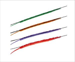
To explore the self-similarity of structure functions in the inner region under the impact of the over-tripped conditions, the even-order structure functions up to the tenth order are plotted in figure 3. The structure functions are normalized by the different characteristic scales, which are the Kolmogorov scales (Kolmogorov velocity ${u_K} = {(\nu \langle \varepsilon \rangle )^{1/4}}$ and Kolmogorov length $\eta = {({\nu ^3}/\langle \varepsilon \rangle )^{1/4}}$, where $\langle \varepsilon \rangle = 15\nu {(\partial u/\partial x)^2}$ is the estimate of the mean dissipation rate based on the local-homogeneity assumption) and the Taylor scales (the root mean square of the velocity fluctuations ${u_\lambda } = {\langle {u^2}\rangle ^{1/2}}$ and Taylor length scale $\lambda = {(15\nu u_\lambda ^2/\langle \varepsilon \rangle )^{1/2}}$). In figure 3, the line colour for each order structure function switching from dark to light represents an increase of the rod diameter from ${D_c} = 1$ to 20 mm in case III. In the plot, the higher-order structure functions are presented since they hold the information about internal intermittency (Landau & Lifshitz Reference Landau and Lifshitz1963), which represents a stochastic behaviour of very intense fluctuations with a higher frequency of occurrence than that predicted by a Gaussian distribution and occurs predominantly at the small scales. In the current study, with increasing tripping rod diameter, the large-scale structures generated by the tripping configurations are enhanced, which provides a modification effect on the small scales in the inner region (Mathis et al. Reference Mathis, Hutchins and Marusic2009; Baars et al. Reference Baars, Hutchins and Marusic2017; Marusic et al. Reference Marusic, Baars and Hutchins2017; Tang et al. Reference Tang, Jiang, Zhou and Lu2024). Thus, under the tripping influence in the over-tripped conditions, whether the similarity of the ISR could be established arouses our interest.

Figure 3. Distribution of even-order structure functions up to the tenth order at ${y^ + } \approx 80$ for various tripping conditions with different rod diameters in case III. The structure functions are normalized by (a) the Kolmogorov scales and (b) the Taylor scales. The line colour from light to dark corresponds to increasing tripping rod diameters from ${D_c} = 1$ to 20 mm in case III.

Figure 3 shows the even-order structure functions at the wall-normal location of ${y^ + } \approx 80$. In figure 3(a), for the second order, there is reasonable support for self-similarity for various tripping configurations, since an adequate collapse of structure functions can be observed almost over the entire r space. At the smallest scales, the collapse is perfect, which suggests the structure functions obey the classical Kolmogorov scaling $\langle {({\varDelta _r}u)^2}\rangle /u_K^2 \propto \; {(r/\eta )^2}$. At the largest scales, the self-similarity still holds with acceptable accuracy despite the tripping influence and finite-Reynolds-number effects. However, the situation is different for the higher-order structure functions. The self-similarity of structure functions is not strictly valid. Specifically, the eighth- and tenth-order structure functions normalized by the Kolmogorov scales (${u_K}$ and $\eta $) reveal a non-collapsing and clearly non-self-similar arrangement over the entire range of scales. In addition, as regards the performance of the Kolmogorov similarity at the smallest scales, it requires higher-resolution datasets for observation. Similarly, the structure functions do not satisfy the self-similarity over the entire scale range after normalization with the Taylor scales (figure 3b). As shown, except for the collapse at the intermediate scales, the Taylor scales lead to a certain discrepancy in the dissipative range and at the large scales on increasing the order. This finding confirms the general understanding of turbulence that the structure functions do not feature universality over the entire range of scales, specifically at low to moderate Reynolds numbers (Pearson & Antonia Reference Pearson and Antonia2001).

As indicated in the previous investigation (Landau & Lifshitz Reference Landau and Lifshitz1963), the non-universality of the higher-order structure functions is highly sensitive to different effects, such as internal intermittency and finite-Reynolds-number effects. Especially, in the current study, the generated large-scale wake structures by the over-tripped rods have amplitude and frequency modification effects on the small scales in the inner region, as presented in Appendix A. Both the amplitude and frequency modulation coefficients are increased with the tripping diameter, which means that generated large-scale structures could alter the internal intermittency behaviour based on modulation effects and result in the non-universality of the higher-order statistics, as shown in figure 3.

Figure 4 plots the comparison of the p.d.f.s of the velocity gradients $\partial u/\partial x$ at the wall-normal height ${y^ + } \approx 80$ for various tripping cases III-D1–D20. It shows that the p.d.f.s are non-Gaussian and have stretched exponential tails, which is very similar to the p.d.f.s in many other kinds of turbulent flows, such as isotropic turbulence (Gotoh, Fukayama & Nakano Reference Gotoh, Fukayama and Nakano2002) and turbulent jet flows (Gauding et al. Reference Gauding, Bode, Brahami, Varea and Danaila2021). On increasing the tripping rod diameter, the p.d.f.s have almost a consistent distribution. Careful observation shows that the tails of the p.d.f.s become slightly stretched in the over-tripped cases, which should be related to the footprint of large-scale wake structures generated by the tripping condition with increasing rod diameter (the evidence of the footprint effect of large scales in the near-wall region is exhibited in Appendix B).

Figure 4. Comparison of p.d.f.s of velocity gradients at ${y^ + } \approx 80$ for various tripping conditions with different rod diameters in cases III-D1–D20. The black dashed line indicates a normal distribution. The curves are normalized by the standard deviation ${\langle {(\partial u/\partial x)^2}\rangle ^{1/2}}$.

3.2. Relative relations of structure functions for the ECR scales

In the spirit of the ESS hypothesis, the relation of the velocity structure functions as expressed in (1.4) for the ECR scales is examined to further explore universality in this part. Following the previous work from de Silva et al. (Reference de Silva, Krug, Lohse and Marusic2017), figure 5 plots the relation of ${\langle {({\varDelta _r}{u_ + })^{2p}}\rangle ^{1/p}}$ versus $\langle {({\varDelta _r}{u_ + })^2}\rangle$ at ${y^ + } \approx 80$ for all the cases III-D1–D20. All the results are computed at a fixed wall-normal location of ${y^ + } \approx 80$, similar to that processed in figures 3 and 4. In the plot, the tenth-order $(2p = 10)$ structure function is also involved to highlight any subtle differences in the ESS framework. In figure 5, the distributions of ${\langle {({\varDelta _r}{u_ + })^{2p}}\rangle ^{1/p}}$ versus $\langle {({\varDelta _r}{u_ + })^2}\rangle$ for almost all the scales are shown by the coloured lines, from which the ESS scaling cannot be extracted directly, as shown by de Silva et al. (Reference de Silva, Krug, Lohse and Marusic2017). However, for the ECR-scale range of $y < r < \delta $, as marked by the symbols, the results obviously reveal a convincingly extended range of scaling behaviour in the ESS-inspired framework. The results show a good collapse of the higher-order moments up to $2p = 10$ and provide direct support for the investigation of de Silva et al. (Reference de Silva, Krug, Lohse and Marusic2017). Furthermore, the current study extends the application of the ECR-scale similarity to the over-stimulated boundary layers, which are in an adaptation region to recover from the leading-edge tripping effects and return to the canonical state. The good agreement for each higher order $2p = 4,\;6,\;8,\;10$ in figure 5 suggests that the scaling behaviour of ECR scales is independent of the current tripping influence.

Figure 5. The ESS plot for higher-order moments for the same databases shown in figures 3 and 4. The results are computed at the wall-normal location of ${y^ + } \approx 80$; ${\langle {({\varDelta _r}{u_ + })^{2p}}\rangle ^{1/p}}$ versus $\langle {({\varDelta _r}{u_ + })^2}\rangle $: (a) $p = 2$, (b) $p = 3$, (c) $p = 4$, (d) $p = 5$, as shown in the coloured lines for almost the entire scale range of r. The data in the ECR-scale range of $y < r < \delta $ are shown by the symbols. The solid black lines (——) correspond to a fit following (1.4) in the ECR-scale range at case III-D20.

The extended range of scaling behaviour in figure 5 provides an opportunity to have a reliable estimation of the scaling coefficients (slopes ${D_p}/{D_1}$, $p = 2,\;3,\;4,\;5$). To further quantify the relation, the ratios of ${D_p}/{D_1}$ are computed based on a linear fit in the ECR-scale range $y < r < \delta $. The work of de Silva et al. (Reference de Silva, Krug, Lohse and Marusic2017) utilized this procedure to exhibit a good description of the ECR-scale similarity at $R{e_\tau } \approx 900$, which indicates that ECR scaling coefficients can be confidently estimated from databases at low Reynolds numbers when no clear logarithmic region exists. The current study confirms the scaling universality of ECR scales based on the datasets in the range of $R{e_\tau } \approx 500{-}3500$, especially under the tripping influence. Figure 6 shows the estimates of the higher-order slope ratios ${D_p}/{D_1}$ over a range of ECR scales for various tripping rods with different diameters. We can note that the coefficient ratio ${D_p}/{D_1}$ holds a consistent distribution for all the tripping cases. For comparison, the results in the inner region of TBL flow ($\kern 1.8pt {y^ + } \approx 150$, $R{e_\tau } \approx 1600$) by Sillero, Jiménez & Moser (Reference Sillero, Jiménez and Moser2013) are also shown in the plot. As shown, ${D_p}/{D_1}$ in the current study is in accordance with the result by Sillero et al. (Reference Sillero, Jiménez and Moser2013). The consistent scaling behaviour confirms that the relation of the structure functions in the ECR scales is independent of the different tripping conditions in the current study.

Figure 6. Distribution of ratios ${D_p}/{D_1}$ versus p, from the relation in figure 5. The symbol of the blue circle represents the results of TBL DNS datasets ($\kern 1.8pt {y^ + } \approx 150$, $R{e_\tau } \approx 1600$) from Sillero et al. (Reference Sillero, Jiménez and Moser2013).

Furthermore, to explore the performance of the structure functions for the ECR scales at a broader wall-normal extent, figure 7 plots the distribution of ratios ${{D_p}/{D_1}}{(p = 2,3,4,5)}$ across the entire boundary layer for all the tripping cases. Similar to figure 6, the coefficient ratio calculated from the direct numerical simulation (DNS) TBL datasets by Sillero et al. (Reference Sillero, Jiménez and Moser2013) ($\kern 1.8pt {y^ + } \approx 150$, $R{e_\tau } \approx 1600$) is employed for comparison (black lines). As shown, a good collapse of the ratio is noted in the inner region for the various tripping conditions, which indicates that the scaling universality of the ECR scales is independent of the tripping rod diameter. Meanwhile, the values of ${D_p}/{D_1}$ in the inner region appear unchanged. This constant of ${D_p}/{D_1}$ is consistent with the suggestions by de Silva et al. (Reference de Silva, Krug, Lohse and Marusic2017) in the log region of high-Reynolds-number TBLs. In addition, based on the ESS-inspired framework, the universality of the scaling of the ECR scales extends beyond the logarithmic region of the boundary layer. From the insets in figure 7, it can be seen that the universality extends almost up to $y/\delta \approx 0.5$ for all the tripping cases. Since the boundary-layer thickness is increased with the tripping diameter, it can be deduced that a further reaching universality is performed by increasing the tripping rod diameter.

Figure 7. Distribution of ratios ${D_p}/{D_1}$ along the wall-normal heights of $\kern 1.8pt {y^ + }$ ($\kern 0.06em y/\delta $ in the insets) for all the tripping cases III-D1–D20; (a) $p = 2$, (b) $p = 3$, (c) $p = 4$ and (d) $p = 5$. The coefficient ratio value calculated from the TBL DNS datasets (${z^ + } \approx 150$, $R{e_\tau } \approx 1600$) from Sillero et al. (Reference Sillero, Jiménez and Moser2013) is also plotted in black lines for comparison. The results of ratios ${D_p}/{D_1}$ for cases I and II are shown in Appendix C.

From these findings, it can be concluded that, even though the tripping impacts are likely to be embodied in structure functions at different orders, as shown in figures 3 and 4, we are able to exhibit the similarity of ECR scales by accurately quantifying the universal scaling of the ratios between two structure functions (${D_p}/{D_1}$) over a much larger wall-normal extent. Analogously, recent work on high-order moments (Yang et al. Reference Yang, Marusic and Meneveau2016a,Reference Yang, Meneveau, Marusic and Biferaleb; Xia et al. Reference Xia, Brethouwer and Chen2018) also indicated that the extent of logarithmic scaling as a function of y increases when examining ratios between moment functions in ESS form. The observation of the ESS region could be attributed to the argument that the bulk flow or viscous effects have a similar action on the structure function for the ECR scales (Yang et al. Reference Yang, Marusic and Meneveau2016a,Reference Yang, Meneveau, Marusic and Biferaleb), which can be further extended under the over-tripped conditions.

Additionally, the relative relation of structure functions in (1.4) is challenged in the outer part around the edge of the boundary layer. This region is dominated by the turbulent/non-turbulent intermittency, rather than the ECR scales following Townsend's attached hypothesis. Hence, it is reasonable to note an obvious discrepancy in the examination of the scaling for ECR scales in the ESS framework, as shown in figure 7. In the following, the similarity behaviour in the outer region will be examined by considering the external intermittency.

4.1. The external intermittency

The external intermittency is described as the flow alternating between turbulent and substantially irrotational non-turbulent motions in the outer-layer region (Corrsin & Kistler Reference Corrsin and Kistler1955; Townsend Reference Townsend1976). The turbulent region and non-turbulent region are separated by the turbulent/non-turbulent interface (TNTI), which is assumed to be a sharp and highly contorted superlayer (Bisset, Hunt & Rogers Reference Bisset, Hunt and Rogers2002; Chauhan et al. Reference Chauhan, Philip, de Silva, Hutchins and Marusic2014; da Silva et al. Reference da Silva, Hunt, Eames and Westerweel2014; Philip et al. Reference Philip, Meneveau, de Silva and Marusic2014). The mean intermittency distribution is argued to be independent of Reynolds number (Fiedler & Head Reference Fiedler and Head1966). In the artificially thickened boundary-layer flows, the generated wake structures from the leading-edge trips can provide a remarkable alteration to the external intermittency in the adaptive region (Rodríguez-López et al. Reference Rodríguez-López, Bruce and Buxton2016a; Buxton et al. Reference Buxton, Ewenz Rocher and Rodríguez-López2018; Tang et al. Reference Tang, Jiang, Zhou and Lu2024), by inquiring into the statistics of the outer-layer region, such as mean velocity, variance, energy spectra and high-order statistics.

To observe the external intermittency behaviour, it is necessary to detect the TNTI, which is a continuous ongoing research activity in turbulent flows. Several detecting methods have also been proposed for the experimental datasets, by considering that the intrinsic background turbulence in free stream. For particle image velocimetry measurements, the TNTI was detected by the technique based on turbulent kinetic energy (Chauhan et al. Reference Chauhan, Philip, de Silva, Hutchins and Marusic2014), local homogeneity (Reuther & Kähler Reference Reuther and Kähler2018), fuzzy clustering of the streamwise velocity field (Fan et al. Reference Fan, Xu, Yao and Hickey2019; Younes et al. Reference Younes, Gibeau, Ghaemi and Hickey2021), track of the Lagrangian particle trajectories (Long, Wu & Wang Reference Long, Wu and Wang2021) and so on. For the current one-dimensional flow data by hot-wire measurement, the detection of intermittency relies upon identifying whether the probe is measuring turbulent or non-turbulent fluids. Therefore, a turbulent kinematic energy criterion proposed by Chauhan et al. (Reference Chauhan, Philip, de Silva, Hutchins and Marusic2014) is utilized to detect the TNTI in this study. This procedure has been extensively used in recent works (de Silva et al. Reference de Silva, Philip, Chauhan, Meneveau and Marusic2013; Chauhan et al. Reference Chauhan, Philip, de Silva, Hutchins and Marusic2014; Kwon, Hutchins & Monty Reference Kwon, Hutchins and Monty2016; Saxton-Fox & McKeon Reference Saxton-Fox and McKeon2017; Buxton et al. Reference Buxton, Ewenz Rocher and Rodríguez-López2018; Chen et al. Reference Chen, Fan, Tang, Wang, Shi and Jiang2023), and only a brief description will be given here.

The intermittency interface detector function is introduced to evaluate the external intermittency, which is defined as

(4.1)\begin{equation}\varphi (i) = \frac{{100}}{{U_\infty ^2}}\frac{1}{3}\sum\limits_{j ={-} 1}^1 {{{({u_{i + j}} - {U_\infty })}^2}} ,\end{equation}

where the index i is an arbitrary instant in the temporal domain and the summation over index j indicates a mean over three consecutive measurements in a time series. The turbulent (non-turbulent) fluids can be detected as those for which $\varphi (i)$ is higher (lower) than a given threshold ${\varphi _{th}}$. A binary representation of the flow is obtained using the threshold, and the binary representation is considered as

(4.2)\begin{equation}\psi (i) = H(\varphi (i) - {\varphi _{th}}) = \left\{ {\begin{array}{@{}cc@{}} {1,}&{\varphi (i) \ge {\varphi_{th}}}\\ {0,}&{\varphi (i) < {\varphi_{th}}} \end{array}} \right., \end{equation}

where H is the Heaviside function and $\psi (i)$ is the so-called intermittency function. Then, as proposed by Klebanoff (Reference Klebanoff1955), an intermittency parameter $\gamma (y)$ at the wall-normal location of y is defined as

(4.3)\begin{equation}\gamma (y) = \frac{1}{N}\sum\limits_{i = 1}^N {\psi (i,y)} ,\end{equation}

which quantifies the proportion of time that the flow is turbulent. Close to the wall, the flow is expected to be fully turbulent, $\gamma (y) = 1$, the non-turbulent fluids gradually have more occurrence far away from the wall, and $\gamma (y) = 0$ in the free stream. It is well known that the intermittency profile of $\gamma (y)$ in the TBL can be described by the error function (Corrsin & Kistler Reference Corrsin and Kistler1955; Klebanoff Reference Klebanoff1955; Fiedler & Head Reference Fiedler and Head1966; Hedleyt & Keffer Reference Hedleyt and Keffer1974)

(4.4)\begin{equation}\gamma (y) = \frac{1}{{{\sigma _I}\sqrt {2{\rm \pi} } }}\int_y^\infty {\textrm{exp}\left( { - \frac{{{{(y - {Y_I})}^2}}}{{2\sigma_I^2}}} \right)\textrm{d}y} ,\end{equation}

here, ${Y_I}$ is the wall-normal location of the mean interface where $\gamma ({Y_I}) = 0.5$ and ${\sigma _I}$ is the standard deviation of the instantaneous interface position ${y_I}$ relative to the mean position ${Y_I}$. Here, ${Y_I}$ and ${\sigma _I}$ are the estimated parameters by fitting the measurement intermittency profile to the function of (4.4). From the above procedure, it can be seen that the intermittency is dependent on the given threshold value ${\varphi _{th}}$, which is related to the values of ${Y_I}$ and ${\sigma _I}$. Thus, by fitting the error function in (4.4), a threshold of 0.07–0.08 is chosen to calculate the intermittency profile $\gamma (y)$ for all the cases in the current study. The wall-normal intermittency profiles $\gamma (y)$ in the outer scaling $y/\delta $ are shown in figure 8. As shown, $\gamma (y)$ exhibits a normal distribution for all the tripping conditions in the current study, by presenting good fittings to the error function in (4.4). Considering that the current tripping conditions make a significant alteration to the flow fields in the wake region, this could challenge the fit precision based on the wake function in determining the ‘true’ boundary-layer thickness (the wall distance where $\bar{U} = {U_\infty }$ exactly) (Chauhan et al. Reference Chauhan, Monkewitz and Nagib2009). Thus, the conventional boundary-layer thickness ($\kern 1.8pt y = \delta $ where $\bar{U}/{U_\infty } = 0.99$) is used in this study, which is smaller than the ‘true’ boundary-layer thickness (Chauhan et al. Reference Chauhan, Monkewitz and Nagib2009). As shown in figure 8, $\gamma \approx 0.2{-}0.4$ (increase with ${D_c}$) at $y/\delta = 1$ in all cases, which is consistent with the previous investigations (Kovasznay, Kibens & Blackwelder Reference Kovasznay, Kibens and Blackwelder1970; Hedleyt & Keffer Reference Hedleyt and Keffer1974; Chen & Blackwelder Reference Chen and Blackwelder1978; Chauhan et al. Reference Chauhan, Philip, de Silva, Hutchins and Marusic2014). The standard deviation ${\sigma _\gamma }$ of the interface location is presented as a function of the tripping rod diameter in figure 9. The solid line indicates the range of ${\sigma _\gamma } \approx 0.15{-}0.18$, which is obtained from the data of canonical TBL flows (Corrsin & Kistler Reference Corrsin and Kistler1955; Hedleyt & Keffer Reference Hedleyt and Keffer1974). It shows that ${\sigma _\gamma }$ has a good agreement with the results in the moderately tripped cases. Then, increasing ${D_c}$ alters the intermittent region by introducing strong perturbations. The intermittency region rapidly extends further away from the wall by holding a wider proportion in the boundary layer, as shown in figure 8, thus, an increased ${\sigma _\gamma }$ is noted in figure 9.

Figure 8. Intermittency parameter profile $\gamma (y)$ as a function of $y/\delta $ in outer scaling for different tripping rod diameters with different free-stream velocities; (a) case I, (b) case II, (c) case III. Coloured lines represent the result by fitting (y) to the error function in (4.4).

Figure 9. Standard deviation of the interface location ${\sigma _\gamma }$ as a function of tripping rod diameter ${D_c}$ for the cases I, II and III. Solid line represents the range of ${\sigma _\gamma } \approx 0.15{-}0.18$.

With this definition of the intermittency parameter $\gamma $, any conventionally averaged quantity $\langle \phi \rangle $ can be decomposed as

(4.5)\begin{equation}\langle \phi \rangle = \gamma {\langle \phi \rangle _T} + (1 - \gamma ){\langle \phi \rangle _N},\end{equation}

where ${\langle \phi \rangle _T}$ and ${\langle \phi \rangle _N}$ indicate the conditional averaging results by only considering either turbulent or non-turbulent regimes (Mellado, Wang & Peters Reference Mellado, Wang and Peters2009; Gauding et al. Reference Gauding, Bode, Brahami, Varea and Danaila2021). The conditional averages are defined with the binary indicator function, $\psi $, as

(4.6)\begin{equation}{\langle \phi \rangle _T} = \langle \psi \phi \rangle , \end{equation}

and

(4.7)\begin{equation}{\langle \phi \rangle _N} = \langle (1 - \psi )\phi \rangle .\end{equation}

4.2. Intermittency structure function

Referring to the external intermittency, when we calculate the statistical moments of the velocity increments of two points separated by a spatial distance r, different conditions should be considered: (I) both points are located within the turbulent regime, (II) both points are within the non-turbulent regime and (III) one point in the turbulent regime and the other one in the non-turbulent regime. For locally homogeneous turbulence, the corresponding probabilities for the different conditions can be obtained as ${\gamma _{TT}} = \gamma - {\textstyle{1 \over 2}}{\varTheta _I}$, ${\gamma _{NN}} = 1 - \gamma - {\textstyle{1 \over 2}}{\varTheta _I}$ and ${\gamma _{TN}} = {\varTheta _I}$, where ${\varTheta _I} = \langle {(\psi (x + r) - \psi (x))^2}\rangle $ is known as the intermittency structure function (Kuznetsov, Praskovsky & Sabelnikov Reference Kuznetsov, Praskovsky and Sabelnikov1992). It is clear that ${\gamma _{TT}} + {\gamma _{NN}} + {\gamma _{TN}} = 1$. From the probabilities in different conditions, it can be deduced that the ratio

(4.8)\begin{equation}\frac{{{\gamma _{TT}}}}{\gamma } = 1 - \frac{{{\varTheta _I}}}{\gamma },\end{equation}

which represents the conditional probability that one point of the velocity increment is in the turbulent regime considering that the other point is also in the turbulent regime. From the above equations, it can be deduced that ${\gamma _{TT}}/\gamma \to 1$ (${\gamma _{TT}} \to \gamma $) as ${\varTheta _I} \to 0$ if $r \to 0$. Figure 10 shows ${\gamma _{TT}}/\gamma $ against spatial distance $r/\eta $ at different wall-normal positions the intermittency of which is in the range of $\gamma = 0.1{-}0.9$ for case III-D20 as a representative case. It is expected that in the inner region with the higher value $\gamma \to 0.9$, ${\gamma _{TT}}/\gamma $ is close to unity with $r \to 0$ and has a relatively slowly decreasing trend with increasing separation distance r. Further away from the wall, ${\gamma _{TT}}/\gamma $ decreases remarkably at larger r. A similar distribution was reported in the turbulent jet flow by Gauding et al. (Reference Gauding, Bode, Brahami, Varea and Danaila2021). Due to the external intermittency of the alternation between turbulent and non-turbulent fluid and the decreased proportion of turbulent excursion, it is reasonable to have lower ${\gamma _{TT}}/\gamma $ toward the edge of the boundary layer ($\gamma \to 0.1$) at the larger-separation distance.

Figure 10. Conditional probability ${\gamma _{TT}}/\gamma $ against spatial distance, $r/\eta $, at different wall-normal positions with the intermittency parameter in the range of $\gamma = 0.1{-}0.9$ for case III-D20.

To further explore the feature of the intermittency function $\psi $, one-dimensional random telegraphic signals ${\psi _{ts}}$ are introduced, which have randomly distributed values of ${\psi _{ts}} = 1$ in turbulent regimes and ${\psi _{ts}} = 0$ in non-turbulent regimes, with the corresponding probabilities of $P({\psi _{ts}} = 1) = {\gamma _{ts}}$ and $P({\psi _{ts}} = 0) = 1 - {\gamma _{ts}}$. The second-order moment of the increment ${\varTheta _{I,ts}}(r)$ can be expressed by the autocorrelation function of ${\psi _{ts}}$, as

(4.9)\begin{equation}{\varTheta _{I,ts}}(r) = \langle {({\psi _{ts}}(x + r) - {\psi _{ts}}(x))^2}\rangle = 2({R_{{\psi _{ts}}}}(0) - {R_{{\psi _{ts}}}}(r)) = 2({\gamma _{ts}} - {R_{{\psi _{ts}}}}),\end{equation}

where ${R_{{\psi _{ts}}}}(r)$ represents the analytical expression of the autocorrelation of ${\psi _{ts}}$, which is expressed as (Machlup Reference Machlup1954; Fitzhugh Reference Fitzhugh1983; Thiesset et al. Reference Thiesset, Duret, Ménard, Dumouchel, Reveillon and Demoulin2020)

(4.10)\begin{equation}{R_{{\psi _{ts}}}}(r) = \langle {\psi _{ts}}(x + r){\psi _{ts}}(x)\rangle = {\gamma _{ts}}({\gamma _{ts}} + (1 - {\gamma _{ts}})\,{\textrm{e}^{ - r/{\mathcal{L}_{ts}}}}).\end{equation}

In (4.10), ${\mathcal{L}_{ts}}$ is a characteristic length scale, ${\mathcal{L}_{ts}} = 2{\gamma _{ts}}(1 - {\gamma _{ts}}){[{\lim _{r \to 0}}({\varTheta _{I,ts}}(r)/r)]^{ - 1}}$, that relates to the probability of ${\psi _{ts}}$ transiting from a value of 1 to 0 and vice versa (Machlup Reference Machlup1954; Fitzhugh Reference Fitzhugh1983; Thiesset et al. Reference Thiesset, Duret, Ménard, Dumouchel, Reveillon and Demoulin2020).

From the expression of (4.9) and (4.10), an analytical intermittency structure function of the random telegraphic signal can be expressed as

(4.11)\begin{equation}{\varTheta _{I,ts}}(r) = 2{\gamma _{ts}}(1 - {\gamma _{ts}})(1 - {\textrm{e}^{ - r/{\mathcal{L}_{ts}}}}).\end{equation}

From (4.11), it can be seen that, at large separations, ${\varTheta _{I,ts}}(r \to \infty ) = 2{\gamma _{ts}}(1 - {\gamma _{ts}})$, and for the small-separation limit it can be deduced that

(4.12)\begin{equation}\mathop {\lim }\limits_{r \to 0} {\varTheta _{I,ts}}(r) = 2{\gamma _{ts}}(1 - {\gamma _{ts}})\frac{r}{{{\mathcal{L}_{ts}}}} + {\rm O}({r^2}),\end{equation}

which indicates that ${\varTheta _{I,ts}}(r)$ is proportional to r when the separation distance r is small compared with ${\mathcal{L}_{ts}}$.

Then, we can compare the analytical intermittency structure function of the random telegraphic signal, ${\varTheta _{I,ts}}$, with the intermittency structure function ${\varTheta _I}$ of the wall turbulence signals for case III-20 in the current study. In figure 11, the intermittency structure function ${\varTheta _I}$ is presented for the different wall-normal positions, which is normalized by the large-scale limit $2\gamma (1 - \gamma )$. The separation distance r is normalized by the characteristic length scale $\mathcal{L}$. The plot shows a good collapse between ${\varTheta _{I,ts}}/2{\gamma _{ts}} (1 - {\gamma _{ts}})$ and ${\varTheta _I}/2\gamma (1 - \gamma )$ at the scales of the small- and large-scale limits. A clear discrepancy is noted in the intermediate-scale range, which becomes more obvious as increasing wall-normal heights (decreasing intermittency parameter $\gamma $). This discrepancy was also reported in the intermittent range scales of turbulent jet flows (Gauding et al. Reference Gauding, Bode, Brahami, Varea and Danaila2021) and liquid–gas turbulence (Thiesset et al. Reference Thiesset, Duret, Ménard, Dumouchel, Reveillon and Demoulin2020). In fact, the TNTI is widely argued to be a self-similar fractal which can be quantified by the fractal dimension (Sreenivasan & Meneveau Reference Sreenivasan and Meneveau1986). The self-similar fractal behaviour has been confirmed in different classes of flows, such as boundary layer, jet flow, plane wake and mixing layer (Sreenivasan & Meneveau Reference Sreenivasan and Meneveau1986; Meneveau & Sreenivasan Reference Meneveau and Sreenivasan1991). Furthermore, Tang et al. (Reference Tang, Jiang, Zhou and Lu2024) confirmed that, under the impact of the tripping conditions in the current study, the boundary-layer flows remain self-similar fractals with identical fractal dimensions. Thus, the discrepancy in the intermediate-scale range in figure 11 is due to the fact that the morphology of the TNTI is not fully random but instead characterized by the self-similar fractal behaviour of turbulence.

Figure 11. Comparison of the intermittency structure function ${\varTheta _I}$ (coloured lines) at different wall-normal positions ($\gamma = 0.1{-}0.9$) with the analytical intermittency structure function of the random telegraphic signal (${\varTheta _{I,ts}}$, blue dashed lines). The black dashed lines indicate the analytical small- and large-scale limits. Data for case III-D20.

As mentioned earlier, the characteristic length scale $\mathcal{L}$ relates to the transiting probability of $\psi $, which is equivalent to the jump frequency transiting from a value of 1 to 0 and vice versa. The jump frequency is expressed as

(4.13)\begin{equation}{f_\psi } = \left\langle {\left|{\frac{{\partial \psi }}{{\partial x}}} \right|} \right\rangle = \frac{{{n_I}}}{{{\mathcal{L}_0}}},\end{equation}

where ${f_\psi }$ represents the number of turbulent/non-turbulent (non-turbulent/turbulent) transitions ${n_I}$ per length in the streamwise direction. Following the previous investigations (Debye, Anderson & Brumberger Reference Debye, Anderson and Brumberger1957; Thiesset et al. Reference Thiesset, Duret, Ménard, Dumouchel, Reveillon and Demoulin2020; Gauding et al. Reference Gauding, Bode, Brahami, Varea and Danaila2021), it can be deduced that ${\lim _{r \to 0}}({\varTheta _I}/r) = \langle |\partial \psi /\partial x|\rangle$ from the small-separation limit in (4.12), which means that the small-separation limit of the second-order structure function is equal to the jump frequency. Figure 12(a) shows the jump frequency ${f_\psi }$ as a function of the wall-normal heights for all the cases III-D1–D20. In the plot, ${f_\psi }$ has a clear maximum for each tripping configuration, which means that the alteration between turbulent and non-turbulent happens most frequently. On increasing the tripping rod diameter, the maximum ${f_\psi }$ moves outwards with a gradually decreasing trend, meanwhile, the wall-normal span of ${f_\psi }$ has a broader extent, which implies a growing wall-normal extent of the TNTI in the over-tripped conditions. This is consistent with the results of the intermittency parameters in figure 8. It is shown that, with increasing tripping rod diameter, the intermittency region rapidly extends further away from the wall by holding a wider proportion of the boundary layer (as shown in the inset of figure 12a). Specifically, the intermittency parameter exhibits a normal distribution with an increasing standard deviation ${\sigma _\gamma }$. Here, ${\sigma _\gamma }$ is suggested to be a measure of the width of the intermittent zone. Thus, ${\sigma _\gamma }$ is employed for the normalization in figure 12(b), and ${f_\psi }$ exhibits a self-preserving shape with intermittent factor in the relationship of ${f_\psi }{\sigma _\gamma } \propto \gamma $. This finding is consistent with the growth of the characteristic length scale of TNTI with increasing tripping diameter in the framework of self-similar behaviour.

Figure 12. (a) Jump frequency ${f_\psi }$ as a function of the wall-normal height ${y^ + }$ ($\kern 1.8pt y/\delta $ in the inset), (b) self-preservation of ${f_\psi }$ after normalization with the standard deviation of intermittent parameter ${\sigma _\gamma }$, as a function of $\gamma $. The data are for the various tripping conditions with different rod diameters (cases III-D1–D20). The results of cases I and II are shown in Appendix D.

4.3. Structure functions and the effects of external intermittency

The current tripping configurations provide a predominant influence on the intermittency in the wake region, such as the jump frequency, which attracts our interest as to whether the self-similarity of the structure functions can be observed in the intermittent zone. Figure 13 shows the normalized even-order structure functions up to the tenth order at the different wall-normal heights for the case III-D20. As shown in figure 13(a,b), the structure functions are normalized by the Kolmogorov scales (${u_K}$ and $\eta $) and the Taylor scales (${u_\lambda }$ and $\lambda $), respectively, similar to figure 3. It seems that the second order shows the self-similarity as regards the wall-normal heights in the range of $\gamma = 0.1{-}0.9$, by showing an acceptable collapse in either form of the normalizations. The remarkable collapse is noted at the small scales; the distribution can be explained by the validation of classical Kolmogorov scaling. At the large scales, a certain discrepancy is noted in the Kolmogorov-scale normalizations, which should be attributed to the external intermittency in the over-tripped conditions. It is evident that the higher-order structure functions (fourth to tenth order) exhibit a clearly non-collapsing and non-self-similar arrangement over the entire range of scales through the intermittent zone. This result is expected in higher-order statistics, which are very sensitive to various factors, especially external intermittency, and probably promoted under the influence of the tripping conditions. Additionally, by comparing with the results in the inner region, as shown in figure 3(a), it is indicated that the spatial resolution effect of the hot-wire probe on the estimation of the Kolmogorov length scale should be neglected from the reasons causing the non-collapsing distribution in figure 13(a).

Figure 13. Distribution of even-order structure functions up to the tenth order at different wall-normal heights in the range of $\gamma = 0.1{-}0.9$ for case III-D20. The structure functions are normalized by (a) the Kolmogorov scales and (b) the Taylor scales, as similar in figure 3. The line colour from dark to light means that the wall-normal position moves outwards, corresponding to an intermittency parameter from $\gamma = 0.9$ to 0.1.

To reveal the cause behind the lack of self-similarity of higher-order structure functions, we present the characteristics of intermittency. Following Batchelor & Townsend (Reference Batchelor and Townsend1949), the turbulent signals are intermittent when the fine structure of the turbulence tends to be locally concentrated, intermittent in nature and randomly scattered through the fluid in a spotty way. This spatially spotty pattern becomes more prominent with increasing order of the velocity derivative. Hence, the higher-order moment of velocity derivative is a suitable tool to probe turbulent intermittency, and the flatness is defined as

(4.14)\begin{equation}F = \frac{{{{\left\langle {\left( {\dfrac{{\partial u}}{{\partial x}}} \right)}^4 \right\rangle }}}}{{{{\left\langle {\left( {\dfrac{{\partial u}}{{\partial x}}} \right)}^2\right\rangle }}^2}},\end{equation}

which is widely accepted to represent intermittency at the fine scales. Note that, for the velocity increment ${\varDelta _r}u = u(x + r) - u(x)$, when $r \to 0$, ${\varDelta _r}u$ at small scales is essentially equivalent to the derivative.

For the purpose of testing the original Kolmogorov similarity hypothesis, the evolution of high-order statistics of the velocity derivatives with $R{e_\lambda }$ has been widely examined. It was indicated that the statistic of F is affected by two factors, which are the finite-Reynolds-number effect and the flow conditions (Antonia et al. Reference Antonia, Tang, Djenidi and Danaila2015, Reference Antonia, Djenidi, Danaila and Tang2017; Djenidi et al. Reference Djenidi, Antonia, Talluru and Abe2017; Meldi, Djenidi & Antonia Reference Meldi, Djenidi and Antonia2018; Tang et al. Reference Tang, Antonia, Djenidi, Danaila and Zhou2018). Figure 14(a) shows the distribution of the flatness factor F against $R{e_\lambda }$ for all the data with the intermittency parameter in the range of $\gamma = 0.1{-}0.9$ (for cases III-D1–D20). In the plot, with increasing tripping diameter ${D_c}$, both F and $R{e_\lambda }$ exhibit a broader extent. Each of the tripping conditions indicates that the flatness factor of the velocity derivative F is increased on reducing $R{e_\lambda }$ (also $\gamma $). From the numerous investigations, the $R{e_\lambda }$ dependence of F in a fitting power law has been sought empirically in different kinds of flows, and the fitting power law $F\sim (1.14 \mp 0.19)Re_\lambda ^{0.34 \pm 0.03}$ was derived from an abundance of turbulent data (Antonia, Satyaprakash, & Hussain Reference Antonia, Satyaprakash and Hussain1982; Jiménez et al. Reference Jiménez, Wray, Saffman and Rogallo1993; Wang et al. Reference Wang, Chen, Brasseur and Wyngaard1996; Sreenivasan & Antonia Reference Sreenivasan and Antonia1997; Gotoh et al. Reference Gotoh, Fukayama and Nakano2002; Ishihara et al. Reference Ishihara, Kaneda, Yokokawa, Itakura and Uno2007; Ishihara, Gotoh & Kaneda Reference Ishihara, Gotoh and Kaneda2009). The fitting power law is drawn in figure 14(a) for comparison. It can be seen that, at a high intermittent factor ($\gamma \to 0.9$), F shows a good collapse with the power law of $R{e_\lambda }$. The collapse means that the high-order statistics of fine-scale structures in the wall-normal region with the higher $\gamma $ are almost independent of the impact of external intermittency. The results are supported by Djenidi et al. (Reference Djenidi, Antonia, Talluru and Abe2017) that a constant flatness factor can be noted in the region $0.3 \le y/\delta \le 0.6$ (corresponding to high $\gamma $), in which both F and $R{e_\lambda }$ are independent of the distance to the wall. On decreasing the intermittent factor (further away from the wall), F has an obvious deviation from the fitting power law of $R{e_\lambda }$ by showing significantly greater values in figure 14(a), which could be attributed to the effect of the flow conditions of external intermittency. Similarly, figure 14(b) shows the dependence of F on the external intermittency parameter $\gamma $. As shown, F increases from an inner value close to 6 ($\gamma \to 0.9$) to a value around 50 ($\gamma \to 0.1$) close to the edge of the boundary layer. Considering that the velocity derivative can emphasize the fine-scale components but not cut out the low-frequency (large-scale) parts of the signal (Kuo & Corrsin Reference Kuo and Corrsin1971), the dependence of F confirms that the fine scales do not decouple from the large scales under the tripping effects and further supports that the external intermittency has a dominant impact on the fine scales. In fact, the remarkable change of F was also discussed by Gauding et al. (Reference Gauding, Bode, Brahami, Varea and Danaila2021) in turbulent jet flows. They linked the change of F to the local kinematics of TNTI by considering the non-equilibrium in the energy cascade and the direction of the inter-scale transport (Watanabe, da Silva & Nagata Reference Watanabe, da Silva and Nagata2019, Reference Watanabe, da Silva and Nagata2020), which is probably further promoted in the current over-tripped conditions.

Figure 14. Flatness factor of the velocity gradients F as a function of (a) Reynolds number $R{e_\lambda }$ (light to dark red colour represents an increase of intermittent parameter from $\gamma = 0.1$ to 0.9, the black line indicates the power law $F = (1.14 \mp 0.19)Re_\lambda ^{0.34 \pm 0.03}$) and (b) the intermittency parameter $\gamma $ (the line colour indicates the tripping rod diameter, ${D_c}$).

To further understand the impact of external intermittency, the conditional flatness factor of the velocity derivatives is defined as (following the expression of (4.6))

(4.15)\begin{equation}{F_T} = \frac{{\left\langle {\psi {{\left( {\dfrac{{\partial u}}{{\partial x}}} \right)}^4}} \right\rangle }}{{{{\left\langle {\psi {{\left( {\dfrac{{\partial u}}{{\partial x}}} \right)}^2}} \right\rangle }^2}}}.\end{equation}

The binary indicator function of intermittency $\psi $ is introduced to consider only the turbulent portion of the outer-layer flow. Figure 15(a,b) shows the distribution of conditional flatness factor ${F_T}$ against $R{e_\lambda }$ and $\gamma $, respectively. In figure 15(a), ${F_T}$ and $R{e_\lambda }$ show a good agreement with the power law ${F_T} = (1.14 \mp 0.19)Re_\lambda ^{0.34 \pm 0.03}$ for all the data at different wall-normal heights through the intermittent region. It is clear that the effect of the external intermittency, which leads to the obvious deviation (significantly high values of F in figure 14a), is excluded by examining the conditional flatness factor ${F_T}$, which is further confirmed by the distribution of the p.d.f.s of the velocity derivatives in figure 16. The power-law dependence of ${F_T}$ on $R{e_\lambda }$ in figure 15(a) implies that, in the turbulent regimes of the outer layer, the large-scale fluctuations play a role in determining the turbulence intermittency, the level of which increases with $R{e_\lambda }$ (Batchelor & Townsend Reference Batchelor and Townsend1949).

Figure 15. Conditional flatness factor of the velocity gradients ${F_T}$ as a function of (a) Reynolds number $R{e_\lambda }$ and (b) the intermittency parameter $\gamma $. Note that the presentation is completely consistent with that in figure 14 for comparison.

Figure 16. Conventional (a) and conditional (b) p.d.f.s of the velocity derivatives at different wall-normal positions as indicated in the legend of intermittent factor $\gamma $. The black dashed line indicates a normal distribution. The curves are normalized by the standard deviation $\sigma = {\langle {(\partial u/\partial x)^2}\rangle ^{1/2}}$ and the conditional standard deviation ${\sigma _T} = {\langle {(\psi \,\partial u/\partial x)^2}\rangle ^{1/2}}$, respectively. The density functions are estimated over abscissa intervals of bin width $0.15\sigma $ ($0.15{\sigma _T}$). Data for case III-D20.

In figure 15(b), ${F_T}$ is almost constant and less sensitive to the variations of $\gamma $. Obviously, these findings are independent of the tripping conditions, which means that the strong turbulent transport of the wake flow could lead, in a homogenized statistical sense, to the turbulent regions. The homogenization of turbulent regions was speculated by Corrsin & Kistler (Reference Corrsin and Kistler1955) and later confirmed by free shear flows (Mellado et al. Reference Mellado, Wang and Peters2009; Gauding et al. Reference Gauding, Bode, Brahami, Varea and Danaila2021). The current results expand this feature into the wall-bounded shear turbulent flows, especially in the over-tripped conditions. In addition, the analogy suggests that the external intermittency has a comparable role in the TNTI in the outer region for both the free and wall-bounded shear flows.

To reveal the mechanism behind the fine-scale coupling related to the external intermittency, we study the p.d.f.s of the velocity derivatives at different wall-normal heights through the intermittent zone. In fact, the flatness factor of the velocity derivatives can be obtained in the integral expression as

(4.16)\begin{equation}F = \int_{ - \infty }^\infty {{{({u_{x,\sigma }})}^4}\sigma P({u_{x,\sigma }})\,\textrm{d}{u_{x,\sigma }}} ,\end{equation}

where ${u_{x,\sigma }} = (\partial u/\partial x)/\sigma $, $P({u_{x,\sigma }})$ is the p.d.f. of the normalized velocity derivative and $\sigma = {\langle {(\partial u/\partial x)^2}\rangle ^{1/2}}$ is the standard deviation. Figure 16(a) shows the p.d.f.s of the velocity derivative $(\partial u/\partial x)/\sigma $ at the different wall-normal heights through the intermittent zone. Since the fourth moment is heavily dependent on the large values of ${u_{x,\sigma }}$, the flatness factor F in figure 14 is a measure of the relative extent of the skirts of the probability density curves. Clearly, it can be seen in figure 16(a) that the p.d.f.s depart from normality further away from the wall towards the boundary-layer edge. The departure is enhanced by showing that the tails of $P({u_{x,\sigma }})$ become increasingly stretched, which is a characteristic footprint of the external intermittency. In particular, the far tails represent large velocity gradients that partly stem from the thin interfacial layer between turbulent and non-turbulent fluids (Elsinga & da Silva Reference Elsinga and da Silva2019). At the same time, a distinct peak emerges around ${u_{x,\sigma }} = 0$. This peak originates from non-turbulent regions outside of the turbulent envelope where the velocity gradients are close to zero. The combination of these behaviours leads to the flatness factor F increasing as it moves toward the boundary-layer edge, as shown in figure 14.

It is now of interest to compare the results with the conditional p.d.f.s that account only for the turbulent portion of the flow. The conditional p.d.f. is defined as $P({u_{x,{\sigma _T}}}|\psi = 1)$ in the condition of $\psi = 1$. A similar procedure was executed by Gauding et al. (Reference Gauding, Bode, Brahami, Varea and Danaila2021) to observe the self-similarity in the shear-layer region of turbulent jet flows. The parameter $P({u_{x,{\sigma _T}}}|\psi = 1)$ in figure 16(b) exhibits self-similarity. The departure from normality has the same shape, which has a higher probability than the normal curve in the neighbourhood of zero and a lower probability at the intermediate values. This kind of distribution was consolidated as a typical feature of turbulent signals with internal intermittency in the inner region of TBL flow (Kuo & Corrsin Reference Kuo and Corrsin1971), similar to figure 4. From this comparison between figure 16(a,b), we can conclude that external intermittency is the relevant mechanism that destroys self-similarity through the intermittent zone.

Finally, we revisit the self-similarity of the velocity structure functions. Motivated by the previous discussion, a conditional structure function is defined as

(4.17)\begin{equation}{\langle {({\varDelta _r}u)^n}\rangle _{TT}} = \langle \psi (x + r)\psi (x){(u(x + r) - u(x))^n}\rangle, \end{equation}

for which both ending points are restricted to the turbulent regime of the boundary layer. In the previous investigation, Sabelnikov et al. (Reference Sabelnikov, Lipatnikov, Nishiki and Hasegawa2019) defined structure functions in a similar fashion to distinguish in non-premixed flames between burnt and unburnt regions.

Figure 17 presents the normalized conditional structure functions ${\langle {({\varDelta _r}u)^n}\rangle _{TT}}$ up to the tenth order at different wall-normal heights through the intermittent zone. The structure functions are normalized by conditional Kolmogorov scales (${u_{K,T}} = {(\nu \langle \psi \epsilon \rangle )^{1/4}}$ and ${\eta _T} = {({\nu ^3}/\langle \psi \epsilon \rangle )^{1/4}}$) and conditional Taylor scales (${u_{\lambda ,T}} = {\langle \psi {u^2}\rangle ^{1/2}}$ and ${\lambda _T} = {(15\nu u_{\lambda ,T}^2/\langle \psi \varepsilon \rangle )^{1/2}}$) that account only for the turbulent portion of the flow. Compared with the conventional structure functions $\langle {({\varDelta _r}u)^n}\rangle $ (in figure 13), the conditional structure functions ${\langle {({\varDelta _r}u)^n}\rangle _{TT}}$ reveal a significantly improved collapse up to the tenth order, as shown in figure 17(a,b). Especially, on increasing the order, the self-similar arrangement can still be noted. In this sense, ${\langle {({\varDelta _r}u)^n}\rangle _{TT}}$ is assumed to have a reasonably good universality. More importantly, the observation signifies that turbulent regions homogenize across the intermittent zone even under the most over-tripped condition.

Figure 17. Normalized conditional structure functions ${\langle {({\varDelta _r}u)^n}\rangle _{TT}}$ up to the tenth order at different wall-normal heights, where both end points are located inside the turbulent regime. The structure functions are normalized by the conditional (a) Kolmogorov scales and (b) Taylor scales. The line colour has the same meaning as that in figure 13. Data for case III-D20.

Considering the collapse of the conditional high-order structure functions, we now examine the scaling exponents of structure functions and external intermittency in the following. Other than the turbulent signal in the near-wall region, the turbulent signals in the intermittent zone are dominated by external intermittency, the behaviour of which is enhanced by the tripping configurations. Thus, the self-preservation/similarity behaviour of the conditional higher-order structure functions will not be examined for the ECR scales but rather examined in a relative scaling form by the ESS hypothesis as

(4.18)\begin{equation}\frac{{{\xi _p}}}{{{\xi _2}}} = \frac{{\textrm{d}\,\textrm{log}\,\langle {{\textrm{(}{\varDelta _r}{u_T})}^p}\rangle }}{{\textrm{d}\,\textrm{log}\,\langle {{\textrm{(}{\varDelta _r}{u_T})}^2}\rangle }},\end{equation}

which is calculated by the gradient of the pth-order conditional structure function against the second order. The ESS approach in (4.18) provides an extended wide scaling range relative to the restricted subrange, which offers an opportunity for better estimates of the relative ISR scaling exponents (Benzi et al. Reference Benzi, Ciliberto, Baudet, Chavarria and Tripiccione1993a,Reference Benzi, Ciliberto, Tripiccione, Baudet, Massaioli and Succib). Figure 18 shows the scaling exponents ${\xi _p}/{\xi _2}$ ($\kern 0.06em p = 4,\;6,\;8,\;10$) at different wall-normal heights. It shows ${\xi _p}/{\xi _2}$ as a function of the external intermittency parameter $\gamma $. Clearly, the relative scaling exponents remain constant with $\gamma $ and collapse for all the tripping cases. This result indicates that the small scales in turbulent regimes are homogenized in a self-similar behaviour, which is independent of the wall-normal height and the influence of the current tripping wake flows.

Figure 18. Dependence of the relative scaling exponents ${\xi _p}/{\xi _2}$ on the intermittency parameter $\gamma $ for all the tripping conditions (cases III-D1–D20) and for (a) $p = 4$, (b) $p = 6$, (c) $p = 8$, (d) $p = 10$.

Furthermore, the p-model, ${\xi _p} = 1 - \textrm{lo}{\textrm{g}_2}({0.7^{p/3}} + {0.3^{p/3}})$, developed by Meneveau & Sreenivasan (Reference Meneveau and Sreenivasan1991), is employed for comparison. The $p$-model is based on a multi-fractal approach and is known to be able to predict the ISR scaling exponents of homogeneous isotropic turbulence with very good accuracy (Sreenivasan & Antonia Reference Sreenivasan and Antonia1997). Figure 19 plots the average relative scaling exponents (as shown in figure 18) through the intermittent zone $\gamma = 0.1{-}0.9$ for cases I, II and III. The plot shows an acceptable agreement with the prediction from the p-model. Hence, the relative scaling exponents confirm the self-similarity of higher-order structure functions in the turbulent regime even under the influence of the over-tripped conditions. In addition, the average relative scaling exponents in figure 19 involve the cases at all Reynolds numbers in this study, the agreement indicates that the self-similarity of higher-order structure functions is independent of the current Reynolds numbers.

Figure 19. The average of relative scaling exponents ${\xi _p}/{\xi _2}$ up to the tenth order in the intermittent zone ${\gamma = 0.1{-}0.9}$ for cases I, II and III. The standard deviation is denoted by the error bar. For comparison, the $p$-model, ${\xi _p} = 1 - \textrm{lo}{\textrm{g}_2}({0.7^{p/3}} + {0.3^{p/3}})$, by Meneveau & Sreenivasan (Reference Meneveau and Sreenivasan1991) (solid line) is shown.