


1 Introduction
The primary instability and nonlinear evolution of gravity-driven liquid film flow along inclined planes has been extensively studied because of the occurrence of liquid films in a broad range of engineering, environmental and biological applications. Comprehensive reviews of the rich dynamics of this flow and of our improved understanding over the years are offered by Chang (Reference Chang1994), Oron, Davies & Bankoff (Reference Oron, Davies and Bankoff1997), Craster & Matar (Reference Craster and Matar2009) and Kalliadasis et al. (Reference Kalliadasis, Ruyer-Quil, Sheid and Velarde2012).
It is well known that interfacial instabilities can be significantly affected by the presence of surface-active molecules (surfactants), see for example Conroy et al. (Reference Conroy, Matar, Craster and Papageorgiou2011), Kalogirou & Papageorgiou (Reference Kalogirou and Papageorgiou2016). Wave formation in falling films is no exception, and early experimental studies (Emmert & Pigford Reference Emmert and Pigford1954; Tailby & Portalski Reference Tailby and Portalski1961) showed that the addition of even small amounts of non-volatile surfactants can have a stabilizing influence on the flow, dampening the waves that would otherwise arise.
The primary instability of liquid films doped with insoluble surfactants (that is surfactants that are assumed to reside only on the interface) was first considered by Whittaker (Reference Whittaker1964) and Benjamin (Reference Benjamin1964). They both predicted that insoluble surfactants delay the instability because of the elasticity they attribute to the interface through Marangoni stresses. For example, dilatation of the interface leads to a local decrease in surface concentration of surfactant due to mass conservation, and the ensuing Marangoni stresses act to oppose the deformation.
The role of surface elasticity was confirmed repeatedly in the literature (Anshus & Acrivos Reference Anshus and Acrivos1967; Lin Reference Lin1970; Blyth & Pozrikidis Reference Blyth and Pozrikidis2004; Pereira & Kalliadasis Reference Pereira and Kalliadasis2008a), and the mechanism responsible for stabilization was investigated (Wei Reference Wei2005). The role of Marangoni stresses in triggering transverse variations in film thickness at the channel entrance that result in rivulets has also been documented recently (Bobylev et al. Reference Bobylev, Guzanov, Kvon and Kharlamov2019).
Soluble surfactants exhibit more complex behaviour because the interfacial dynamics is influenced by surfactant exchange with the bulk. In particular, high transfer rates smooth out surface gradients and thus mitigate or even eliminate Marangoni stresses. For example, there is experimental evidence (Georgantaki, Vlachogiannis & Bontozoglou Reference Georgantaki, Vlachogiannis and Bontozoglou2012) of a striking difference in interfacial film dynamics when switching from a moderately soluble surfactant (sodium dodecyl sulphate (SDS)) to a highly soluble one (isopropanol).
The linear stability analysis of gravity-driven films laden with soluble surfactant was undertaken by Karapetsas & Bontozoglou (Reference Karapetsas and Bontozoglou2013, Reference Karapetsas and Bontozoglou2014) using a simple Langmuir model to describe adsorption equilibrium and interface elasticity. By invoking the longwave assumption, an analytic expression was derived for the critical Reynolds number,  $Re_{cr}$, and the mechanism of stabilization was described in this limit. More specifically, it was shown that velocity perturbations caused by travelling disturbances create variations in surface concentration that are in-phase with the interfacial deformation. The ensuing Marangoni stresses move fluid away from the crests and towards the troughs, thus attenuating the disturbances and stabilizing the flow.
The effect on the stability analysis from the use of alternative adsorption models was recently considered theoretically (Bontozoglou Reference Bontozoglou2018), always in the longwave limit. An interesting prediction of all the above analyses is that the dependence of  $Re_{cr}$ on surfactant concentration is not monotonic, with maximum stabilization occurring at relatively small loadings.
Georgantaki, Vlachogiannis & Bontozoglou (Reference Georgantaki, Vlachogiannis and Bontozoglou2016) performed experiments with aqueous solutions of SDS and recorded the onset of the primary instability and the characteristics of travelling waves. With the addition of surfactant, strong attenuation of nonlinear growth was observed, and the waves remained of small amplitude and near-sinusoidal form over an extensive parametric range. The value of  $Re_{cr}$ was found to increase by an order of magnitude, attaining maximum value for solution surface tensions around $60~\text{mN}~\text{m}^{-1}$ and gradually declining with further addition of surfactant.
The aim of the present work is to set in perspective the predictions of linear stability analysis with the data of Georgantaki et al. (Reference Georgantaki, Vlachogiannis and Bontozoglou2016). Attention is focused on two key issues: the quantitatively accurate prediction of maximum stabilization and the behaviour at high surfactant loadings. The former issue questions the validity of the longwave assumption, and a satisfactory answer is provided only by including finite wavelength effects. The latter issue motivates the introduction of the notion of intrinsic compressibility of the adsorbed monolayer (Kovalchuk et al. Reference Kovalchuk, Loglio, Fainerman and Miller2004). The complete theory proves to be in good quantitative agreement with the data over the entire range of surfactant loadings.
2 Problem formulation and analysis
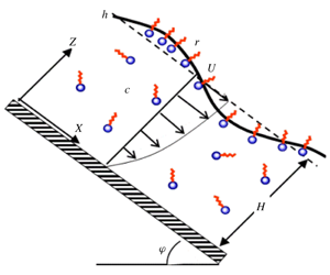
A liquid film laden with soluble surfactant SDS is considered to flow along a flat wall at inclination  $\unicode[STIX]{x1D711}$ with respect to the horizontal (figure 1). The surface tension of the clear liquid is $\unicode[STIX]{x1D6F4}$, whereas that of the solution, designated as $\unicode[STIX]{x1D70E}$, varies along the interface because it is related to the local surface excess concentration, $\unicode[STIX]{x1D6E4}$, of adsorbed surfactant. Alternatively, the surface pressure is defined as $\unicode[STIX]{x1D6F1}=\unicode[STIX]{x1D6F4}-\unicode[STIX]{x1D70E}$. Surface excess concentration is defined according to Gibbs theory (Adamson & Gast Reference Adamson and Gast1997) as the amount of surfactant per unit surface area that is needed to close the mass balance, when considering that the bulk concentration extends right up to the surface. The liquid density, $\unicode[STIX]{x1D70C}$, viscosity, $\unicode[STIX]{x1D707}$, (and kinematic viscosity, $\unicode[STIX]{x1D708}=\unicode[STIX]{x1D707}/\unicode[STIX]{x1D70C}$) are taken as independent of the amount of surfactant, an assumption that is reasonable for concentrations below the critical for the formation of micelles.

Figure 1. Sketch of the flow with the main parameters.
2.1 The flow problem
Two-dimensional dynamics is described by a Cartesian coordinate system ( $X,Z$), with $X$ pointing in the streamwise direction and $Z$ normal to the wall. Film flow along a wall at inclination, $\unicode[STIX]{x1D711}$, with an undisturbed free surface and uniform thickness, $H$, has the classical semiparabolic velocity profile with surface velocity
 $$\begin{eqnarray}U={\displaystyle \frac{g\sin \unicode[STIX]{x1D711}H^{2}}{2\unicode[STIX]{x1D708}}}.\end{eqnarray}$$
Accordingly, the Reynolds number is presently defined as
 $$\begin{eqnarray}Re={\displaystyle \frac{UH}{\unicode[STIX]{x1D708}}}={\displaystyle \frac{g\sin \unicode[STIX]{x1D711}H^{3}}{2\unicode[STIX]{x1D708}^{2}}}.\end{eqnarray}$$
 Lengths are non-dimensionalized with  $H$ (
$H$ ( $x=X/H$, etc.), velocities with $U$, time with $H/U$ and pressure with $\unicode[STIX]{x1D70C}gH\sin \unicode[STIX]{x1D711}$. The dimensionless velocity and pressure fields are $\boldsymbol{u}(x,z,t)=(u,w)$ and $p(x,z,t)$, the location of the interface is $z=h(x,t)$ and that of the wall $z=0$. With this scaling, the continuity and momentum conservation equations become
 $$\begin{eqnarray}\displaystyle & \displaystyle u_{x}+w_{z}=0, & \displaystyle\end{eqnarray}$$
 $$\begin{eqnarray}\displaystyle & \displaystyle Re(u_{t}+uu_{x}+wu_{z})=-2p_{x}+u_{xx}+u_{zz}+2, & \displaystyle\end{eqnarray}$$
 $$\begin{eqnarray}\displaystyle & \displaystyle Re(w_{t}+uw_{x}+ww_{z})=-2p_{z}+w_{xx}+w_{zz}-2\cot \unicode[STIX]{x1D711}, & \displaystyle\end{eqnarray}$$
 where, unless stated otherwise, the subscripts  $x,z,t$ denote partial differentiation.
The boundary conditions are zero velocity at the wall, and the kinematic condition and the balance of forces on the interface,  $z=h(x,t)$. Thus,
 $$\begin{eqnarray}h_{t}+uh_{x}=w\end{eqnarray}$$
and
 $$\begin{eqnarray}\displaystyle & \displaystyle -4u_{x}h_{x}+(u_{z}+w_{x})(1-h_{x}^{2}) & \displaystyle =2\,We\left({\displaystyle \frac{\unicode[STIX]{x1D70E}_{x}}{\unicode[STIX]{x1D6F4}}}\right)\sqrt{1+h_{x}^{2}},\end{eqnarray}$$
 $$\begin{eqnarray}\displaystyle & \displaystyle p+{\displaystyle \frac{u_{x}(1-h_{x}^{2})+(u_{z}+w_{x})h_{x}}{1+h_{x}^{2}}} & \displaystyle =-We\left({\displaystyle \frac{\unicode[STIX]{x1D70E}}{\unicode[STIX]{x1D6F4}}}\right){\displaystyle \frac{h_{xx}}{(1+h_{x}^{2})^{3/2}}},\end{eqnarray}$$
where (2.7) and (2.8) are respectively the components of the force balance tangential and normal to the interface and the Weber number is defined as
 $$\begin{eqnarray}We={\displaystyle \frac{\unicode[STIX]{x1D6F4}}{\unicode[STIX]{x1D70C}g\sin \unicode[STIX]{x1D711}H^{2}}}.\end{eqnarray}$$
2.2 The mass-transfer problem
The surfactant has molar concentration in the bulk  $C(X,Z,T)$ and surface excess concentration $\unicode[STIX]{x1D6E4}(X,T)$; the latter is the concentration at the free-surface location corresponding to $X$ at time $T$. Under equilibrium conditions, the bulk concentration is uniform and related to the surface excess concentration according to the respective adsorption model, $\unicode[STIX]{x1D6E4}_{eq}=\unicode[STIX]{x1D6E4}(C_{eq})$. Details of adsorption modelling are given in the next section.
Departure from equilibrium may cause spatial variation in the surface concentration of surfactant. This spatial variation attributes an elasticity,  $E$, to the interface through the dependence of surface tension on surface concentration. More precisely, Gibbs elasticity is defined as
 $$\begin{eqnarray}E=-\left({\displaystyle \frac{\text{d}\unicode[STIX]{x1D70E}}{\text{d}\ln \unicode[STIX]{x1D6E4}}}\right)_{eq}=-(\unicode[STIX]{x1D6E4}\unicode[STIX]{x1D70E}_{\unicode[STIX]{x1D6E4}})_{eq},\end{eqnarray}$$
where the derivatives are taken in the equilibrium adsorption model. The spatial variation of surface tension that appears in (2.7) may be expressed by the Gibbs elasticity as follows
 $$\begin{eqnarray}\unicode[STIX]{x1D70E}_{x}=\unicode[STIX]{x1D70E}_{\unicode[STIX]{x1D6E4}}\unicode[STIX]{x1D6E4}_{x}=-\left({\displaystyle \frac{E}{\unicode[STIX]{x1D6E4}}}\right)\unicode[STIX]{x1D6E4}_{x}.\end{eqnarray}$$
 Equation (2.11) couples the flow to the mass-transfer problem. At the same time, the departure from equilibrium drives a net flux,  $J(X,T)$, of surfactant between the interface and the bulk.
In order to non-dimensionalize the above variables, surface concentration is scaled with  $\unicode[STIX]{x1D6E4}_{0}=1/\unicode[STIX]{x1D6FA}_{0}$, where $\unicode[STIX]{x1D6FA}_{0}[=]\text{m}^{2}~\text{mol}^{-1}$ is the area covered by an isolated molecule multiplied by the Avogadro number. If the surfactant monolayer is taken as incompressible (hard-sphere model), then $\unicode[STIX]{x1D6E4}_{0}$ is equal to $\unicode[STIX]{x1D6E4}_{\infty }$, the surface concentration at interfacial saturation. However, for a compressible monolayer $\unicode[STIX]{x1D6E4}_{\infty }>\unicode[STIX]{x1D6E4}_{0}$ and $\unicode[STIX]{x1D6E4}_{\infty }$ is an increasing function of surface pressure, $\unicode[STIX]{x1D6F1}$. Using $\unicode[STIX]{x1D6E4}_{0}$, the dimensionless concentrations, Gibbs elasticity and interfacial flux are defined respectively as $\unicode[STIX]{x1D6FE}(x,t)=\unicode[STIX]{x1D6E4}(X,T)/\unicode[STIX]{x1D6E4}_{0}$, $c(x,z,t)=C(X,Z,T)H/\unicode[STIX]{x1D6E4}_{0}$, $e=E/\unicode[STIX]{x1D6F4}=-\unicode[STIX]{x1D6FE}(\unicode[STIX]{x1D70E}/\unicode[STIX]{x1D6F4})_{\unicode[STIX]{x1D6FE}}$ and $j(x,t)=J(X,T)\unicode[STIX]{x1D6E4}_{0}U/H$.
Mass conservation of adsorbed and dissolved surfactant is imposed by the following two advection–diffusion equations (Pereira & Kalliadasis Reference Pereira and Kalliadasis2008b), equation (2.12) for the bulk and (2.13) for the interface:
 $$\begin{eqnarray}\displaystyle & \displaystyle c_{t}+uc_{x}+wc_{z}=Pe_{b}^{-1}(c_{xx}+c_{zz}), & \displaystyle\end{eqnarray}$$
 $$\begin{eqnarray}\displaystyle & \displaystyle \unicode[STIX]{x1D6FE}_{t}+u\unicode[STIX]{x1D6FE}_{x}+\unicode[STIX]{x1D6FE}(\unicode[STIX]{x1D6FB}_{s}\boldsymbol{\cdot }\boldsymbol{u})=Pe_{s}^{-1}\unicode[STIX]{x1D6FB}_{s}^{2}\unicode[STIX]{x1D6FE}+j. & \displaystyle\end{eqnarray}$$
 Here,  $Pe_{b}=Re\,Sc_{b}=UH/D_{b}$ and $Pe_{s}=Re\,Sc_{s}=UH/D_{s}$ are the Péclet numbers of the bulk and the interface, $D_{b},D_{s}$ are the bulk and surface diffusivities and $j$ is the dimensionless interfacial flux. The surface gradient, $\unicode[STIX]{x1D6FB}_{s}$, is defined as $\unicode[STIX]{x1D6FB}_{s}=(\boldsymbol{I}-\boldsymbol{n}\boldsymbol{n})\boldsymbol{\cdot }\unicode[STIX]{x1D735}$ in terms of the local unit normal to the interface, $\boldsymbol{n}$.
The no-penetration condition is applied at the wall, where  $z=0$
$z=0$
 $$\begin{eqnarray}c_{z}=0\end{eqnarray}$$
 and two concentration boundary conditions are imposed at the interface,  $z=h(x,t)$. One expresses the net flux of surfactant in terms of the bulk concentration gradient
 $$\begin{eqnarray}j=-Pe_{b}^{-1}(\unicode[STIX]{x1D735}\boldsymbol{\cdot }\boldsymbol{n})_{z=h},\end{eqnarray}$$
and the other assumes equilibrium between subsurface and adsorbed concentrations,
 $$\begin{eqnarray}c(z=h)=c_{eq}(\unicode[STIX]{x1D6FE}).\end{eqnarray}$$
 The assumption of interfacial equilibrium could be relaxed by taking the net flux which results from an imbalance between kinetic rates of adsorption and desorption (Borwankar & Wasan Reference Borwankar and Wasan1988). However, this phenomenological generalization that takes into account kinetic resistance to adsorption, would not make any difference below frequencies  $f\sim 100~\text{Hz}$ (Wantke & Fruhner Reference Wantke and Fruhner2001). This value is two orders of magnitude above the maximum wave frequency of the experiments to be considered.
2.3 Linear stability analysis
A base state for the present problem corresponds to Nusselt flow with flat interface and uniform bulk concentration of surfactant in equilibrium with the adsorbed monolayer. For small departures from this base state, the equations and boundary conditions may be linearized and the travelling disturbances expressed as normal modes in terms of the wavelength,  $L$, or the wavenumber, $k=2\unicode[STIX]{x03C0}/L$, and the complex phase velocity, $V$, of the interface deformation.
The relevant Orr–Sommerfeld eigenvalue problem has been formulated and solved numerically by a Galerkin finite-element method (Karapetsas & Bontozoglou Reference Karapetsas and Bontozoglou2013), the main outcome being the critical Reynolds number for the primary instability,  $Re_{cr}$, as a function of the disturbance wavenumber. The same procedure is used for the predictions reported in the present work. It is recalled that the above temporal stability analysis provides the correct critical Reynolds number for the general initial-value problem (Charru Reference Charru2011), so it is also appropriate for the presently considered experiment, where periodic disturbances are introduced at a fixed upstream location and are convected by the flow.
Film flow is known to be susceptible to a longwave instability, so analysis of the stability problem in the limit  $k\rightarrow 0$ may be very relevant. This analysis has been performed (Wei Reference Wei2005; Karapetsas & Bontozoglou Reference Karapetsas and Bontozoglou2014; Bontozoglou Reference Bontozoglou2018) and provides insights on the mechanism of the instability. More specifically, it has been shown that disturbance of the adsorbed monolayer is initiated by the velocity perturbation imposed on the base flow by the travelling interfacial disturbance. The interface deformation does not by itself trigger any change in concentration because surface dilatation is second-order in the deformation amplitude, i.e. it is linearly negligible.
The main result of the longwave analysis is the following prediction of  $Re_{cr}$:
 $$\begin{eqnarray}Re_{c}={\displaystyle \frac{5}{4}}\cot \unicode[STIX]{x1D711}+{\displaystyle \frac{15}{4}}We\,e\left({\displaystyle \frac{3}{3+4\unicode[STIX]{x1D6EC}}}\right),\end{eqnarray}$$
 which corresponds to waves with zero growth rate,  $kV_{i}=0$, and dimensionless travelling speed, $V_{r}=2$. Term $e=E/\unicode[STIX]{x1D6F4}$ is the dimensionless Gibbs elasticity, as defined by equation (2.10), and $\unicode[STIX]{x1D6EC}$ is a solubility parameter, defined according to the relation
 $$\begin{eqnarray}\unicode[STIX]{x1D6EC}=\left({\displaystyle \frac{\text{d}c}{\text{d}\unicode[STIX]{x1D6FE}}}\right)_{eq}=H\left({\displaystyle \frac{\text{d}C}{\text{d}\unicode[STIX]{x1D6E4}}}\right)_{eq}.\end{eqnarray}$$
 It is zero for an insoluble surfactant and increases with solubility. As with Gibbs elasticity,  $\unicode[STIX]{x1D6EC}$ is calculated at the equilibrium conditions of the base flow.
An important consequence of the longwave assumption is that mass exchange between the interface and the bulk is at leading order negligible, i.e. local equilibrium with the interface is established at every streamwise location because of the slow variation along the wavelength. In this limit, the bulk concentration varies only in the flow direction, and the amplitudes of concentration perturbations in the bulk and at the monolayer are in a ratio equal to  $\unicode[STIX]{x1D6EC}$.
3 Modelling of adsorption
The Frumkin isotherm is used to describe adsorption equilibrium. Thus, interface and bulk concentrations are related by
 $$\begin{eqnarray}C={\displaystyle \frac{1}{K\text{e}^{2a\unicode[STIX]{x1D703}}}}\left({\displaystyle \frac{\unicode[STIX]{x1D6E4}}{\unicode[STIX]{x1D6E4}_{\infty }-\unicode[STIX]{x1D6E4}}}\right)={\displaystyle \frac{1}{K\text{e}^{2a\unicode[STIX]{x1D703}}}}\left({\displaystyle \frac{\unicode[STIX]{x1D703}}{1-\unicode[STIX]{x1D703}}}\right),\end{eqnarray}$$
and the corresponding equation of state is
 $$\begin{eqnarray}{\displaystyle \frac{\unicode[STIX]{x1D6F4}-\unicode[STIX]{x1D70E}}{RT\unicode[STIX]{x1D6E4}_{\infty }}}={\displaystyle \frac{\unicode[STIX]{x1D6F1}}{RT\unicode[STIX]{x1D6E4}_{\infty }}}=-\ln (1-\unicode[STIX]{x1D703})-a\unicode[STIX]{x1D703}^{2}.\end{eqnarray}$$
 (All the equations of this section refer to equilibrium conditions, i.e.  $C_{eq},\unicode[STIX]{x1D6E4}_{eq}$, but the subscript ‘eq’ is omitted for simplicity.) Here, $K$ is the adsorption constant, $a$ is the interaction constant for adsorbed molecules and $\unicode[STIX]{x1D6E4}_{\infty }$ is the surface concentration at interfacial saturation. Term $\unicode[STIX]{x1D703}=\unicode[STIX]{x1D6E4}/\unicode[STIX]{x1D6E4}_{\infty }$ is the monolayer coverage, which may be expressed as $\unicode[STIX]{x1D703}=\unicode[STIX]{x1D6E4}\unicode[STIX]{x1D6FA}$ in terms of $\unicode[STIX]{x1D6FA}=1/\unicode[STIX]{x1D6E4}_{\infty }$, the molar area of adsorbed surfactant in the state of saturation.
If the adsorbed monolayer is taken as incompressible, then  $\unicode[STIX]{x1D6E4}_{\infty }\equiv \unicode[STIX]{x1D6E4}_{0},\unicode[STIX]{x1D703}\equiv \unicode[STIX]{x1D6FE}$, and both $e$ and $\unicode[STIX]{x1D6EC}$ tend to infinity in the limit of high surface coverage. Thus, application of (2.17) to predict $Re_{cr}$ becomes questionable. What is worse, the predicted high values of $e$ and $\unicode[STIX]{x1D6EC}$ when $\unicode[STIX]{x1D703}\rightarrow 1$ are in order-of-magnitude disagreement with data (Wantke et al. Reference Wantke, Fruhner, Fang and Lunkenheimer1998). As zero compressibility is equivalent to infinite elasticity, Kovalchuk et al. (Reference Kovalchuk, Loglio, Fainerman and Miller2004) have proposed that the adsorbed monolayer be characterized by a linear compressibility, $\unicode[STIX]{x1D700}$, according to the relation
 $$\begin{eqnarray}\unicode[STIX]{x1D6FA}=\unicode[STIX]{x1D6FA}_{0}(1-\unicode[STIX]{x1D700}\unicode[STIX]{x1D6F1}).\end{eqnarray}$$
 As discussed in Fainerman, Miller & Kovalchuk (Reference Fainerman, Miller and Kovalchuk2002), the dependence of molecular area on surface pressure has been demonstrated by synchrotron X-ray diffraction (grazing incidence X-ray diffraction) for the case of insoluble amphiphilic molecules in the condensed state. Extending the notion to saturated monolayers in the liquid state, it can be hypothesized that surface compressibility,  $\unicode[STIX]{x1D700}$, is related to the tilt angle of the adsorbed molecules with respect to the normal. During compression of the monolayer, the tilt angle decreases; therefore, the area per molecule becomes smaller. The value of surface compressibility, $\unicode[STIX]{x1D700}$, depends on the specific surfactant molecule and varies in the range $\unicode[STIX]{x1D700}=4{-}10~\text{m}~\text{N}^{-1}$ (Fainerman et al. Reference Fainerman, Miller and Kovalchuk2002).
Using (3.2) and the concept of Gibbs dividing surface on the interface, it may be shown (Kovalchuk et al. Reference Kovalchuk, Loglio, Fainerman and Miller2004) that the isotherm, equation (2.18), remains invariant, but the equation of state (former (3.1)) becomes
 $$\begin{eqnarray}{\displaystyle \frac{\unicode[STIX]{x1D6F1}\unicode[STIX]{x1D6FA}_{0}}{RT}}\left(1-{\displaystyle \frac{\unicode[STIX]{x1D700}\unicode[STIX]{x1D6F1}}{2}}\right)=-\ln (1-\unicode[STIX]{x1D703})-a\unicode[STIX]{x1D703}^{2}.\end{eqnarray}$$
 However, note that  $\unicode[STIX]{x1D6E4}$ in (2.18) is now given by
 $$\begin{eqnarray}\unicode[STIX]{x1D6E4}={\displaystyle \frac{\unicode[STIX]{x1D703}}{\unicode[STIX]{x1D6FA}_{0}(1-\unicode[STIX]{x1D700}\unicode[STIX]{x1D6F1})}}.\end{eqnarray}$$
Combining (2.18), (3.3) and (3.4), Gibbs elasticity is found equal to
 $$\begin{eqnarray}e=\left[{\displaystyle \frac{\unicode[STIX]{x1D6F4}\unicode[STIX]{x1D6FA}_{0}}{RT}}{\displaystyle \frac{(1-\unicode[STIX]{x1D700}\unicode[STIX]{x1D6F1})}{\left({\displaystyle \frac{\unicode[STIX]{x1D703}}{1-\unicode[STIX]{x1D703}}}-2a\unicode[STIX]{x1D703}^{2}\right)}}+{\displaystyle \frac{\unicode[STIX]{x1D6F4}\unicode[STIX]{x1D700}}{1-\unicode[STIX]{x1D700}\unicode[STIX]{x1D6F1}}}\right]^{-1}.\end{eqnarray}$$
According to Gibbs theory for an ideal solution, elasticity and solubility are related by
 $$\begin{eqnarray}{\displaystyle \frac{\text{d}\unicode[STIX]{x1D6E4}}{\text{d}C}}={\displaystyle \frac{RT\unicode[STIX]{x1D6E4}^{2}}{CE}}\quad \text{or}\quad \unicode[STIX]{x1D6EC}={\displaystyle \frac{\unicode[STIX]{x1D6F4}\unicode[STIX]{x1D6FA}_{0}}{RT}}{\displaystyle \frac{ce}{\unicode[STIX]{x1D6FE}^{2}}}.\end{eqnarray}$$
 The expression for Gibbs elasticity, equation (3.5), represents two elasticity mechanisms in series, the first on the right-hand side is compositional, i.e. related to spatial variations in surface concentration, and the second on the right-hand side is intrinsic, i.e. related to the surface compressibility of the monolayer. Upon saturation, i.e. when  $\unicode[STIX]{x1D703}\rightarrow 1$, the interface retains finite elasticity due to the intrinsic contribution.
4 Key characteristics of the experimental set-up
Experiments by Georgantaki et al. (Reference Georgantaki, Vlachogiannis and Bontozoglou2016) were done in a 3000 mm long by 450 mm wide inclined channel. The liquid film formed at the entrance by overflow from a manifold open to the atmosphere. Liquid exiting at the bottom of the channel was collected in a large tank and was recirculated to the inlet manifold with the help of a submersible pump.
The above set-up avoids two potential problems related to SDS properties. The first has to do with deviations from equilibrium surfactant concentration at the inlet. If, for example, the film were formed by extrusion through a thin slot, the newly created interface would be temporarily clean and would thus trigger Marangoni stresses pulling the surface towards the upstream direction. In the presently considered experiment, the inlet manifold with its free surface provides enough residence time for equilibrium to be established.
The second potential problem has to do with the slow hydrolysis of SDS to dodecanol, a surfactant that is stronger than SDS and is practically insoluble. This reaction results in a distinct ageing effect, which starts to affect surface tension roughly 100–500 s after formation of a new interface and grows in significance with time (Fainerman et al. Reference Fainerman, Lylyk, Aksenenko, Petkov, Yorke and Miller2010).
Complications resulting from this process are avoided in the experiment of Georgantaki et al. (Reference Georgantaki, Vlachogiannis and Bontozoglou2016) because of the use of a large collection tank and of a submersible pump for recirculating the liquid. The tank provides enough residence time for the dodecanol to separate from the bulk and gather at the surface, while the submersible pump has its suction port near the bottom of the tank and thus delivers pure solution of SDS to the channel inlet. The sum of the residence time in the entrance manifold and the fly time along the channel is at maximum 120 s, which is too short for dodecanol to have any noticeable effect.
Measurements of the surface tension of samples taken from the flowing liquid film were used by Georgantaki et al. (Reference Georgantaki, Vlachogiannis and Bontozoglou2016) to characterize the experimental conditions. According to the above argument, these measurements were not affected by the formation of dodecanol. It is noted that surface tension – and not bulk surfactant concentration – is the most reliably determined independent variable in those experiments. Though the quantity of SDS added each time to the flow loop is known, additional amounts remain in pockets of liquid trapped in the piping and connections during emptying and refilling of the facility. Thus, all the data from the experimental paper are reported below in terms of the measured surface tension.
5 Comparisons at the longwave limit
The Frumkin isotherm, when applied to an ionic surfactant such as SDS, is a pseudo non-ionic model. Thus, the values of parameters  $K$ and $a$ vary strongly with the solution salinity, $C_{s}$. For the present purposes, use is made of the systematic best-fit results for SDS by Prosser & Franses (Reference Prosser and Franses2001) for salinities $C_{s}=0,10,100$ and 500 mM. This variation in the model parameters may be physically understood by considering that high salinity weakens electrostatic repulsions and facilitates surface adsorption. Thus, the same reduction in surface tension is achieved at lower monomer concentrations in the bulk.
The measurements by Georgantaki et al. (Reference Georgantaki, Vlachogiannis and Bontozoglou2016) were taken using brackish water, which was characterized by its electric conductivity. For most of the experimental campaign, the conductivity was around  $3000~\unicode[STIX]{x03BC}\text{S}~\text{cm}^{-1}$ (corresponding to a salinity $C_{s}=26~\text{mM}$), while for some runs the conductivity was somewhat lower (minimum value measured $2400~\unicode[STIX]{x03BC}\text{S}~\text{cm}^{-1}$, $C_{s}=21~\text{mM}$). Based on these experimental conditions, interpolated values of the adsorption constant are used in the stability computations, spanning the interval from $K=11.0~\text{m}^{3}~\text{mol}^{-1}$ for $C_{s}=26~\text{mM}$ to $K=8.0~\text{m}^{3}~\text{mol}^{-1}$ for $C_{s}=21~\text{mM}$, while the interaction constant is taken as $a=0.4$. The molar area of adsorbed molecules varies little with salinity, so it is expressed by the constant value $\unicode[STIX]{x1D6E4}_{0}=4.15~\text{mol}~\text{m}^{-2}$, which is consistent with the size of the SDS molecule (Prosser & Franses Reference Prosser and Franses2001).
Georgantaki et al. (Reference Georgantaki, Vlachogiannis and Bontozoglou2016) have reported measurements of wave properties for channel inclination  $\unicode[STIX]{x1D711}=5^{\text{o}}$ and surface tension ranging from 38 to $68~\text{mN}~\text{m}^{-1}$. Small-amplitude propagating surface waves were created by introduction of inlet disturbances with frequencies in the range $f=0.1{-}1.0~\text{Hz}$. The streamwise evolution of the wave amplitude was recorded by conductance probes and the critical Reynolds number, $Re_{cr}$, corresponding to zero amplification, was determined. The phase speed and wavelength of propagating waves were determined from the time-lag, $\unicode[STIX]{x0394}t_{l}$, of the signals of two probes, separated by a small distance, $\unicode[STIX]{x0394}x$, in the streamwise direction. Then, $V=\unicode[STIX]{x0394}x/\unicode[STIX]{x0394}t_{l}$ and $L=V/f$.
The relevance of these data to the longwave limit is examined first by considering the phase speed and wavelength of travelling disturbances. To this end, the experimental dimensionless wavenumber,  $\hat{k}_{exp}=2\unicode[STIX]{x03C0}H/L$, is plotted in figure 2 as a function of $Re$ (points), and is compared to the theoretical prediction, $\hat{k}_{long}=2\unicode[STIX]{x03C0}H/L=2\unicode[STIX]{x03C0}Hf/V_{r}\approx \unicode[STIX]{x03C0}Hf/U$ (lines). Based on the results plotted in figure 2, the data are classified in three categories. For $f=1~\text{Hz}$, there is clear disagreement, pointing to a finite-wavelength effect. On the contrary, data and theory are in satisfactory agreement for $f=0.75$ and 0.50 Hz, indicating that the longwave limit has been reached.
For smaller inlet frequencies,  $f=0.125{-}0.25~\text{Hz}$, there is again disagreement, but this is known to occur because of three-dimensional (sidewall) effects. More specifically, it has been shown (Leontidis et al. Reference Leontidis, Vatteville, Vlachogiannis, Andritsos and Bontozoglou2010; Georgantaki et al. Reference Georgantaki, Vatteville, Vlachogiannis and Bontozoglou2011) that when the wavelength exceeds twice the channel width ( $L>2W$), sidewalls start to affect the characteristics of travelling disturbances, reducing their phase speed and rendering them more stable. Thus, in the following, we neglect the very long waves, which correspond to $f=0.125{-}0.25~\text{Hz}$ and deviate from two-dimensionality.
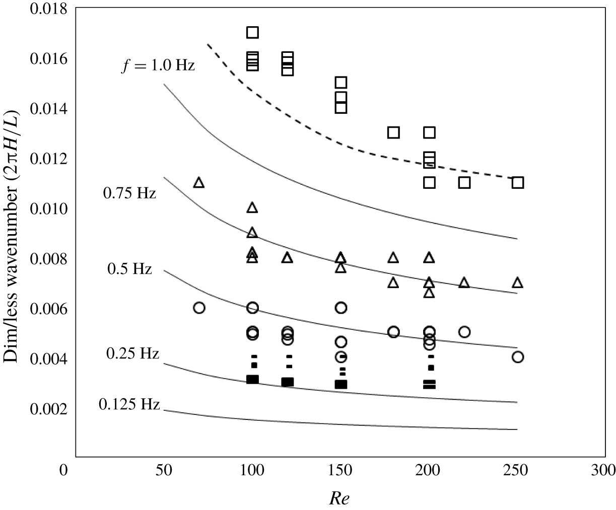
Figure 2. Dimensionless wavenumbers as determined from the data for frequencies  $f=1~\text{Hz}$ (▫), $0.75~\text{Hz}$ (▵), $0.5~\text{Hz}$ (○), $0.25~\text{Hz}$ (-) and $0.125~\text{Hz}$ (–) compared to predictions of longwave theory. The dashed curve is the prediction for $f=1~\text{Hz}$, taking into account finite-wavelength effects.
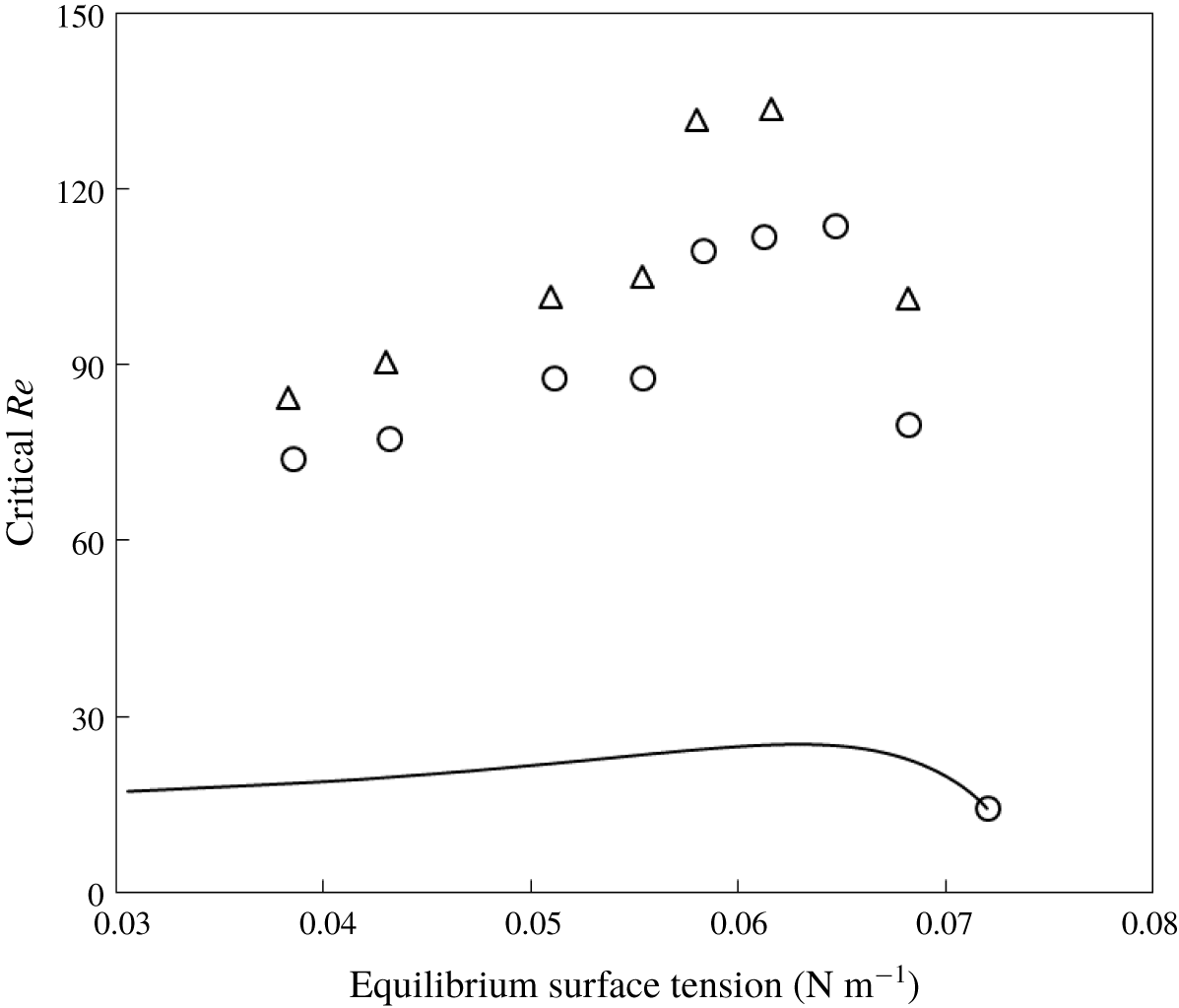
Figure 3. Measurements of the critical Reynolds number for inlet frequencies  $f=0.75$ Hz (▵) and 0.5 Hz (○), compared to the prediction of longwave theory. The lowest open circle corresponds to experiments without surfactant.
Following the agreement in wave characteristics for  $f=0.50{-}0.75~\text{Hz}$, the measured critical Reynolds number, $Re_{cr,exp}$, for the primary instability is compared to the longwave prediction, equation (2.17), in figure 3. Here, the $x$-axis is the equilibrium surface tension for the undisturbed aqueous SDS solution and the $y$-axis is the critical Reynolds number. It is readily observed that the data for the two frequencies differ from each other, an indication that there is still a wavelength effect. What is worse, the longwave prediction fails by almost an order of magnitude.
The above contradictory results are reconciled if it is realized that the flow and mass-transfer problems have transport properties that differ by orders of magnitude. Kinematic viscosity (taken equal to that of pure water) is  $\unicode[STIX]{x1D708}\approx 0.9\times 10^{-6}~\text{m}^{2}~\text{s}^{-1}$ and diffusivity of SDS molecules is estimated as $D_{b}\approx 5\times 10^{-10}~\text{m}^{2}~\text{s}^{-1}$ (Weinheimer, Evans & Cussler Reference Weinheimer, Evans and Cussler1981; Barhoum & Yethiraj Reference Barhoum and Yethiraj2010), resulting in a Schmidt number $Sc_{b}\approx 1800$.
With these values of molecular transport, flow perturbations with typical period  $\unicode[STIX]{x1D70F}=1{-}10~\text{s}$ – as in the experiments presently considered – have penetration depth, $z_{flow}\sim \sqrt{\unicode[STIX]{x1D708}\unicode[STIX]{x1D70F}}\approx 1000{-}3000~\unicode[STIX]{x03BC}\text{m}$, i.e. larger than the liquid film thickness, $H\sim 500{-}1000~\unicode[STIX]{x03BC}\text{m}$. On the contrary, perturbations in surface concentration have penetration depth $z_{mass}\sim \sqrt{D_{b}\unicode[STIX]{x1D70F}}\approx 20{-}75~\unicode[STIX]{x03BC}\text{m}$, which is an order of magnitude smaller than the film thickness. Thus, a major assumption of the longwave analysis, i.e. that local equilibrium is established at every streamwise location between the interface and the bulk concentrations, is not valid for the data of Georgantaki et al. (Reference Georgantaki, Vlachogiannis and Bontozoglou2016). It is interesting to note that longwave theory fails despite the fact that the formal criterion, the ratio of film thickness to wavelength, is as low as $H/L\sim 10^{-3}$.
An equivalent explanation can be provided by scaling the dimensional governing equations according to longwave theory, i.e. using  $L$ for the $x$- and $H$ for the $z$-direction. Then the convective terms in the $x$-momentum, equation (2.4), and the scalar transport, equation (2.12), are multiplied respectively by $Re(H/L)$ and $Pe_{b}(H/L)$. Given that $Pe_{b}=ReSc_{b}\gg Re$, scalar transport is expected to converge to the zero wavenumber limit $(H/L\rightarrow 0)$ at a much smaller rate than momentum transport.
6 Incorporation of finite-wavelength effects
Next, predictions of linear stability theory are produced that take into account the wavelength of the disturbance. The question to be investigated is whether finite-wavelength effects suffice to explain the behaviour observed in the experiment. The procedure followed is the numerical solution of the relevant Orr–Sommerfeld eigenvalue problem by a Galerkin finite-element method, as described in detail by Karapetsas & Bontozoglou (Reference Karapetsas and Bontozoglou2013).
Given that temporal stability is formulated in terms of the wavenumber, whereas data are taken for specific frequencies,  $f$, an iteration is necessary during application of the numerical solver. An initial guess for the wavenumber is made using the longwave result, $\hat{k}_{long}=2\unicode[STIX]{x03C0}Hf/V_{r}\approx \unicode[STIX]{x03C0}Hf/U$, and the wave speed, $V$, for the specific $\mathit{Re}$ considered is computed. Whereas the imaginary part of $V$ gives the growth rate of the disturbance, the real part, in combination with the frequency, $f$, provides an updated value for the wavenumber. The improved prediction of wave properties for the highest inlet frequency, $f=1.0~\text{Hz}$, for which finite-wavelength effects were shown to be important, is demonstrated in figure 2 as a dashed line.
The comparison between predictions of the stability threshold, using the above procedure, and measurements is shown in figure 4. Data (points) are included for all three frequencies that obey two-dimensional dynamics, i.e.  $f=0.5,0.75$ and $1.0~\text{Hz}.$ Molecular transport in the bulk is expressed by $Sc_{b}=1800$, and surface transport by $\mathit{Sc}_{\text{s}}=10\,000$, which turns out to have a negligible effect. Compressibility of the adsorbed monolayer is taken as $\unicode[STIX]{x1D700}=6~\text{m}~\text{N}^{-1}$, whereas its neglect ( $\unicode[STIX]{x1D700}=0~\text{m}~\text{N}^{-1}$) gives the results shown by dotted lines.

Figure 4. Measurements of the critical Reynolds number for inlet frequencies  $f=1$ Hz (▪), 0.75 Hz ( ▲ ) and 0.5 Hz (●), compared to predictions of linear theory, with monolayer compressibility $\unicode[STIX]{x1D700}=6~\text{m}~\text{N}^{-1}$ (continuous lines) and $\unicode[STIX]{x1D700}=0$ (dotted lines).
The data points for  $\unicode[STIX]{x1D70E}=51.0,55.4$ and $58.0~\text{mN}~\text{m}^{-1}$ were taken with water of lower conductivity than $3000~\unicode[STIX]{x03BC}\text{S}~\text{cm}^{-1}$ ( $2600,2400$ and $2850~\unicode[STIX]{x03BC}\text{S}~\text{cm}^{-1}$, respectively), and should be compared to an accordingly modified prediction. In order not to overcrowd figure 4 with additional stability curves corresponding to the lower salinities, these data are ‘regularized’ by the expression
 $$\begin{eqnarray}Re_{exp,reg}=Re_{exp,orig}(Re_{pred,3000}/Re_{pred,conductiviy}).\end{eqnarray}$$
 As is demonstrated by figure 4, predictions improve dramatically with the inclusion of finite-wavelength effects. In particular,  $Re_{cr}$ at maximum stabilization is now close to the data, and the agreement holds for all three frequencies tested. Thus, it is concluded that the slow molecular diffusion of surfactant is responsible for the deviation from local equilibrium in the normal direction and the ensuing enhanced stability of the film compared to the longwave limit.
The significance of monolayer compressibility is very notable. Its inclusion in the prediction leads to distinctively slower decline of  $Re_{cr}$ with increasing surface coverage (decreasing surface tension). The actual value used, $\unicode[STIX]{x1D700}=6~\text{m}~\text{N}^{-1}$, is a realistic estimate confirmed by independent measurements (Fainerman et al. Reference Fainerman, Miller and Kovalchuk2002) and is observed to result in quantitative agreement with the data.
The effect of salinity on the prediction of  $Re_{cr}$ for the primary instability enters the problem through the parameters $K$ and $a$ of the adsorption isotherm (2.18) and is examined more systematically in figure 5. The results shown correspond to $C_{s}=10,26$ and 100 mM and indicate significant stabilization. This trend is explained when it is considered that SDS is actually an ionic surfactant and the adsorbed ions create an electric double-layer. With increasing salinity, the thickness of the double-layer decreases and the addition of ions to the surface becomes easier. As a result, lower bulk concentrations are needed to create a specific surface concentration. Lower bulk concentrations lead to slower mass exchange with the interface, and thus to stronger stabilizing Marangoni stresses.
7 Concluding remarks
Linear stability theory of gravity-driven film flow laden with a soluble surfactant is set in perspective with literature measurements taken with aqueous solutions of SDS. This flow is characterized by a non-monotonic variation of the critical Reynolds number with surfactant loading. A drastic increase in  $Re_{cr}$ occurs with the addition of small amounts of SDS, but then a maximum is reached and subsequently $Re_{cr}$ declines slowly. This behaviour is understood as the outcome of two competing effects: with the addition of surfactant, the surface coverage (and thus the potential for Marangoni stresses) increases. However, the concomitant increase in bulk concentration intensifies mass exchange with the interface, which mitigates surface-tension gradients.

Figure 5. Prediction of the effect of solution salinity on the critical Reynolds number of the primary instability for disturbances with frequency  $f=0.5~\text{Hz}$. The case $C_{s}=26~\text{mM}$ corresponds to the experiments of Georgantaki et al. (Reference Georgantaki, Vlachogiannis and Bontozoglou2016).
Quantitative comparison with the zero wavenumber version of linear stability is satisfactory for wave properties but fails in the prediction of  $Re_{cr}$ by roughly an order of magnitude. This discrepancy is understood in terms of the large difference between momentum and mass diffusivities (high Schmidt number) and indicates that the assumption of infinite wavelength is far more restrictive for the mass transfer than for the flow problem. As the values of molecular diffusivity of most surfactants are in the same order (Kovalchuk et al. Reference Kovalchuk, Loglio, Fainerman and Miller2004), this conclusion holds in general. Thus, longwave analysis of the behaviour of soluble surfactants needs always to be approached with caution.
Consideration of finite-wavelength effects and inclusion of finite compressibility of the adsorbed monolayer brings predictions to quantitative agreement with the experimental data for all disturbance frequencies tested. It also demonstrates a strong stabilizing effect of salinity of the aqueous solution. High salinity facilitates surface adsorption by weakening electrostatic repulsions, and thus achieves the same reduction in surface tension at lower monomer concentrations in the bulk.
As was presently shown, the role of a soluble surfactant on the linear stability of liquid film flow has mainly to do with the creation of Marangoni stresses, while the direct effect of lowering (the mean) surface tension appears negligible. Though this may come as no surprise for a longwave instability, it is noted that three-dimensional effects, imposed by the sidewalls, may make the actual value of surface tension relevant. For example, Georgantaki et al. (Reference Georgantaki, Vatteville, Vlachogiannis and Bontozoglou2011) showed that for narrow enough channels the primary instability of film flow becomes also a function of Kapitza number.
Finally, even if the lowering of surface tension does not have a direct effect on the primary instability, it may eventually affect the evolution of an unstable film. A relevant case is the formation of precursor ripples in front of solitary humps of low-viscosity fluids, where capillary forces balance the gravity-induced inertia of the fluid. Indeed, it was observed by Georgantaki et al. (Reference Georgantaki, Vlachogiannis and Bontozoglou2012) that the addition of the highly soluble surfactant isopropanol resulted in strong amplification of the precursor ripples.
Acknowledgements
The stimulating comments and suggestions of the referees are gratefully acknowledged.
Declaration of interests
The authors report no conflict of interest.


 Open access