2.1. Governing equations

Our simulation geometry in non-dimensional units is shown in figure 1(a,b). It replicates the experimental geometry (see e.g. figure 1 of Lefauve et al. (Reference Lefauve, Partridge and Linden2019) in dimensional units), which consists of a duct of square cross-section with internal height $H$, width $W$ and length $L$ connecting two large reservoirs with fluids at densities $\rho _0\pm \Delta \rho /2$ (white and blue shaded areas in figure 1a). To match previous experimental studies of SID, we non-dimensionalise all lengths by the duct half-height $H/2$, making the duct non-dimensional length, height and width $2A\times 2B\times 2$, respectively, where $A\equiv L/H$ and $B=W/H$ are the streamwise and spanwise aspect ratios, respectively. We also non-dimensionalise (i) the velocities by the fixed buoyancy velocity scale $\Delta U/2 \equiv \sqrt {g^\prime H}$ (where $g^\prime =g\Delta \rho /\rho _0$ is the reduced gravity and $\rho _0$ is the reference density); (ii) the time by the advective time unit (ATU) $H/\Delta U$; (iii) the density variations around the reference $\rho _0$ by $\Delta \rho /2$; and (iv) the pressure by $\rho _0(\Delta U/2)^2$. Note that the $x$ axis (the streamwise direction) is aligned along the duct, whereas gravity points downwards at an angle $\theta$ from the $-z$ axis (the vertical direction in the frame of the duct); hence in these duct coordinates $\boldsymbol {g}=g {\hat {\boldsymbol {g}}}=g(\sin \theta, 0, -\cos \theta )$.

Figure 1. Schematics of SID geometry in non-dimensional units. (a) Overview of the rectangular simulation domain of dimensions $L_x,L_y,L_z$ within which immersed boundaries create a square duct of dimensions $2A\times 2\times 2$. (b) Detail of the duct geometry and coordinate system. (c) Shape of the different reservoirs considered in this paper (benchmark, AR, BR and SR), with a total domain length $L_x=2(A+L^r_x)$. All numerical parameters are summarised in table 1.

Table 1. Summary of the DNS. From left to right: reservoir geometry (case) as shown in figure 1(c); Reynolds number; tilt angle; duct streamwise aspect ratio; duct spanwise aspect ratio; reservoir size; grid size of the entire computational domain; and forcing parameters: streamwise length of forcing ($l_f$) and time scales controlling momentum ($\eta _u$) and density forcing ($\eta _\rho$) in (2.5)–(2.6). Bold font and superscripts denote the most used DNS.

The resulting non-dimensional governing equations for our DNS are the Navier–Stokes equations under the Boussinesq approximation:

(2.1)$$\begin{gather} \boldsymbol{\nabla} \boldsymbol{\cdot} \boldsymbol{u} = 0, \end{gather}$$

(2.2)$$\begin{gather}\frac{{\rm D} \boldsymbol{u}}{{\rm D} t} ={-} \boldsymbol{\nabla}p + \frac{1}{Re} \nabla^{2}\boldsymbol{u}+ {Ri} \, \rho \, {\hat{\boldsymbol{g}}} - \boldsymbol{F}_u, \end{gather}$$

(2.3)$$\begin{gather}\frac{{\rm D} \rho}{{\rm D} t} = \frac{1}{{Re \,Pr}} \nabla^{2}\rho - F_\rho, \end{gather}$$

where the material derivative is ${\rm D}/{\rm D}t \equiv \partial _t+\boldsymbol {u}\boldsymbol {\cdot } \boldsymbol {\nabla }$, the velocity is $\boldsymbol {u}=(u,v,w)$ in the non-dimensional coordinate system $\boldsymbol {x}=(x,y,z)$ aligned with the duct, the non-dimensional pressure is $p$ and the non-dimensional density variation around the mean is $\rho$ (bounded between $-1$ and $1$). The forcing terms $\boldsymbol {F}_u$ and $F_\rho$ used to maintain the quasi-steady exchange flows are described in § 2.2.

The non-dimensional Reynolds, Richardson and Prandtl numbers are related to the dimensional experimental parameters as follows:

(2.4a–c)\begin{equation} {Re}\equiv \frac{\dfrac{\Delta U}{2}\dfrac{H}{2}}{\nu} \equiv \dfrac{\sqrt{g'H}H}{2\nu}, \quad {Ri}\equiv \frac{\dfrac{g}{\rho_0}\dfrac{\Delta\rho}{2}\dfrac{H}{2}}{\left(\dfrac{\Delta U}{2}\right)^2}\equiv \frac{1}{4}, \quad {Pr}\equiv \frac{\nu}{\kappa} \equiv 7, \end{equation}

where $\nu$ is the kinematic viscosity and $\kappa$ is the mass diffusivity. Previous studies of SID showed that the streamwise velocity scales with $\Delta U/2$, motivating this definition of Reynolds number. The Richardson number is always equal to 1/4 due to the definition of $\Delta U$. The Prandtl number in all simulations was set to ${Pr}=7$, approximately representative of temperature stratification in water at room temperature. For a given duct and reservoir geometry, there are two remaining free non-dimensional parameters: the tilt angle $\theta$ and the Reynolds number ${Re}$ (based on the driving density difference $\Delta \rho$).

2.2. Artificial restoring of the exchange flow

The exchange flow in the duct is driven by the hydrostatic longitudinal pressure gradient and by the longitudinal gravitational acceleration $g\sin \theta$. In the context of a two-layer flow, the along-duct component of gravity accelerates the heavier layer rightwards (downhill) and the lighter layer leftwards (uphill). The role of the hydrostatic pressure gradient turns out to be more intricate and is examined in § 5.3. In the experiments, the flow inside the duct is sustained over long time periods (typically several hundred ATUs) until the discharged fluids accumulated in the large reservoirs have reached the level of the duct. Simulating such large reservoirs would be prohibitively expensive. In the simulations, we use smaller reservoirs and add ad hoc forcing terms $\boldsymbol {F}_u, F_\rho$ in the momentum and buoyancy equations (2.2) and (2.3), respectively:

(2.5)$$\begin{gather} \boldsymbol{F}_u \equiv F_u \boldsymbol{u} \equiv \left[ \dfrac{1-\tanh\left(\dfrac{2}{\varDelta}\left(x+\dfrac{L_x-l_{f}}{2}\right)\right)}{\eta_u}+ \dfrac{1+\tanh\left(\dfrac{2}{\varDelta}\left(x-\dfrac{L_x-l_{f}}{2}\right)\right)}{\eta_u} \right]\boldsymbol{u} , \end{gather}$$

(2.6)$$\begin{gather}F_\rho\equiv \dfrac{1-\tanh\left(\dfrac{2}{\varDelta}\left(x+\dfrac{L_x-l_{f}}{2}\right)\right)} {\eta_\rho}(\rho-1)+\dfrac{1+\tanh\left(\dfrac{2}{\varDelta}\left(x-\dfrac{L_x-l_{f}}{2}\right)\right)}{\eta_\rho}(\rho+1) , \end{gather}$$

where $l_{f}$ is the streamwise length of influence of the forcing and $\varDelta =2 l_f/L_f$ (with a fixed $L_f\equiv 8$) defines the steepness of the transition from the forced to the unforced regions. The density forcing term restores the density of the fluid in the reservoir to the prescribed value (i.e. $\pm 1$), and the momentum forcing term acts to dampen motion in the reservoir. The time scales $\eta _u$ and $\eta _\rho$ control the momentum and density forcing terms, respectively. Compromise values of these time scales must be found, as large values are too slow to sufficiently damp reservoir motion and restore density, while small values are too fast and overreact, threatening numerical stability. These parameters were optimised with the size of the reservoirs in order to minimise their influence on the large-scale flow in the duct compared with the benchmark cases with large reservoirs and without forcing (see § 2.6). Tests revealed little variation in the range $l_{f}\in [0.3L_x^r ,0.7L_x^r]$; therefore we set ${l_f=0.5L_x^r}$, confining the forcing region to half the reservoir (greyed out in figure 1a). The time scales $\eta _u$ and $\eta _\rho$ should then be smaller than the times for a discharging flow (with non-dimensional speed 1) to pass through the forcing region, i.e. $\approx l_f$. Practically, we set $2.5 \lesssim \eta _u \lesssim 5$ and $0.1 \lesssim \eta _\rho \lesssim 0.5$, depending on $l_f$.

Physically, $\boldsymbol {F}_u$ decelerates the fluid entering the reservoir until it comes to rest, and $F_\rho$ ensures that the density of this fluid matches that of the reservoir before it re-enters the duct. This forcing thus effectively mimics the action of infinitely large reservoirs with a finite-sized, computationally feasible domain.

2.3. Solver

The DNS were performed with the open-source solver Xcompact3D (Bartholomew et al. Reference Bartholomew, Deskos, Frantz, Schuch, Lamballais and Laizet2020), which uses fourth-order and sixth-order compact finite-difference schemes for the first and second spatial derivatives, respectively, and a third-order Adams–Bashforth scheme (Peyret Reference Peyret2002; Zhu & Xi Reference Zhu and Xi2020) for the time integration with a time step ${\delta _t=0.001}$. The pressure field is obtained from a conventional Poisson equation (based on applying a divergence operator on (2.2) and employing continuity (2.1)), which is then solved numerically using the fast Fourier transform with modified wavenumbers. For more details about the core of the code (Incompact3D), see Laizet & Lamballais (Reference Laizet and Lamballais2009) and Laizet & Li (Reference Laizet and Li2011), and for the application of Xcompact3D to stratified turbulent flows, see Frantz et al. (Reference Frantz, Deskos, Laizet and Silvestrini2021). We modified Xcompact3D to include the forcing terms $\boldsymbol {F}_u,F_\rho$ discussed above.

2.4. Domain and boundary conditions

The computational domain had dimensions $L_x$, $L_y=2$ and $L_z$ along $x$, $y$ and $z$, respectively (see figure 1a,b). On the boundaries of this domain, we applied a no-slip condition for $\boldsymbol {u}$ and a no-flux condition for $\rho$ as in Laizet & Lamballais (Reference Laizet and Lamballais2009). To represent the duct and reservoir geometry within this computational domain, we applied the immersed boundary method (IBM) in Xcompact3D to the yellow-shaded region in figure 1(a).

The IBM treatment of $\boldsymbol {u}$ (no slip) uses a direct forcing method described in Mohd-Yusof (Reference Mohd-Yusof1997) and specifically for Xcompact3D in Laizet & Lamballais (Reference Laizet and Lamballais2009) and Gautier, Laizet & Lamballais (Reference Gautier, Laizet and Lamballais2014), which imposes $\boldsymbol {u}=\boldsymbol {0}$ in the solid regions. The pressure $p$ in the solid region is treated by reducing the Poisson equation to a Laplace equation (Laizet & Lamballais Reference Laizet and Lamballais2009). The IBM allows relatively simple implementation of complex geometries in scalable codes such as Xcompact3D that are built upon Cartesian coordinates and rectangular computational domains.

The IBM treatment of $\rho$ (no flux) required a slightly different approach to minimise the modifications of Xcompact3D and maintain the consistency between $\boldsymbol {u}$ and $\rho$. A $\tanh$ function was used to reconstruct points inside the solid region:

(2.7)\begin{equation} \rho_i = \frac{1}{2}(\rho_{l}+\rho_{r})+\frac{1}{2}(\rho_{r}+\rho_{l})\tanh \left[\frac{L_{w}}{\xi_{r}-\xi_{l}}\left(\xi_i-\frac{1}{2}(\xi_{r}+\xi_{l})\right)\right], \end{equation}

as shown in figure 2. Here $\xi$ is the wall-normal coordinate (horizontal or vertical), the subscript $i$ is the index of grid points and $r$ and $l$ are the right and left grid points (in the fluid region), respectively, adjacent to the solid walls. The $\tanh$ function ensures a zero-flux boundary condition at the wall while maintaining a smooth change of the density through the solid region. A similar approach using a polynomial reconstruction has been used to treat the Dirichlet and Neumann boundary conditions in Gautier et al. (Reference Gautier, Laizet and Lamballais2014) and Frantz et al. (Reference Frantz, Deskos, Laizet and Silvestrini2021). The length scale $L_w=10$ was chosen to ensure a smooth change of density inside the solid region while maintaining exponentially small density flux at SID walls.

Figure 2. Schematic of the IBM to implement the no-flux boundary condition on density $\rho$ at fluid–solid boundaries in the $x$ or $z$ direction. The curved red line represents the fictitious density profile across the solid region.

2.5. Initial conditions

All simulations were initialised at $t=0$ with a density $\rho = \tanh (x/L_I)$ (where $L_I=0.1$) at the centre of the duct, simulating ‘lock exchange’ conditions with a sharp but continuous change from densest fluid on the left-hand side to lightest fluid on the right-hand side. A zero-mean uniformly distributed random noise with non-dimensional amplitude $\varsigma =0.5$ was applied to the initial velocity $\boldsymbol {u}_n$ to break symmetry and initiate instabilities inside the duct. Note that smaller perturbation amplitudes (e.g. $\varsigma =0.005$) can be applied, but we verified that doing so did not influence the main features of the flow (see supplementary material S1 available at https://doi.org/10.1017/jfm.2023.502).

Shortly after $t=0$, a gravity current formed at the centre of the duct ($x=0$) and propagated in both directions towards the ends of the duct. After a typical duct transit time of order $t\approx A$ (transiting at non-dimensional velocity $\approx$1 over a non-dimensional length $A$), the exchange flow was established.

2.6. Parameters, duct and reservoir geometries

In order to investigate the various flow regimes we varied the Reynolds number ${Re}$ in the range 400–1250 and the duct tilt angle $\theta$ in the range $1^\circ \unicode{x2013}10^\circ$. As mentioned above, the Prandtl number $Pr=7$ and Richardson number ${Ri}=1/4$ were fixed. The suite of DNS is summarised in table 1.

Most DNS were run with a long duct of streamwise and spanwise aspect ratios $A=30$ and $B=1$, respectively, for direct comparison with the experiments in Lefauve & Linden (Reference Lefauve and Linden2020a) (the ‘mini SID Temperature’ dataset abbreviated ‘mSIDT’). However, two DNS (cases ‘BRw’ in table 1) were run in a longer and wider duct at $A=44$, $B=2$ to compare with a new experimental set-up.

To validate the performance of our forcing to sustain a realistic exchange flow, we ran a benchmark DNS without forcing ($F_u=F_\rho =0$) but with large reservoirs ($L_x^r\times L_z=30\times 8$). This benchmark had a combined reservoir volume of four times that of the duct ($60\times 8/(60 \times 2)=4$), which is sufficient for our validation but still much smaller than that of the experiments (volume ratio $\approx$30). We show in § 3 that the different reservoirs do not seem to influence the flow statistics within SID. This is expected from the knowledge that the flow in SID is hydraulically controlled (Meyer & Linden Reference Meyer and Linden2014), i.e. that information from the reservoirs cannot travel into the duct because of ‘control’ regions at the inlet and outlet, where the convective flow speed is faster than interfacial waves (Lawrence Reference Lawrence1990). This conveniently ensures that different reservoir geometries and conditions do not influence the flow within the duct, as long as unmixed and quiescent fluids are available at either end of the duct.

All the other DNS had non-zero forcing and smaller, more computationally affordable reservoirs. To test the impact of reservoir size, we used the three following reservoirs sketched in figure 1(c): the A-reservoir (‘AR’) of dimensions $L_x^r\times L_z=10\times 8$, which is a third of the length of benchmark but equally tall; the B-reservoir (‘BR’) of $L_x^r\times L_z=5\times 4$, which is half the length and half the height of the A-reservoir; and finally, the smallest S-reservoir (‘SR’) of $L_x^r\times L_z=10\times 2$. Note that (unlike the experiments) all reservoirs have the same spanwise width as the duct $L_y$. The set of forcing parameters $(l_f, \nu _u,\nu _\rho )$ for $\boldsymbol {F}_u,F_\rho$ that we found to have minimal impacts on the duct for each case are also listed in table 1.

The bold font for the nine cases at ${Re}=650$ and $1000$ highlight the DNS that we analyse in more detail in this paper, with the superscripts giving their shorthand names (B2, B5, B6, B8, B10, S6, S8, W3 and W5). The full flow data of the five cases B2-B10 can be downloaded from the repository (Zhu et al. Reference Zhu, Atoufi, Lefauve, Taylor, Kerswell, Dalziel, Lawrence and Linder2023). The other DNS were used for validation and for plotting the regime diagrams in the $(\theta,{Re})$ plane.

Finally, we adopt a uniform grid size $N_x \times N_y\times N_z$ for the entire domain $L_x\times L_y\times L_z$, which has the advantage of helping maintain numerical stability near the immersed boundaries. The grid size was small enough to capture the Kolmogorov turbulent length scale, and $2\unicode{x2013}3$ times the Batchelor length scale in our most turbulent dataset B10 (discussed in more detail in § 5.4), ensuring adequate resolution of the kinetic and scalar energy spectra.

4.1. Regimes: observations

Figure 5 shows snapshots of the DNS density field illustrating the different flow regimes. All cases use the B-reservoir, with a duct aspect ratio of $A=30$, as highlighted in table 1 and named B2, B5, B6, B8 and B10. The first four cases B2–B8 were at ${Re}=650$, the last one B10 was at ${Re}=1000$, and the numbers 2, 5, 6, 8, 10 indicate the respective value of $\theta$ in degrees. Slices through the density field at the middle $y=0$ plane (figure 5a–e), and through a cross-sectional $y$–$z$ plane at $x=0$ in the duct are shown. The full temporal evolution of these five cases can be seen in our supplementary movies.

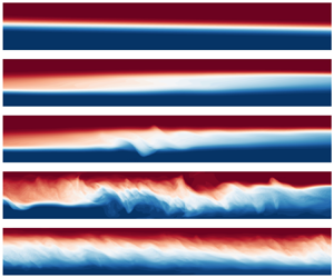
Figure 5. Snapshots of the density field in the mid-plane $y=0$ (a–e) and in the duct cross-section ( f–j) in five representative flows: (a, f) laminar (B2), (b,g) stationary wave (B5), (c,h) travelling wave (B6), (d,i) intermittent turbulence (B8, active phase) and (e,j) fully developed turbulence (B10). These cases are highlighted in bold font in table 1.

We recover, in our DNS, the same four key flow regimes (laminar, wave, intermittently turbulent and fully turbulent) identified in experimental studies of SID, in particular Meyer & Linden (Reference Meyer and Linden2014), Lefauve (Reference Lefauve2018), Lefauve et al. (Reference Lefauve, Partridge and Linden2019) and Lefauve & Linden (Reference Lefauve and Linden2020a), which is the first key result of this paper. Moreover, the DNS allow us, for the first time, to observe three-dimensional instantaneous snapshots along the entire domain, including the duct and the in- and out-flow in the reservoirs, which were not accessible to experiments. We describe each regime in turn.

4.2. Regime diagrams

In figure 6 we map the flow regimes described above in 12 DNS with the AR (figure 6a) and in 15 DNS with the BR (figure 6b) for a range of $\theta$ and $Re$.

Figure 6. Regime transitions in $\theta$–$Re$ parameter space. The large symbols are our DNS data in the (a) A-reservoir and (b) B-reservoir, and the small markers are the temperature-stratified experimental data of Lefauve & Linden (Reference Lefauve and Linden2020a) (see their figure 4e) with matched non-dimensional parameters.

These 27 DNS data points, shown as large symbols, are compared with the 148 experimental data points of Lefauve & Linden (Reference Lefauve and Linden2020a) taken from their figure 4(e) and displayed here as smaller, fainter symbols using the same colour coding for the different flow regimes. The experimental data points were obtained using the same aspect ratios ($A=30, B=1$) and with temperature stratification ($Pr\approx 7$). The regimes were identified by shadowgraph visualisation, often over a small streamwise extent of the duct (their movies can be downloaded from Lefauve & Linden (Reference Lefauve and Linden2020b)). Figure 6 therefore represents the first direct comparison of DNS results with experimental results in SID, with all non-dimensional control parameters matched.

First, we find a general agreement between DNS and experiments in the location of flow regimes in the $(\theta,{Re})$ plane, as evidenced by the fact that most large symbols (DNS) are of the same type as the smaller symbols (experiments). This is the second key result of this paper, because it confirms that our DNS, with small computationally efficient reservoirs, can reproduce the key physics of SID, encapsulated in the flow regimes.

The minor exception to this agreement is found near the L/W transition, where some of our DNS found the W regime whereas the experiments found the L regime. This may be a genuine difference, but we suspect that this may be due to the fact that the weak stationary waves found near the L transition may have been missed in the experiments. This is because the experimental shadowgraphs were visualised over a limited extent of the duct and because low-amplitude waves in low-${Re}$ temperature-stratified flows produce very small changes in refractive index and thus weak shadowgraph signals.

Second, the AR and BR yield consistent results (figure 6a,b), confirming that the smallest ‘true’ reservoir (excluding the SR for now) is indeed sufficient to reproduce the experiments. These results offer strong further support to the preliminary validation of our suite of DNS in § 3.

4.3. Shadowgraphs

We now turn to a side-by-side comparison of shadowgraph visualisations of the flow in DNS and experiments within a particular flow regime.

Experimental shadowgraph movies are obtained by the projection onto a semi-transparent screen of initially parallel light rays that have travelled through the duct along the spanwise $y$ direction. Any variations in the curvature (normal to the rays) of the density field $\rho$ (and hence refractive index field $n$) cause the rays to focus or defocus, varying the intensity that reaches the screen (Weyl Reference Weyl1954). In the limit of weak variations, the intensity of the image formed is (see e.g. Lefauve Reference Lefauve2018, § 2.1)

(4.1)\begin{equation} I(x,z,t) = \beta I_0(x,z) \int_{{-}B}^{B} (\partial_{xx}+\partial_{zz})\rho(x,y,z,t) \,{{\rm d}y}. \end{equation}

Here $\beta$ depends on $(\rho _0/n_0)\partial n/\partial \rho$ and the experimental geometry, while $I_0$ is the (approximately) uniform background intensity of the illumination. This field is thus particularly suited to detect density interfaces, and is a simple and efficient proxy to compare the structure of interfacial density waves and small-scale turbulence in DNS and experiments.

Figure 7 compares false colour instantaneous snapshots of $I(x,z)$ in the I regime over a central portion of the duct $|x|<9$. The DNS shadowgraphs reconstructed from the calculated density fields (assuming $\beta I_0 =1$) are shown in figure 7(a–c) (W3 and W5; see table 1), and the matching experimental shadowgraph images of $I/I_0$ are shown in figure 7(d–f), all at $Re=650$ and ${Pr}=7$. We show a single snapshot at $\theta =3^\circ$, at the boundary between the W and I regimes (figure 7a) and two snapshots at $\theta =5^\circ$, well into the I regime, where the flow is in a quiet laminar phase (figure 7b) and in an active turbulent phase (figure 7c). The full temporal evolution of these four shadowgraphs can be found in our supplementary movies.

Figure 7. Snapshots of shadowgraph comparing the normalised intensity $I(x,z)$ in DNS (a–c) to the matching experiments (d–f) in two cases W3 (a,d) and W5 (b,e,c, f). Magnitudes (colour bar limits) are naturally different due to the unknown experimental $\beta$ factor in (4.1). The times at which these snapshots were taken are shown by the vertical lines in the spatio-temporal diagrams of figure 8.

Figure 8. Spatio-temporal diagrams of shadowgraph in W3 (a,c) and W5 (b,d) comparing DNS (a,b) with experiments (c,d). The vertical black solid lines indicate the time of the snapshots in figure 7.

Note that these shadowgraphs were obtained in a new experimental apparatus having a wide duct $B=2$, with a regular straight rectangular section of length $A=40$. In these experiments, the reservoirs were tilted in line with the duct (the whole apparatus pivots about one end), which exactly matches the DNS. The apparatus had trumpet-shaped expansions at either end (over an additional 10 % of its length) for a smoother connection to the reservoirs. While we did not model the trumpet ends in our DNS, we used $B=2$ and the total length $A=44$ to reproduce the geometry as faithfully as possible. Trumpet ends were first used in Meyer & Linden (Reference Meyer and Linden2014) who reported no visible impact in shadowgraphs when compared to straight ends. With the parameters $A$ and $B$ increased with respect to cases B2–B10, the I regime is found at smaller $\theta$ values than would be expected from figure 6 (see Lefauve & Linden Reference Lefauve and Linden2020a).

We find good agreement in the structure of interfacial waves, somewhat reminiscent of Kelvin–Helmholtz billows, in DNS and experiments (compare figure 7a,b with figure 7d,e). These waves have higher amplitude than the stationary waves previously found in B5 (see figure 5b) because the flow is more energetic and prone to the growth of stratified shear instabilities at $B=2$ than at $B=1$, due to a weaker influence of the no-slip sidewalls (see Ducimetière et al. Reference Ducimetière, Gallaire, Lefauve and Caulfield2021, § IIIc). These waves tend to break into weak and short-lived turbulence at $\theta =3^\circ$ (placing it borderline in the I regime), and into stronger and longer-lived turbulence at $\theta =5^\circ$ (placing it well into the I regime). We also find good agreement in the overall appearance of small-scale turbulence in the ‘active’ phase (compare figures 7c and 7f). Active turbulence in the experiment extends slightly closer to the top and bottom boundaries than in the DNS. This may be a result of various factors including the non-zero thermal conductivity of the experimental duct walls, spurious reflections of light and excessive cropping of near-wall regions caused by the difficulty in locating the exact location of the walls in the shadowgraph images.

Figure 8 illustrates these temporal dynamics with the corresponding $z$–$t$ spatio-temporal diagrams in DNS (figure 8a,b) and in experiments (figure 8c,d). We find again good agreement, both in the vertical growth and decay of the waves and in the alternation and approximate period of the quiet and active phases.

These shadowgraphs show that our DNS faithfully reproduce not only the qualitative flow regimes and their distribution in $\theta$–$Re$ space, but also details of their spatial structures and temporal dynamics, which is a third key result of this paper.

5.1. Vertical profiles and gradient Richardson number

Figure 9 shows, for the five flow regimes previously shown in figure 5, the $x,y,t$-averaged velocity $\langle u \rangle (z)$, density $\langle \rho \rangle (z)$ and gradient Richardson number ${Ri}_g$ based on the gradients of these mean flows:

(5.1)\begin{equation} {Ri}_g(z)\equiv{-}{Ri}\,\frac{\partial_z \langle \rho \rangle}{(\partial_z \langle u \rangle)^2}. \end{equation}

Figure 9. Vertical profiles of the mean (a) streamwise velocity $\langle u \rangle$, (b) density $\langle \rho \rangle$ and (c) gradient Richardson number $Ri_g$ in the five flows of figure 5. We also include the I and T experimental profiles of Lefauve et al. (Reference Lefauve, Partridge and Linden2019) at $Pr\approx 700$. The vertical dashed lines in (c) denote $Ri_g=$ 0.1 and 0.25.

Such simultaneous velocity and density diagnostics are available in salt-stratified experiments (at ${Pr}\approx 700$), and we superimpose on figure 9 the mean profiles in the I and T regimes from Lefauve et al. (Reference Lefauve, Partridge and Linden2019) (their figure 4f,l). However, these diagnostics cannot be accurately obtained in temperature-stratified experiments (at $Pr\approx 7$) to match our DNS for two main reasons. First, the velocity field measurements rely on particle image velocimetry in a refractive index matched fluid, which is impossible without the introduction of another stratifying agent (necessarily having a much smaller diffusivity than temperature). Second, the density field measurements rely on laser-induced fluorescence with a dye having a much smaller diffusivity than temperature, and therefore ‘tagging’ it poorly (temperature-sensitive fluorescent dyes exist but such measurements are more difficult and less accurate).

In figure 9(a), the velocity in the L regime (B2) adopts an approximately sinusoidal profile with a low amplitude ($\max |u| \approx 0.3$), whereas in the SW, TW, I and T regimes (B5, B6, B8 and B10, respectively), the mean velocity varies nearly linearly with height for $|z|\lesssim 0.5$, and $\max |u| \approx 1$. The vertical locations of the peaks in velocity, initially around $z \approx \pm 0.5$ in the L regime, shift slightly towards the top and bottom walls $z \approx \pm 0.7$ in the I and T regimes. These observations agree qualitatively with the experimental profiles of Lefauve et al. (Reference Lefauve, Partridge and Linden2019) in the four regimes (see their figures 3f,l and 4f,l). However, exact agreement should not be expected as their $\theta$, ${Re}$ and ${Pr}$ values differ from ours.

In figure 9(b), the density profile resembles an error function in the L regime (B2) whereas it has a partially mixed layer in the W and I regimes (B5, B6, B8 and I, Exp) identified by a central region of reduced gradient (a layer) flanked by two regions of enhanced gradient (two interfaces). These three profiles are almost identical, with the nuance that the intermediate layer becomes slightly thicker from B5 to B6 to B8, as expected. Finally, in the T regime (B10 and T, Exp.), the middle layer becomes noticeably thicker, and the two interfaces flanking it become less sharp, leading to a profile approaching a uniform stratification.

In figure 9(c), the L flow has $Ri_g\approx 0.5$ throughout the central quarter of the height of the duct, flanked by steeply increasing values. The W and I flows have ${Ri}_g\approx 0.1$ near $z=0$. The T flow has a broader minimum with ${Ri}_g\approx 0.1\unicode{x2013}0.15$. The ${Ri}_g$ profiles in the I and T flows are qualitatively consistent between DNS and experiments, showing that, despite the difference in parameters, some key dynamical features of turbulence are not sensitive to the fluid properties.

Note that ${Ri}_g<0.25$ at $z=0$ in the W, I and T flows, but not in the L flow. Therefore, the mean profiles in the non-laminar flows reassuringly satisfy the Miles–Howard criterion necessary for the development of instabilities in a steady, inviscid, Boussinesq, parallel stably stratified shear flow. Moreover, in the T regime ${Ri}_g(z) \approx {Ri}_e \approx 0.1\unicode{x2013}0.15$ (i.e. robustly below the Miles–Howard criterion of 0.25). This agrees with the experimental conclusions of Lefauve & Linden (Reference Lefauve and Linden2022a) (see their figure 5), drawn from a wider dataset of 16 flows with increasing levels of turbulence. The reasons for this particular equilibrium, originally suggested by Turner (Reference Turner1973) and much observed since in numerical, experimental and observational data, are still debated. Other authors (Thorpe Reference Thorpe2010; Smyth & Moum Reference Smyth and Moum2013; Salehipour et al. Reference Salehipour, Peltier and Caulfield2018) have called it ‘self-organised criticality’ or ‘marginal stability’, and found values ranging from ${Ri}_e\approx 0.07$ to $0.25$ in various stratified shear flows that differ (sometimes significantly) from SID (Lefauve & Linden Reference Lefauve and Linden2022a).

5.2. Kinetic energy

We now study the spatio-temporal dynamics of kinetic energy along the entire length of the duct in our DNS. Similar experimental diagnostics are not yet available since the resolution of video cameras and geometry of the laser sheet limit us to shorter windows spanning only a limited part of the duct length.

We start by decomposing the velocity into mean and turbulent (fluctuating) components. Lefauve & Linden (Reference Lefauve and Linden2022b) defined the mean as the $x,t$ average. However, as our DNS data are available along the entire length of the duct, the flow (especially $u$) becomes noticeably inhomogeneous in $x$ (see figure 5a–c). A simple $x$ average would therefore make the ‘turbulent’ component artificially large by incorporating a significant non-parallel – but laminar – component. To resolve this, we define the mean and fluctuations using a moving average:

(5.2)$$\begin{gather} \bar{\boldsymbol{u}}_m\left(x,y,z,t\right)\equiv \frac{1}{\Delta L}\int_{-\Delta L/2}^{\Delta L/2}{\boldsymbol{u}\left(x-s,y,z,t\right){\rm d}s}, \end{gather}$$

(5.3)$$\begin{gather}\boldsymbol{u}^\prime_m(x,y,z,t)\equiv\boldsymbol{u}-\bar{\boldsymbol{u}}_{\boldsymbol{m}}, \end{gather}$$

and the respective ‘moving’ mean kinetic energy (MKE) and TKE are

(5.4)$$\begin{gather} \bar{k}_{m}\equiv\tfrac{1}{2}\bar{\boldsymbol{u}}_m \boldsymbol{\cdot} \bar{\boldsymbol{u}}_m, \end{gather}$$

(5.5)$$\begin{gather}k^\prime_{m}\equiv\tfrac{1}{2}\boldsymbol{u}^\prime_m \boldsymbol{\cdot} \boldsymbol{u}^\prime_m. \end{gather}$$

The length of the averaging stencil $\Delta L=10$ was chosen to maximise the time- and duct-volume-averaged MKE $\langle \bar {k}_{m}\rangle _{\mathcal {V},t}$, as shown in figure 10(d).

Figure 10. Snapshots of DNS B6 at $t=160$ showing the (a) density, (b) moving-averaged TKE $k^\prime _m$ defined in (5.5) and (c) ‘naive’ TKE based on $\boldsymbol {u}'=\boldsymbol {u}-\langle \boldsymbol {u}\rangle _{x,t}$. (d) Bulk MKE $\langle \bar {k}_m \rangle _{\mathcal {V},t}$ as a function of the stencil length $\Delta L$. The dashed line corresponds to our choice in the remainder of the paper $\Delta L=10$.

In figure 10(a–c) we demonstrate the use of this moving average with a snapshot in the travelling wave regime (B6, as in figure 5c). The underlying turbulence ‘hotspots’ visualised by the density field (figure 10a) are faithfully captured by our moving-averaged TKE $k^\prime _{m}$ (figure 10b), whereas they are greatly overestimated by the ‘naive’ TKE based on the $x,t$-averaged velocity (figure 10c), which is equivalent to setting $\Delta L=2A=60$ and $x=0$ in (5.2).

Figure 11 shows time series of the duct-volume-averaged MKE $\langle \bar {k}_{m} \rangle _\mathcal {V}$ (figure 11a) and TKE $\langle k^\prime _{m} \rangle _\mathcal {V}$ (figure 11b) for the five regimes shown in figure 5. The laminar (B2) and the stationary wave (B5) cases quickly reach a steady state with constant or near-constant MKE (figure 11a) and zero or near-zero TKE (figure 11b). We note that the flow in B5 is faster than in B2 as their MKE plateau at $\approx$0.2 and $\approx$0.06, respectively. The travelling wave (B6) case shows more fluctuations in the MKE (but also $\approx$0.2), and a larger TKE fluctuating between $\approx$0.001 and 0.005. The intermittent and turbulent cases (B8 and B10) show much larger fluctuations in MKE and TKE, and a significantly larger TKE than in the travelling wave case. In these two cases, the MKE and TKE fluctuations are of comparable magnitude to their temporal mean. The TKE fluctuations are particularly striking, showing that the flow, even when averaged over the entire duct volume, is alternating between phases of intense and weak turbulence. These fluctuations appear to be quasi-periodic with a period of $\approx$100 ATU, corresponding to approximately one-and-a-half full-duct transit times at advective speed 1. Although long known from experiments, the mechanisms responsible for these fluctuations remain poorly understood and beyond the scope of this paper. The intermittent regime (B8) differs from the turbulent regime (B10) in that its TKE occasionally drops to zero for extended periods of time (here $150\lesssim t \lesssim 210$); i.e. the flow relaminarises in the duct. This never happens in the turbulent regime, although it does feature cycles of weaker and stronger turbulence.

Figure 11. Time series of volume-averaged (a) MKE and (b) TKE for the five cases B2–B10 of figure 5. A snapshot of density and TKE in B6 at $t=160$ is shown in figure 10(a,b).

Our MKE and TKE time series are approximately similar to their salt-stratified experimental counterparts in Lefauve & Linden (Reference Lefauve and Linden2022b) (see their figures 1(a,b) and 3( f,i,o,r), noting that they correspond to $Pr\approx 700$). This agreement between the DNS and experiments extends from the values of MKE $\approx$0.2 in the W/I/T regimes to the mean TKE $\approx 0.01\unicode{x2013}0.02$ in the I/T regimes, corresponding to a typical turbulent/mean velocity ratio of $\sqrt {k^\prime _m/\bar {k}_m} \approx 20\,\%\unicode{x2013}30$ % (although the ratio appears to be slightly higher in the DNS B10 than in the experiments T2 and T3). The large temporal fluctuations in B10 (which is at the limit of our computational resources) are typical of a flow near the I/T regime transition rather than well into the T regime, as was already clear from its location on the regime diagram (figure 6b). The experimental time series of TKE (see Lefauve & Linden (Reference Lefauve and Linden2022b), figure 3(o,r) in their datasets T1 and T3) suggest that these temporal fluctuations would significantly decrease in a more highly turbulent flow at higher ${Re}$ and $\theta$ (i.e. that the TKE would become increasingly steadily sustained at a higher level). Our B8 has a time series similar to their dataset T1 (both being near the I/T transition), whereas their more turbulent dataset T3 is further away from the I/T transition.

Our MKE and TKE time series are generally out of phase in the I and T regimes (figure 11), although the negative correlation is less clear in the T regime. In other words, in B8, the MKE tends to decrease as the TKE increases (i.e. turbulence slows down the mean flow), and vice versa (the MKE tends to increase when the TKE decreases or is zero). This behaviour, wherein the mean flow and the turbulence appear to regulate one another, supports the ideas of ‘self-organised criticality’ and ‘marginal stability’ discussed previously. In B10, this negative correlation holds until $t\approx 200$, at which point the TKE increases rapidly while the MKE continues increasing, leading both TKE and MKE to peak approximately at the same time. In the T regime the mean flow thus appears closer to a turbulent threshold, such that perturbations grow more readily without ‘waiting’ for the mean flow to fully accelerate. Equivalently, in the T regime (which has the highest $\theta \,{Re}$), the mean flow is able to keep accelerating despite the growing turbulence, presumably due to a higher forcing (because it is proportional to $\theta$) and a lower TKE dissipation than in the I regime (because it is inversely proportional to ${Re}$) .

Finally, figure 12 shows $x$–$t$ diagrams of TKE (averaged along $y$ and $z$) for B2 to B10 (left to right) after the initial transients have decayed ($t>80$). In the L regime (B2, figure 12a), the TKE is negligible except very near the ends of the duct $|x|\approx 30$, where tiny fluctuations are found where the exchange flow discharges into the reservoirs. In the stationary W regime (B5, figure 12b), the TKE at both ends is higher, extends a little further into the duct and is also occasionally visible near the centre of the duct $|x|\approx 0$ where it appears to remain stationary. Similarly, the ‘end waves’ do not propagate into the duct and may be swept into the reservoirs, implying that their phase speed is smaller than the convective speed of the flow (i.e. that the flow may be critical or supercritical in these regions).

Figure 12. Spatio-temporal diagram of TKE $\langle k^\prime _m \rangle _{y,z}(x,t)$ for $t\in [80, 260]$ (after the initial transients) in DNS (a) B2, (b) B5, (c) B6, (d) B8 and (e) B10. Note the colourbar is in log scale.

In the travelling W regime (B6; figure 12c), larger TKE develops and it sometimes appears to propagate along the duct. These waves appear to be generated within the duct rather than travelling from the ends. In the I regime (B8, figure 12d), a laminar phase develops between $120 \lesssim t \lesssim 220$, lasting over a full duct transit time (taking ${\approx }2A=60$ ATU at the maximum flow speed $\approx$1). The boundary between laminar and turbulent phases appears to propagate from one end of the duct to the other. In the T regime, a quiescent patch develops near the centre of the duct just after $t=200$. The quiescent phase ends when energetic turbulent regions move in from both ends of the duct.

5.3. Pressure

We now analyse the pressure field throughout the interior of the duct, which is inaccessible to experiments.

Figure 13 shows representative snapshots of the spanwise-averaged pressure $\langle p \rangle _y$ and five equally spaced isopycnals for B2, S6, B6, S8 and B8. Note that our definition of the non-dimensional density $\rho$ as the perturbation around the reference $\rho _0$ (see § 2.1) implicitly subtracts the hydrostatic pressure due to $\rho _0$ in the reservoirs. The pressure distribution is qualitatively similar in the W and I regimes (S6, B6, S8, B8; figure 13b–e), but different in the L regime (B2; figure 13a).

Figure 13. Spanwise-averaged pressure field snapshots (colours) superimposed with five isopycnals (lines) $\rho =0,\pm 0.4, \pm 0.8$ in DNS (a) B2, $t=100$, (b) S6, $t=108$, (c) B6, $t=108$, (d) S8, $t=235$ and (e) B8, $t=250$.

In the L flow inclined at $\theta =2^\circ$ (figure 13a), the pressure conforms to what we expect from an exchange flow in a horizontal duct where $\theta$ does not play a major role (see the sketch in Lefauve (Reference Lefauve2018), figure 1.4). Essentially, each layer experiences a favourable streamwise pressure gradient: $-\partial _x p > 0$ in the right-flowing lower layer where $u>0$, causing a convective acceleration along the duct, $u \partial _x u >0$; and vice versa, $-\partial _x p < 0$ in the left-flowing upper layer where $u<0$, causing the expected $u \partial _x u <0$ ($\partial _x u >0$ in both layers). This is achieved by a high-pressure zone in the bottom left and top right reservoirs (in red), and a low-pressure zone in the top left and bottom right reservoirs (in blue), as would be naturally obtained by the hydrostatic equilibrium of two solutions having different densities and required to match hydrostatic pressures at mid-height.

However, in flows inclined at $\theta =6^\circ$ and $8^\circ$ (figure 13b–e), the pressure has a large-scale global minimum in the centre of the duct (in blue). This low-pressure zone causes both layers to experience a favourable pressure gradient over approximately the first half of their course, causing the fluid to accelerate as it flows towards the centre of the duct, but an adverse pressure gradient over the second half of their course, causing the fluid to decelerate from the centre of the duct as it flows away from the centre of the duct. This adverse pressure gradient confirms the predictions of Lefauve & Linden (Reference Lefauve and Linden2022a) (see their § 4.3) who, without having direct access to the pressure field, found that in most datasets the Reynolds-averaged budget implied the existence of an adverse pressure gradient.

Furthermore, these features of the pressure distribution are found in both the BR and SR geometries (compare figures 13(b,c) and 13(d,e), despite the difference in the location of the low-pressure region in the I cases) as the outflowing layers must decelerate in both geometries. In the BR (and by extension in AR and benchmark), this occurs since the streams encounter fluid at rest in a large reservoir; in the SR, this occurs since the streams encounter the artificial forcing region where the flow is brought to rest. This suggests that the SR cases appear to qualitatively mimic the benchmark case despite the absence of reservoirs, which may help reduce computational costs further in future studies.

Finally, we address the impact of the adverse pressure gradient on the density field and its interface(s). The isopycnals in figure 13(a–d) (the yellow lines denoting the lower, densest layer, and the dark blue lines denoting the upper, lightest layer) show that the central low-pressure zone coincides with an increasing depth of each layer in the direction of flow. This is expected from mass conservation along a straight duct: an accelerating layer (because of a favourable pressure gradient or gravitational forcing) must become thinner along its course, and vice versa, a decelerating layer (caused by an adverse pressure gradient) must become thicker. We also see from the isopycnals that this thickening coincides with the emergence of displaced isopycnals (in B6, S6) and turbulence (in B8, S8). Note that this interface thickening implies the occurrence of internal hydraulic ‘jump’ and the set-up of hydraulic control (Meyer & Linden Reference Meyer and Linden2014; Lefauve & Linden Reference Lefauve and Linden2020a) in the middle of the duct. This effect of internal hydraulics is beyond the scope of this paper and will be revisited in more detail in our future work.

5.4. Turbulent energy fluxes

We conclude this section with an analysis of the turbulent energy fluxes in datasets B5, B6, B8 and B10 and use it to demonstrate how DNS data allow us to overcome the current experimental limitations identified in Lefauve & Linden (Reference Lefauve and Linden2022b) (their Appendix B) and improve our physical understanding of stratified turbulent mixing.

To do so, we adopt the ‘shear-layer’ non-dimensional framework of Lefauve & Linden (Reference Lefauve and Linden2022a) (§ 3.3) by rescaling all velocities such that the $(x,t)$-averaged $\langle u \rangle _t(y=0,z)$ has extrema $\pm 1$, and rescaling all spatial variables such that the $z$ locations of these extrema are located at $\pm 1$ (whereas previously the top and bottom walls were located at $\pm 1$); we call this central region of non-dimensional height $=2$ the shear layer. This rescales the effective Reynolds number and bulk Richardson number of the flow, which we now denote $Re^s$ and $Ri_b^s$, respectively, and allows for more meaningful comparison of datasets with one another as well as with the literature. Following Lefauve & Linden (Reference Lefauve and Linden2022a) we further remove from our analysis all data outside the shear layer, i.e. exclude the top and bottom near-wall boundary layers in $z$, as well the boundary layers in $y$ (where the peak $|u|$ is less than 0.7), in order to focus on the ‘core’ region with turbulent activity.

We then define the non-dimensional time- and volume-averaged MKE $\bar {K} = \langle \bar{k}_m \rangle _\mathcal {S}$ and TKE $K' = \langle k'_m \rangle _\mathcal {S}$, as well as the mean scalar variance $\bar {K}_\rho \equiv Ri^b_s \langle \bar {\rho }_m^2 /2 \rangle _\mathcal {S}$ and turbulent scalar variance $K_\rho ' \equiv Ri^b_s \langle \rho '_m{}^2 /2 \rangle _\mathcal {S}$. Note that the subscript $m$ denotes the moving average introduced in § 5.2, and that the multiplying factor $Ri_b^s$ allows us to interpret $K_\rho,K_\rho '$ as proxies for potential energy under linear stratification. The simple bracket averaging $\langle \cdot \rangle _\mathcal {S}$ denotes a combined three-dimensional volume averaging over the shear-layer region and along the central two-thirds of the duct (by excluding one averaging window $\Delta L$ on either end) and time averaging over $t\in [80, 280]$ (focusing on the established dynamics as in figure 12).

Considering the evolution equations of these four energy reservoirs under a set of ‘safe’ approximations in SID, Lefauve & Linden (Reference Lefauve and Linden2022b) derived the following approximate balances between energy fluxes in a statistically steady state:

(5.6a)$$\begin{align}\mathcal{P} &\approx \mathcal{F} - \bar{\epsilon} \,\quad \text{(production of } K' = \text{forcing} - \text{laminar dissipation)}, \end{align}$$

(5.6b)$$\begin{align}\mathcal{E} &\approx \mathcal{P} - \mathcal{B} \quad \text{(dissipation of } K' = \text{production} - \text{buoyancy flux)}, \end{align}$$

(5.6c)$$\begin{align}\mathcal{P}_\rho &\approx \varPhi^{\bar{K}_\rho} \quad\quad \text{(production of } K'_\rho = \text{boundary net flux of unmixed fluid)}, \end{align}$$

(5.6d)$$\begin{align}\chi &\approx \mathcal{P}_\rho \ \ \quad\quad \text{(dissipation of } K'_\rho \text{ i.e. mixing} = \text{production)}, \end{align}$$

where the eight fluxes are

(5.7)\begin{gather} \left.\begin{gathered} \mathcal{P} \equiv{-} \langle u'v'\partial_y \bar{u}+ u'w' \partial_z \bar{u} \rangle_\mathcal{S}, \quad \mathcal{F} \equiv Ri_b^s \sin \theta \langle \bar{u}\bar{\rho}\rangle_\mathcal{S} , \\ \bar{\epsilon} \equiv \frac{2}{Re^s} \langle||\bar{\textsf{\textit{\textbf{s}}}}||^2\rangle_\mathcal{S}, \quad \mathcal{E} \equiv \frac{2}{Re^s} \langle ||{\boldsymbol{\mathsf{s}}}'||^2 \rangle_{\mathcal{S}}, \end{gathered}\right\} \end{gather}

(5.8)\begin{gather} \left.\begin{gathered} \varPhi^{\bar{K}_\rho} \equiv{-}Ri_b^s \left\langle \frac{\left.\left( u\dfrac{\rho^2}{2}\right)\right|^{x^+}_{x^-}}{x^+{-} x^-} \right\rangle_\mathcal{S}, \quad\mathcal{B} \equiv Ri_b^s \langle w' \rho' \rangle_\mathcal{S}, \\ \mathcal{P}_\rho \equiv{-} Ri_b^s \langle w' \rho' \partial_z \bar{\rho} \rangle_\mathcal{S}, \quad \chi \equiv \frac{Ri_b^s}{Re^s \, Pr}\langle |\boldsymbol{\nabla} \rho'|^2\rangle_\mathcal{S}, \end{gathered}\right\} \end{gather}

where $\bar {{\boldsymbol{\mathsf{s}}}}, {\boldsymbol{\mathsf{s}}}'$ are the strain rate tensors of the mean and turbulent velocity fields, respectively. From (5.7) and henceforth we omit the subscripts $m$, using the moving average in all bar and prime quantities. Equations (5.6b) and (5.6d) are the classical balances of Osborn (Reference Osborn1980) and Osborn & Cox (Reference Osborn and Cox1972), respectively, while (5.6a) and (5.6c) are specific to SID: the mean kinetic energy is sustained through $\mathcal {F}$ by the gravitational acceleration and the mean scalar variance is sustained through $\varPhi ^{\bar {K}_\rho }$ by the inflow of unmixed fluids from the reservoirs into the volume of interest.

Figure 14(a–d) demonstrates how closely the four balances (5.6a–d) hold in DNS, where the thick diagonal solid line denotes equality between the left-hand side (vertical axis) and right-hand side (horizontal axis) of each equation. The open symbols in figure 14(a,b,d) denote the value of the left- and right-hand side exactly as in (5.6a,b,d), and are generally in balance, except in a few cases. In these few cases, the balance is improved by the filled symbols obtained after adding the following boundary fluxes:

(5.9a)\begin{align} \varPhi^{\bar{K}} &\equiv{-} \left\langle \frac{\left.\left(u \left(\dfrac{{\boldsymbol{u}}^2}{2}+p\right)\right)\right|^{x^+}_{x^-}}{x^+{-} x^-} \right\rangle_{\mathcal{S}}\ \text{to the right-hand side of } {(5.6a)},\end{align}

(5.9b)\begin{align} \varPhi^{K'} &\equiv{-} Ri_b^s \left\langle \frac{\left.\Biggl(u' \Biggl(\dfrac{{\boldsymbol{u}'}^2}{2}+p'\Biggr)\Biggr)\right|^{x^+}_{x^-}}{x^+{-} x^-} + \dfrac{\left.\Biggl(v' \Biggl(\dfrac{{\boldsymbol{u}'}^2}{2}+p'\Biggr)\Biggr)\right|^{y^+}_{y^-}}{y^+{-} y^-} \right.\nonumber\\ &\quad \left. + \dfrac{\left.\Biggl(w' \Biggl(\dfrac{{\boldsymbol{u}'}^2}{2}+p'\Biggr)\Biggr)\right|^{z^+}_{z^-}}{z^+{-} z^-} \right\rangle_\mathcal{S} \ \text{to the right-hand side of } {(5.6b)}, \end{align}

(5.9c)\begin{align} \varPhi^{K'_\rho} &\equiv{-} Ri_b^s \left\langle \frac{\left.\left(u'\dfrac{\rho' {}^2}{2}\right)\right|^{x^+}_{x^-}}{x^+{-} x^-} + \frac{\left.\left(v' \dfrac{\rho'{}^2}{2}\right)\right|^{y^+}_{y^-}}{y^+{-} y^-} \right.\nonumber\\ &\quad \left. + \frac{\left.\left(w' \dfrac{\rho'{}^2}{2}\right)\right|^{z^+}_{z^-}}{z^+{-} z^-} \right\rangle_\mathcal{S} \text{to the right-hand side of } {(5.6d)},\end{align}

where $x^\pm, y^\pm, z^\pm$ are the edges of our shear-layer averaging domain, and we neglected in (5.9a) the spanwise and vertical mean transport, in (5.9a)–(5.9b) the work of viscous forces and in (5.9c) the transport by molecular diffusion, in order to focus on the dominant contributions. The fact that these fluxes improve the balance only slightly demonstrates that they can, to a reasonable approximation, be neglected in SID energetics. This result was hypothesised in Lefauve et al. (Reference Lefauve, Partridge and Linden2019) and Lefauve & Linden (Reference Lefauve and Linden2022b) but their experiments could not clearly confirm it due to excessive noise in the computation of (5.9) and the lack of the pressure. After correction, the only remaining discrepancy is found in $\chi$ in the most turbulent flow B10 (figure 14d), where it is $33\,\%$ below the expected value to balance $\mathcal {P}_\rho$.

Figure 14. Correlation between some of the time- and volume-averaged energy fluxes (5.7)–(5.8) in B5, B6, B8 and B10. (a–d) Verification of the energy balances in (5.6) (left-hand side versus right-hand side), filled symbols denoting the minor correction of boundary fluxes (5.9). (e, f) Verification of the empirical relations (5.10). (g) Determination of the empirical flux coefficient (5.11) suggesting $\varGamma =0.1$.

Part of this discrepancy ($13\,\%$ out of $33\,\%$) is explained by our neglect of molecular diffusion $Ri_b^s/(Re^s Pr)|\boldsymbol {\nabla }\bar {\rho }|^2$ in (5.6d), which at these values of $Re^s$ and $Pr$ is ‘only’ a factor of five smaller than $\chi$. The remaining $20\,\%$ of this discrepancy is most likely be due to under-resolution, as we explain next. Our spatial grid in B10 approaches the time- and volume-averaged Batchelor length scale computed in the shear layer $[\Delta x, \Delta y, \Delta z] = [3.3, 2.3, 2.3] \, \ell _B$, where $\ell _B \equiv \mathcal {E} ^{-1/4}(Re^s)^{-3/4}Pr^{-1/2}= 0.01$ in non-dimensional shear-layer units. We verified that $\chi$ was nearly identical on the coarser grid (by a factor of $\approx$2 in $x$ and $y$; see table 1). However, the time series of the volume-averaged $\mathcal {E}$ undergoes cycles (much like the TKE in figure 11b) with peaks being three times larger than the time average used for $\ell _B$. Using this peak value, our grid only resolves $\approx [4, 3, 3] \, \ell _B$, which may be too coarse to capture the entire spectrum of $\boldsymbol {\nabla }\rho '$ during the most turbulent events. This should be kept in mind for future DNS which aim to fully resolve mixing.

Having largely verified (5.6), we now examine in figure 14(e, f) two robust empirical relations from the SID experimental literature in very turbulent flows ($\mathcal {E} \gg \bar {\epsilon }$):

(5.10a)$$\begin{gather} \mathcal{P_\rho} \approx \mathcal{B} \quad \text{because } \partial_z \langle \rho\rangle_{x,t} \approx{-}1 \text{ in the the shear layer}, \end{gather}$$

(5.10b)$$\begin{gather}\mathcal{E} + \bar{\epsilon} \approx \mathcal{E} \approx 0.035 \theta \quad \text{because of hydraulic control and } Ri^b_s \approx 0.10\unicode{x2013}0.15, \end{gather}$$

where $\theta$ is in radians (Lefauve & Linden Reference Lefauve and Linden2022b). Our DNS data generally confirm (5.10a) (figure 14e) and (5.10b) (figure 14f) but with two reservations. First, in B10, $\mathcal {P}_\rho$ is $25\,\%$ below the expected value $\mathcal {B}$ as a result of the mean vertical density gradient being slightly weaker in our DNS (at $Pr=7$) than in the experiments (at $Pr=700$). Second, although the total dissipation $\mathcal {E}+\bar {\epsilon }$ corrected with the appropriate boundary fluxes (filled symbols) follows (5.10b) (in particular since our $Ri_b^s$ indeed converges to 0.12–0.14 in all datasets B5–B10), the agreement is less good for the turbulent dissipation alone $\mathcal {E}$ (smaller open symbols). In other words, our ability to fully capture $\mathcal {E}$ and all boundary fluxes in DNS allows us to quantify the relative importance of the (subdominant) terms $\varPhi ^{\bar{K}},\varPhi ^{K'}$ and $\bar {\epsilon }$ in SID energetics. We hypothesise that stronger turbulence at higher values of $\theta \,Re^s$ would see these subdominant terms plateau, and that $\mathcal {E}$ would follow $0.035 \theta$ increasingly closely.

We now move to the ultimate goal of this energetics analysis, and more broadly of research into turbulent mixing, which is to eventually connect all turbulent fluxes to known non-dimensional parameters of the flow in a closed system of equations. In the asymptotic ‘strong SID turbulence’ scenario under which $\bar {\epsilon }$ becomes subdominant, we have seven key turbulent fluxes in (5.7), (5.8) and six independent equations: the four equations (5.6) expressing conservation of energy, and the two robust empirical equations (5.10), one of which crucially involves the single input parameter $\theta$. To close the system, we require a seventh independent equation, which we choose to be the classical flux parameter in the ocean mixing literature:

(5.11)\begin{equation} \varGamma \equiv \frac{ \mathcal{B} }{\mathcal{E}}. \end{equation}

Combining these seven equations in matrix form, and inverting this linear system, we deduce all fluxes in closed form as

(5.12) \begin{align} &\begin{bmatrix} 1 & -1 & 0 & 0 & 0 & 0 & 0 \\ 0 & -1 & 1 & 1 & 0 & 0 & 0 \\ 0 & 0 & 0 & 0 & 1 & -1 & 0 \\ 0 & 0 & 0 & 0 & 1 & 0 & -1 \\ 0 & 0 & 0 & 1 & -1 & 0 & 0 \\ 0 & 0 & 1 & 0 & 0 & 0 & 0 \\ 0 & 0 & \varGamma & -1 & 0 & 0 & 0 \\ \end{bmatrix} \begin{bmatrix} \mathcal{F} \\ \mathcal{P} \\ \mathcal{E} \\ \mathcal{B} \\ \mathcal{P}_\rho \\ \varPhi^{\bar{K}_\rho} \\ \chi \end{bmatrix} = \begin{bmatrix} 0 \\ 0\\ 0 \\ 0\\ 0\\ 0.0035\theta \\ 0 \end{bmatrix} \nonumber\\ &\quad \Longrightarrow\ \begin{bmatrix} \mathcal{F} \\ \mathcal{P} \\ \mathcal{E} \\ \mathcal{B} \\ \mathcal{P}_\rho \\ \varPhi^{\bar{K}_\rho} \\ \chi \end{bmatrix} = 0.035\theta \begin{bmatrix} 1+\varGamma \\ 1+\varGamma \\ 1 \\ \varGamma \\ \varGamma \\ \varGamma \\ \varGamma \end{bmatrix} . \end{align}

This expression highlights the importance of knowing the value of $\varGamma$, and its potential dependence on any of the non-dimensional flow parameters such as $\theta, Re$ or $Pr$, as the keystone to turbulent mixing in SID. Figure 14(g) shows $\mathcal {B}$ versus $\mathcal {E}$ (both of which are fully resolved in our DNS) which strongly supports the constant value of $\varGamma \approx 0.1$ in the two most turbulent datasets (0.097 and 0.096 in B8 and B10, respectively). The experimental data Lefauve & Linden (Reference Lefauve and Linden2022b) also found $\varGamma \approx 0.1$ but their insufficient spatial resolution to fully capture $\mathcal {E}$ led them to conjecture a slightly lower value in the range 0.05–0.07. Our DNS allow us to confirm that $\varGamma \approx 0.1$ is a robust estimate, at least for turbulence at $Pr=7$ in this narrow region of the $(\theta,Re)$ space. This value is smaller than the classical $\varGamma \approx 0.2$ found in most of the literature, potentially because of the shear-driven nature of SID turbulence, sustained by gravitational forcing, inducing a different type of equilibrium from that in other canonical flows.