


1. Introduction
A long-standing challenge in turbulence is viable theories for canonical turbulent shear flows such as jets, wakes and mixing layers, as well as turbulent boundary layers, and their characterization in terms of scaling laws and possible flow invariances. As turbulent shear flows are prevalent in numerous natural and industrial contexts, the importance of constructing viable jet theories cannot be overstated.
The incompressible plane jet is a paradigm flow for understanding laminar and turbulent shear flow phenomena. Here, we investigate turbulent plane jets (TPJs), aiming towards a more accurate theory for them.
Lie symmetry analysis (LSA) is a powerful method that has found widespread applications in physics, fluid mechanics and other areas of science; see Cantwell (Reference Cantwell2002). It is a general method for analysing functions and systems of differential equations, and is essential in developing our theory from which new jet scaling laws and other consequences will emerge.
The jet with steady bulk velocity  $U_0$ enters a domain of the same fluid normal to a flat wall at
  $x=0$ through a slit of width
  $H$. The Cartesian coordinates
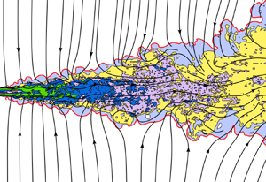
  $(x,y,z)$ respectively denote the streamwise, transverse (lateral) and spanwise directions. Figure 1 sketches the mean flow and mean streamlines in the TPJ, and figure 2 shows an instantaneous flow from direct numerical simulations (DNS) at Reynolds number
 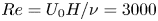 $Re=U_0H/\nu =3000$, where
  $\nu$ is the kinematic viscosity. Note that the near field in figure 2 would be different if it were initially a laminar inlet flow condition; however, the region further downstream looks similar to an initially laminar jet.

Figure 1. A TPJ emerging from a wall: mean flow and streamlines.

Figure 2. Cross-sectional view of plane jet DNS emanating from a fully turbulent channel flow at Reynolds number  $Re=3000$, showing external, entraining flow streamlines entering the jet through the turbulent–non-turbulent interface (red line). Zones of green, dark blue, purple, yellow and light blue show regions of progressively decreasing vorticity. (Some streamlines are discontinued to avoid overcrowding.)
Most theories involve free unconfined jets, i.e. without any confining boundaries in  $x$,
$x$,  $y$ or
  $z$, and irrotational external fluid being entrained into the turbulent jet. In practice, however, no laboratory facility involves the total exhaust of the turbulent jet flow out of the laboratory; the entraining flow is re-circulated from downstream back upstream towards the jet inlet, and hence is weakly vortical – called the back-flow. Otherwise, the entraining flow must be supplied externally to the jet inflow, typically assumed to be irrotational.
Because the density is constant, it is convenient in the ensuing analysis to subsume the density with the pressure, i.e. henceforth, we designate the kinematic pressure (or just ‘pressure’ for short) to be  $p={\rm pressure}/{\rm density}$. The Reynolds decomposition of the flow is
  $\boldsymbol {u}(x,y,z,t)=\boldsymbol {U}(x,y)+\boldsymbol {u}'(x,y,z,t)$, where
  ${\boldsymbol {u}}(x,y,z)=\langle u,v,w\rangle (x,y,z)$ is the velocity field,
  ${\boldsymbol {U}}(x,y)=\langle U,V,0\rangle (x,y)$ is the mean velocity field with
  $U=\bar {u}$ and
  $V=\bar {v}$ – where the overbar denotes the average in time and in
  $z$ because of the spanwise statistical homogeneity – and
  $\boldsymbol {u}'(x,y,z,t)$ is the fluctuating velocity field, with
  $\overline {u'}=\overline {v'}=\overline {w'}=0$. The centreline streamwise mean velocity is
  $U_c (x)= U(x,y=0)$. Similarly, the pressure field is
  $p(x,y,z,t) =P(x,y)+p'(x,y,z,t)$, where
  $P(x,y)=\bar {p}$ is the mean pressure field,
  $p'(x,y,z,t)$ is the fluctuating pressure field, with
  $\overline {p'}=0$, and
  $P_c(x)=P(x,y=0)$.
A commonly used characteristic length, the jet half-width  $b(x)$, is defined as the transverse distance from the centreline to where the mean streamwise velocity is
  $U_c(x)/2$. We note that whereas in the laminar plane jet the half-width
  $b(x)$ grows as
  $\sim x^{2/3}$ (Schlichting & Gersten Reference Schlichting and Gersten2003), the TPJ (which exists at high Reynolds number) grows like
  $\sim x^1$ in the far field in classical analysis (Pope Reference Pope2000).
The TPJ has three distinct flow regions: the near field, the intermediate field, and the far field. The near field is in the range  $0\lesssim x/H\lesssim 5$; note that the initial shear layers can be laminar, transitional or turbulent, i.e. emanating from a fully turbulent channel. Flow instabilities in the intermediate region
  $5\lesssim x/H\lesssim 20$ lead to fully three-dimensional turbulence, progressively achieving self-preservation downstream in the far field,
  ${x/H\gtrsim 20}$. Here, we focus on the far field, although insights pertaining to the first two regions will also emerge from our analysis.
In classical analysis, incompressible plane laminar and turbulent jets are assumed to be thin – that is, the jet width is much less than the corresponding streamwise distance,  $b(x)\ll x$, and the jet span. Hence the boundary layer approximation is applied in which almost all streamwise gradients of flow variables are considered small and are neglected, whence the transverse momentum equation leads to
  $\partial P/\partial y \approx 0$, i.e. the flow is almost isobaric and therefore the pressure is constant in the entire flow domain. But, as we will see in the next section, some experiments contradict this assumption.
For the ensuing analysis, we define the non-dimensional mass flux  $Q_m(x)$ per unit span as
 \begin{equation} Q_m(x) = \frac{1}{Q_0}\int_{-\infty}^{\infty} \rho\,U(x,y)\, {{\rm d}y}, \end{equation}
where  $Q_0= \int _{-\infty }^{\infty } \rho \,U(0,y) \,{{\rm d}y}$ is the inlet mass flux per unit span. And three non-dimensional streamwise momentum fluxes – the total momentum flux
  $J_T$, the momentum flux of the streamwise mean flow
  $J_U$, and the mean momentum flux due to the turbulence
  $J_u$ – are defined as
 $$\begin{gather} J_U(x) \equiv \frac{1}{J_{T0}}\int_{-\infty}^{\infty} \rho\,U^2(x,y) \,{{\rm d}y}, \end{gather}$$
 $$\begin{gather}J_u(x) \equiv \frac{1}{J_{T0}}\int_{-\infty}^{\infty} \rho\,\overline{u'^2}(x,y)\,{{\rm d}y}, \end{gather}$$
 $$\begin{gather}J_T(x) \equiv \frac{1}{J_{T0}}\int_{-\infty}^{\infty} \rho (U^2+\overline{u'^2})(x,y) \,{{\rm d}y} = J_U(x)+J_u(x), \end{gather}$$
where  $J_{T0}=\int _{-\infty }^{\infty } \rho (U^2+\overline {u'^2})(0,y) \,{{\rm d}y}$ is the inlet total momentum flux per unit span. We have
  $J_U\gg J_u$ (because
  $U^2\gg \overline {u^{'2}}$).
Our goal is first to identify the shortcomings in classical jet theory. Second, we develop a new TPJ theory, based on more realistic physical principles, that predicts and explains the experiments, overcoming the shortcomings of prior TPJ theories. We achieve this by applying a more accurate boundary layer approximation to jets, and then applying LSA to the governing equations. Finally, we will articulate and emphasize the need for much more carefully designed and accurately measured jet flows, as well as highly resolved high Reynolds number jet simulations.
The rest of the paper is organized as follows. In § 2, we identify some of the outstanding problems in current jet theories, and establish a condition on momentum flux that all jets must satisfy. In § 3, we apply LSA to the TPJ equations to derive new scaling laws. Predictions, validations and other results from our new theory are presented against measurements in § 4. We summarize our findings in § 5.
2. Improving the boundary layer approximation in jets
In our theory, the most important new physical idea is that the jet is not truly ‘thin’ in the classical sense, hence the application of the classical boundary layer approximation to jets is questionable.
In statistically steady incompressible high Reynolds number TPJs, viscous effects are negligible, and the mean mass, momentum and turbulent kinetic energy (TKE) balance equations are (Pope Reference Pope2000)
 $$\begin{gather} \frac{\partial U}{\partial x} + \frac{\partial V}{\partial y} = 0, \end{gather}$$
 $$\begin{gather}\frac{\partial (U^2+\overline{u'^2}+P)}{\partial x} + \frac{\partial (UV+\overline{u'v'})}{\partial y} = 0, \end{gather}$$
 $$\begin{gather}\frac{\partial (UV+\overline{u'v'})}{\partial x} + \frac{\partial (V^2+\overline{v'^2}+P)}{\partial y} = 0, \end{gather}$$
 $$\begin{gather}U\,\frac{\partial k}{\partial x} + V\,\frac{\partial k}{\partial y} ={-}{\frac{\partial \overline{v'(u'^2+v'^2+w'^2+p')}}{\partial y}} - {\overline{u'v'}}\,\frac{\partial U}{\partial y} - \epsilon = T +P_r + \epsilon, \end{gather}$$
with boundary conditions,
 \begin{equation} \left.\begin{gathered} \hbox{at } y=0 , \quad U=U_c(x), \quad V=0, \quad \dfrac{{\rm d}U}{{\rm d}y}=0, \quad -\overline{u'v'}=0,\\ \hbox{at } y={\pm} \infty , \quad U=0, \quad P=P_\infty, \quad -\overline{u'v'}=0, \end{gathered}\right\}\end{equation}
where  $k=(\overline {u'^2}+\overline {v'^2}+\overline {w'^2})/2$ is the TKE (per unit density), and
  $\overline {u'^2}$,
  $\overline {v'^2}$ and
  $\overline {w'^2}$ are the variances of the turbulent velocity fluctuation components. The left-hand side of (2.4) is the convective transport of TKE, and on the right-hand side are
  $T$, the turbulent diffusion of TKE,
  $P_r= -\overline {u'v'}\,({\partial U}/{\partial y})$, the production of TKE due to the mean velocity gradients, and the dissipation
  $\epsilon$. (A second term in
  $P_r$, namely
  $-(\overline {u'^2}-\overline {v'^2})\,\partial U/\partial x$, is small and we ignore it here.)
Some experiments (figure 3a) show that  $\partial P/\partial y\not =0$ – contradicting classical theory. Hence initially we will consider all terms in (2.2) and (2.3), then remove only those terms that we can prove to be negligible. Townsend (Reference Townsend1976) appears to have been the first to have noted that the transverse gradient of the mean static pressure may not necessarily be negligible. Unfortunately, his theoretical note has been largely ignored; however, as delineated throughout this paper,
  $\partial P/\partial y$ is important.

Figure 3. Profiles of: (a) The mean static pressure deficit 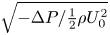 $\sqrt {-\Delta P/\frac {1}{2}\rho U_0^2}$ from experiments. (b) The transverse velocity fluctuations
  $v_{rms}/U_c$, from experiments and DNS of Stanley et al. (2002). (c) The streamwise velocity fluctuations,
  $u_{rms}/U_c$, from the same experiments and DNS.
We can use the classical approach to estimate the orders of magnitude of each term in (2.3); see Appendix B. The relative magnitude of the first term/second term scales like  $\sim 1/x$. Thus the first term in (2.3) is negligible in the far field. From experimental data, in the far field we know that
  $V^2<0.04\,\overline {v'^2}$ (see Heskestad (Reference Heskestad1965) – henceforth HK65; Ramaprian & Chandrasekhara (Reference Ramaprian and Chandrasekhara1985) – henceforth RC85), so
  $V^2$ is also negligible. Thus integrating (2.3) across the jet at any
  $x$ yields
 \begin{equation} -\!\Delta P(x,y) = P_\infty-P(x,y) \approx \gamma_{\Delta p}\,\overline{v'^2}(x,y) , \end{equation}
where  $\overline {v'^2}(y=\pm \infty )=0$, and
  $\gamma _{\Delta p}$ is a constant of order
  $1$ – the corrections due to the neglected terms (the first term and
  $V^2$ in (2.3)) are absorbed into this constant.
The streamwise momentum equation is also modified from the classical approximation – the pressure field is now assumed variable, so the streamwise gradients  $\partial P/\partial x$ and
  $\partial \overline {u'^2}/\partial x$ are not negligible. Hence, we retain these two gradients in (2.2), and together with (2.6) they reflect the improvement in the boundary layer approximation in our theory. Hussain & Clark (Reference Hussain and Clark1977) (henceforth HC77) proposed an approximation similar to (2.6), but they did not propose modifications to the classical approximation to the streamwise momentum equation.
2.1. Non-zero pressure deficit
As  $\overline {v'^2}>0$, it follows from (2.6) that
 \begin{equation} -\!\Delta P(x,y) >0 . \end{equation}
Thus a pressure deficit  $\Delta P<0$ must exist – i.e. lower pressure inside the jet with respect to the ambient pressure is an unavoidable condition in jets.
Not many measurements of the pressure field have been made in TPJs; however, the few cases where it was measured all reveal unambiguous pressure deficit inside the jet. Figure 3(a) displays  $\sqrt {-\Delta P/\frac {1}{2}\rho U_0^2}$ versus
  $\eta (=y/b)$ from Miller & Comings (Reference Miller and Comings1957) (henceforth MC57), and HC77. (Incidentally, pressure deficits have been reported in turbulent axisymmetric jet experiments by Sami, Carmody & Rouse (Reference Sami, Carmody and Rouse1967), Sunyach & Mathieu (Reference Sunyach and Mathieu1969) and Maestrello & McDaid (Reference Maestrello and McDaid1971), and in a co-flowing turbulent jet by Bradbury Reference Bradbury1965).
Measurements of  $u_{rms}$ and
  $v_{rms}$ from HK65 and Gutmark & Wygnanski (Reference Gutmark and Wygnanski1976) (henceforth GW76) are shown in figures 3(b) and 3(c) (because of symmetry in the distributions, we have reflected the data across the jet centreline to yield two overlapping datasets in each case). Also shown for comparison are DNS results (solid line) from Stanley, Sarkar & Mellado (Reference Stanley, Sarkar and Mellado2002) at Reynolds number 4000.
The measurements of  $\sqrt {-\Delta P}$,
  $u_{rms}$ and
  $v_{rms}$ in figure 3 show that the profiles from different experiments and DNS are comparable. From these datasets, we obtain
  $\gamma _{\Delta p}\approx 1.4\mbox{--}1.6$, which is consistent with our theoretical estimate of
  $O(1)$.
Generally, numerical simulations (DNS, Reynolds-averaged Navier–Stokes and large-eddy simulations) have been carried out at much lower Reynolds numbers and shorter jet lengths than in most experiments. These considerations clearly limit the applicability of numerical simulations to our study, except for order of magnitude estimates, such as  $\gamma _{\Delta p}$ above.
2.2. Streamwise momentum flux
Most measurements show the streamwise momentum flux to be decreasing in  $x$ (see figure 4), contradicting the classical claim of momentum flux invariance.

Figure 4. The momentum fluxes from experiments (filled circles): (a)  $J_T$, and (b)
  $J_U$. Numbers in the abscissa identify the experiments listed in table 1. In (b), the horizontal line is
  $J_U=0.9$ as a reference (computed from HC77 data).
Table 1. The momentum fluxes and other characteristics from TPJ experiments. (Unless otherwise stated in the final column, experiments were carried out in air jets emerging from a wall into air at room temperature, with confining walls, and measurements were made using hot wires.) Abbreviations: Bicknell (Reference Bicknell1937) (BIC37), Cafiero & Vassilicos (Reference Cafiero and Vassilicos2019) (CV19), Forthmann (Reference Forthmann1936) (FO36), Goldschmidt & Eskimazi (Reference Goldschmidt and Eskimazi1966) (GE66), Goldschmidt & Young (Reference Goldschmidt and Young1975) (GY75), Gutmark & Wygnanski (Reference Gutmark and Wygnanski1976) (GW76), Hussain & Clark (Reference Hussain and Clark1977) (HC77), Householder & Goldschmidt (Reference Householder and Goldschmidt1969) (HG69), Jenkins & Goldschmidt (Reference Jenkins and Goldschmidt1973) (JG73), Knystautas (Reference Knystautas1964) (KY64); Kotsovinos (Reference Kotsovinos1975, Reference Kotsovinos1978) and Kotsovinos & List (Reference Kotsovinos and List1977) (collectively, KL77); Matsubara, Alfredsson & Segalini (Reference Matsubara, Alfredsson and Segalini2020) (MA20), Nakaguhi (Reference Nakaguhi1961) (NA61), Ramaprian & Chandrasekhara (Reference Ramaprian and Chandrasekhara1985) (RC85), Van der Hegge Zijnen (Reference Van der Hegge Zijnen1958) (VA58). Most of the momentum fluxes in columns 3 and 4 are from KL77 and RC85. LDA is Laser Doppler Anemometry.

 $^{{{\dagger}} }$The CV19 quoted value,
  $J_U=0.94$, has been adjusted appropriately to account for the turbulent contribution; see the text just before the end of § 2.
HC77 were the first to address the problem of momentum flux directly, and took special care in measuring the fluxes accurately. They found that the pressure inside the jet is less than the ambient, and substantial and commensurate increases, up to 56 %, in the momentum fluxes in  $x$.
$x$.
In surprising contrast, Kotsovinos (Reference Kotsovinos1975, Reference Kotsovinos1978) and Kotsovinos & List (Reference Kotsovinos and List1977) (henceforth collectively KL77) measured a momentum flux reduction, and constructed a theory based on this observation. Schneider (Reference Schneider1985) predicted theoretically a momentum flux reduction of approximately 20 % for a jet. (In fact, his theory predicts that momentum flux vanishes as  $x\rightarrow \infty$; see his figure 3.)
These highly contradictory results form one of the major challenges that we resolve in this paper. Later, we show how LSA provides a decisive answer to this puzzle.
Table 1 summarizes the streamwise momentum fluxes ( $J_T$,
  $J_U$ and
  $J_u$) measurements in TPJs since 1934. (Most of the momentum fluxes (JT and JU) were taken from KL77 and RC85.) Abbreviations for different datasets, for identification purposes, are also listed in table 1.
Measurements of  $J_T$ are rare – we have found just seven (four of these are from HC77), which are shown as filled circles plotted versus the experiment number (see table 1) in figure 4(a). Measurements of
  $J_U$ are more plentiful (see figure 4b). The HC77 measurements show that both
  $J_T$ and
  $J_u$ increase in
  $x$ (see figure 6):
  $J_T$ increases by up to 56 % of
  $J_{T0}$ (figure 6b), and
  $J_u$ increases up to approximately 10 % of
  $J_{T0}$ (figure 6c). Thus
  $J_U (=J_T- J_u)$ increases by up to 46 % of
  $J_{T0}$ (figure 6d).
We can establish a fundamental relationship between the momentum flux and the pressure deficit from the improved streamwise momentum balance equation. Let  $x_s$ be some location where the self-preserving region starts – data suggest that, typically,
  $x_s\approx 20$. Integrating (2.2) across the jet at any
  $x\geqslant x_s$, we obtain the streamwise gradient of the total momentum flux (noting that
  $\partial \Delta P/\partial x = \partial P/\partial x)$:
 \begin{equation} \frac{\partial}{\partial x} \left({J_T +\frac{1}{J_{T0}} \int_{-\infty}^\infty \Delta P \,{\rm d}\eta }\right) ={-}\frac{1}{J_{T0}}\,[(UV + \overline{u'v'})]_{-\infty}^\infty =0 . \end{equation}
The right-hand side of (2.8) is zero because  $-UV=0$ and
  $\overline {u'v'}=0$ at
  $\eta =\pm \infty$.
Then, using (2.6) in (2.8) and integrating from  $x= x_s$ to some arbitrary
  $x> x_s$, we obtain
 $$\begin{gather} J_T(x) + \frac{1}{J_{T0}} \int_{-\infty}^\infty \Delta P \,{\rm d}\eta = \left({J_T + \frac{1}{J_{T0}} {\int_{-\infty}^\infty \Delta P \,{\rm d}\eta }}\right)_{x=x_s} \end{gather}$$
 $$\begin{gather}{\rm or}\quad J_T(x) = J_T^{xs} + \frac{\gamma_{\Delta p}}{J_{T0}} \int_{-\infty}^\infty \overline{v'^2}(x,\eta) \,{\rm d}\eta > 1,\quad x\gtrsim x_s, \end{gather}$$
where  $J_T^{xs}$ is the right-hand side of (2.9) (evaluated at
  $x_s$).
There is no theory for the pressure field in the near and intermediate regions  $x< x_s$, so it is not possible to obtain
  $J_T^{xs}$ theoretically. However, data on the mean pressure field (see figure 5, from HC77), show a rapid increase in
  $-\Delta P$ in these regions, indicating significant generation of turbulence, i.e. of
  $\overline {v'^2}$; so we must have
  $J_T^{xs}>1$, hence
  $J_T>1$, before entering the self-preserving region.

Figure 5. The centreline mean pressure deficit distribution  $-\Delta P_c/\frac {1}{2}\rho U_0^2$ versus
  $x/H$ (from HC77, inlet fully turbulent cases).
From data,  $J_u$ is approximately 10 % of
  $J_T$ in the far field (figure 6c); hence we estimate that
 \begin{equation} J_U(x) \approx 0.9J_T(x) > 0.9 \quad {\rm for} \ x\gtrsim x_s, \end{equation}
which must also be satisfied – approximately equivalent to  $J_T> 1$. Though less accurate than (2.10), (2.11) is often more useful because
  $J_U$ is easier to measure, hence there are many more reported measurements of
  $J_U$ than of
  $J_T$ (figure 4). The horizontal line
  $J_U=0.9$ in figure 4(b) is shown as reference. (The threshold of
  $0.9$ is a generic value; in any given experiment, an appropriate threshold must be used.)

Figure 6. (a) The mass flux  $Q_m(x)$. (b–d) The momentum fluxes of, respectively,
  $J_T$,
  $J_u$,
  $J_U$ from HC77 (symbols), and theory fitted to the data (solid lines), versus
  $x$. The legend in (c) is common to all the panels. Here, and in subsequent figures, the vertical dashed line indicates the approximate start of the self-preserving region (inferred qualitatively from congruence of mean velocity profiles).
Condition  $J_T(x)>1$ is a key prediction of our theory – it is a necessary condition that any jet data and any jet theory must satisfy.
The seven data points in figure 4(a) show that  $J_T>1$ – four of these are from HC77, and five correspond to the experiments where we also observe
  $J_U>0.9$ (table 1). The variation in
  $J_U$ between different experiments is large, between
  $0.63$ and
  $1.42$, and only five of the twenty-one experiments show an increase such that
  $J_U>0.9$. (Apart from the four HC77 data points, only one other measurement satisfies this condition!) Other experiments show
  $J_U< 0.9$, even in some experiments that measured pressure deficit within the jet (experiments 1 and 2 in table 1), violating the momentum flux conditions (2.10) and (2.11). We conclude that most measurements of TPJs in the past are not fully reliable.
(Note that the CV19 (see table 1) value  $J_U=0.94$ comes after non-dimensionalizing by the inlet momentum flux of only the mean flow – not including the contribution from the mean momentum flux due to the turbulence – whereas we non-dimensionalize by the total inlet momentum flux
  $J_{T0}$. Assuming that
  $\overline {u_0'^2}/U_0^2\approx 10\,\%$, then from (2.11), CV19 overpredicts
  $J_U$ by approximately 10 %; hence
  $J_U\approx 0.85$ in table 1. Indeed, in figure 8(a) in CV19, after an immediate drop,
  $J_U$ does not show a clear increase as a function of
  $x$.)
$x$.)
We mentioned earlier that the experimental result  $\partial P/\partial y\not =0$ has been, surprisingly, almost totally ignored – no previous theory of turbulent jets has used it. But this result is highly significant because it establishes the improved balance equations from which the existence of a pressure deficit and hence the non-invariance of the momentum flux follow. We claim that a viable jet theory should predict the pressure deficit inside the jet, and hence the non-invariance of the momentum flux.
3. New jet scaling laws via LSA
Lie symmetry analysis has a long history and has been applied in many fields. A summary of LSA of functions and differential equations (DEs), its history and methods, has been elucidated in Appendix A.
The LSA of DEs involves a transformation of the DEs, containing the same physical information as the original DEs. The LSA simply transforms the system to a form where the solution structure is more apparent. The important point is that LSA by itself does not solve the physical problem represented by the system of DEs. Hence additional modelling assumptions – such as closures, separation of variables, scaling laws – must be presented to solve the physical problem fully. For example, LSA of the balance equations in mechanics does not remove the closure problem but simply shifts it to the symmetries. If the physical system truly possesses the symmetries posed by the LSA, then the system of DEs should collapse to simpler forms, typically reduced order of the DEs, revealing deeper insight into the physics. An example is Noether's theorem, which states that every continuous symmetry of the action of a physical system with conservative forces has a corresponding conservation law (mass conservation, energy conservation, momentum balance, etc.), and vice versa.
Note that LSA works well only for closed systems of equations. When dealing with unclosed equations, one can always generate an infinite Lie-algebra of invariant transformations. One can generate numerous statistical equivalences and thus also numerous statistical scaling laws, among which are not only physical ones, but also a myriad of non-physical ones that cannot be realized by the governing Navier–Stokes equations, hence remaining unreflected in the data. A discussion on these issues is contained in Frewer, Khuujadze & Foysi (Reference Frewer, Khuujadze and Foysi2014), Frewer (Reference Frewer2022), Brethouwer (Reference Brethouwer2023), Frewer & Khujadze (Reference Frewer and Khujadze2023a,Reference Frewer and Khujadzeb,Reference Frewer and Khujadzec) and Oberlack et al. (Reference Oberlack, Hoyas, Kraheberger, Alcántara-Ávila and Laux2022, Reference Oberlack, Hoyas, Laux and Klingenberg2023). Oberlack and co-authors claim that symmetry analysis of the underlaying statistical symmetries of the Navier–Stokes equations overcomes the closure problem. But Frewer and Brethouwer and co-authors claim that the Lie group symmetry method as used by Oberlack et al. cannot bypass the closure problem of turbulence: ‘the fact that the invariant solution method of Lie-group symmetries should not be used for unclosed systems in the same way as for closed systems still holds true’ (Frewer & Khujadze Reference Frewer and Khujadze2023c).
3.1. The LSA of the jet balance equations
We assume that all jet flow statistics are smooth (continuous and differentiable), which allows us to apply LSA to the whole domain. We apply LSA to both the governing partial differential equations (PDEs) and the boundary conditions. We have two independent variables  $({\boldsymbol {x}})=(x,y)$, and several dependent variables,
  $({\boldsymbol {u}})=(U,V,P,\Delta P, \overline {u'^2}, \overline {v'^2}, R,k,G,P_r,\epsilon )$, where
  $R=-\overline {u'v'}$,
  $k=(\overline {u'^2}+ \overline {v'^2}+ \overline {w'^2})/2$,
  $G=\overline {v'(u'^2+v'^2+w'^2+p')}$ and
  $P_r= -\overline {u'v'}({\partial U}/{\partial y})$.
The TPJ balance equations in the new boundary layer approximation are
 $$\begin{gather} \frac{\partial U}{\partial x} + \frac{\partial V}{\partial y} = 0 , \end{gather}$$
 $$\begin{gather}\frac{\partial (U^2+\overline{u'^2}+P)}{\partial x} + \frac{\partial (UV+\overline{u'v'})}{\partial y} = 0 , \end{gather}$$
 $$\begin{gather}\Delta P(x,y) ={-} \gamma_{\Delta p}\,\overline{v'^2}(x,y) , \end{gather}$$
 $$\begin{gather}R(x,y) = C^2\,U_c(x)\,b\,\frac{{\rm d}b}{{\rm d}\kern 0.06em x}\,\frac{{\rm d}U}{{\rm d}y}, \end{gather}$$
 $$\begin{gather}U\,\frac{\partial k}{\partial x} + V\,\frac{\partial k}{\partial y} ={-}\frac{\partial G}{\partial y} + P_r - \epsilon . \end{gather}$$
An eddy-viscosity model (discussed further in § 4.7) has been invoked in (3.4), namely  $R=\nu _t({\textrm {d}U}/{\textrm {d}y})$, where the eddy viscosity is
  $\nu _t = C^2U_c b({\textrm {d}b}/{\textrm {d}\kern0.7pt x})$. Note that
  $\nu _t$ includes a dependence on the transverse length scale, the jet half-width
  $b(x)$, which has already been defined implicitly as
  $U(x,b)=U_c(x)/2$.
In (3.1)–(3.4), there are six variables,  $U(x,y)$,
  $V(x,y)$,
  $P(x,y)$,
  $\overline {u'^2}(x,y)$,
  $\overline {v'^2}(x,y)$ and
  $R=\overline {u'v'}(x,y)$, but only four equations. To obtain exact LSA solutions, we would need to close the system of equations by posing models for two of the variables.
However, an alternative approach is to obtain scaling laws from the unclosed equations, with the understanding that these are not true symmetry transformations, but only equivalence relations that map one unclosed system of equations to another, yielding families of solutions dependent on Lie symmetry parameters (see below). These families will contain physical as well as unphysical solutions. Later, we determine which of these are true physical solutions by applying models and other physical assumptions (such as separation of variables and self-preservation) to variables, and matching the obtained scaling laws to data. We pursue the alternative approach here.
The TKE equation (3.5) introduces new unknowns but is unclosed, hence it cannot close the system of equations. But the TKE equation stands on its own, and scaling laws for  $k$,
$k$,  $G$,
$G$,  $P_r$ and
  $\epsilon$ can still be derived. We include it here for future reference.
The boundary conditions are unchanged:
 \begin{equation} \left.\begin{gathered} \hbox{at } y=0, \quad U=U_c(x), \quad V=0, \quad \frac{{\rm d}U}{{\rm d}y}=0, \quad -\overline{u'v'}=0,\\ \hbox{at } y={\pm} \infty, \quad U=0, \quad P=P_\infty, \quad -\overline{u'v'}=0. \end{gathered}\right\}\end{equation}
 Our theory requires a model for  $J_U (x)$, for which we pose
 \begin{equation} J_U(x) = J_U^{xs} + C_U (x^q-x_s^q), \quad x\geqslant x_s , \end{equation}
where  $q$ changes slowly in
  $x$. Here,
  $C_U$ is a constant that depends on initial and boundary conditions. In the far field,
  $q(x)\to q_0$ as
  $x\to \infty$, where
  $-1\ll q_0 \ll 1$. Thus
  $J_U$ increases without limit, or asymptotes to a constant value equal to
  $J_U^{xs}$ or
  $J_U^{xs}-C_Ux_s^{q_0}$.
Furthermore, the relationship  $J_T=J_U+J_u$ implies that all three momentum fluxes must scale in the same way
  $\sim x^{q}$, with coefficients such that
  $C_T=C_U+C_u$.
Let  $\varPsi$ designate the system of jet PDEs and boundary conditions and the models for
  $J_U$ equations: (3.1)–(3.7). A body of literature suggests that the most appropriate symmetries that can be applied to turbulent jets are translation in the streamwise coordinate
  $x$, and dilatations in all coordinates (She, Chen & Hussain Reference She, Chen and Hussain2017; Chen, Hussain & She Reference Chen, Hussain and She2018; Layek & Sunita Reference Layek and Sunita2018b). The general infinitesimal forms of the global symmetry group of transformations (A29) and (A30), consisting of one translation
  $(-a_0)$ in
  $x$, and dilatations in all variables (
 $a_1,a_2,\ldots$), are
 \begin{equation} \left.\begin{gathered} \xi_x={-}a_0+a_1x,\quad \xi_y=a_2y,\quad \eta_u=a_3U,\quad \eta_v=a_vV,\quad \eta_p =a_p P,\\ \eta_{\Delta p}=a_p\,\Delta P, \quad \eta_R=a_R R,\quad \eta_{\overline{u'^2}}=a_{\overline{u'^2}}\,\overline{u'^2},\quad \eta_{\overline{v'^2}}=a_{\overline{v'^2}}\,\overline{v'^2}, \\ \eta_k=a_k k, \quad \eta_G=a_G G, \quad \eta_{P_r}=a_{P_r}P_r, \quad \eta_\epsilon=a_\epsilon\epsilon, \quad b(x)=a_bb, \end{gathered}\right\} \end{equation}
where  $a_0\in \mathbb {R}$ is a translation, and
  $a_1,a_2,a_3,a_v,\ldots \in \mathbb {R}$ are dilatation group parameters. Note that because
  $P-\Delta P=P_\infty$, which is a constant, the scalings of
  $\Delta P$ and
  $P$ with
  $x$ are the same.
The Lie operator is  $X = \xi _x({\partial }/{\partial x}) + \xi _y({\partial }/{\partial y}) + \eta _u({\partial }/{\partial u}) + \eta _v({\partial }/{\partial v}) + \eta _p({\partial }/{\partial p}) +$
  $\eta _R({\partial }/{\partial R}) + \cdots$. However, for the structurally simple modelling ansatz (3.8), it is not necessary to use the full LSA machinery, and
  $X(\varPsi )=0$ is not needed because the solutions can be read from the equations. Here,
  $\varPsi$ is invariant under the one translation (
 $-a_0$) and two dilation (
 $a_1,a_2$) symmetry groups of transformations
  $G_{a_0}$,
  $G_{a_1}$ and
  $G_{a_2}$, which we combine as
  $G_{a_0}\circ G_{a_1s}\circ G_{a_2}$ to yield the finite multi-parametric group representation
 \begin{equation} \left.\begin{gathered}
\tilde{x}={\rm e}^{a_1}(x-a_0/a_1)+a_0/a_1, \quad
\tilde{y}={\rm e}^{a_2}y,\quad \tilde{U}={\rm e}^{a_3}U,\quad
\tilde{V}={\rm e}^{a_V}V,\quad \tilde{R}={\rm e}^{a_R}R, \\
\widetilde{\Delta P}={\rm e}^{a_P}\,\Delta P, \quad
\tilde{P}={\rm e}^{a_P}P, \quad \widetilde{\overline{u'^2}}=
{\rm e}^{a_{\overline{u'^2}}}\,\overline{u'^2},\quad
\widetilde{\overline{v'^2}}={\rm e}^{a_{\overline{v'^2}}}\,\overline{v'^2},\\
\tilde{k}={\rm e}^{a_k}k,\quad \tilde{G}={\rm e}^{a_G}G, \quad
\tilde{\epsilon}={\rm e}^{a_\epsilon}\epsilon, \quad
\widetilde{P_r}={\rm e}^{a_{P_r}}P_r, \quad
\tilde{b}={\rm e}^{a_b}b.
\end{gathered}\right\}\end{equation}
\begin{equation} \left.\begin{gathered}
\tilde{x}={\rm e}^{a_1}(x-a_0/a_1)+a_0/a_1, \quad
\tilde{y}={\rm e}^{a_2}y,\quad \tilde{U}={\rm e}^{a_3}U,\quad
\tilde{V}={\rm e}^{a_V}V,\quad \tilde{R}={\rm e}^{a_R}R, \\
\widetilde{\Delta P}={\rm e}^{a_P}\,\Delta P, \quad
\tilde{P}={\rm e}^{a_P}P, \quad \widetilde{\overline{u'^2}}=
{\rm e}^{a_{\overline{u'^2}}}\,\overline{u'^2},\quad
\widetilde{\overline{v'^2}}={\rm e}^{a_{\overline{v'^2}}}\,\overline{v'^2},\\
\tilde{k}={\rm e}^{a_k}k,\quad \tilde{G}={\rm e}^{a_G}G, \quad
\tilde{\epsilon}={\rm e}^{a_\epsilon}\epsilon, \quad
\widetilde{P_r}={\rm e}^{a_{P_r}}P_r, \quad
\tilde{b}={\rm e}^{a_b}b.
\end{gathered}\right\}\end{equation} For convenience, we define the variables  $x_0$ and
  $n_* = a_*/a_1$ (where the ‘
 $*$’ stands for any variable) as follows:
 $$\begin{gather} x_0 = \frac{a_0}{a_1}, \end{gather}$$
 $$\begin{gather}n_a = \frac{a_2}{a_1}, \end{gather}$$
 $$\begin{gather}n_q = \frac{q}{a_1}, \end{gather}$$
where  $a_1\not = 0$. (Note that in the far field,
  $x_0$ is not relevant.)
It will simplify the following steps if we anticipate the scaling for the length scale  $b(x)\sim x^{n_a}$ in (3.35); thus
  $n_b=a_b/a_1=n_a$.
Thus inserting (3.9) into (3.1)–(3.5), and demanding it to be an equivalence transformation such that (3.1)–(3.5) remain invariant, leads to the following expressions for the group parameters:
 $$\begin{gather} n_{v^2} = n_{u^2}, \end{gather}$$
 $$\begin{gather}n_U-1 = n_V - n_a, \end{gather}$$
 $$\begin{gather}2n_U -1 = n_{u^2}-1 = n_{v^2}-1 = n_U+n_V-n_a = n_R -n_a, \end{gather}$$
 $$\begin{gather}n_U+n_k -1 = n_V+n_k -n_a = n_G-n_a = n_{P_r} = n_\epsilon. \end{gather}$$
 The transformations must be consistent with the models for  $J_U$, and the transformations for the composite variables
  $R:=\nu _t\, \partial U/\partial y$ and
  $P_r:= R\, \partial U/\partial y$ must be consistent with their respective constituent variables. These give the further restrictions
 $$\begin{gather} 2n_U + n_b = n_q, \end{gather}$$
 $$\begin{gather}n_{u^2}+ n_b = n_q, \end{gather}$$
 $$\begin{gather}n_R = 2n_U +2n_b-1-n_a, \end{gather}$$
 $$\begin{gather}n_{P_r} = n_R+n_U-n_a. \end{gather}$$
These restrictions yield the following expressions for the transformation group parameters (with  $n_b=n_a$):
 $$\begin{gather} n_U= \frac{a_3}{a_1} = \frac{-n_a+n_q}{2} , \end{gather}$$
 $$\begin{gather}n_V= \frac{a_v}{a_1} = n_U +n_a-1 ={-}1 +\frac{n_a+n_q}{2}, \end{gather}$$
 $$\begin{gather}n_R= \frac{a_R}{a_1} ={-}1 +n_q , \end{gather}$$
 $$\begin{gather}n_{u^2} =\frac{a_{\overline{u'^2}}}{a_1} ={-}n_a+n_q, \end{gather}$$
 $$\begin{gather}n_{v^2} = \frac{a_{\overline{v'^2}}}{a_1} ={-}n_a+n_q, \end{gather}$$
 $$\begin{gather}n_p = \frac{a_p}{a_1} = n_{v^2} ={-}n_a+n_q, \end{gather}$$
 $$\begin{gather}n_{\Delta p} = \frac{a_{\Delta p}}{a_1} = n_{v^2} ={-}n_a+n_q . \end{gather}$$
And from the TKE equation we obtain
 $$\begin{gather} n_{P_r} = \frac{a_{P_r}}{a_1} ={-}1 - \frac{3n_a-3n_q}{2} , \end{gather}$$
 $$\begin{gather}n_\epsilon = \frac{a_{\epsilon}}{a_1} = n_{P_r} ={-}1 - \frac{3n_a-3n_q}{2} , \end{gather}$$
 $$\begin{gather}n_G = \frac{a_{G}}{a_1} ={-}1 - \frac{n_a-3n_q}{2} , \end{gather}$$
 $$\begin{gather}n_k = \frac{a_k}{a_1} ={-}n_a + n_q . \end{gather}$$
Inserting all of these into (3.8), we obtain
 \begin{equation} \left.\begin{gathered} \xi_x=a_1\left({x-x_0}\right), \quad \eta_y=a_1\left({n_a}\right)y, \quad \eta_b=a_1\left({n_a}\right)b, \quad \eta_U={-}a_1\left(\frac{n_a-n_q}{2}\right)U, \\ \eta_V={-}a_1\left({1-\frac{n_a+n_q}{2}}\right)V, \quad \eta_{\Delta p}={-}a_1\left({n_a-n_q}\right)\Delta P, \\ \eta_{p}={-}a_1\left({n_a-n_q}\right)P, \quad \eta_{\overline{u'^2}}={-}a_1\left({n_a-n_q}\right)\overline{u'^2}, \quad \eta_{\overline{v'^2}}={-}a_1\left({n_a-n_q}\right)\overline{v'^2},\\ \eta_R={-}a_1\left({1-n_q}\right)R, \quad \eta_k={-}a_1\left({n_a-n_q}\right)k, \quad \eta_G={-}a_1\left({1+\frac{n_a-3n_q}{2}}\right)G, \\ \eta_{P_r}={-}a_1\left({1+\frac{3n_a-3n_q}{2}}\right)P_r, \quad \eta_\epsilon={-}a_1\left({1+\frac{3n_a-3n_q}{2}}\right)\epsilon. \end{gathered}\right\}\end{equation}
The associated characteristic equations are
 \begin{align} & \frac{{\rm d}\kern0.7pt x}{x-x_0} = \frac{{\rm d} y}{n_ay} = \frac{{\rm d}b}{n_ab} = \frac{{\rm d}U}{-\left({\dfrac{n_a-n_q}{2}}\right)U} = \frac{{\rm d}V}{-\left({1-\dfrac{n_a+n_q}{2}}\right)V} \nonumber\\ &= \frac{{\rm d}\Delta P}{-\left({n_a-n_q}\right)\Delta P} = \frac{{\rm d}P}{-\left({n_a-n_q}\right)P} = \frac{{\rm d}\overline{u'^2}}{-\left({n_a-n_q}\right)\overline{u'^2}} = \frac{{\rm d}\overline{v'^2}}{-\left({n_a-n_q}\right)\overline{v'^2}} \nonumber\\ &= \frac{{\rm d}R}{-\left({1-n_q}\right)R}= \frac{{\rm d}k}{-\left({n_a-n_q}\right)k} = \frac{{\rm d}G}{-\left({1+ \dfrac{n_a-3n_q}{2}}\right)G} = \frac{{\rm d}P_r}{-\left({1+ \dfrac{3n_a-3n_q}{2}}\right)P_r} \nonumber\\ &= \frac{{\rm d}\epsilon}{-\left({1+ \dfrac{3n_a-3n_q}{2}}\right)\epsilon}. \end{align}
 Clearly, for non-zero translation we have  $a_0\not = 0$, and for non-zero dilatations we have
  $a_1\not = 0$ and
  $a_2\not = 0$.
In the ensuing, the superscript  $*$ refers to unscaled variables. The first two ratios in (3.33) give
 \begin{equation} \hat{\eta} = \frac{y^*}{H^*}\left({\frac{x^*-x^*_0}{H^*}}\right)^{{-}n_a}, \quad\hbox{or}\quad \frac{y^*}{H^*} = \hat{\eta} x^{n_a} \quad {\rm where} \ x=\frac{x^*-x^*_0}{H^*} . \end{equation}
Here,  $H^*$ is a characteristic length scale such as the slit width, and
  $x$ is the streamwise similarity variable. The jet half-width
  $b$ scales as
 \begin{equation} b = \frac{b^*}{H^*} = b_u\left({\frac{x^*-x^*_0}{H^*}}\right)^{n_a} = b_u x^{n_a}, \end{equation}
where  $b_u$ is a constant (the spread rate coefficient) that depends on initial and boundary conditions.
We define a second, more commonly used, transverse similarity variable
 \begin{equation} \eta = \frac{y^*}{b^*} \left({= \frac{\hat{\eta}}{b_u} }\right). \end{equation}
 The spreading rate  $\alpha$, the rate of change of the jet half-width, is
 \begin{equation} \alpha = \frac{{\rm d}b}{{\rm d}\kern0.7pt x} = n_ab_ux^{n_a-1}, \end{equation}
where  $\alpha$ depends on the initial and boundary conditions. (With
  $n_a=1$, we recover the classical constant jet spreading rate
  $\alpha =b_u$.)
The boundary conditions are also form-invariant:
 \begin{equation} \left.\begin{gathered} \hbox{at } \eta=0, \quad U=U_c(x), \quad V=0, \quad \frac{{\rm d}U}{{\rm d}\eta}=0, \quad -\overline{u'v'}=0,\\ \hbox{at } \eta ={\pm} \infty, \quad U=0, \quad P=P_\infty, \quad -\overline{u'v'}=0. \end{gathered}\right\}\end{equation}
 By solving the characteristic equations (3.33), scaling laws for other quantities are obtained as functions of  $x$ and
  $\eta$.
3.2. The self-preserving scaling laws
Invoking separation of variables, self-preserving solutions of all flow variables in the far field take the form  $F(x,\eta )=F_c (x)\,f(\eta )$, where
  $F_c (x)$ denotes the centreline streamwise distribution of the jet variable, and
  $f(\eta )$ is the associated profile.
Solving (3.33) under these assumptions, we obtain (recollect that  $P$ is the kinematic pressure
  $P/\rho$)
 $$\begin{gather} \frac{U}{U_0} \approx A x^{-({n_a-n_q})/{2}}\,f_U(\eta), \end{gather}$$
 $$\begin{gather}\frac{V}{U_0} \approx A x^{{-}1+{(n_a+n_q)}/{2}}\,f_V(\eta), \end{gather}$$
 $$\begin{gather}\frac{-\overline{u^{\prime}v^{\prime}}}{U^2_0} \approx A^2 x^{{-}1+n_q}\,f_R(\eta), \end{gather}$$
 $$\begin{gather}\frac{\overline{{u^{\prime}}^2}}{U^2_0} \approx A^2 x^{{-}n_a+n_q}\,f^2_u(\eta) , \end{gather}$$
 $$\begin{gather}\frac{\overline{{v^{\prime}}^2}}{U^2_0} \approx A^2 x^{{-}n_a+n_q}\,f^2_v(\eta) , \end{gather}$$
 $$\begin{gather}\frac{P}{U^2_0} \approx A^2 x^{{-}n_a+n_q}\,f_{p}(\eta), \end{gather}$$
 $$\begin{gather}\frac{\Delta P}{U^2_0} \approx A^2 x^{{-}n_a+n_q}\,f_{\Delta p}(\eta), \end{gather}$$
 $$\begin{gather}\frac{k}{U^2_0} \approx A^2 x^{{-}n_a+n_q}\,f_{k}(\eta), \end{gather}$$
 $$\begin{gather}\frac{G}{U^3_0} \approx A^3 x^{{-}1-{(n_a-3n_q)}/{2}}\,f_{G}(\eta), \end{gather}$$
 $$\begin{gather}\frac{P_r}{U^3_0} \approx A^3 x^{{-}1-{(3n_a-3n_q)}/{2}}\,f_{P_r}(\eta), \end{gather}$$
 $$\begin{gather}\frac{\epsilon}{U^3_0} \approx A^3 x^{{-}1-{(3n_a-3n_q)}/{2}}\,f_{\epsilon}(\eta) . \end{gather}$$
We will assume that  $A=1$.
It was long assumed that the jet behaviour in the self-preserving region is independent of initial conditions. However, around the 1990s, studies suggested that such a state is unlikely to exist; rather, there exists a multiplicity of self-preserving states each one of which is determined by its initial conditions, whose influence never disappears (Wygnanski, Champagne & Marasli Reference Wygnanski, Champagne and Marasli1986; George Reference George1989, Reference George2012; George & Gibson Reference George and Gibson1992; George & Davidson Reference George and Davidson2004; Hickey, Hussain & Wu Reference Hickey, Hussain and Wu2013). The scaling laws above are not universal because  $n_a$ and
  $n_q$ depend on other flow parameters (such as the Reynolds number). But the scaling laws are consistent with George's hypothesis of a multiplicity of self-preserving states, each state characterized by different Lie group parameters, namely the translation
  $x_0$, the jet spread exponent
  $n_a$, and the momentum flux exponent
  $n_q$.
3.3. Asymptotic form of  $J_T(x)$

We obtain  $J_T(x)$ from (2.10) using (3.43):
 \begin{align} J_T(x) &= J_T^{xs} + \left[{\frac{1}{J_{T0}}\int_{-\infty}^\infty \rho \gamma_{\Delta p}\,\overline{v'^2}(x,\eta)\,b \,{\rm d} \eta}\right]_{x_s}^x \quad {\rm for}\ {x\geqslant x_s} \end{align}
 \begin{align} &= J_T^{xs} + \left({\frac{\rho \gamma_{\Delta p} A^2U_0^2b_U}{J_{T0}}\int_{-\infty}^\infty f_v^2(\eta) \,{\rm d}\eta}\right) \left[{x^{n_q}}\right]_{x_s}^x\quad {\rm for}\ {x\geqslant x_s}. \end{align}
The integral inside the parentheses converges under the mild condition that the profile approaches zero faster than  $f_v(\eta ) < 1/|\eta |^{0.5}$ as
  $|\eta |\to \infty$ – data show that
  $f_v$ converges to zero much faster than this. Furthermore, if the profile is self-preserving, then the integral is a constant. Thus, absorbing all constants together in
  $C_T$, we obtain
 \begin{equation} J_T(x) = J_T^{xs} + C_T (x^{n_q}-x_s^{n_q}),\quad {x\geqslant x_s}. \end{equation}
Thus in the far field,  $J_T(x)\sim x^{n_q}$, which scale like
  $J_U(x)$ and
  $J_u(x)$ as expected. Here,
  $n_q$ is small and in the range
  $-1\ll n_q\ll 1$ as
  $x\to \infty$. Negative
  $n_q$ in the far field does not violate
  $J_T>1$ (which reflects the increase in the total momentum flux); it means that
  $J_T\to J_T^{xs}-C_Tx_s^{n_q}>1$ (a constant) as
  $x\to \infty$. If
  $n_q=0$ in the far field, then
  $J_U\to J_T^{xs}>1$ (a different constant) as
  $x\to \infty$. Positive
  $n_q$ in the far field would imply that
  $J_T\to \infty$ as
  $x\to \infty$. Thus far downstream,
  $J_T$ (hence also
  $J_U$ and
  $J_u$) could asymptote very slowly to a constant value, or increase without bound.
4. Results
In this section, the  $x$ variation of flow variables is plotted against the scaled streamwise coordinate
  $x$ for the theoretical curves, and against
  $x=x^*/H$ for the data (assuming that these are equivalent for
  $x\gg x_0$ in the far field).
We obtain  $x_0$, the translation of the coordinate system, from data; in the HC77 datasets,
  $x_0\approx 5$. Measurements further show that the self-preserving part of a jet in most TPJs starts from approximately
  $x_s\approx 20$.
4.1. The mass and momentum fluxes
HC77 paid particular attention to accurate measurements of mass and momentum fluxes. They measured  $Q_m$,
  $J_T$ and
  $J_u$ for different inlet conditions (figure 6). Cases N-50 and N-125 have laminar top-hat flow exit profiles, and C-50 and C-125 emerge from a long channel producing fully developed turbulent flow at the inlet. The -50 cases were at
  $Re=32\,550$, and the -125 cases were at
  $Re=81\,400$.
Our task is to evaluate  $n_a$ and
  $n_q$ from data. In view of the limited data and experimental uncertainties, we fit via inspection by eye.
We obtain  $n_Q$ from fits to
  $Q_m(x)$. In the far field,
  $x\geqslant 20$, using (3.39) in (1.1), we have
 $$\begin{gather} Q_m(x) = \frac{1}{Q_0}\int_\infty^\infty \rho b\,U(x,\eta) \,{\rm d}\eta = x^{(n_a+n_q)/2}\left({\frac{\rho U_0 b_u}{Q_0}\int_{-\infty}^{\infty}f_U(\eta) \,{\rm d}\eta }\right),\quad x\geqslant 20 , \end{gather}$$
 $$\begin{gather}\Rightarrow\quad Q_m(x) \approx C_Q x^{n_Q},\quad {\rm where}\ n_Q=(n_a+n_q)/2, \quad x \geqslant 20, \end{gather}$$
with  $C_Q=Q_m(x_s)/x_s^{n_Q}$. The integral converges provided that
  $|\,f_U(\eta )|< 1/|\eta |$ as
  $|\eta |\to \infty$; data show that
  $f_U(\eta )$ approaches zero faster than this.
The following functions give good agreement with  $Q_m$ in HC77 in the range
  $x\geqslant 20$ (figure 6a):
 $$\begin{gather} Q_m(x) \approx 0.629x^{0.55} \quad \hbox{for N-50}, \end{gather}$$
 $$\begin{gather}Q_m(x) \approx 0.604x^{0.54} \quad \hbox{for N-125}, \end{gather}$$
 $$\begin{gather}Q_m(x) \approx 0.604x^{0.54} \quad \hbox{for C-50}, \end{gather}$$
 $$\begin{gather}Q_m(x) \approx 0.536x^{0.54} \quad \hbox{for C-125}, \end{gather}$$
where  $n_Q =(n_a+n_q)/2 \approx 0.55$ for the N-50 jet, and
  $0.54$ for the other jets. The
  $n_Q$ values are approximately 10 % greater than the classical value
  $0.5$, but they differ little between the four different jets.
For the momentum fluxes, we obtain
 $$\begin{gather} J_T(x) = J_T^{xs} + C_T (x^{n_{q}}-x_s^{n_{q}}), \end{gather}$$
 $$\begin{gather}J_U(x) = J_U^{xs} + C_U (x^{n_q}-x_s^{n_q}), \end{gather}$$
 $$\begin{gather}J_u(x) = J_u^{xs} + C_u(x^{n_{q}}-x_s^{n_{q}}). \end{gather}$$
The constants  $C_T$,
  $C_U$ and
  $C_u$ depend on initial and boundary conditions.
The following functions give good agreement with  $J_T$ in HC77 in the range
  $x \geqslant 20$ (figure 6b):
 $$\begin{gather} J_T \approx 1.500 + 0.349(x^{0.12}-x_s^{0.12}) \quad \hbox{for N-50}, \end{gather}$$
 $$\begin{gather}J_T \approx 1.425 + 0.306(x^{0.11}-x_s^{0.11}) \quad \hbox{for N-125}, \end{gather}$$
 $$\begin{gather}J_T \approx 1.332 + 0.261(x^{0.08}-x_s^{0.08}) \quad \hbox{for C-50}, \end{gather}$$
 $$\begin{gather}J_T \approx 1.185 + 0.159(x^{0.05}-x_s^{0.05}) \quad \hbox{for C-125}. \end{gather}$$
The following functions give good agreement with  $J_u(x)$ in the range
  $x\geqslant 20$ (figure 6c):
 $$\begin{gather} J_u \approx 0.107 + 0.004(x^{0.27}-x_s^{0.27}) \quad \hbox{for N-50}, \end{gather}$$
 $$\begin{gather}J_u \approx 0.108 + 0.026(x^{0.20}-x_s^{0.20}) \quad \hbox{for N-125}, \end{gather}$$
 $$\begin{gather}J_u \approx 0.112 + 0.040(x^{{-}0.10}-x_s^{{-}0.10}) \quad \hbox{for C-50}, \end{gather}$$
 $$\begin{gather}J_u \approx 0.115 + 0.026(x^{0.15}-x_s^{0.15}) \quad \hbox{for C-125}. \end{gather}$$
 HC77 did not measure  $J_U$, but it is obtained from
  $J_U=J_T-J_u$. In the range
  $x\geqslant 20$, we obtain (figure 6d)
 $$\begin{gather} J_U \approx 1.330 + 0.162(x^{0.31}-x_s^{0.31}) \quad \hbox{for N-50}, \end{gather}$$
 $$\begin{gather}J_U \approx 1.270 + 0.147(x^{0.26}-x_s^{0.26}) \quad \hbox{for N-125}, \end{gather}$$
 $$\begin{gather}J_U \approx 1.197 + 0.125(x^{0.24}-x_s^{0.24}) \quad \hbox{for C-50}, \end{gather}$$
 $$\begin{gather}J_U \approx 1.056 + 0.067(x^{0.20}-x_s^{0.20}) \quad \hbox{for C-125}. \end{gather}$$
The results (4.3)–(4.21) yield estimates for  $n_a$ and
  $n_q$ listed in table 2. The estimates for
  $n_q$ in the three fluxes from RC85 (below) are reasonably consistent, but those in the HC77 jets are not fully consistent. For example, from the N-50 experiment, we obtain
  $n_q\approx 0.12 (J_T)$,
  $0.27 (J_u)$ and
  $0.31 (J_U)$. The differences in the values of
  $n_q$ (
 $0.12, 0.27, 0.31$) between the three fluxes is most likely due to the jet length
  $40H$ being too short for the jet to have reached true self-preserving states, hence only approximating our theory, which assumes self-preservation.
Table 2. Estimated quantities.

The differences in  $n_q$ between different jets are not surprising since we expect different asymptotic states depending on initial and boundary conditions (see references to George et al. mentioned above). However, it is notable that all jets, except HC77-C50 (
 $J_u$), show positive
  $n_q$ – indicating that
  $J_T$ would increase without bound far downstream. (In the HC77-C50 jet we also have
  $n_{v^2}\approx 1.26$ (table 3), which differs notably from the other HC77 jets and the RC85 jet – suggesting that the measurements in the HC77-C50 jet may not be reliable.) Of the three fluxes,
  $J_U$ is the easiest to measure accurately, hence the scaling laws obtained from
  $J_U$ are preferred in the ensuing.
Table 3. The negative exponents  $-n_*$ in the scaling law of flow variable
  $x$ distributions (
 ${\sim }x^{n_*}$) calculated from
  $n_a$ and
  $n_q$ in table 2 and (3.39)–(3.49). The mass flux exponent
  $Q_m\sim x^{n_Q}$ has positive exponent. Note that
  $n_k = n_p=n_{\Delta P} = n_{v^2}= n_{u^2}$ and
  $n_{P_r} = n_\epsilon$.

The increases in  $J_T$ at the end of the jet exit at
  $x=40$, reported by HC77, are 56 % (N-50), 48 % (N-125), 35 % (C-50) and 20 % (C-125). In a recent study, MA20 stated that
  $J_U$ was ‘constant’ in their measurements; however, a close examination of their own data (figure 3a in MA20) reveals that
  $J_U$ in fact increased by approximately 12 % for a configuration comparable to C-125. In the HC77 case C-125 (table 1),
  $J_T$ increases by approximately 18 % and
  $J_u$ by approximately 12 %; the 6 % difference is the increase in
  $J_U$ – in reasonable agreement with MA20.
From figure 6, we observe that in terms of magnitude,  $J_U\approx 0.9 J_T$ and
  $J_u\approx 0.1 J_T$. We have already taken this as a working rule in (2.11).
To address the question of whether  $J_T$ peaks and then decays, or continues to increase in the far field, requires an in-depth study; at the current time, there are insufficient data to draw conclusions on this, but it will be addressed in the future when more data are available in longer jets. We will nevertheless proceed with the current parameter values, but with the caution that our conclusions are limited to short-length TPJs.
4.2. Nonlinear growth of $b(x)$

Most TPJ data show the jet half-width growth to be linear in  $x$, i.e.
  $b(x)\sim x^1$. Our theory predicts that
  $b(x)$ has a nonlinear dependence on
  $b(x)\sim x^{n_a}$. There could be many reasons for this; one reason is that different exponents close to
  $1$ cannot be distinguished over the short distances in most experiments. A jet length in the far field section of approximately a decade is necessary to accurately determine
  $n_a$ from
  $b(x)$, i.e. approximately
  $20\lesssim x\leqslant 200$ – no previous study has satisfied this requirement, and it is a major challenge for both lab experiments and numerical simulation.
We also note that although theoretically  $n_a$ could be greater than 1, table 2 shows that in reality all the jets display
  $n_a<1$.
4.3. The $x$ variations

Figure 7 plots the scaling law exponents of the  $x$ variation of the mean variables versus
  $n_a$ from our theory for the cases with
  $n_q=0.31$: the mean velocities
  $U\sim x^{n_U}$,
  $V\sim x ^{n_V}$ and the variance
  $\overline {u'^2} \sim x^{n_{u^2}}$ (figure 7a), and the turbulent diffusion of TKE
  $G\sim x^{n_G}$, and the dissipation
  $\epsilon \sim x ^{n_\epsilon }$ (figure 7b). All other variables possess one of these scaling laws; see (3.39)–(3.49). The mass flux is
  $Q_m\sim x ^{n_Q}$, the streamwise mean momentum flux is
  $J_U\sim x^{n_q}$, and the jet half-width is
  $b\sim x^{n_a}$. The Reynolds shear stress scales like
  $R\sim x^{n_R}$, where
  $n_R=-1+n_q$ is independent of
  $n_a$ hence it is not shown.

Figure 7. Scaling law exponents versus  $n_a$, with
  $n_q=0.31$, for (a) the mean velocities
  $n_U$ and
  $n_V$, and turbulence variance
  $n_{u^2}$, and (b) turbulent diffusion
  $n_G$ and dissipation
  $n_\epsilon$.
As an example (from HC77 case N-50), if  $n_a=0.79$ and
  $n_q=0.31$, then
  $U\sim x^{-0.24}$,
  $V\sim x^{-0.45}$,
  $\overline {u'^2} \approx x^{-0.48}$,
  $\overline {v'^2} \approx x^{-0.48}$,
  $P \sim x^{-0.48}$,
  $\Delta P \sim x^{-0.48}$,
 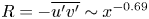 $R=-\overline {u'v'}\sim x^{-0.69}$,
  $G\sim x^{-0.93}$,
 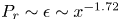 $P_r \sim \epsilon \sim x^{-1.72}$, and
  $Q_m\sim x^{0.55}$,
  $b\sim x^{0.79}$,
  $J_U\sim x^{0.31}$. The corresponding classical scaling laws are (
 $n_a=1, n_q=0$), respectively:
  $U\sim x^{-0.5}$,
  $V\sim x^{-0.5}$,
  $\overline {u'^2}\sim x ^{-1}$,
  $\overline {v'^2}\sim x ^{-1}$,
  $R\sim x^{-1}$,
  $P=P_\infty$,
  $\Delta P=0$,
  $G\sim x^{-1.5}$,
  $P_r\sim \epsilon \sim x^{-2.5}$, and
  $Q_m\sim x^{0.5}$,
  $J_U=1$,
  $b \sim x^1$.
Our theory predicts that the TPJ angle at any  $x$,
$x$,  $\theta (x)$, given by (3.37) as
  $\tan (\theta )=\alpha =b_u n_a x^{n_a-1}$, is not constant. Thus if
  $n_a< 1$, then
  $\tan (\theta )\sim x^{n_a-1}\to 0$ as
  $x\to \infty$, i.e. the jet angle at any
  $x$ in the far field is smaller than classically, approaching zero at infinity; however, as
  $1-n_a\ll 1$, this is a very slow flattening out of the jet. Thus the incompressible jet spreads more slowly in
  $x$ than the classical linear growth, and the streamwise mean velocity
  $U\sim x^{-(n_a-n_q)/2}$ decays more slowly than classically.
Finally, the momentum flux exponent  $n_q$ is small and positive in RC85 and HC77 jets (table 2), indicating a slow rate of increase in the momentum fluxes with
  $x$.
$x$.
4.4. Estimating parameters from $x$ variations

We have quantified  $n_a$ and
  $n_q$ in the HC77 jets from the
  $x$ distribution of mass and momentum fluxes. We would like to quantify them in other jets; however, these fluxes are rarely measured over a significant range of
  $x$ – the only additional measurement of
  $J_T(x)$ that we have found where
  $J_T>1$ is satisfied is in RC85. We will also consider HK65 and GW76 as examples of quantifying jet parameters from other flow metrics.
RC85 recorded  $J_T$ and
  $U_c\sim x^{-(n_a-n_q)/2}$. The latter is plotted as
 \begin{equation} \left({\frac{U_0}{U_c}}\right)^2 \approx K1\,x^{n_a-n_q}, \quad x\geqslant 20, \end{equation}
where  $K1$ is a constant that depends on initial and boundary conditions. Figure 8 shows the RC85 data and our theory for
  $J_T(x)$ and
  $({{U_0}/{U_c}})^2$:
 $$\begin{gather} J_T(x) \approx 1.455 + 0.41(x^{0.10}-x_s^{0.10}), \quad x\geqslant 20, \end{gather}$$
 $$\begin{gather}\left({\frac{U_0}{U_c}}\right)^2 \approx 0.48 x^{0.85}, \quad x\geqslant 20, \quad{\rm with}\ n_a-n_q=0.75. \end{gather}$$
With  $n_q\approx 0.1$ and
  $n_a-n_q\approx 0.85$, we obtain
  $n_a\approx 0.95$. (Separately, from plots of
  $b(x)$, we found that
  $b_u\approx 0.12$ and
  $K1\approx 0.48$.)

Figure 8. Plots of (a)  $J_T$ versus
  $x$ for different
  $n_q$, and (b)
  $(U_0/U_c)^2$ versus
  $x$ for different
  $n_a-n_q$. Data from RC85 (symbols) and theory (lines). The vertical line is defined in figure 6.
For HK65 and GW76, we fit to  $(U_0/U_c)^2$ and
  $b(x)$ (they did not measure the mass or momentum fluxes) – with the caution that the exponent in
  $b(x)$ could be subject to significant uncertainty because of the inherent jet flow geometry constraints. Fortunately, the far field ranges (
 $20\leqslant x\leqslant 100$ and
  $20< x\leqslant 150$) were longer than in HC77 – approximately factors of 5 and 7.5, respectively – which reduces the uncertainty. Reasonable fits to the HK65 data (figure 9) are
 $$\begin{gather} \left({\frac{U_0}{U_c}}\right)^2 \approx 0.30 x^{0.96}, \quad x\geqslant 20, \quad{\rm with}\ n_a-n_q=0.91, \end{gather}$$
 $$\begin{gather}b(x) \approx 0.17 x^{0.90}, \quad x\geqslant 20, \end{gather}$$
hence  $n_q= -0.06$,
  $n_a=0.90$,
  $K1=0.30$ and
  $b_u\approx 0.17$. And for the GW76 data, reasonable fits (figure 10) are
 $$\begin{gather} \left({\frac{U_0}{U_c}}\right)^2 \approx 0.22 x^{0.95}, \quad x\geqslant 20, \quad{\rm with}\ n_a-n_q=0.93 \end{gather}$$
 $$\begin{gather}b(x) \approx 0.16 x^{0.89}, \quad x\geqslant 20, \end{gather}$$
hence  $n_q= -0.06$,
  $n_a=0.89$,
  $K1\approx 0.22$ and
  $b_u\approx 0.16$.

Figure 9. Plots of (a)  $(U_0/U_c)^2$ versus
  $x$ for different
  $n_a-n_q$, and (b)
  $b(x)$ versus
  $x$ for different
  $n_a$. Data from HK65 (symbols) and theory (lines). The vertical line is defined in figure 6.

Figure 10. Plots of (a)  $(U_0/U_c)^2$ versus
  $x$ for different
  $n_a-n_q$, and (b)
  $b(x)$ versus
  $x$ for different
  $n_a$. Data from GW76 (symbols) and theory (lines). The vertical line is defined in figure 6.
The estimated quantities obtained from all jet cases considered are listed in table 2.
We note that a nonlinear spread rate of the jet width has also been obtained by Cafiero & Vassilicos (Reference Cafiero and Vassilicos2019) and Layek & Sunita (Reference Layek and Sunita2018b) based on the idea that jets are in a state of non-equilibrium turbulence. But they start from the classical momentum balance equations, i.e. following the classical boundary layer approximation – which we have challenged here.
4.5. The TKE variables
The  $x$ variations of
  $k$,
$k$,  $G$,
$G$,  $P_r$ and
  $\epsilon$ are difficult to measure and thus rarely obtained. From reliable datasets where
  $J_T>1$, we have not found any such measurements. A few measurements exist for
  $\epsilon$ in jets where
  $J_T<1$ (which is not possible), hence such results are not reliable. Validation of these scaling laws will be addressed when data become available.
4.6. Estimating $x$ variations of other flow variables

Based on the estimated values of  $n_a$ and
  $n_q$ in the different jets, the (negative) exponents of the scaling laws for the other flow variables are obtained from (3.39)–(3.49), and are listed in table 3. The Reynolds number
  $Re$, the momentum flux condition (
 $J_T >1$) and the mass flux exponent
  $n_Q=(n_a+n_q)/2$ are also shown in table 3.
HK65 and GW76 do not satisfy the momentum flux condition  $J_T<1$, thus are less reliable than the other datasets.
4.7. The profiles
RC85 and HC77 satisfy the admissibility condition  $J_T>1$. We therefore base the following discussions on these five sets of measurements. The variations in
  $n_a$ and
  $n_q$ between these five different jets is significant, which is consistent with our assumption of the existence of a multiplicity of states.
To complete the analysis, we need to validate the predictions for the profiles of flow variables from our theory – a stringent test of the theory.
To determine the profiles, we put the new scaling laws in (3.39)–(3.49) into the balance equations and obtain relationships between the different profiles. For  $f_V$, we obtain
 \begin{equation} \frac{f_V}{b_u n_a} = \eta f_U - \left({\frac{n_a+n_q}{2n_a}}\right) F_U, \end{equation}
where  $F_U (\eta )= \int _0^\eta f_U(s)\,\textrm {d}s$. The Reynolds shear stress profile, to leading order, is given by
 \begin{equation} \frac{1}{b_un_a}\,f_R =\left({\frac{n_a+n_q}{2n_a}}\right)f_UF_U. \end{equation}
Equation (3.3) gives
 \begin{equation} f_{\Delta p} \approx{-}\gamma_{\Delta p} f^2_v. \end{equation}
The boundary conditions are
 \begin{equation} \left.\begin{gathered} \hbox{at } \eta=0, \quad f_U=1, \quad f_V=0, \quad \frac{{\rm d}f_U}{{\rm d}\eta}=0, \quad f_R=0, \\ \hbox{at } \eta={\pm} \infty, \quad f_U=0, \quad f_{\Delta p}=0, \quad f_R=0. \end{gathered}\right\}\end{equation}
 Thus if  $f_U$ is known, then
  $f_V$ can be calculated from (4.29), and
  $f_R$ can be calculated from (4.30). If
  $f_v$ is also known or modelled, then
  $f_{\Delta p}$ can be calculated from (4.31) – datasets for
  $f_v$ and
  $f_{\Delta p}$ exist, as we have seen in figure 3.
We cannot calculate  $f_k$,
  $f_G$ and
  $f_\epsilon$ without additional assumptions; however, they are related through the TKE equation
 \begin{equation} \left({\frac{f_V}{b_un_a} -\eta f_U }\right)\frac{\partial f_k}{\partial \eta} - \left({{\frac{n_a+n_q}{n_a}}}\right)f_Uf_k ={-} \frac{1}{b_un_a}\,\frac{\partial f_G}{\partial \eta} + \frac{f_{P_r} - f_\epsilon}{n_a} . \end{equation}
If  $f_U$ and
  $f_V$, and the coefficients of the terms on the left-hand side, are known, then only
  $f_G$,
  $f_{P_r}$ and
  $f_\epsilon$ need further modelling. This is outside of the scope of this paper, but will be addressed in the future.
Solutions for jet transverse profiles in (4.29)–(4.31) are obtained using a closure for the Reynolds shear stress (3.4),  $-\overline {u'v'}=\nu _t \,\textrm {d}U/{\textrm {d} y}$, and we model the eddy viscosity by
 \begin{equation} \nu_t = C^2 U_c b\,\frac{{\rm d}b}{{\rm d}\kern0.7pt x} . \end{equation}
 The velocity scale is the mean centreline velocity  $U_c (x)$, the length scale is the jet half-width
  $b(x)$, and
  $C$ is a constant. The eddy-viscosity model, although a simple model, captures the main physical principles and consequences of our theory, and produces closed-form solutions. Using (4.34) in (4.30) yields
  $f_R (\eta )= -b_u\,F_U''(\eta )$ and
  $F_U (\eta )=1/N \tanh (N\eta )$, where
  $N(x)=({1}/{2C})\sqrt {{(n_a+n_q)}/{n_a}}$. Hence we obtain the solutions
 $$\begin{gather} f_U \approx {\rm sech}^2 (N\eta), \end{gather}$$
 $$\begin{gather}f_V \approx b_u n_a \eta\, {\rm sech}^2 (N\eta) -2C^2 b_u n_a N \tanh(N\eta) , \end{gather}$$
 $$\begin{gather}f_R \approx 2C^2 b_u n_a N\,{\rm sech}^2 (N\eta)\tanh(N\eta), \end{gather}$$
 $$\begin{gather}f_{\varDelta P} \approx{-}\gamma^2_{\Delta p}\,f_{\overline{v'^2}}, \quad{\rm where}\ \gamma_{\Delta p}=O(1). \end{gather}$$
 The eddy-viscosity model does not account for the intermittent entrainment of turbulent flow into the jet across the turbulent–non-turbulent interface, which affects the profiles of turbulent quantities. A leading-order correction is to weight the turbulent profiles with an entrainment intermittency factor  $f_\gamma (\eta )$ across the jet. Figure 11 summarizes the data (symbols) from HK65 and GW76 for
  $f_\gamma$ versus the transverse coordinate
  $\eta$ and the fit (solid line) that we use.

Figure 11. Profiles of the intermittency factor  $f_\gamma$. Experiments (symbols) and fit to data (solid line) – the average of HK65 and GW76.
For comparison with data, RC85 is the only admissible and (nearly) complete dataset that we have found. (HC77 did not present the profiles of the mean transverse velocity or the Reynolds shear stress.) We therefore focus on the RC85 data to compare with our predictions. Here,  $n_a$,
  $n_q$ and
  $b_u$ have already been determined (table 2). For
  $C$, we pose solutions to the profiles in (4.35)–(4.38) and determine the value of
  $C$ of best fit.
Figure 12 shows the RC85 data for  $f_U$,
  $f_V$ and
  $f_R$ (symbols) and our theory (lines) with
  $n_a= 0.95$,
  $n_q= 0.10$ (table 2), with an estimated
  $b_u= 0.12$, for different values of the eddy-viscosity parameter
  $C$. All profiles display the correct form and orders of magnitude against data. The best fit for
  $f_U$ is
  $C\approx 0.7$; the best fit for
  $f_V$ is
  $C\approx 0.8$; and the best fit for
  $f_R$ is
  $C\approx 0.5$. The estimate for
  $C$ is therefore in the range
  $0.50\lesssim C\lesssim 0.8$. The good match of the Reynolds stress profile to data is important because it is a second-order turbulence statistical quantity.

Figure 12. From RC85, profiles of (a)  $f_U$, (b)
  $f_V$, and (c)
  $f_R$, from data (symbols) compared with model predictions for different
  $C$ as indicated (lines), with
  $n_a=0.95$,
  $n_q=0.10$ and
  $b_u=0.12$ (see table 2).
Figure 13 shows the RC85 data for  $v_{rms}$. They did not measure the pressure distribution, but using figure 3(a) as a benchmark, with estimated
  $\sqrt {\gamma _{\Delta p}}\approx 1.18$, we obtain an estimate for
  $\sqrt {-\Delta P}$, also shown in figure 13.

Figure 13. Profile of  $v_{rms}$ from RC85 (filled circles) against
  $\eta$. Also shown is
  $\sqrt {-\Delta P/0.5\rho U_0^2} =1.18 v_{rms}$ (open circles), which compares well with MC57 in figure 3(a).
5. Summary
We propose a new theory for high Reynolds number, incompressible, turbulent plane jets (TPJs) in the far field. The cornerstone of our theory is the realization that the jet is not truly ‘thin’, as implied by the classical boundary layer approximation. As a consequence, some of the streamwise and transverse gradients of flow variables and the momentum fluxes previously ignored are retained in our analysis, yielding improved momentum balance equations (3.2) and (3.3). Hence the pressure deficit, proportional to the variance of the transverse velocity fluctuations, is significant, and the total streamwise momentum flux must increase with  $x$, i.e.
  $J_T (x)>1$ – which is a necessary admissibility condition that any viable experiment, numerical simulation or theory must satisfy.
Furthermore, applying Lie symmetry analysis (LSA) to the refined momentum balance equations produces a new family of scaling laws for flow variables and fluxes whose  $x$ exponents differ from previous predictions by up to approximately 20 %, which is very significant. The LSA with translational and dilatational transformations produces families of scaling laws (3.39)–(3.49) for flow variables as functions of the parameters
  $x_0$ (the coordinate translation),
  $n_a$ (the jet spread exponent),
  $n_q$ (the momentum flux exponents) and the modelling constants
  $b_u$ (the jet spread coefficient; see (3.35)) and
  $C$ (the eddy-viscosity coefficient). Our theory predictions agree with measurements reported in the literature satisfying the admissibility condition (
 $J_T>1$) – see tables 2 and 3, and figures 12 and 13; the profiles of
  $U$,
$U$,  $V$ and
  $-\rho \,\overline {u'v'}$, and the pressure deficit, are well predicted. Although theoretically the jet growth, the half-width
  $b(x)\sim x^{n_a}$, can have
  $n_a>1$, our review of measurements shows that in reality all TPJs with
  $J_T>1$ display sublinear growth with
  $n_a<1$, i.e. the TPJs are narrower than classically, with smaller jet spread angle that approaches zero as
  $x\to \infty$ (the jets flatten out at infinity). In general, our results differ notably from the predictions of classical theory. For example,
  $U$ decays more slowly with
  $x$ than in classical theory (tables 2 and 3).
Finally, the review of past experiments (table 1, figure 4) has revealed that most past experiments are not fully reliable, and those that are (satisfying  $J_T>1$) are typically from short-length jets. Clearly, up-to-date and accurate experiments and simulations (DNS and large-eddy simulations) over long streamwise lengths (for asymptotic conditions) are needed. A special focus must be placed on accurate measurements of the pressure, the mass and momentum fluxes, the transverse velocity fluctuations, and full three-dimensional velocity measurements.
Acknowledgements
The authors thank Dr E. Garcia for reviewing the manuscript and plotting figure 2 using DNS plane jet simulation data of N. Peralta.
Declaration of interests
The authors report no conflict of interest.
Data availability
The data that support the findings of this study are available within the paper.
Appendix A. The LSA of DEs
A.1. History
Lie symmetry analysis has a long history, going back to the pioneering work of Sophius Lie (and Felix Klein) in the late nineteenth century, although LSA did not feature prominently in fluid mechanics until the 1990s; see Cantwell (Reference Cantwell2002) and Arrigo (Reference Arrigo2015). Lie symmetry analysis addresses the invariances of DEs, often describing physical systems, that are analysed and interpreted using groups of transformations (translations, rotations, etc.). Lie showed that all such DEs could be brought into a unified approach in terms of infinitesimals of the transformations. Thus LSA enables one to determine all continuous symmetry groups of transformations (translations, rotations, dilatations, etc.) under which the written forms of both the governing DEs and the associated boundary conditions remain unchanged (i.e. are form-invariant). By combining the symmetry transformations of the DE variables, the LSA method determines all solutions of the governing DEs; see Bluman & Kumei (Reference Bluman and Kumei2013) and Cantwell (Reference Cantwell2002).
Lie's ideas remained largely unrecognized until after the Second World War, when Ovasiannikov (Reference Ovasiannikov1978) and Birkhoff (Reference Birkhoff1960) drew attention to his work, followed by Bareneblatt & Zel'dovich (Reference Bareneblatt and Zel'dovich1972). There followed an ‘awakening’ to Lie's ideas in many other sciences, especially in fluid mechanics and mathematical physics. Bytev (Reference Bytev1972), Andreev & Rodionov (Reference Andreev and Rodionov1988), Andreev et al. (Reference Andreev, Kaptsov, Vladislav and Rodionov1998), Oberlack (Reference Oberlack1999, Reference Oberlack2001, Reference Oberlack2002) and Cantwell (Reference Cantwell2002) were among the first to apply LSA to fluid mechanical systems. She et al. (Reference She, Chen and Hussain2017) and Chen et al. (Reference Chen, Hussain and She2018) used LSA to investigate wall turbulence described by Reynolds-averaged Navier–Stokes equations. Layek & Sunita (Reference Layek and Sunita2017) applied LSA to decaying isotropic turbulence, axisymmetric turbulent wakes (Layek & Sunita Reference Layek and Sunita2018a), TPJs (Layek & Sunita Reference Layek and Sunita2018b) and plane turbulent plumes (Layek & Sunita Reference Layek and Sunita2018c). Oberlack & Rosteck (Reference Oberlack and Rosteck2010) have applied LSA to statistical symmetries of multi-point turbulence equations. (A statistical symmetry is a symmetry of the DE describing a given statistical moment, e.g. the averaged Navier–Stokes equation (first moment), and the Reynolds shear stress equation (second moment), and so on.) See Klingenberg, Oberlack & Pluemacher (Reference Klingenberg, Oberlack and Pluemacher2020) for a review of LSA methods in turbulence.
A.2. Symmetry of functions
Let the vector  $(\boldsymbol x) = (x^1,x^2,\ldots,x^i)$,
  $i=1,\ldots,m$, lie in some continuous open set
  $D$ of the Euclidean manifold
  $\mathbb {R}^m$. We define the transformation
 \begin{equation} T^s(\boldsymbol x): \{ \tilde x^i = F^i(\boldsymbol{x},s),\ i=1,\ldots,m\}, \end{equation}
where the  $F^i$ are functions of
  $({\boldsymbol {x}})$, infinitely differentiable in
  $C^\infty$, and analytic in the group parameter
  $s$. Here,
  $s$ is a scalar that defines a continuous transformation of variables for every value of
  $s$ on the open interval of the real line
  $\mathcal {H}$ that contains it,
  $s\in \mathcal {H}$. The transformation
  $T^s$ is a one-parameter Lie group. That is, there exists an algebraic structure consisting of a continuous open set
  $\mathcal {H}$ and possessing a binary operation (such as translation, rotation, dilation) that operates on elements of the set
  $\mathcal {H}$ and obeys the rules of group theory, namely: (1) closure under the operation; (2) associativity; (3) existence of a unique identity element of
  $\mathcal {H}$ (typically
  $s=0$ or
  $1$), which corresponds to the identity transformation; (4) existence of unique inverses to every element of
  $\mathcal {H}$ (e.g. a rotation can be reversed by an opposite rotation).
At the heart of symmetry analysis is the concept of an invariant function. This is best illustrated by examples of specific groups of translations and invariant functions under such groups of translation.
Let  $({\boldsymbol x})=(x,y)$ (here,
  $i=1,2$). Then the transformation
  $T^s$ is a one-parameter Lie group in two variables, and is of the form
 \begin{equation} T^s : \{ \tilde x = F^1(x,y,s);\ \tilde y = F^2(x,y,s)\}. \end{equation}
 Under a translation group of transformations, ( ${\boldsymbol {x}}$) transforms as
 \begin{equation} T^s_{tran}: \{ \tilde x = x+a_1s,\ \tilde y = y+a_2s,\ \mathcal{H}= (-\infty,\infty) \}, \end{equation}
where  $a_1$ and
  $a_2$ are real numbers. Under a rotational group of transformations,
  $({\boldsymbol {x}})$ transforms as
 \begin{equation} T^s_{rot}: \{ \tilde{\boldsymbol{x}} = R(s)\,\boldsymbol x,\ \mathcal{H}= [-{\rm \pi},{\rm \pi}) \}, \end{equation}
where  $R(s)$ is the orthogonal matrix for rotation through angle
  $s$. Under a dilatation group of transformations,
  $({\boldsymbol {x}})$ transforms as
 \begin{equation} T^s_{dil}: \{ \tilde x
= {\rm e}^s x,\ \tilde y = {\rm e}^{ns} y,\ \mathcal{H}=
(-\infty,\infty) \},
\end{equation}
\begin{equation} T^s_{dil}: \{ \tilde x
= {\rm e}^s x,\ \tilde y = {\rm e}^{ns} y,\ \mathcal{H}=
(-\infty,\infty) \},
\end{equation}
where  $n>0$ is a real number for dilatation (interpreted as stretching when
  $s>0$,or contraction when
  $s<0$).
Now consider the transformation of the function  $\rho (x,y)= y/x^4$ for
  $x>0$ under dilatational with
  $n=4$ in (A5), to obtain
 \begin{equation} \rho({\tilde x},
{\tilde y}) = \frac{\tilde y}{\tilde x^4} =
\frac{{\rm e}^{ns}y}{{\rm e}^{4s}x^4} = \frac{y}{x^4} = \rho(x,y).
\end{equation}
\begin{equation} \rho({\tilde x},
{\tilde y}) = \frac{\tilde y}{\tilde x^4} =
\frac{{\rm e}^{ns}y}{{\rm e}^{4s}x^4} = \frac{y}{x^4} = \rho(x,y).
\end{equation}
The right-hand side is independent of the parameter  $s$ for any
  $s$ in the open interval
  $\mathcal {H}$ (in (A5)), and the function remains unchanged in the new dilated coordinates. The function
  $\rho (x,y)= y/x^4$ is form-invariant under the group transformation (A5) for
  $n=4$ – that is, its written form reads identically in original and transformed variables. However, if we set
  $n=5$, then we would obtain
 \begin{equation} \tilde{\rho}
({\tilde{x}}, {\tilde{y}}) = {\rm e}^s\,\frac{y}{x^4}, \quad{\rm
or}\quad \frac{\tilde{\rho}}{{\rm e}^s} = \frac{y}{x^4} =
\rho(x,y) .
\end{equation}
\begin{equation} \tilde{\rho}
({\tilde{x}}, {\tilde{y}}) = {\rm e}^s\,\frac{y}{x^4}, \quad{\rm
or}\quad \frac{\tilde{\rho}}{{\rm e}^s} = \frac{y}{x^4} =
\rho(x,y) .
\end{equation} Thus a given solution curve is not invariant under the group. Nevertheless, the family of curves (as a whole) is invariant under the group – by running through all values of  $s$, the solution curves cover the same solution space.
The parametric representation of smooth functions on a continuous open interval of  $s$ ensures that the mapping is differentiable and invertible (i.e. is a diffeomorphism), and that the mapping functions can be expanded in Taylor series about any value of
  $s$.
$s$.
We can extend the group transformation to include its first derivatives using the notation (Cantwell Reference Cantwell2002)
 \begin{equation} \frac{{\rm d} \tilde{y}}{{\rm d}\tilde{x}} = G_{\{1\}}(x,y,y_x; s). \end{equation}
 For the linear translation (A3), we have  $\textrm {d}\tilde {y}/\textrm {d}\kern0.7pt\tilde {x}={\textrm {d} y}/{\textrm {d}\kern0.7pt x}$, and for the dilatation transformation (A5) (with
  $n=1$) we also have
  $\textrm {d}\tilde {y}/\textrm {d}\kern0.7pt\tilde {x}={\textrm {d} y}/{\textrm {d}\kern0.7pt x}$. This can be extended to any order. The notation for the second-order derivative is
 \begin{equation} \frac{{\rm d}^2 \tilde{y}}{{\rm d}\tilde{x}^2} = G_{\{2\}}(x,y,y_x,y_{xx}; s). \end{equation}
The transformations (A3) or (A5), together with the derivatives (A8), form a group called the once extended group of transformations. Including the second-order derivative (A9) forms a group called the twice extended group of transformations, and so on.
Extended groups are important in solving DEs by replacing occurrences of derivatives by the right-hand sides of (A8), (A9), etc.
These transformations can be generalized to any number of independent and dependent variables. We define the one-parameter Lie group
 \begin{equation} T^s: \{ \tilde{x}^i = f^i(\boldsymbol x,s),\ j=1,\ldots,m\}, \end{equation}
where  $f^i (\boldsymbol x,s)$,
  $i=1,\ldots,m$, are differentiable functions in
  $C^\infty$ and analytic in the group parameter
  $s$. This property allows us to expand functions in Taylor series in the parameter
  $s$. A function
  $\rho (\boldsymbol x;s)$ is invariant under (A10) if and only if
 \begin{equation} \rho(\tilde{\boldsymbol{x}}) = \rho(f^i(\boldsymbol x,s)) =\rho(\boldsymbol x), \end{equation}
i.e. the function is form-invariant in both the original and transformed coordinates, and is independent of  $s$.
$s$.
Equation (A11) is a global transformation, but is not very useful because of the often nonlinear dependence of the  $f^i$ on the group parameter
  $s$. Lie's great contribution was to show that (A11) is equivalent to an infinitesimal invariance condition, also equivalent to a set of linear ordinary DEs, for any system of DEs – far simpler to solve than (A11).
A.3. Infinitesimal invariance condition
The symmetry condition (A11) can also be stated as the condition that the total differential of  $\rho$ on a curve of constant
  $\rho$ (its value being determined by initial conditions) is zero, i.e.
  $\textrm {d}\rho =0$. Such curves are called characteristic curves, and the set of all characteristic curves forms an ‘invariant’ surface.
Because the Lie group transformations are analytic in  $s$, we can expand
  $\rho (\tilde {\boldsymbol {x}})=\rho (f^i ({\boldsymbol {x}},s))$ as a Taylor expansion in
  $s$ about the identity element
  $s=0$:
 \begin{equation} \rho(\tilde {\boldsymbol{x}}) = \rho({\boldsymbol{x}}) + s\left({\frac{\partial \rho}{\partial s}}\right)_{s=0} + \frac{s^2}{2}\left({\frac{\partial^2 \rho}{\partial s^2}}\right)_{s=0} + \cdots. \end{equation}
Using the chain rule and Einstein's summation convention, we obtain
 \begin{equation} \left({\frac{\partial \rho}{\partial s}}\right)_{s=0} = \frac{\partial \rho}{\partial f^i} \left({\frac{\partial f^i}{\partial s}}\right)_{s=0} = \xi^i\,\frac{\partial \rho}{\partial f^i}, \end{equation}
where
 \begin{equation} \xi^i=\left({\frac{\partial f^i}{\partial s}}\right)_{s=0} \end{equation}
are called infinitesimals. Put this into (A12) to obtain the Lie series representation of  $\rho$:
 \begin{equation} \rho(\tilde{\boldsymbol{x}}) = \rho({\boldsymbol{x}}) + s\left(\xi^i\,{\frac{\partial \rho}{\partial x^i}}\right) + \frac{s^2}{2!}\,\xi^i\,\frac{\partial}{\partial x^i}\left(\xi^k\,{\frac{\partial \rho}{\partial x^k}}\right) + \cdots.\end{equation}
This is true for all  $s$, so the invariance condition
  $\rho (\tilde {\boldsymbol {x}})=\rho ({\boldsymbol {x}})$ is satisfied if and only if each term is zero; hence the infinitesimal condition (replacing
  $f^i$ with
  $x^i$)
 \begin{equation} \xi^i \left({\frac{\partial \rho}{\partial x^i}}\right) = 0 \end{equation}
must be satisfied. Equation (A16) is a linear first-order PDE and is far more useful than the global condition (A11) – indeed, in Lie theory, one is almost always working with linear invariance conditions.
Equation (A16) defines the equations of the characteristic curves:
 \begin{equation} \frac{{{\rm d}\kern0.7pt x}^i}{{\rm d}s} = \xi^i,\quad i=1,\ldots,m. \end{equation}
The  $m-1$ associated characteristic equations are first-order ordinary DEs written compactly as
 \begin{equation} \frac{{{\rm d}\kern0.7pt x}^1}{\xi^1} = \frac{{{\rm d}\kern0.7pt x}^2}{\xi^2} = \cdots= \frac{{{\rm d}\kern0.7pt x}^m}{\xi^m}={\rm d}s. \end{equation}
A characteristic curve is invariant under the group since it lies on the invariant surfaces. The  $m-1$ integrals of (A18),
 \begin{equation} \rho^i = \int \frac{{{\rm d}\kern0.7pt x}^i}{\xi^i} = {\rm const}^i,\quad i=1,2,\ldots, m-1, \end{equation}
which depend on initial conditions (at  $s=s_0$), are the invariants of the group
  $T^s$.
We define the group operator as
 \begin{equation} X = \xi^i\,\frac{\partial}{\partial x^i}, \end{equation}
and  $X\rho = \xi ^i (\partial \rho /\partial x^i)$ is called the Lie derivative of
  $\rho$. Substituting for
  $X$ and
  $X\rho$ in (A12), and with some rearrangement, we obtain
 \begin{align} \rho(\tilde{\boldsymbol{x}}) &= \rho({\boldsymbol{x}})+ sX\rho + \frac{1}{2!}\,sX(sX\rho) \nonumber\\ &= \left({ 1+sX+\frac{(sX)^2}{2!} + \cdots}\right)\rho({\boldsymbol x}), \end{align}
which can be written compactly as  $\rho (\tilde {\boldsymbol {x}})=e^{sX}\,\rho (\boldsymbol {x})$.
Finally, we note that there may be isolated points that are invariant under the group. These are the critical points of (A17) and correspond to the roots of the equation
 \begin{equation} \xi^i({\boldsymbol{x}}) = 0. \end{equation}
A.4. The LSA of DEs
The LSA of DEs has been used in many fields, including physics and fluid mechanics; see Cantwell (Reference Cantwell2002), Oberlack (Reference Oberlack2002) and Arrigo (Reference Arrigo2015). Subsection A.1 presents a summary of its historical development, and the principles and methods of LSA applied to functions – finding the symmetry invariants of a function is the core of the LSA theory. It delineates the analytical framework for LSA of systems of PDEs, because in LSA, PDEs are viewed as locally analytic functions in an extended space, called jet space, whose coordinates are all the independent and dependent variables, and the various partial derivatives of the dependent variables with respect to the independent variables.
Consider a system of  $M$ PDEs characterizing a physical system:
 \begin{equation} \varPsi^l({\boldsymbol{x,u,u}}_1,{\boldsymbol{u}}_2,\ldots,{\boldsymbol{u}}_p) = 0, \quad l=1,2,\ldots,M . \end{equation}
The jet space in this notation has  $({\boldsymbol {x}})=(x^1,x^2,\ldots,x^m)$ as the
  $m$ independent variables and
  $({\boldsymbol {u}})=(u^1,u^2,\ldots,u^n)$ as the dependent variables, and
  $\boldsymbol {u}_p$ denotes all possible
  $p$th-order partial derivatives of
  $({\boldsymbol {u}})$ with respect to
  $({\boldsymbol {x}})$.
A continuous one-parameter group of transformations is denoted by
 \begin{equation} G_s: {\boldsymbol {\tilde{x}}}=\boldsymbol{\phi}({\boldsymbol{x}}, {\boldsymbol{u}}, s), {\tilde{\boldsymbol{u}}}=\boldsymbol{\chi}({\boldsymbol{x}}, {\boldsymbol{u}}, s), \end{equation}
where  $(\boldsymbol {\phi }, \boldsymbol {\chi }): D\times \mathcal {H}\to D$,
  $D \subseteq \mathbb {R}^{m+n}$, and
  $s\in \mathcal {H} \subset \mathbb {R}$, is called the symmetry group of transformations of (A24) if it remains form-invariant under
  $G_s$ – that is, the written form of (A23) remains identical when expressed in the transformed coordinates. This statement is true if and only if
 \begin{equation} \varPsi^l (\tilde{\boldsymbol{x}}, \tilde{\boldsymbol{u}}, \tilde{\boldsymbol{u}}_1,\ldots, \tilde{\boldsymbol{u}}_p) \iff \varPsi^l(\boldsymbol{x}, \boldsymbol{u}, \boldsymbol{u}_1,\ldots,\boldsymbol{u}_p), \quad l=1,2,\ldots,M . \end{equation}
The transformations  $G_s$ satisfy the group properties (Cantwell Reference Cantwell2002). The transformation functions
  $(\phi,\chi )$ (referred to as
  $f^j$ in equation (A10)) are analytic in the group parameter
  $s$.
$s$.
The LSA algorithm can be applied to virtually any system of PDEs, and constitutes probably the most important and widely applicable method for finding analytical solutions of nonlinear problems.
To give an example, we consider Burgers’ equation,
 \begin{equation} \frac{\partial u}{\partial t} + u\,\frac{\partial u}{\partial x} - \nu\,\frac{\partial^2 u}{\partial x^2}=0, \end{equation}
which can be re-stated as a function (with  $M=1$) in jet space as
 \begin{equation} \varPsi\left[{t,x,u,\frac{\partial u}{\partial t},\frac{\partial u}{\partial x}, \frac{\partial^2 u}{\partial x^2},\frac{\partial^2 u}{\partial x\,\partial t},\frac{\partial^2 u}{\partial t^2}}\right] = 0 \end{equation}
whose coordinates are  $({\boldsymbol {x}})=(t,x)$,
  $(\boldsymbol {u})=u$,
  $(\boldsymbol {u}_{1})=(\partial u/\partial t,\partial u/\partial x)$ and
  $(\boldsymbol {u}_{2})=({\partial ^2 u}/{\partial x^2},$
  ${\partial ^2 u}/{\partial x\,\partial t},{\partial ^2 u}/{\partial t^2})$, where we take all the possible first- and second-order derivatives of
  $u$ with respect to
  $x$ and
  $t$. The derivative of
  $\varPsi$ with respect to
  $\partial u/\partial t$ is 1, with respect to
  $u$ is
  $\partial u/\partial x$, with respect to
  $\partial u/\partial x$ is
  $u$, and with respect to
  $\partial ^2 u/ \partial x^2$ is
  $-\nu$ – all other derivatives are zero.
The infinitesimal transformations corresponding to  $G_s$ are obtained by Taylor series expansion about the identity element
  $s=0$ (recall that
  $s$ is the group parameter):
 \begin{equation} G_s:\left\{\begin{array}{@{}ll@{}} \tilde{x}^i= x^i+s\xi^i, & i=1,2,\ldots,m,\\[2pt] \tilde{u}^j= u^j+s\eta^j, & j=1,2,\ldots,n, \end{array} \right. \end{equation}
where the infinitesimals of  $G_s$,
  $\xi ^i$ and
  $\eta ^j$, are smooth functions given by
 $$\begin{gather} \xi^i = \left.\frac{{\rm d}\phi^i}{{\rm d}s}\right|_{s=0}, \quad i=1,2,\ldots,m, \end{gather}$$
 $$\begin{gather}\eta^j = \left.\frac{{\rm d}\chi^j}{{\rm d}s}\right|_{s=0}, \quad j=1,2,\ldots,n. \end{gather}$$
The group operator is (summation convention applying)
 \begin{equation} X = \xi^i\,\frac{\partial }{\partial x^i} + \eta^j\,\frac{\partial }{\partial u^j}, \end{equation}
and  $X\varPsi$ is the Lie derivative of
  $\varPsi$. Any system of PDEs that is analytic in
  $s$ can be expanded as a Lie series – a Taylor series in
  $s$ with ‘derivative’
  $X$.
$X$.
The group operator can be prolonged (or extended) to the  $p$th extended group operator
  $X_{\{p\}}$ by including in the expansion on the right-hand side of (A31) derivatives with respect to
  $\boldsymbol {u}_1, \boldsymbol {u}_2,\ldots, \boldsymbol {u}_p$ up to order
  $p$. (Cantwell (Reference Cantwell2002) gives a rigorous derivation of
  $X_{\{p\}}$ for the general case of any number of independent and dependent variables, and to any order of prolongation.) Typically,
  $p= 0$,
  $1$ or
  $2$ is sufficient for most real-world applications (where
  $X=X_{\{0\}}$).
For the lowest-order case with  $X$, the system of PDEs (A23) is form-invariant under
  $G_s$ if and only if
 \begin{equation} \left.{X\varPsi^l}\right|_{s=0} =0, \quad l=1,2,\ldots,M. \end{equation}
This relation gives an overdetermined set of linear PDEs for infinitesimals  $(\xi ^i,\eta ^j)$ called the defining equations (or the determining equations).
The associated characteristic equations are the first-order ordinary DEs
 \begin{equation} \frac{{{\rm d}\kern0.7pt x}^1}{\xi^1} = \cdots= \frac{{{\rm d}\kern0.7pt x}^i}{\xi^i} =\cdots= \frac{{\rm d}u^1}{\eta^1} = \cdots= \frac{{\rm d}u^j}{\eta^j}. \end{equation}
The integrals of (A33) become the similarity variables of the problem.
Substituting the similarity forms of the variables back into the origin system of PDEs results in a reduction of the problem, typically to lower order or to ordinary DEs. And of course, the solutions must satisfy the group-invariant boundary, initial and perhaps also integral conditions.
Note that systems of PDEs are most often susceptible to more than one symmetry. Whereas each symmetry produces its own operator,  $X^1 =\xi ^{1i}\,\partial /\partial x^i + \eta ^{1j}\,\partial /\partial u^j$,
  $X^2=\xi ^{2i}\,\partial /\partial x^i + \eta ^{2j}\,\partial /\partial u^j$, the operator for the collective set of transformations is obtained as a linear sum of the individual infinitesimals:
 $$\begin{gather} X = X^1 + X^2 = \xi^{1i}\,\frac{\partial}{\partial x^i}+ \eta^{1j}\,\frac{\partial}{\partial u^j} + \xi^{2i}\,\frac{\partial}{\partial x^i}+ \eta^{2j}\,\frac{\partial}{\partial u^j} \end{gather}$$
 $$\begin{gather}{\rm or}\quad X = \xi^i\,\frac{\partial}{\partial x^i}+ \eta^j\,\frac{\partial}{\partial u^j}, \end{gather}$$
where  $\xi ^i = \xi ^{1i} + \xi ^{2i}$ and
  $\eta ^j = \eta ^{1j} + \eta ^{2j}$, and so on.
Finally, although the algebra in LSA is very complicated, things are made easier by the availability of software tools such as Maple and Mathematica.
Appendix B. Estimation of terms in the balance equations
To estimate the magnitude of the terms in the transverse momentum balance equation (2.3), we use the classical scaling laws for the order of magnitude. Recall that classically,  $U\sim U_0x^{-1/2}\,f_U (\eta )$,
 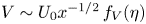 $V\sim U_0x^{-1/2}\,f_V(\eta )$ and
 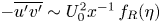 $-\overline {u'v'}\sim U_0^2x^{-1}\,f_R (\eta )$, where
  $f_U$,
  $f_V$,
  $f_R$ are transverse profiles. From data,
  $Max(f_U) =1$,
  $Max(f_V )<0.1$,
  $Max(f_R )<0.1$; and the profiles are
  $\approx 0$ for
  $\eta >2$ (HK65 and RC85). Hence
 $$\begin{gather} \left\vert{\frac{\partial}{\partial x} \int_{-\infty}^\infty UV \,{\rm d}\eta}\right\vert <\frac{U_0^2}{x^2} \int_{{-}2}^2 |\,f_Uf_V|_{Max} \,{\rm d}\eta < \frac{0.4U_0^2}{x^2}, \end{gather}$$
 $$\begin{gather}\left\vert\frac{\partial}{\partial x} \int_{-\infty}^\infty-\overline{u'v'} \,{\rm d}\eta\right\vert <\frac{U_0^2}{x^2} \int_{{-}2}^2 |\,f_R|_{Max} \,{\rm d}\eta < \frac{0.4U_0^2}{x^2}. \end{gather}$$
Classically, and from data, we know that  $\overline {v'^2}\approx ({0.05U_0^2}/{x})\,f_v^2(\eta )$ for
  $\eta < 2$. Hence
  $({\partial }/{\partial \eta })\,\overline {v'^2}\approx ({0.05U_0^2}/{x})\,({\partial f_v^2}/{\partial \eta }) \gg O({0.05U_0^2}/{x})$ because the transverse gradient
  ${\partial f_v^2}/{\partial \eta }$ is expected to be high. We also know that
  $|\Delta P| \approx \overline {v'^2}$ and
  $\overline {v'^2}\gg {V^2}$ inside the jet. The second term in equation (2.3), upon integrating across the jet at any given x, yields
  $|\Delta (V_{2} + \overline {v'^2} + P)|\sim 1/x$. Thus we estimate that the relative magnitude of the first term to the second term at streamwise distance
  $x$ is
 \begin{equation}
\frac{\left|\dfrac{\partial}{\partial x}
\displaystyle\int\nolimits_0^\infty (UV+\overline{u'v'})
\,{\rm d}\eta\right|} {\big|{\Delta} (V^2 + \overline{v'^2} + P)\big|} <
\frac{1}{x} \to 0 \quad\text{as}\ x\to \infty.
\end{equation}
\begin{equation}
\frac{\left|\dfrac{\partial}{\partial x}
\displaystyle\int\nolimits_0^\infty (UV+\overline{u'v'})
\,{\rm d}\eta\right|} {\big|{\Delta} (V^2 + \overline{v'^2} + P)\big|} <
\frac{1}{x} \to 0 \quad\text{as}\ x\to \infty.
\end{equation}


 Open access