


1. Introduction
Most current approaches to wall-bounded turbulence are based on momentum conservation and the concept of ‘momentum cascade’ to the wall (Tennekes & Lumley Reference Tennekes and Lumley1972; Jiménez Reference Jiménez2012; Yang, Marusic & Meneveau Reference Yang, Marusic and Meneveau2016). However, vorticity conservation may arguably be of equal or even greater importance. One of the earliest advocates of this point of view was Taylor (Reference Taylor1932), although his ‘vorticity transfer hypothesis’ was justly criticized for neglect of vortex stretching. Nevertheless, Taylor arrived at an important exact result that pressure drop in turbulent flow down a pipe is directly related to flux of spanwise vorticity across the flow. Lighthill (Reference Lighthill1963) was an even more forceful champion for vorticity-based approaches, positing that ‘to explain convincingly the existence of boundary layers …arguments concerning vorticity are needed’ and further that ‘vorticity considerations … illuminate the detailed development of the boundary layers just as clearly as do momentum considerations’. In particular, Lighthill (Reference Lighthill1963) argued that vorticity is uniquely suited to a causal description of fluid flows, as it is the only variable whose effects propagate at finite speeds in the incompressible limit.
Lighthill made in fact substantial concrete contributions to the program of explaining turbulent boundary layers by means of vorticity dynamics. One key idea introduced by Lighthill (Reference Lighthill1963), which is now widely recognized, is that vorticity generation at solid walls is due to tangential pressure gradients, with wall-normal vorticity flux given by
 \begin{equation} \boldsymbol{\sigma}=\boldsymbol{n}\times (\nu\boldsymbol{\nabla}\times \boldsymbol{\omega})={-}\boldsymbol{n}\times(\boldsymbol{\nabla}p+\partial_t \boldsymbol{u}), \end{equation}
 where u is the fluid velocity, ν is kinematic viscosity,  $\boldsymbol{\omega}$ is the vorticity, and
  $\boldsymbol {n}$ is the unit normal vector at the boundary pointing inward to the fluid. The term
  $\partial _t\boldsymbol {u}$ which accounts for tangential acceleration of the wall was introduced by Morton (Reference Morton1984), who emphasized further the inviscid character of such vorticity production. Although generally well accepted, the relations (1.1) have been the subject of some minor controversy, since they were first derived by Lighthill (Reference Lighthill1963) only for flat walls and were generalized subsequently to curved walls in the form (1.1) by Lyman (Reference Lyman1990) and in an alternative form
  $\boldsymbol {\sigma }'=-\nu (\boldsymbol {n}\boldsymbol {\cdot }\boldsymbol {\nabla })\boldsymbol {\omega }$ by Panton (Reference Panton1984). The subsequent debate over which of these two forms is ‘correct’ is reviewed by Terrington, Hourigan & Thompson (Reference Terrington, Hourigan and Thompson2021), who conclude that the two expressions measure slightly different things and have each their own (overlapping) domains of applicability. See also Wang, Eyink & Zaki (Reference Wang, Eyink and Zaki2022). Lyman's version (1.1) uniquely describes the creation of circulation at the boundary (Eyink Reference Eyink2008) and we use that form in our theoretical discussion here (but note the two coincide in our concrete application to channel flow). In either guise, the Lighthill source reveals that the solid walls are the ultimate origin of all vorticity in the flow, whereas for momentum the walls act instead as the sink. In consequence, the profound sensitivity of fluid flows to the nature of the solid boundary is better revealed by vorticity considerations.
Lighthill (Reference Lighthill1963) made another essential contribution to wall-bounded turbulence which seems, however, to have been less appreciated. To introduce Lighthill's basic insight, we can do no better than to quote at length from his own paper:
‘The main effect of a solid surface on turbulent vorticity close to it is to correlate inflow towards the surface with lateral stretching. Note that only the stretching of vortex lines can explain how during transition the mean wall vorticity increases as illustrated in figure II.21; and only a tendency, for vortex lines to stretch as they approach the surface and relax as they move away from it, can explain how the gradient of mean vorticity illustrated in figure II.21 is maintained in spite of viscous diffusion down it – to say nothing of any possible ‘turbulent diffusion’ down it, which the old ‘vorticity transfer’ theory supposed should occur. It is relevant to both these points that figure II.21 relates to uniform external flow, which implies zero mean rate of production of vorticity at the surface; but, even in an accelerating flow, the rate of production  $UU'$ is too small to explain either.
A simplified illustration of how inflow towards a wall tends to go with lateral stretching, and how outflow with lateral compression, is given in figure II.22. Doubtless some longitudinal deformation is usually also present, which reduces the need for lateral deformation (perhaps, on average, by half). However, there is evidence (from attempts to relate different types of theoretical model of a turbulent boundary layer to observations by hotwire techniques; see, for e.g. Townsend Reference Townsend1956) that the larger-scale motions (which push out ‘tongues’ of rotational fluid discussed above) are elongated in the stream direction, as if their vortex lines had been stretched longitudinally by the mean shear; in such motions, the correlation between inflow and lateral stretching illustrated in figure II.22 would be particularly strong. We may think of them as constantly bringing the major part of the vorticity in the layer close to the wall, while intensifying it by stretching and, doubtless, generating new vorticity at the surface; meanwhile, they relax the vortex lines which they permit to wander into the outer layer. Smaller-scale movements take over from these to bring vorticity still closer to the wall, and so on. Thus, the ‘cascade process’, which in free turbulence (see, for e.g. Batchelor Reference Batchelor1953) continually passes the energy of fluctuations down to modes of shorter and shorter length-scale – because at high Reynolds numbers motions in a whole range of scales may be unstable, which implies that motions of smaller scale can extract energy from them – this cascade process has the additional effect in a turbulent boundary layer of bringing the fluctuations into closer and closer contact with the wall, while their vortex lines are more and more stretched’. – From Lighthill (Reference Lighthill1963), pp. 98–99.
We find in this remarkable passage four key ideas: (i) first, the correlation between turbulent inflow and lateral vortex stretching illustrated by Lighthill (Reference Lighthill1963) with his figure II.22 acts to magnify principally spanwise vorticity and to drive it nearer the wall, as shown in his figure II.21 (both reproduced here as our figure 1). Conversely, turbulent outflow is correlated with lateral vortex compression, weakening the mainly spanwise vorticity as it is carried away from the wall. Quoting again from Lighthill (Reference Lighthill1963, p. 96), ‘it concentrates most of the vorticity much closer to the wall than before, although at the same time allowing some straggling vorticity to wander away from it farther’. The validity of this mechanism for a transitional boundary-layer flow has been verified recently by Wang et al. (Reference Wang, Eyink and Zaki2022). One would expect on the basis of this argument to find spanwise-extended vortex structures as principal elements of wall-bounded turbulent flows. (ii) The mechanism of correlated inflow/outflow and vortex stretching/contraction strongly sharpens vorticity gradients, acting against both viscosity and ‘eddy-viscosity’ effects which attempt to smooth the very sharp gradients created near the wall. As remarked by Lighthill (Reference Lighthill1963, p. 96), ‘turbulence redistributes the vorticity in such a way that viscous diffusion becomes more effective in countering the amplitude of the disturbances’. (iii) This intense competition between up-gradient flux on the one hand, and diffusion away from the wall by molecular and turbulence effects on the other, is narrowly won by the latter, since the net vorticity produced at the wall by the Lighthill source (1.1) must be transferred away under statistically steady conditions. Note that Lighthill's argument presumes that the total pressure  $p+(1/2)|\boldsymbol {u}|^2$ is continuous across accelerating turbulent boundary layers, so that the mean vortex production at the wall with steady, external mean velocity
  $U=\langle u\rangle$ is given by
  $U\partial _x U.$ (iv) Finally, Lighthill saw this up-gradient transport of vorticity toward the wall as a scale-by-scale cascade process, proceeding by the successive stretching, straightening and strengthening of spanwise vorticity through a hierarchy of eddy scales. Among the chief results of the present work will be extensive evidence in support of these insights of Lighthill.
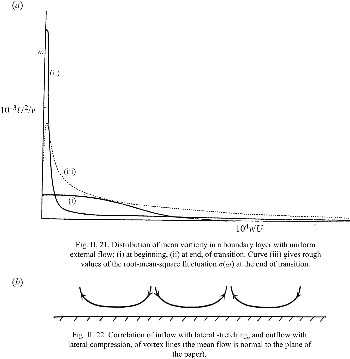
Figure 1. From M. J. Lighthill, ‘Introduction: Boundary layer theory’, in: Laminar Boundary Theory, Ed. L. Rosenhead, pp. 46–113. Copyright © 1963 by Oxford University Press. Reproduced with permission of the Licensor through PLSclear.
Closely related ideas were developed somewhat after Lighthill's work in the adjacent field of quantum superfluids, where Josephson (Reference Josephson1965) for superconductors and Anderson (Reference Anderson1966) for neutral superfluids recognized the relation between drops of voltage/pressure in flow through wires/channels and the cross-stream flux of quantized magnetic-flux/vortex lines. Their ideas closely mirror those of Taylor (Reference Taylor1932) and Lighthill (Reference Lighthill1963) for classical fluids, but Josephson (Reference Josephson1965) and Anderson (Reference Anderson1966) were seemingly unaware of those earlier works and the two literatures have subsequently developed in parallel. In quantum superfluids the Josephson–Anderson relation has become the paradigm to explain drag and dissipation in otherwise ideal superflow (Packard Reference Packard1998; Varoquaux Reference Varoquaux2015). This understanding is based in particular on the work of Huggins (Reference Huggins1970), who derived a ‘detailed Josephson–Anderson relation’ that exactly relates energy dissipation to vortex motions. Interestingly, although the target application of Huggins (Reference Huggins1970) was quantum superfluids, his mathematical model was the incompressible Navier–Stokes equation for a classical viscous fluid. In fact, somewhat later, Huggins (Reference Huggins1994) applied his ideas to classical turbulent channel flow.
More precisely, Huggins (Reference Huggins1970, Reference Huggins1994) considered a classical incompressible fluid at constant density  $\rho$ and with kinematic viscosity
  $\nu$ flowing in a channel with accelerations due both to a conservative force
  $-\boldsymbol {\nabla } Q$ and to a non-conservative force
  $-\boldsymbol {g}$ (with
  $\boldsymbol {\nabla } \boldsymbol {\times }\boldsymbol {g} \neq \boldsymbol {0}$), described by
 \begin{equation} \partial_t\boldsymbol{u}=\boldsymbol{u}\times \boldsymbol{\omega} -\nu\boldsymbol{\nabla}\boldsymbol{\times}\boldsymbol{\omega}- \boldsymbol{\nabla}(p/\rho+|\boldsymbol{u}|^2/2+Q )-\boldsymbol{g}.\end{equation}
For example,  $Q$ might be the gravitational potential energy density
  $\rho g y$ for vertical height
  $y$ (with acceleration due to gravity
  $g$), and
  $\boldsymbol {g}$ might be
  $-\boldsymbol {\nabla }\boldsymbol {\cdot }\boldsymbol {\tau }_p$ with
  $\boldsymbol {\tau }_p$ the stress of a polymer additive. Huggins (Reference Huggins1970, Reference Huggins1994) noted that this equation for the momentum balance may be rewritten as
 \begin{equation} \partial_tu_i=(1/2)\epsilon_{ijk}\varSigma_{jk}-\partial_i h,\end{equation}
with anti-symmetric vorticity flux tensor
 \begin{equation} \varSigma_{ij} = u_i\omega_j-u_j\omega_i +\nu\left(\frac{\partial\omega_i}{\partial x_j}-\frac{\partial\omega_j}{\partial x_i}\right)-\epsilon_{ijk}g_k, \end{equation}
and total pressure or enthalpy
 \begin{equation} h=p/\rho+|\boldsymbol{u}|^2/2+Q. \end{equation}
Here, the total pressure h includes both the hydrostatic and the dynamic pressures, and the tensor  $\varSigma _{ij}$ represents the flux of the jth vorticity component in the ith coordinate direction. The latter interpretation is made clear by taking the curl of the momentum equation (1.2), which yields a local conservation law for vector vorticity
 \begin{equation} \partial_t\omega_j+\partial_i\varSigma_{ij} =0. \end{equation}
The first term in (1.4) for  $\varSigma _{ij}$ represents the advective transport of vorticity, the second represents transport by nonlinear stretching and tilting, the third represents viscous transport and the fourth represents transport of vorticity perpendicular to an applied, non-conservative body force
  $\boldsymbol {g}$ akin to the Magnus effect. The stretching/tilting term
  $(\boldsymbol {\omega }\boldsymbol {\cdot }\boldsymbol {\nabla })\boldsymbol {u}$ in the Helmholtz equation violates material conservation, so that
  $D_t\boldsymbol {\omega }\neq 0,$ but it can nevertheless be written as a total divergence
  $\boldsymbol {\nabla }\boldsymbol {\cdot }(\boldsymbol {\omega }\boldsymbol {u})$ and thus interpreted as a space transport of vorticity (see § 2). Equation (1.3) thus shows the deep connection between momentum balance and vorticity transport, and this equation is the most elementary version of the classical Josephson–Anderson relation; see also the insightful study of Brown & Roshko (Reference Brown and Roshko2012) in the context of flow past a cylinder and the more recent work of Terrington et al. (Reference Terrington, Hourigan and Thompson2021), who discuss at length the meaning and applications of the anti-symmetric vorticity flux tensor (1.4), which they call the ‘Lyman–Huggins tensor’.
A first attempt was made by Eyink (Reference Eyink2008) to unify these parallel theories in the context of two canonical turbulent flows, plane-parallel channels and straight pipes. He discussed the physical significance of the observation by Taylor (Reference Taylor1932) and by Huggins (Reference Huggins1994) that there is a mean cross-stream vorticity flux driven by the downstream pressure gradient. In the context of channel flow, with  $x$ the streamwise direction,
  $y$ the wall-normal direction and
  $z$ the spanwise direction, this average relation takes the form
 \begin{equation} \langle \varSigma_{yz}\rangle =\langle v\omega_z- w\omega_y-\nu(\partial_y\omega_z-\partial_z\omega_y)\rangle= \partial_x \langle p\rangle={-}u_\tau^2/h, \end{equation}
where  $\varSigma _{yz}$ is the wall-normal flux of spanwise vorticity,
  $h$ is the channel half-height and
  $u_{\tau }$ is the friction velocity. The standard result that
  $\partial _y\partial _x \langle p\rangle =0$ (Tennekes & Lumley Reference Tennekes and Lumley1972, § 5.2) is seen to be a consequence of vorticity conservation
  $\partial _y\langle \varSigma _{yz}\rangle =0.$ Eyink (Reference Eyink2008) noted that Huggins’ vorticity flux tensor (1.4) and Lighthill's vorticity source (1.1) in the form of Lyman (Reference Lyman1990) are simply related by
  $\boldsymbol {\sigma }= \boldsymbol {n} \boldsymbol {\cdot } \boldsymbol {\varSigma },$ so that the origin of the constant mean flux is the vorticity created at the wall, which flows toward the channel centre to be annihilated by opposite-sign vorticity from the facing wall. Eyink (Reference Eyink2008) referred to this phenomenon as an ‘inverse vorticity cascade’, but note that the vorticity transport involved here is down-gradient, opposed by the up-gradient cascade mechanism proposed by Lighthill (Reference Lighthill1963). The term ‘inverse cascade’ was used by Eyink (Reference Eyink2008) because the mean vorticity flux is in the opposite direction as the mean flux of momentum, that is, out from the wall and via eddies of increasing size at further distances from the wall. Just as spatial momentum flux in wall-bounded turbulence can be interpreted as a stepwise cascade (Tennekes & Lumley Reference Tennekes and Lumley1972; Jiménez Reference Jiménez2012), so also spatial vorticity transport can be understood as a cascade through a hierarchy of eddies whose sizes scale with distance to the wall.
A possible mechanism for this cascade is lifting and growing hairpin-like vortex structures in the inertial sublayer of the channel flow. It was shown by Eyink (Reference Eyink2008) that constant mean down-gradient flux of vorticity via the nonlinear dynamics can in fact be explained by the attached-eddy model (AEM) of Townsend (Reference Townsend1976) (see Marusic & Monty (Reference Marusic and Monty2019) for a recent comprehensive review). Since the AEM is not designed to describe the statistics and dynamics of the fine-grained vorticity (Marusic & Monty Reference Marusic and Monty2019, § 4.1), it is not entirely trivial that the model should account for the mean vorticity flux. However, this flux can be deduced from the Reynolds stress by the standard relation (Taylor Reference Taylor1915; Tennekes & Lumley Reference Tennekes and Lumley1972; Klewicki Reference Klewicki1989)
 \begin{equation} \langle v \omega_z- w\omega_y\rangle ={-}\partial_y\langle u'v'\rangle, \end{equation}
from which it can be shown that the AEM implies  $\langle v\omega _z-w\omega _y\rangle \sim -u_\tau ^2/h$ for
  $y\gtrsim y_p,$ where
  $y_p$ is the wall distance of the peak Reynolds stress (Eyink Reference Eyink2008). On the contrary, for
  $y< y_p$ it follows directly from (1.8) that
  $\langle v\omega _z- w\omega _y\rangle >0,$ whose positive sign indicates up-gradient nonlinear transport of (negative) spanwise vorticity. It was noted by Eyink (Reference Eyink2008) that this up-gradient transport is not obviously explained by attached eddies and we shall present here strong evidence that the underlying mechanism is in fact that of Lighthill (Reference Lighthill1963). A further impetus to our investigation comes from recent work of Eyink (Reference Eyink2021), who showed that the ‘detailed relation’ of Huggins (Reference Huggins1970) for energy dissipation in channel flows holds also for flow around a uniformly moving solid body. In fact, this result holds much more generally for bodies that are moving non-uniformly and even changing shape and volume (Eyink, unpublished) and also for channel flows with periodic boundary conditions (Kumar & Eyink, unpublished). In all of these situations, there is flux of vorticity away from the solid surface and net drag is given instantaneously by the spatial integral of spanwise vorticity flux across the streamlines of a background potential Euler flow.
To gain further insight into the underlying fluid-dynamical mechanisms of turbulent vorticity cascade, we here carry out a detailed investigation of the turbulent vorticity dynamics in the simplest case of turbulent channel flow. Although viscous diffusion plays a dominant role in the mean vorticity transport out to the wall distance  $y_p$ (Klewicki et al. Reference Klewicki, Fife, Wei and McMurtry2007; Eyink Reference Eyink2008; Brown, Lee & Moser Reference Brown, Lee and Moser2015), its properties follow directly from the mean velocity profile and are thus relatively easy to understand. We shall therefore be more concerned with the nonlinear vorticity dynamics and the resulting statistics of the velocity–vorticity correlations
  $\langle v \omega _z\rangle,$
  $\langle w\omega _y\rangle$ at various wall distances. We employ data for our study from the Johns Hopkins Turbulence database (JHTDB) which stores the output of a direct numerical simulation (DNS) of turbulent channel flow at friction Reynolds number
  $Re_{\tau }=1000$ (Li et al. Reference Li, Perlman, Wan, Yang, Meneveau, Burns, Chen, Szalay and Eyink2008; Graham et al. Reference Graham2016). This simulation was performed using the petascale DNS channel-flow code PoongBack (Lee, Malaya & Moser Reference Lee, Malaya and Moser2013) with driving force provided by a constant applied pressure gradient. The resulting online database archives full space–time fields of velocity and pressure throughout the channel domain and for about one flow-through time. The archived data permit us to calculate not only the velocity–vorticity correlations but also their Fourier cospectra in streamwise wavenumber
  $k_x,$ spanwise wavenumber
  $k_z$ and two-dimensional (2-D) wavenumber
  $(k_x,k_z),$ which prove particularly illuminating of the physics.
It is important to emphasize once again the dual role of the quantity  $(\boldsymbol {u}\times \boldsymbol {\omega })_x =v \omega _z- w\omega _y$ that is studied in this work. On the one hand, it is the streamwise component of the ‘vortex force’ which appears in the momentum balance (1.2), while on the other hand it is the inertial contribution to the component
  $\varSigma _{yz}$ of the conserved vorticity current. Much prior work has focused on the role of the mean vortex force
  $\langle v\omega _z-w\omega _y \rangle =\langle v'\omega _z'-w'\omega _y' \rangle$, interpreted as a ‘turbulent inertia’ (TI) term through (1.8). Separate contributions
  $\langle v'\omega _z'\rangle$ and
  $\langle w'\omega _y'\rangle$ were measured experimentally by Klewicki (Reference Klewicki1989) and weighted joint probability density functions (p.d.f.s) of
  $v',\omega _z'$ and of
  $u',\omega _z'$ were obtained by Klewicki, Murray & Falco (Reference Klewicki, Murray and Falco1994). A four-layer structure for wall-bounded flows was proposed by Wei et al. (Reference Wei, Fife, Klewicki and McMurtry2005), based on the relative magnitude of the viscous and TI term in the mean momentum equation (see also Klewicki et al. Reference Klewicki, Fife, Wei and McMurtry2007). The wall-normal derivatives of streamwise spectra of the Reynolds shear stress, equal to the nonlinear flux cospectra for periodic flows, were studied as ‘net force spectra’ for pipe flows (Guala, Hommema & Adrian Reference Guala, Hommema and Adrian2006) and for channel flows and zero-pressure-gradient boundary layers (Balakumar & Adrian Reference Balakumar and Adrian2007). An in-depth study of the statistics and streamwise spectral behaviour of the velocity–vorticity products for turbulent boundary layers, at several
  $Re$ values, was carried out by Priyadarshana et al. (Reference Priyadarshana, Klewicki, Treat and Foss2007). They compared streamwise spectra for velocity and vorticity with the corresponding cospectra and plotted profiles of the velocity–vorticity products and correlation coefficients. The correlations between velocity and vorticity were seen to arise from a ‘scale selection’ associated with peaks in the velocity and vorticity streamwise spectra. Monty, Klewicki & Ganapathisubramani (Reference Monty, Klewicki and Ganapathisubramani2011) interpret the TI term as a momentum source/sink (depending upon the sign) and carried out detailed calculations of the streamwise and spanwise two-point correlations of
  $v$ with
  $\omega _z$ and
  $w$ with
  $\omega _y$ in a DNS of channel flow. They drew an important conclusion, which anticipates our own, that ‘the mean Reynolds stress gradient at any wall-normal location is a direct result of a slight asymmetry in the characteristic vortical motions of the flow’. The work of Wu, Baltzer & Adrian (Reference Wu, Baltzer and Adrian2012), primarily studied streamwise very large-scale motions and their relations to shear stress in DNS of pipe flows, but they computed as well 2-D ‘net force spectra’ jointly in streamwise and spanwise wavenumbers at four wall-normal locations, scaled with outer units. Morrill-Winter & Klewicki (Reference Morrill-Winter and Klewicki2013) carried out experimental investigations for flat plate boundary layers, studying streamwise cospectra, scale selection, two-point correlations and Reynolds number effects. Chin et al. (Reference Chin, Philip, Klewicki, Ooi and Marusic2014) made a detailed analysis of the TI term for DNS of pipe flows, decomposing it into advective transport and vorticity stretching/tilting and studying wall-normal variation of the respective streamwise cospectra and the combined ‘net force spectrum’, as well as joint p.d.f.s of
  $v',\omega _z'.$
A smaller body of work has studied velocity–vorticity correlations instead as the nonlinear contribution to mean vorticity flux, following the early work of Taylor (Reference Taylor1915, Reference Taylor1932), including the DNS studies of Bernard (Reference Bernard1990), Crawford & Karniadakis (Reference Crawford and Karniadakis1997) and Vidal, Nagib & Vinuesa (Reference Vidal, Nagib and Vinuesa2018). In DNS of channel flows over a range of Reynolds numbers, Brown et al. (Reference Brown, Lee and Moser2015) studied vorticity flux, highlighting the fact that its mean is constant across every wall-parallel plane for a turbulent pressure-driven channel flow and evaluating the two nonlinear contributions. Of particular interest is their calculation of the p.d.f.s of  $w\omega _y$ close to the wall and their visualization of the vortex lines passing through such a region. Experimental measurements for an open channel flow by Chen et al. (Reference Chen, Adrian, Zhong, Li and Wang2014) focused on the contributions of spanwise vortex filaments to Reynolds shear stress and to
  $v\omega _z$. Apart from measuring separate contributions to the advection term from prograde and retrograde vortices, they observed that the movement away from the wall yields the significant contribution of spanwise vortex filaments (identified by a swirling strength-based criterion) to the ‘net force’. These ideas were further explored in Chen et al. (Reference Chen, Li, Bai and Wang2018b), where flow structures were classified into four groups based on vorticity and swirling strength, and contributions made by these structures to the nonlinear vorticity fluxes were measured.
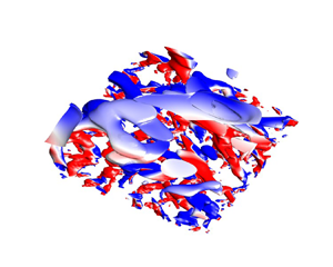
A key contribution of our work, which distinguishes it from all of the previous studies cited above, is to make a clear connection of our numerical results with the ideas of Lighthill (Reference Lighthill1963) which focus on vorticity dynamics. Based on new theoretical insights and novel analysis of data using conditional averaging, we shall argue that Lighthill's theory provides a compelling explanation of many prior observations. Furthermore, by a targeted filtering based upon joint velocity–vorticity cospectra, we show that Lighthill's ‘up-gradient’ vorticity cascade involves a previously unidentified hierarchy of non-attached, near-wall eddies, with important implications for theory and modelling.
The detailed contents of this paper are outlined as follows. In § 2 we discuss how Lighthill's Lagrangian mechanism is represented by the Eulerian vorticity flux tensor, a necessary theoretical prelude so that our subsequent numerical results can be appropriately interpreted. The main § 3 of the paper presents our numerical study. In § 3.1 we study the mean vorticity flux and its component velocity–vorticity correlations, validating our own numerical results against previously published results and illustrating the mean flow of vorticity along isolines of total pressure. The next § 3.2 presents results on conditional averages of fluxes given the direction of the wall-normal velocity as inward or outward, in order to investigate the proposed strong correlation. Section 3.3 presents results on cospectra of the nonlinear vorticity flux and velocity–vorticity correlations, both 1-D spectra in the streamwise and spanwise wavenumbers and joint 2-D spectra. Then in § 3.4 we use the 2-D cospectra to divide the velocity and vorticity fields into ‘down-gradient’ and ‘up-gradient’ eddy contributions and we visualize the coherent vortices which dominate transport in both of these components. Finally, in the conclusion § 4 we review our main results, draw relevant lessons and discuss important future directions. Incidental numerical results of various sorts are presented in supplementary materials (available at https://doi.org/10.1017/jfm.2023.609).
2. The Lighthill mechanism and Huggins’ vorticity flux tensor
In order to properly interpret the results of our numerical study, we must first discuss carefully the physical and mathematical meaning of Lighthill's arguments. This is necessary especially because Lighthill's dynamical picture is essentially Lagrangian whereas Huggin's vorticity flux tensor (1.4) is Eulerian. Thus, the relation between Lighthill's mechanism and the predicted behaviour of Huggins’ flux can be somewhat subtle and even counter-intuitive.
The basic picture behind Lighthill's argument is sketched as a cartoon in figure 2. Shown there is a representative vortex line carrying spanwise vorticity and also wall-normal vorticity associated with a lifted arch. If the flow is inward toward the wall ( $v<0$) at this location, then, by incompressibility, there must be diverging flow in the spanwise and/or streamwise directions. See figure 2(a). This divergent flow should generate corresponding velocity gradients in those directions which Lighthill argued should be strongest spanwise because the well-known longitudinal organization of the near-wall structures would tend to reduce streamwise gradients. According to the Helmholtz laws of ideal vortex dynamics, one would therefore expect the vortex line to be, first, carried down by the flow closer to the wall and, second, flattened and stretched out, principally in the spanwise direction. This action of the Lagrangian flow is indicated by the blue dashed arrows in figure 2(a) which depict typical particle trajectories. Since the stretched vortex line should intensify, Lighthill suggested that the plausible result would be increased spanwise vorticity concentrated closer to the wall. The opposite effect should occur in regions of flow outward from the wall (
 $v>0$), which corresponds to the same cartoon but reversing all velocity vectors given by red arrows and all Lagrangian trajectories given by blue dashed lines. See figure 2(b). In this case the vortex line according to ideal laws would be lifted away from the wall, compressed in the spanwise direction and correspondingly weakened. Such motions, according to Lighthill, would reduce the spanwise vorticity at further distances from the wall, so that the net effect of both types of motion would be an increase in the intensity of vorticity at the wall and a steepening of its wall-normal gradient. However, note that, according to the Kolmogorov theory of local isotropy (Tennekes & Lumley Reference Tennekes and Lumley1972), streamwise and spanwise velocity gradients may be of a similar magnitude at small enough scales. Therefore, the association of inflow/outflow with stretching/relaxing of spanwise aligned vortex lines is expected to be primarily valid at scales that are large enough to possess the streamwise organization associated with stronger spanwise gradients.
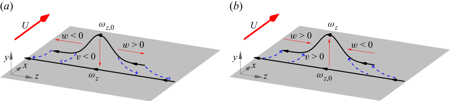
Figure 2. Cartoon of Lighthill's Lagrangian mechanism (‘vortex lines … stretch as they approach the surface and relax as they move away from it’) for typical vortex lines in the buffer and log layers. (a) Inflow and vortex stretching,  $|\omega _{z}|>|\omega _{z,0}|$; (b) outflow and vortex compression,
  $|\omega _{z}|<|\omega _{z,0}|$. In both cases, initial vorticity is given by
  $\omega _{z,0}$ and final vorticity by
  $\omega _z$.
An obvious concern with this picture is its neglect of viscous diffusion effects, which certainly must be substantial in the near-wall buffer layer and viscous sublayer. In fact, as noted above, viscous diffusion dominates the average wall-normal flux of spanwise vorticity out to the location  $y_p$ of peak Reynolds stress (Klewicki et al. Reference Klewicki, Fife, Wei and McMurtry2007; Eyink Reference Eyink2008; Brown et al. Reference Brown, Lee and Moser2015). The viscous modifications of ideal vortex dynamics can be incorporated by means of a stochastic Lagrangian formulation of incompressible Navier–Stokes in vorticity–velocity representation (Constantin & Iyer Reference Constantin and Iyer2011; Eyink, Gupta & Zaki Reference Eyink, Gupta and Zaki2020a), which represents viscous diffusion of vorticity by an average over stochastic Brownian perturbations of Lagrangian particle motions. This approach was exploited by Wang et al. (Reference Wang, Eyink and Zaki2022) to investigate the origin of the enhanced wall vorticity and skin friction in a transitional zero-pressure-gradient boundary layer, as discussed in the passage from Lighthill (Reference Lighthill1963) quoted in the Introduction. This study used the Lighthill vorticity source
  $\boldsymbol {\sigma }$ in (1.1) as Neumann boundary conditions, so that the wall vorticity at points of local maximum amplitude could be expressed in terms of two contributions: (i) the Lighthill source integrated over earlier times and (ii) the initial conditions for the vorticity as modified by subsequent advection, stretching and viscous diffusion. It was found that the dominant source of the high wall vorticity is the spanwise stretching of pre-existing spanwise vorticity, exactly as argued by Lighthill (Reference Lighthill1963). In particular, as also suggested by Lighthill, the rate of production by the vorticity source
  $\boldsymbol {\sigma }$ was ‘too small to explain’ the maxima. This contribution was found in general to be about an order of magnitude smaller than that from spanwise stretching and also found to give vorticity contributions of both signs with about equal probability, thus often reducing the magnitude. The conclusion of Wang et al. (Reference Wang, Eyink and Zaki2022) from their analysis of the numerical data was that, despite strong viscous effects in the near-wall region, the theory of Lighthill (Reference Lighthill1963) explained well the origin of high wall-stress events observed in transitional flow.
The same stochastic Lagrangian methods can be applied also to fully developed turbulent channel flow, but here, motivated by recent work of Eyink (Reference Eyink2021) and Kumar & Eyink (unpublished) on the Josephson–Anderson relation, we instead aim to understand the vorticity dynamics in terms of Huggins’ vorticity current tensor (1.4). Because the vorticity conservation law (1.6) is expressed in Eulerian form, its relationship to Lighthill's Lagrangian picture is not entirely self-evident. The physical meaning of Huggins’ tensor  $\varSigma _{ij}$ has previously been discussed by Terrington et al. (Reference Terrington, Hourigan and Thompson2021) and Terrington, Hourigan & Thompson (Reference Terrington, Hourigan and Thompson2022) using control volumes and control surfaces. To adapt their arguments, we integrate (1.6) over a volume
  $V$ to obtain
 \begin{equation} \frac{{\rm d}}{{\rm d}t} \int_V \omega_j \,{\rm d}^3x ={-}\oint_{\partial V} n_i\varSigma_{ij} \,{\rm d}A , \end{equation}
where  $\boldsymbol {n}$ is the outward-pointing normal at the boundary
  $\partial V$ and each individual term in
  $n_i\varSigma _{ij}$ should represent a rate of change of
  $\omega _j$ integrated over
  $V.$ The meaning of the nonlinear term
  $u_i\omega _j$ is transparent, as
  $(\boldsymbol {n}\boldsymbol {\cdot }\boldsymbol {u})\omega _j$ just represents the advection of
  $\omega _j$ across the boundary
  $\partial V.$ The other nonlinear contribution
  $-u_j\omega _i$ to the flux upon taking its divergence yields the term
  $-(\boldsymbol {\omega }\boldsymbol {\cdot }\boldsymbol {\nabla })\boldsymbol {u}$ in the Helmholtz equation associated with vortex stretching and tilting, so that it must somehow express that physics. It is worth remarking that Huggins (Reference Huggins1994, p. 326), concluded that this term ‘does not appear to have a particularly simple interpretation’ but suspected that it is ‘a vortex stretching term’. The relation with stretching/tilting is clarified by figure 3(a), which plots schematically the first ‘up-gradient’ configuration considered by Lighthill (Reference Lighthill1963) with flow inward to the wall advecting and stretching/tilting a hairpin-like vortex. We have drawn as control volume a rectangular box selected so that only the term
  $-w\omega _y$ in the flux
  $\varSigma _{yz}$ contributes to growth of spanwise vorticity
  $\omega _z$ in the volume, whereas the advection term
  $v\omega _z$ does not contribute. Because of the diverging flow, two contributions with signs
  $\omega _y>0,$
  $w>0$ and
  $\omega _y<0,$
  $w<0$ occur at the bottom face of the box and these correspond indeed to an increase of (negative) spanwise vorticity in the pictured control volume, due to the lengthening of the spanwise vortex line segment and the tilting of the wall-normal vortex line segments. It is notable that the contribution
  $-w\omega _y<0$ at the bottom face in figure 3(a) corresponds to an outward flux of spanwise vorticity into the control volume, with a sign which is formally ‘down-gradient’ or away from the wall. By contrast, the advection term has sign
  $v\omega _z>0$ which is ‘up-gradient’ and from Lighthill's Lagrangian argument we may expect that the net nonlinear transfer is ‘up-gradient’ for this flow configuration with
  $v<0$. If we consider instead the outward flow configuration with
  $v>0$ illustrated in figure 3(b), which compresses and weakens the spanwise vorticity, then the signs would both reverse to
  $v\omega_z<0$ and
  $-w\omega_y>0$ (because of converging flow), but would remain opposite. The advective term is now making a ‘down-gradient’ contribution and the stretching/tilting term is making an ‘up-gradient’ contribution, with the net nonlinear flux expected to be ‘up-gradient’.

Figure 3. Eulerian control-volume analysis of the same vorticity dynamics illustrated in figure 2. (a) Inward flow ( $v<0$) and (b) outward flow (
 $v>0$). The control volumes are chosen to highlight the contribution of the stretching/tilting term to the change of integrated
  $\omega _z$ in the volume by flux across the bottom face.
To determine whether the net vorticity flux from nonlinearity is ‘up-gradient’ or ‘down gradient’, it is important consider the combined term  $u_i\omega _j-u_j\omega _i,$ which is anti-symmetric. As stressed by Terrington et al. (Reference Terrington, Hourigan and Thompson2021), the anti-symmetry
  $\varSigma _{ji}=-\varSigma _{ij}$ expresses the fundamental property that vortex lines cannot end in the fluid so that flux of
  $\omega _j$ in the
  $i$th direction is necessarily associated with an equal and opposite flux of
  $\omega _i$ in the
  $j$th direction. This relation of flux anti-symmetry and non-termination of vortex lines is clearly illustrated in figure 3(a), for example. In the flow sketched there, the depicted spanwise flux
  $\varSigma _{zy}$ of
  $\omega _y$-vorticity implies that the
  $\omega _z$-line must lengthen, because the vortex line which enters at one
  $z$-location in the bottom face must exit at the other. The resulting growth of
  $\omega _z$-vorticity in the interior by stretching and tilting corresponds to a wall-normal flux
  $\varSigma _{yz}=-\varSigma _{zy}$ outward into the control volume. To determine from our numerical data whether nonlinear flux of spanwise vorticity is ‘down-gradient’ or ‘up-gradient’ it will therefore be crucial to consider the combined quantity
  $v\omega _z-w\omega _y$ that contains both advection and stretching/tilting, since these two effects cannot be separated physically without violating the kinematic condition of non-terminating vortex lines.
The anti-correlated sign of the two separate flux contributions from advection and stretching/tilting will be crucial, on the other hand, in interpreting our numerical results below, since this anti-correlation is a key Eulerian signature of Lighthill's mechanism. Figure 3(a) shows that the strengthening of spanwise vorticity during an inflow is represented in the Eulerian flux by a ‘down-gradient’ stretching/tilting term, even though the net flux is ‘up-gradient’. Similarly, figure 3(b) shows that the weakening of spanwise vorticity during an outflow is represented in the Eulerian flux by an `up-gradient' stretching/tilting term, even though the net flux is ‘down-gradient’. This anti-correlation of the stretching/tilting term with the net flux is thus a direct manifestation of Lighthill's mechanism. It should be clear that this anti-correlation of signs depends upon the geometry of the vortex line. For example, if the vortex line in figure 3(a) were instead bent inward into a U-shape and entered the control volume from the top face, then the sign of the stretching/tilting term would have become  $-w\omega _y>0.$ This inward flux into the control volume would again correspond to vortex strengthening, but it would now represent formally ‘up-gradient’ transport positively correlated with the advection term
  $v\omega _z>0.$ Because of the assumption of a specific vortex line geometry in figure 3, the suggested anti-correlation between the signs of the advection and stretching/tilting terms can be claimed only to be consistent with Lighthill's ideas, which should be further investigated. More positively, the relative sign of the advection term and of the stretching/tilting term potentially contains some information about the typical geometry of vortex lines.
3. Numerical study of vorticity flux in pressure-driven channel flow
We now report on our empirical study of the flux of spanwise vorticity, hereafter referred to simply as ‘vorticity flux’. This component of the vorticity is crucial to drag and energy dissipation, since its flux is directly related to streamwise pressure drop. As already mentioned in the Introduction (§ 1), we employ DNS data of channel flow at  $Re_{\tau }=1000$ from the JHTDB (see Li et al. Reference Li, Perlman, Wan, Yang, Meneveau, Burns, Chen, Szalay and Eyink2008; Graham et al. Reference Graham2016). The right-handed Cartesian coordinate system for these data is the same as shown in figures 2 and 3(a), with
  $x$ streamwise,
  $y$ wall-normal and
  $z$ spanwise. Although the database provides built-in tools to calculate velocity and vorticity gradients from Lagrange interpolants, our study of vorticity dynamics required greater accuracy for these crucial quantities. We have thus used the database cut-out service to download time snapshots of data for the entire channel. Gradients in the spanwise and streamwise directions are then calculated spectrally by Fast Fourier Transform, and wall-normal gradients are calculated using seventh-order basis splines based on the collocation points of the original simulation (Graham et al. Reference Graham2016). All statistics are thereafter calculated by averaging over wall-parallel planes in the
  $x$- and
  $z$-directions of homogeneity, as well as over multiple snaphots. The steady-state statistics presented here were calculated with 38 time snaphots. We shall generally plot our results only for the bottom half of the channel, with reflected results from the top half included to double the sample size of our averages.
3.1. Mean vorticity flux and flow lines
To provide an intuitive understanding of Huggins’ vorticity flux tensor (1.4) and of the mean vorticity dynamics in turbulent channel flow, we first present numerical results on the average flux  $\langle \varSigma _{ij}\rangle.$ An important theoretical result which follows directly by averaging the momentum balance equation (1.3) is the steady-state relation between vorticity flux and the gradients of the total pressure
 \begin{equation} \langle \varSigma_{ij}\rangle = \epsilon_{ijk}\partial_k\langle h\rangle. \end{equation}
This general result implies immediately for channel flow that
 \begin{equation} \langle\varSigma_{yz}\rangle=\partial_x\langle h\rangle, \quad \langle\varSigma_{xz}\rangle={-}\partial_y\langle h\rangle, \quad \langle \varSigma_{xy}\rangle=0, \end{equation}
with all other components given by anti-symmetry. Since it is the flux of spanwise vorticity only which enters into the Josephson–Anderson relation for plane-parallel channel flow (Kumar & Eyink, unpublished) we shall focus on its dynamics in the  $(x,y)$-plane (since
  $\varSigma _{zz}=0$). It can be very instructive about the physics to trace the integral flow lines of mean fluxes for transported quantities such as energy and momentum (Meyers & Meneveau Reference Meyers and Meneveau2013) and we carry out this construction for the conserved spanwise vorticity. Here, there is a substantial simplification because, as a simple consequence of (3.2a–c), the integral lines of the mean flux vector
  $(\langle \varSigma _{xz}\rangle,\langle \varSigma _{yz}\rangle )$ coincide with the isolines of mean total pressure
  $\langle h\rangle = P + \frac {1}{2}U^2 + \frac {1}{2}\langle |u'|^2+|v'|^2+|w'|^2\rangle.$ We follow the usual notations,
  $U=\langle u\rangle,$
  $u'=u-U,$
  $P=\langle p\rangle,$ etc. In figure 4 we plot these isolines resulting from numerical computation of
  $\langle h\rangle.$ Consistent with the remark of Lighthill (Reference Lighthill1963) that ‘tangential vorticity created is in the direction of the surface isobars’, the mean vorticity generated at the wall is spanwise and flows outward from points of constant
  $\langle h\rangle =P$ at
  $y=0.$ The vorticity flux is approximately three orders of magnitude larger streamwise than wall normal, mainly because of the large term
  $U\varOmega _z$ contributing to
  $\langle \varSigma _{xz}\rangle,$ with
  $\varOmega _z=-\partial _yU.$ Thus, the mean vorticity flow lines extend approximately 250 channel half-widths downstream as they cross from the wall to the channel centre, reflecting the strong streamwise advection of vorticity. It is, however, the much smaller wall-normal vorticity flux which is directly related to drag and energy dissipation, since
  $\langle \varSigma _{yz}\rangle =\partial _xP$ by (3.2a–c). As earlier remarked by Eyink (Reference Eyink2008), the latter takes on the
  $y$-independent value
  $\langle \varSigma _{yz}\rangle =-u_\tau ^2/H$ because of the conservation relation
  $\partial _y\langle \varSigma _{yz}\rangle = \partial _y\langle \varSigma _{yz}\rangle +\partial _x\langle \varSigma _{xz}\rangle =0$ and the Lighthill (Reference Lighthill1963) relation for wall generation of vorticity by tangential pressure gradients. This argument assumes as well the
  $x$-independence of steady-state averages such as
  $\langle \varSigma _{xz}\rangle$, which is evident in the parallel vorticity flux lines of figure 4.

Figure 4. Flow lines of mean spanwise vorticity flux  $(\langle \varSigma _{xz}\rangle,\langle \varSigma _{yz}\rangle )$ obtained as the isolines of mean total pressure
  $\langle h\rangle$.
Exact results of Klewicki et al. (Reference Klewicki, Fife, Wei and McMurtry2007), Eyink (Reference Eyink2008) and Brown et al. (Reference Brown, Lee and Moser2015) for the nonlinear  $\langle v\omega _z -w\omega _y \rangle$ and viscous
  $-\nu \langle \partial _y\omega _z-\partial _z\omega _y\rangle$ contributions to the mean vorticity flux
  $\langle \varSigma _{yz}\rangle$ provide a further check of the reliability of our numerics. Our numerical data are plotted in figure 5 and show good agreement with the theoretically required behaviour. First, we observe that the magnitude of the mean vorticity flux is constant in
  $y$ to a very good approximation, except for small numerical oscillations very close to the wall (
 $y^+<10$), and it matches quite well the average streamwise pressure gradient. This means that, on average, negative spanwise vorticity (the same sign as the mean vorticity) is being transported away from the wall and that overall, the flux is down-gradient. As in the Introduction, we shall refer to flux of vorticity away from the wall as ‘down-gradient’, since the vorticity is already highly concentrated at the wall (Lighthill Reference Lighthill1963), and flux in the opposite direction will be referred to as ‘up-gradient’. It was also shown by Klewicki et al. (Reference Klewicki, Fife, Wei and McMurtry2007), Eyink (Reference Eyink2008) and Brown et al. (Reference Brown, Lee and Moser2015) that, while viscous flux should be expected to be always down-gradient, the net nonlinear flux will be down-gradient above the height of the peak Reynolds stress (
 $y^+=y_p^+=53$ for the data at
  $Re_\tau = 1000$) but up-gradient below that height and opposing the large viscous flux there. These theoretical results are well confirmed by our empirical data in figure 5. In addition, we have calculated the separate contributions of the advective (
 $v\omega _z$) and stretching/tilting (
 $-w\omega _y$) terms to the nonlinear flux, for which no exact predictions exist. However, our results for these two quantities plotted also in figure 6 agree well with those earlier reported by Monty et al. (Reference Monty, Klewicki and Ganapathisubramani2011), Brown et al. (Reference Brown, Lee and Moser2015) and Chen et al. (Reference Chen, Li, Bai and Wang2018b) from the channel-flow simulation of Del Alamo et al. (Reference Del Alamo, Jiménez, Zandonade and Moser2004) at
  $Re_\tau =934$ and also with the experimental results of Chen et al. (Reference Chen, Adrian, Zhong, Li and Wang2014) for an open channel flume at somewhat lower
  $Re_\tau =740.$ Similar observations have been made both at lower and at higher Reynolds numbers, but we postpone until our conclusions section the discussion of the important issue of
  $Re$-dependences. Confirming those earlier studies, we find that both contributions are down-gradient in the outer range (
 $y^+\gtrsim 300$) and both up-gradient in the near wall (
 $y^+\lesssim 10$), but have opposite signs in the intermediate range corresponding roughly to the logarithmic mean velocity profile (
 $30\lesssim y^+\lesssim 300$). Note that we use the term ‘log layer’ for this range rather than the frequent term ‘inertial sublayer’ because, as pointed out by Klewicki et al. (Reference Klewicki, Fife, Wei and McMurtry2007), Eyink (Reference Eyink2008) and Brown et al. (Reference Brown, Lee and Moser2015), viscous diffusion dominates mean vorticity transport at least up to
  $y_p.$ In this logarithmic layer the nonlinear advection term is also down-gradient but the stretching/tilting term up-gradient, with advection dominating for
  $y\gtrsim y_p$ and stretching/tilting dominating for
  $y\lesssim y_p.$ The importance of the stretching/tilting term in the range
  $y\lesssim y_p$ is suggestive of Lighthill's mechanism and the anti-correlation there is reminiscent of the opposite signs found in the control-volume analysis of figure 3. However, to identify precisely whether the vorticity up-gradient transport occurs by Lighthill's mechanism, we must study the crucial question of correlation with motion inward (
 $v<0$) or outward (
 $v>0$) from the wall.

Figure 5. Vorticity flux in a pressure-driven periodic channel, averaged in time as well as in the streamwise and spanwise directions. A good agreement is found with expected constant behaviour across the height of the channel. For  $y^+< y_p^+(=53)$, the nonlinear term gives a strong up-gradient contribution to the flux which is balanced by a larger down-gradient viscous contribution. As
  $y$ increases above
  $y_p$, the nonlinear term contributes an increasing share of the down-gradient flux while the viscous contribution decreases as
  $y$ grows so that, for
  $y^+ \gtrsim 250$, the nonlinear contribution carries nearly the entire vorticity flux.

Figure 6. Contributions to nonlinear vorticity flux averaged over time and wall-parallel planes, computed from channel-flow data at  $Re_{\tau }=1000$ from JHTDB (Graham et al. Reference Graham2016) and from the earlier numerical simulation of channel flow at
  $Re_{\tau }=1000$ by Brown et al. (Reference Brown, Lee and Moser2015),
  $Re_{\tau }=934$ by Del Alamo et al. (Reference Del Alamo, Jiménez, Zandonade and Moser2004), as reported in Monty et al. (Reference Monty, Klewicki and Ganapathisubramani2011), and from experimental measurements for an open channel flume at
  $Re_{\tau }=740$ by Chen et al. (Reference Chen, Adrian, Zhong, Li and Wang2014).
3.2. Evidence for Lighthill's mechanism from flux–velocity correlations
A crucial feature of the theory of Lighthill (Reference Lighthill1963) is the proposed correlation between vorticity strengthening and inward motion toward the wall, and likewise vorticity weakening and outward motion away from the wall. To test for this key correlation we consider partial averages depending upon the two conditions  $v'>0$ and
  $v'<0,$ where the wall-normal velocity fluctuation is
  $v'=v$ since
  $V=0.$ Note that by ‘partial average subject to
  $X$’ we mean the average conditioned upon the event
  $X$ but further multiplied by the probability of
  $X.$ Defined in this manner, the sum of the partial averages for the two exclusive events
  $v'>0$ and
  $v'<0$ yields the total average. In figure 7(a) we plot these partial averages for the total nonlinear flux
  $v\omega _z-w\omega _y.$ Although Lighthill's proposed mechanism is essentially Lagrangian, we see a clear correlation in the Eulerian vorticity flux, with outflow (
 $v>0$) associated at all wall distances with down-gradient mean vorticity flux and inflow (
 $v<0$) associated with up-gradient mean flux, except possibly very near the centre of the channel. The inflow contribution appears to prevail for
  $y< y_p$, where the net nonlinear flux is up-gradient. To gain further insight into the vorticity dynamics, we consider next the partial averages of the separate flux contributions from advection and stretching/tilting.

Figure 7. Contributions from regions where turbulent flow is outward  $(v'>0)$ and inward
  $(v'<0)$, to the (a) nonlinear flux, (b) convection/advection and (c) stretching/tilting, averaged over time and wall-parallel planes, plotted as a function of wall distance.
The partial averages of advective vorticity flux  $v\omega _z$ are plotted in figure 7(b), which exhibit the same correlation as the total: down-gradient flux is associated with outflow and up-gradient flux with inflow (except at the channel centre). This correlation is essentially obvious in the near-wall region since instantaneous vorticity has the sign
  $\omega _z<0$ nearly always there, the same sign as the mean vorticity
  $\varOmega _z<0.$ Note that the partial average from outflow prevails above the buffer layer, where the combined average is down-gradient. The dominance of outflow over inflow can be easily understood if the wall-normal velocity magnitudes
  $|v|$ are roughly comparable for the two events, but if spanwise vorticity magnitudes
  $|\omega _z|$ are generally greater for flows originating near the wall. We can thus have net advection of vorticity away from the wall, even though there is no net advection of mass. In contrast to this down-gradient behaviour in the log layer, we note that net mean advection is up-gradient for
  $y^+<10$. This result is plausibly explained if inflow events are correlated with locally higher spanwise vorticity due to stretching of spanwise aligned vortex lines in the near-wall region and outflow events with locally weaker vorticity due to relaxation and attenuation of vortex lines. These conclusions and interpretations agree with earlier work of Klewicki et al. (Reference Klewicki, Murray and Falco1994), who measured experimentally the joint p.d.f.
  $P(v',\omega _z')$ of the fluctuations of wall-normal velocity
  $v'$ and spanwise vorticity
  $\omega _z'$ in a turbulent zero-pressure-gradient boundary layer. Their results showed for
  $y^+=5.3$ that the mean
  $\langle v'\omega _z'\rangle$ gets most of its contribution from quadrants Q1 and Q3 where
  $v'$ and
  $\omega _z'$ are positively correlated, consistent with Lighthill's mechanism. Klewicki et al. (Reference Klewicki, Murray and Falco1994) interpreted this result apparently somewhat differently in terms of low-speed streaks with
  $u'<0,$
  $\omega _z'>0$ moving upward with
  $v'>0,$ and high-speed streaks with
  $u'>0,$
  $\omega _z'<0$ moving downward with
  $v'<0.$ However, these observations are not inconsistent with Lighthill's argument (see especially the remarks at the end of this subsection and figures A.1–A.2 in the supplementary material. Klewicki et al. (Reference Klewicki, Murray and Falco1994) observed also that
  $\langle v'\omega _z'\rangle <0$ for
  $y^+>10$ with the main contributions from quadrants
  $Q4$ and especially
  $Q2$ of the p.d.f.
  $P(v',\omega _z'),$ and they explained this down-gradient transport in essentially the same manner as we have.
The partial averages of the stretching contribution  $-w\omega _y$ to vorticity flux plotted in figure 7(c) show diametrically opposite correlations with wall-normal velocity as those for the advection term in the buffer layer, the log layer and some of the outer layer. The plot shows that in and above the buffer-layer inflow is associated with down-gradient flux, while outflow is associated with up-gradient flux (except very near the channel centre). This opposite correlation may be explained by the control-volume analysis in § 2, which associates down-gradient flux with the line-stretching mechanism for
  $v'<0$ (figure 3a) and up-gradient flux with the corresponding line-compressing mechanism for
  $v'>0$ (figure 3b). The observed anti-correlation between the advection term in figure 7(b) and the stretching term in figure 7(c) is thus one of our key pieces of evidence in favour of Lighthill's mechanism, since ‘down-gradient’ stretching flux during downflow is consistent with strengthening spanwise vorticity and ‘up-gradient’ stretching flux during upflow is consistent with weakening spanwise vorticity. We see that the outflow contribution (
 $v'>0$) prevails in the combined average, implying that the stretching/tilting term contributes a net up-gradient flux across the buffer and log layers. We may explain this again as a consequence of the near equality of spanwise velocity magnitudes
  $|w|$ for the two conditions but with wall-normal vorticity magnitude
  $|\omega _y|$ larger nearer the wall and smaller further away.
For  $y^+<15,$ by contrast, inflow and outflow in figure 7(c) are both associated with up-gradient vorticity flux from the stretching/tilting term. The outflow term makes the larger contribution, which is now augmented by a smaller contribution from the inflow. A different mechanism than Lighthill's seems to be at play here. It may be relevant that all nonlinear vorticity flux terms vanish identically at the channel wall. Thus, growth on average of spanwise vorticity in this very near-wall region must be due to nonlinear flux of vorticity inward, because the nonlinear flux outward must be small. The vortex lines in this region tend also to be strongly aligned in the spanwise direction, so that the geometry assumed in the control-volume argument is not typical here. Brown et al. (Reference Brown, Lee and Moser2015) investigated the buffer-layer statistics of
  $w\omega _y$ by a DNS nearly identical to ours and their figure 4 plots vortex lines originating at
  $y^+=10$ in the vicinity of a quasi-streamwise vortex. They argued that such coherent streamwise vortices are responsible for creating the ‘up-gradient’ correlation
  $\langle w\omega _y\rangle <0$ in the buffer layer, because vortex lines on the side where
  $v>0$ are lifted into
  $\varLambda$-shape with converging legs, while lines on the
  $v<0$ side are depressed into
  $U$-shape with diverging legs. Note that this explanation agrees with our observation in figure 7(c) that partial averages of
  $w\omega _y$ are negative both for
  $v>0$ and for
  $v<0$ in the buffer layer. Brown et al. (Reference Brown, Lee and Moser2015) anticipated also our result that the partial average for
  $v>0$ should exceed that for
  $v<0,$ arguing that
  $\omega _y$ magnitudes for
  $v<0$ will be weakened by creation of image vorticity at the wall. It is worth emphasizing a further numerical finding of Brown et al. (Reference Brown, Lee and Moser2015) that the pointwise values of
  $w\omega _y$ at
  $y^+=5$ have a strongly non-Gaussian p.d.f. giving high probability to events with magnitudes
  $\sim$25 larger than the mean, so that the overall negative value
  $\langle w\omega _y\rangle <0$ in the buffer layer results from near cancellation between much larger contributions of opposite signs.
An important conclusion of all three of our figures 7(a)–7(c) is that the net effects seen in the partial averages of the total nonlinear flux in figure 7(a) are due to the dominance of the advection term. Thus, of the two effects considered in the control-volume analysis in § 2, the advective contribution generally outweighs the stretching/tilting contribution. It might appear paradoxical at first glance that inflow dominates in the total nonlinear flux for the region  $y< y_p,$ while outflow dominates in the two separate flux contributions from advection and stretching/tilting in and above the buffer layer, including a region where
  $y< y_p$. However, the advection and stretching/tilting contributions oppose each other in this region and the outflow contributions suffer more cancellation in the combined flux than do the inflow contributions. In particular, the ‘down-gradient’ flux from the stretching term during inflow is comparatively weak. In the viscous sublayer, where the control-volume analysis of § 2 does not apply, the inflow contribution to the stretching/tilting term is again weaker than the outflow contribution but both are now ‘up-gradient’, together with the net advective flux. The opposing nature of the partial averages for the advection and stretching/tilting terms in the buffer and log layers, in addition to the correlations with inflow and outflow, strongly support Lighthill's idea of inflow being correlated with stretching/strengthening and outflow with compression/weakening of vortex lines, thereby providing a posteriori validation of his theory.
In order to make an objective assessment of the evidence we have investigated other possible correlations as well. However, none of these alternative correlations presented such a clear picture as the correlations with outflow/inflow. Thus, we present these alternative correlations in the supplementary materials for completeness. For example, we considered partial averages of the three flux terms  $v\omega _z-w\omega _y,$
  $v\omega _z,$ and
  $-w\omega _y$ conditioned on ‘low-speed’ (
 $u'<0$) and ‘high-speed’ (
 $u'>0$) events (Meinhart & Adrian Reference Meinhart and Adrian1995; Kim & Adrian Reference Kim and Adrian1999; Hwang et al. Reference Hwang, Lee, Sung and Zaki2016; Hwang & Sung Reference Hwang and Sung2018), as shown in figure A.1 of the supplementary materials. While there is a clear correlation of the advective term (down-gradient for low speed and up-gradient for high speed, consistent with Klewicki et al. Reference Klewicki, Murray and Falco1994), the stretching term is found to be insensitive to the conditions
  $u'>0$ and
  $u'<0.$ Perhaps the most interesting of these additional correlation studies involved the standard quadrant analysis of the Reynolds stress (Willmarth & Lu Reference Willmarth and Lu1972; Lu & Willmarth Reference Lu and Willmarth1973; Bogard & Tiederman Reference Bogard and Tiederman1986; Pope Reference Pope2000; Lozano-Durán, Flores & Jiménez Reference Lozano-Durán, Flores and Jiménez2012). As shown in figure A.2 of the supplementary materials, the partial averages of the flux terms conditioned on
  $Q2$-events
  $(u'<0,v'>0)$ or ‘ejections’ are very similar to those conditioned on
  $v'>0$ alone, and those conditioned on
  $Q4$ events
  $(u'>,v'<0)$ or ‘sweeps’ are very similar to those for
  $v'<0$ alone. By contrast, the partial averages for
  $Q_1$ and
  $Q_3$ events are distinctly smaller in magnitude. The relevant conclusion is that much of the vorticity flux correlations observed in this section with outflow and inflow events arise from the corresponding ‘active’ regions of the flow,
  $Q2$ and
  $Q4,$ which contribute also to the Reynolds shear stress. See Vidal et al. (Reference Vidal, Nagib and Vinuesa2018) for related results discussed more in the supplemental materials, § A.
3.3. Velocity–vorticity cospectra
The main prediction of the Lighthill (Reference Lighthill1963) theory is up-gradient vorticity transport toward a solid wall, with eddy contributions naturally depending upon the size of eddies relative to the wall distance  $y.$ Since the theory posits strong spanwise stretching, the vorticity transport effects should be particularly sensitive to the spanwise extent of eddies. This motivates us to consider the 1-D spanwise vorticity flux cospectrum
  $\phi _{v \omega _z-w\omega _y}(k_z)$ which gives the net contribution of eddies with spanwise wavenumber magnitude
  $k_z$ or corresponding wavelength
  $\lambda _z=2{\rm \pi} /k_z.$ Such a cospectrum may defined for any direction of homogeneity (
 $x,$
$x,$  $z,$ or a linear combination thereof) by taking FFTs of velocity and vorticity, followed by an inner product, and averaging in time over snapshots and along the orthogonal homogeneous direction. The cospectrum so defined yields a spectral decomposition of the nonlinear vorticity flux
 \begin{equation} \int_0^{\infty} \phi_{v\omega_z-w\omega_y}(k_i,y) \,{\rm d}k_i=\langle v\omega_z - w\omega_y\rangle(y),\quad k_i=k_x \ or \ k_z. \end{equation}
These velocity–vorticity cospectra are identical to the ‘net force spectra’, defined as the wall-normal derivative of the Reynolds shear stress cospectra, discussed in prior works of Guala et al. (Reference Guala, Hommema and Adrian2006), Balakumar & Adrian (Reference Balakumar and Adrian2007) and Wu et al. (Reference Wu, Baltzer and Adrian2012). Similar cospectra  $\phi _{v\omega _z}(k_i,y),$
  $\phi _{w\omega _y}(k_i,y)$ can be defined for the individual velocity–vorticity correlations
  $\langle v\omega _z\rangle (y)$ and
  $\langle w\omega _y\rangle (y),$ with prior empirical studies of Priyadarshana et al. (Reference Priyadarshana, Klewicki, Treat and Foss2007) and Morrill-Winter & Klewicki (Reference Morrill-Winter and Klewicki2013) having calculated individual streamwise cospectra. We are aware of no prior studies which computed spanwise cospectra for channel flows, although analogous cospectra were calculated by Wu et al. (Reference Wu, Baltzer and Adrian2012) for pipe flows as a function of azimuthal angle. Therefore, we have validated our calculations of spanwise cospectra by comparing with the corresponding spatial two-point velocity–vorticity correlations in the spanwise direction obtained from channel-flow DNS at
  $Re_{\tau }=934$ by Del Alamo et al. (Reference Del Alamo, Jiménez, Zandonade and Moser2004), as reported in Monty et al. (Reference Monty, Klewicki and Ganapathisubramani2011). This comparison, shown in figure B.3 in the supplementary materials, confirms our own data presented here.
We plot in figure 8 the spanwise flux cospectra for several  $y$ values each in the buffer layer, log layer and outer layer. To make the results more physically intuitive, we have plotted the cospectra vs
  $\lambda _z/y$ in log scale and then compensated by the factor
  $k_z=2{\rm \pi} /\lambda _z$ necessary to yield the correct total integrals. We have further normalized by the asymptotic value
  $-u_\tau ^2/H$ achieved by the mean nonlinear flux
  $\langle v\omega _z-w\omega _y \rangle (y)$ for
  $y\gg y_p.$ With the latter normalization, positive values of the cospectra count as ‘down-gradient’ and negative as ‘up-gradient’. The most striking feature of the results plotted in figure 8 is the existence of a precise spanwise length scale
  $\lambda _z^*$ such that the cospectrum is ‘down-gradient’ for
  $\lambda _z<\lambda _z^*$ and ‘up-gradient’ for
  $\lambda _z>\lambda _z^*.$ Furthermore,
  $\lambda _z^*$ is proportional to
  $y,$
$y,$  $\lambda _z^*\doteq \gamma y$ with a prefactor
  $\gamma =3\sim 4$ over the entire range of
  $y$-values; see also the plot of
  $\lambda _z^*$ vs
  $y$ in figure 9. Physically, it is the eddies with spanwise wavelengths
  $\lambda _z$ greater than
  $\gamma y$ that are subjected to the correlated inflow and spanwise stretching proposed by Lighthill (Reference Lighthill1963), whereas the eddies with
  $\lambda _z$ less than
  $\gamma y$ instead transport vorticity down-gradient away from the wall. To compare
  $\lambda _z^*$ with other relevant length scales in wall-bounded flow, note that the integral length given nominally by
  $\ell =\kappa y$ for von Kármán constant
  $\kappa \doteq 0.4$ is approximately 10 times smaller. Nickels et al. (Reference Nickels, Marusic, Hafez and Chong2005) have estimated that the ‘production range’ of attached eddies with
  $k_x^{-1}$ energy spectrum occurs for
  $15.7y<\lambda _x<0.3H.$ If we adopt the relation
  $\lambda _z\sim \lambda _x/7$ suggested by results for 2-D energy spectra in
  $(k_x,k_z)$ (Chandran et al. Reference Chandran, Baidya, Monty and Marusic2017), then this production range corresponds to
  $\lambda _z>2.24 y$ and includes the ‘up-gradient’ scales
  $\lambda _z>(3\sim 4)y$ identified by our results. However, we shall present concrete evidence later that the up-gradient vorticity flux is not associated with wall-attached eddies.

Figure 8. Normalized spanwise cospectra of the nonlinear term, in the (a) viscous and buffer layers, (b) log layer and (c) outer layer. Here, the abscissa shows wavelength divided by  $y$.
$y$.

Figure 9. Characteristic spanwise wavelengths relevant to nonlinear vorticity transport, defined based on (3.4), for (a)  $y< y_p$ and (b)
  $y>y_p$.
Although the normalized flux cospectra plotted in figure 8 all pass through zero at  $\lambda _z/y\doteq 3\sim 4,$ their integrals over
  $\log (\lambda _z/y)$ must shift from negative values for
  $y$ in the buffer layer, pass through zero at
  $y=y_p,$ and then approach 1 for
  $y\gg y_p,$ consistent with the results for
  $\langle v\omega _z-w\omega _y\rangle (y)$ plotted in figure 5. This change in the integrated values occurs via a shift between the two halves of the cospectrum with increasing
  $y,$ whereby the negative ‘up-gradient’ branch at
  $\lambda _z>\lambda _z^*$ dominates in the buffer layer but diminishes with increasing
  $y$ as the positive ‘down-gradient’ branch at
  $\lambda _z<\lambda _z^*$ increases. This increase of the down-gradient branch relative to the up-gradient branch continues in the log-layer, with the two coming into exact balance at
  $y=y_p\doteq 53.$ However, unlike the buffer layer, increasing distance from the wall in the log layer sees a decrease in the magnitude of both down-gradient and up-gradient branches. For
  $y$ further increasing into the outer layer, the up-gradient branch at
  $\lambda _z>\lambda _z^*$ continues to diminish and the down-gradient branch at
  $\lambda _z<\lambda _z^*$ stabilizes to a positive cospectrum independent of
  $y$. At the extremes, for
  $y^+\lesssim 10$ there is essentially no down-gradient branch and for
  $y^+\gtrsim 500$ no up-gradient branch. Physically, the eddies for
  $y^+\gtrsim 500$ (or
  $y\gtrsim 0.5H$) no longer feel the effect of the wall. These results for the flux cospectrum highlight the delicate balance between competing fluxes proposed by Lighthill (Reference Lighthill1963) and restated in § 1. The remarkable persistence of
  $\lambda _z^*/y=3\sim 4$ lends credence to Lighthill's idea that the up-gradient transport of vorticity towards the wall is a scale-by-scale cascade process (see § 1), since
  $\lambda _z^*$ can be viewed as the ‘smallest’ up-gradient spanwise scale which gets smaller
  $\propto y$ as vorticity is transported nearer to the wall.
The intense competition between nonlinear vorticity transport in opposite directions arising from different scales of motion, vividly illustrated in figure 8, implies that the net ‘down-gradient’ transport for  $y>y_p$ must arise from scales much smaller than
  $y$ and likewise the net ‘up-gradient transport’ for
  $y< y_p$ must arise from scales much larger than
  $y$. In order to quantify the extent of cancellation between cospectral regions with opposing fluxes, we define the fractional cumulative flux
 \begin{equation} f(y,\varLambda)= \begin{cases} \dfrac{1}{\langle v \omega_z -w\omega_y \rangle(y)} \displaystyle\int\nolimits_{2{\rm \pi}/\varLambda}^\infty \phi_{v\omega_z-w\omega_y}(k_z,y)\,{\rm d}k_z, & \text{if } y< y_p \\[9pt] \dfrac{1}{\langle v \omega_z -w\omega_y \rangle(y)} \displaystyle\int\nolimits_0^{2{\rm \pi}/\varLambda} \phi_{v\omega_z-w\omega_y}(k_z,y) \,{\rm d} k_z, & \text{if } y > y_p \end{cases} \end{equation}
which, for  $y< y_p$ measures the fraction of nonlinear vorticity flux arising from wavelengths
  $\lambda _z<\varLambda$ and for
  $y>y_p$ measures the fraction arising from
  $\lambda _z>\varLambda.$ One important spanwise scale which may be defined in the range
  $10\lesssim y^+\lesssim 500$ where two opposite-signed branches of the cospectrum co-exist is the ‘break-even’ wavelength
  $\lambda _z^0$ satisfying
  $f(y,\lambda _z^0)=0.$ For
  $y< y_p$ spanwise scales as large as
  $\lambda _z^0>\lambda _z^*$ must be included to get exactly cancelling flux, and for
  $y>y_p$ spanwise scales as small as
  $\lambda _z^0<\lambda _z^*$ must be included to get cancelling flux. Perhaps even more relevant is the ‘99 %’ wavelength
  $\lambda _z^{99}$ satisfying
  $f(y,\lambda _z^{99})=0.99.$ According to this definition, spanwise scales as large as
  $\lambda _z^{99}>\lambda _z^0$ must be included to get 99 % of the net up-gradient flux for
  $y< y_p$, and spanwise scales as small as
  $\lambda _z^{99}<\lambda _z^0$ must be included to get 99 % of the net down-gradient flux for
  $y>y_p$. Note that at
  $y=y_p$ the cospectrum integrates to zero, and hence
  $\lambda _z^0\rightarrow \infty$ and
  $\lambda _z^{99}\rightarrow \infty$ as
  $y\uparrow y_p$, while
  $\lambda _z^0\rightarrow 0$ and
  $\lambda _z^{99}\rightarrow 0$ as
  $y\downarrow y_p$. Therefore, these length scales provide useful information about the sizes of eddies yielding the net nonlinear flux, but they are exaggerated to absurdity for
  $y$ too close to
  $y_p.$ All of the length scales
  $\lambda _z^*,$
  $\lambda _z^0$ and
  $\lambda _z^{99}$ are plotted together vs
  $y^+$ for
  $10< y^+<40$ in figure 9(a) and for
  $75< y^+<500$ in figure 9(b), corresponding to
  $y\lesssim y_p$ and
  $y\gtrsim y_p$ respectively. For
  $y\lesssim y_p$ in figure 9(a) the plotted results show that
  $\lambda _z^{99}$ begins as
  $40y$ in the buffer layer and increases to more that
  $100 y$ approaching
  $y^+=40,$ making manifest the very large spanwise scales involved in Lighthill's ‘up-gradient’ mechanism. We have also added for reference to figure 9 two characteristic turbulent small scales, the Kolmogorov scale
  $\eta$ and the Taylor scale
  $\lambda _T.$ Here, we have followed standard definitions
  $\eta =\nu ^{3/4} \epsilon ^{-1/4}$ and
  $\lambda _{T}=[5\nu (u_{rms}^2+v_{rms}^2+w_{rms}^2)/\epsilon ]^{1/2},$ where, rms implies root mean square, estimating energy dissipation as
  $\epsilon = P_K/\alpha$ in terms of turbulence production
  $P_K=- \langle u' v'\rangle \partial _y U$ and the factor
  $\alpha$ from figure 7 of Lee & Moser (Reference Lee and Moser2015). Note, that the scales associated with up-gradient flux
  $(\gtrsim \lambda _z^*)$ are at least one order of magnitude larger than the Kolmogorov scale, where streamwise organization associated with stronger spanwise scales can be expected. Remarkably, for wall distances
  $y\gtrsim y_p$ in figure 9(b) in the log layer we see that
  $\lambda _z^{99}\doteq \lambda _T$ to a very good approximation and in the outer layer
  $\lambda _z^{99}$ is only a factor of a few times larger than
  $\lambda _T.$ Thus, we conclude that fine-scale eddies with spanwise wavelength
  $\lambda _z$ down to nearly the Taylor microscale contribute significantly to the down-gradient transport of vorticity at
  $y>y_p.$ Similar observations were made previously by Priyadarshana et al. (Reference Priyadarshana, Klewicki, Treat and Foss2007) based on streamwise cospectra
  $\phi _{v\omega _z}(k_x,y),$
  $\phi _{w\omega _y}(k_x,y)$ (see further below). The sensitivity of the nonlinear vorticity transport to such small scales for
  $y>y_p$ has important implications for physical phenomena such as polymer drag reduction since modifications of the flux cospectrum at very small scales can alter the delicate balance between down-gradient and up-gradient transport and lead to a drastic reduction of drag (cf. Crawford & Karniadakis Reference Crawford and Karniadakis1997; Monty et al. Reference Monty, Klewicki and Ganapathisubramani2011).
We have calculated as well the separate spanwise cospectra for the advective flux  $\phi _{v\omega _z}(k_z,y),$ and the stretching flux
  $-\phi _{w\omega _y}(k_z,y).$ These contain little new information beyond the cospectrum of the total nonlinear flux, so that we just briefly summarize here the key observations and relegate the plots of those cospectra to figures C.4 and C.5 in the supplementary materials. Most significantly, the stretching cospectrum is predominantly ‘up-gradient’ for all
  $y^+$ values and the advective cospectrum predominantly ‘down-gradient’ for
  $y^+>5.$ Intriguingly,
  $\phi _{v\omega _z}(k_z,y),$ switches sign for
  $y^+\lesssim 10,$ where it becomes almost entirely ‘up-gradient’. These signs are all consistent with those of the mean values
  $\langle v\omega _z\rangle (y)$ and
  $-\langle w\omega _y\rangle (y)$ plotted in figure 5 and the underlying physical mechanisms are presumably the same as discussed in that connection. A relevant conclusion is that in figure 8 the ‘down-gradient’ branch in the nonlinear flux cospectrum
  $\phi _{v\omega _z-w\omega _y}(k_z,y)$ arises mainly from advection, whereas the ‘up-gradient’ branch arises mainly from stretching.
We have studied in addition the streamwise cospectra  $\phi _{v\omega _z}(k_x,y),$
  $-\phi _{w\omega _y}(k_x,y),$ and
  $\phi _{v\omega _z-w\omega _y}(k_x,y),$ but we have found that these present a much less clear physical picture and are not as easily interpretable as the spanwise cospectra. We thus present here in figure 10 only the streamwise cospectra for the total nonlinear flux, which we compare briefly with the spanwise cospectra in figure 8. More detailed discussion is given in § C of the supplementary materials, along with comparison with prior results of Guala et al. (Reference Guala, Hommema and Adrian2006), Balakumar & Adrian (Reference Balakumar and Adrian2007) and Wu et al. (Reference Wu, Baltzer and Adrian2012) for ‘total force spectra’ in channel flow, pipe flow and boundary layers. We also relegate to the supplementary materials in figures C.6, C.7 our results for the cospectra for advective and stretching fluxes. The latter are shown to agree qualitatively with prior experimental results of Priyadarshana et al. (Reference Priyadarshana, Klewicki, Treat and Foss2007) and Morrill-Winter & Klewicki (Reference Morrill-Winter and Klewicki2013) at somewhat different Reynolds numbers and for boundary layers. Referring briefly to the results plotted in figure 10, we remark that the streamwise cospectra at
  $y^+=5$ and
  $y^+=15$ shown in figure 10(a) are qualitatively similar to the corresponding spanwise cospectra. However, as
  $y^+$ increases to 30, the streamwise cospectrum develops a region of down-gradient behaviour (at
  $\lambda _x\sim 10y$) sandwiched between regions of up-gradient behaviour (at
  $\lambda _x\sim 4y$ and
  $\lambda _x\sim 200y$). Such behaviour persists into the log layer until reaching
  $y^+=53$ (shown in figure 10b) whereupon the behaviour changes again to qualitatively resemble spanwise spectra with down-gradient contributions from
  $\lambda _x<\lambda _x^*$ and up-gradient contributions from
  $\lambda _x>\lambda _x^*$ (as seen at
  $y^+=75-250$). Here,
  $\lambda _x^*$ is the streamwise wavelength at which the cospectrum crosses the
  $x$-axis. However, streamwise cospectra do not possess the persistent and sharp boundary between competing fluxes across the log layer seen in the spanwise case and
  $\lambda _x^*/y$ varies significantly with
  $y$. At
  $y^+=250$ and into the outer layer (figure 10c),the streamwise cospectra are purely down-gradient. The streamwise and spanwise cospectra are naturally similar near the centre line due to the larger degree of component isotropy there.

Figure 10. Normalized streamwise cospectra of the nonlinear term ( $\phi _{v\omega _z}-\phi _{w\omega _y}$), in (a) the viscous and buffer layers, (b) log layer and (c) outer layer. Different curve colours represent different distances from the wall within each of the three layers, as in corresponding plots in figure 8.
The somewhat complicated picture arising from the streamwise cospectra is clarified by studying the 2-D cospectra in  $(k_x,k_z)$, which provide more detailed information about the different scales of motion in streamwise and spanwise directions simultaneously. The paper of Wu et al. (Reference Wu, Baltzer and Adrian2012) previously studied analogous 2-D cospectra for pipe flows. Our cospectra are calculated by computing 2-D FFTs of velocity and vorticity, followed by taking appropriate inner products and averaging in time. We also added contributions reflected in the
  $x$- and
  $z$-axes so that the spectra depend only on wavelength magnitudes
  $k_x\geq 0,$
  $k_z\geq 0,$ yielding the following spectral decomposition of the nonlinear vorticity flux:
 \begin{equation} \int_0^{\infty}\int_0^{\infty} \varphi_{v\omega_z-w\omega_y}(k_x,k_z,y) \,{\rm d}k_x\,{\rm d}k_z = \langle {v\omega_z}-{w\omega_y} \rangle(y) . \end{equation}
Because the 2-D cospectra were obtained by averaging over only 38 snapshots, rather sizable fluctuations remained in the results. Thus, to obtained more converged results, we smoothed these cospectra using 2-D running averages in Fourier space. The smoothing based on the principle of minimal sensitivity (Stevenson Reference Stevenson1981) is discussed fully in the supplementary materials, § D, but we note here that the smoothing employed preserves the total integral in (3.5) and that the cospectra plotted in figure 11 are relatively insensitive to the exact choice of filter width  $\Delta k$ in the range considered. Whereas Wu et al. (Reference Wu, Baltzer and Adrian2012) normalized the wavelengths in their 2-D cospectra by the pipe radius
  $R$, we have found it more illuminating to plot our 2-D cospectra vs normalized wavelengths
  $\lambda _x/y$ and
  $\lambda _z/y,$ both in log scale and compensated by the factor
  $k_xk_z$ to yield the correct double integral over
  $(\log (\lambda _x/y),\log (\lambda _z/y)).$ We have again normalized by the factor
  $-u_\tau ^2/H,$ so that positive values represent down-gradient transport and negative values up-gradient. We plot 2-D cospectra for three
  $y$-values each in the viscous sublayer and buffer layer (figure 11a–c), the log layer (figure 11d–f) and outer layer (figure 11g–i). The most important feature of the 2-D spectra is that, like the 1-D spanwise spectrum but unlike the streamwise spectrum, there is a clear bipartite structure, with two distinct branches or ‘lobes’, with clear spectral boundaries, corresponding to the competing down-gradient and up-gradient transport. In fact, these boundaries are mainly along the line
  $\lambda _z/y\doteq 3\sim 4$ but with also another boundary depending upon
  $\lambda _x$ for
  $\lambda _z/y\gtrsim 3\sim 4.$ These results illuminate why the 1-D streamwise cospectra do not yield a clear bipartite structure after integration over
  $k_z,$ while integration over
  $k_x$ preserves such structure. A main new implication of the 2-D cospectra is that up-gradient transport requires not only
  $\lambda _z/y\gtrsim 3\sim 4$ but also
  $\lambda _x/y\gtrsim 3\sim 4,$ or even larger. Most importantly, the boundaries clearly seem to scale with wall distance
  $y.$
$y.$

Figure 11. Normalized compensated 2-D cospectra of the nonlinear flux  $\varphi _{v\omega _z-w\omega _y}(k_x,k_z,y)$, in the viscous and buffer layers (a–c), log layer (d–f) and outer layer (g,h). The solid curves mark the iso-contour of the filter
  $\mathcal {D}(k_x,k_z,y)=0.5$, described in supplementary materials F. The dotted, dashed and dashed-dot lines represent
  $\lambda _z^*$,
  $\lambda _z^0$ and
  $\lambda _z^{99}$, respectively, as in figure 9. Note that the range of a colour bar does not reflect the actual range of values of the spectrum since only one colour achieves saturation while the other does not. For example, spectrum (c) ranges from
  $-6.4$ to 2.5 while (g) ranges from
  $-0.11$ to 0.36. Panels show: (a)
  $y^+=5$; (b)
  $y^+=15$; (c)
  $y^+=20$; (d)
  $y^+=40$; (e)
  $y^+=53$; (f)
  $y^+=100$; (g)
  $y^+=300$; (h)
  $y^+=400$; (i)
  $y^+=700$.
In their prior work on pipe flow, Wu et al. (Reference Wu, Baltzer and Adrian2012) observed a similar bipartite structure in their plots of 2-D net force spectra, shown in their figure 18. They obtained spectra similar to ours at each considered  $y$ value, with an ellipse of negative net force (decelerating or with a down-gradient flux contribution) at shorter azimuthal wavelengths and an ellipse of positive net force (accelerating or with an up-gradient flux contribution) at longer azimuthal wavelengths. We can thus determine from their data the azimuthal wavenumber
  $\lambda _{\theta }^*$ at which their net force spectrum changes sign and the corresponding wavelength defined based on the azimuthal arclength,
  $\lambda _{s}^*=r\lambda _{\theta }^*=(R-y)\lambda _{\theta }^*$. The resulting values of
  $\lambda _{s}^*/y$ are compared in table 1 with our previously determined
  $\lambda _z^*/y$ . It is interesting to note that both quantities have only small variations across the different
  $y$ values considered, especially within the log layer (
 $y^+=50,101,200$). The values of
  $\lambda_s^*/y$ are at most 22 % smaller than
  $\lambda _z^*/y$. This is a high degree of agreement, considering that they are for different flow configurations and two different Reynolds numbers. This reanalysis of the results of Wu et al. (Reference Wu, Baltzer and Adrian2012) confirms our finding that the spectral boundary between up-gradient and down-gradient vorticity transport scales with wall distance
  $y,$ as expected from the Lighthill (Reference Lighthill1963) theory.
Table 1. Wavenumber  $\lambda _{\theta }^*$ (based on azimuthal angle) and wavelength
  $\lambda _s^*$ (based on azimuthal arclength) at which the net force spectra in figure 18 of Wu et al. (Reference Wu, Baltzer and Adrian2012) change sign, compared with the
  $\lambda _z^*$ from our figure 9.

We now comment briefly on significant features and consequences of our 2-D cospectra in figure 11 for the various wall distances.
In the viscous sublayer and buffer layer, the dominant up-gradient contribution to the nonlinear flux corresponds to the blue region in figures 11(a)–11(c), which is characterized roughly by  $\lambda _z/y\gtrsim 3$ and
  $\lambda _x\gtrsim \lambda _z.$ The competing down-gradient contribution indicated by red colour is weaker and in the viscous sublayer at
  $y^+=5$ it is almost entirely negligible. The peak negative value of the cospectra associated with up-gradient transport occurs around wavelengths
  $(\lambda _x,\lambda _z)\sim (30y,8y),$ whose ratio is indicative of sublayer streaks. These are the type of flow structures ‘elongated in the stream direction’ mentioned by Lighthill (Reference Lighthill1963) and whose relevance to near-wall vorticity transport has been discussed in several previous studies (Klewicki et al. Reference Klewicki, Murray and Falco1994; Brown et al. Reference Brown, Lee and Moser2015; Arosemena & Solsvik Reference Arosemena and Solsvik2022).
In the log layer, the contributions to down-gradient and up-gradient transport from the 2-D cospectra plotted in figures 11(d)–11(f) are more nearly in balance, with an exchange of dominance at  $y=y_p.$ The blue portion associated with up-gradient transport occupies very crudely the region specified by the two constraints
  $\lambda _z/y\gtrsim 4$ and
  $\lambda _x/y\gtrsim 4,$ requiring large wavelengths in both spanwise and streamwise directions. (The black curves in figures 11(d)–11(f) plot more precise boundaries of this region. The aim to separate the flow into contributions on either side of these lines motivates us to define a filter, termed the ‘dragonfly filter’ due to its shape once the black line is mirrored to all four quadrants. The dragonfly filter is discussed in more detail in § 3.4 and in the supplementary materials F.) The red portion of the cospectrum associated with down-gradient transport obtains most of its contribution, on the other hand, from the region with
  $\lambda _z/y\lesssim 4$ but with
  $\lambda _x/y$ ranging over values both much smaller and larger than unity. As
  $y$ increases, this down-gradient spectral region extends to smaller
  $\lambda _x/y$ and
  $\lambda _z/y,$ and simultaneously the position of peak positive cospectrum shifts to smaller wavelengths. The negative, up-gradient portion of the cospectrum instead peaks around
  $(\lambda _x/y,\lambda _z/y)\sim (10,10)$ for all
  $y$. These observations imply not only that the down-gradient transport becomes more dominant with increasing
  $y$ but also that it originates from an increasing range of spanwise and streamwise scales, down to the Taylor microscale (Priyadarshana et al. Reference Priyadarshana, Klewicki, Treat and Foss2007). Meanwhile, the up-gradient contributions arise only from spanwise and streamwise scales larger than the integral scale and with diminishing magnitudes at greater wall distances.
These trends with increasing  $y$ continue for the 2-D cospectra in the outer layer plotted in figure 11(g)–11(i). The up-gradient spectral region continues to be specified roughly by
  $\lambda _z/y\gtrsim 4$ and
  $\lambda _x/y\gtrsim 4,$ but the cospectrum magnitudes in this sector drop rapidly with
  $y.$ For
  $y^+\gtrsim 500$ the up-gradient contribution is essentially negligible and only the down-gradient contribution from the small scales remains. The cospectra for the latter have furthermore shifted to even smaller values of
  $\lambda _z/y$ and
  $\lambda _x/y.$
Additionally, we have marked on the cospectra in figure 11 the lengths  $\lambda _z^*,\lambda _z^0$ and
  $\lambda _z^{99}$ previously plotted in figure 9. For
  $y< y_p$ (figure 11b–d), the part of the cospectrum below the dashed line (
 $\lambda _z^0$) integrates to zero, and 99 % of the up-gradient flux comes from the region between the dashed and the dot-dashed line (
 $\lambda _z^{99}$). Similarly, for
  $y>y_p$ (figure 11f–h), the part of the cospectrum above the dashed line (
 $\lambda _z^0$) integrates to zero, and 99 % of the down-gradient flux comes from the region between the dashed and the dot-dashed line (
 $\lambda _z^{99}$). Strikingly, these regions between dashed and dot-dashed lines which contribute most of the net flux may not correspond to the regions with the largest magnitude of the cospectrum, at least for
  $y$ near
  $y_p.$ In fact, the contributions of the large positive and large negative values of the cospectra nearly cancel each other in much of the log layer and the net contribution arises from much lower-magnitude regions of the cospectrum. This observation highlights the delicate balance between up-gradient and down-gradient transport and the sensitivity of the net flux to contributions from very large scales for
  $y< y_p$ and from very small scales for
  $y>y_p.$
We have calculated also the separate 2-D cospectra for the advective flux  $\varphi _{v\omega _z}(k_x,k_z,y)$ and stretching flux
  $-\varphi _{w\omega _y}(k_x,k_z,y).$ These are plotted in figures E.10 and E.11, respectively, in the supplementary materials and here we just summarize their main features. These cospectra have the same bipartite structure as the cospectra for the total nonlinear flux plotted in figure 11. The most important difference is that the down-gradient contribution is greatly reduced for the stretching cospectrum in figure E.11 and likewise the up-gradient contribution is greatly reduced for the advective cospectrum in figure E.10. Thus, the stretching cospectrum contributes primarily up-gradient transport and the advective cospectrum primarily down-gradient transport. The only exceptions to the latter statements are for
  $y^+\lesssim 10$ where the advective cospectrum plotted in figure E.10(a) is almost entirely up-gradient and for
  $y^+\gtrsim 500$ where the stretching cospectrum plotted in figure E.11(i) is almost entirely down-gradient. The other general change in the separate 2-D cospectra is that the boundaries between up-gradient and down-gradient transport are slightly shifted, upward to
  $\lambda _z/y\simeq 6\sim 8$ for the advective cospectra in figure E.10 and downward to
  $\lambda _z/y\simeq 1\sim 2$ for the stretching cospectra in figure E.11. The relevant conclusion for the competing contributions to the nonlinear flux cospectra plotted in figure 11 is that the down-gradient contribution arises mainly from advection and the up-gradient contribution mainly from stretching/tilting.
It is informative to compare our results for the 2-D flux cospectra in the log layer with those for 2-D energy spectra obtained from channel-flow DNS (Del Alamo et al. Reference Del Alamo, Jiménez, Zandonade and Moser2004) in the range of Reynolds numbers  $Re_\tau =547\sim 1901,$ comparable to ours, and also from boundary-layer experiments (Chandran et al. Reference Chandran, Baidya, Monty and Marusic2017; Chandran, Monty & Marusic Reference Chandran, Monty and Marusic2020) at much higher Reynolds numbers
  $Re_\tau =2430\sim 26\,090$. It was found by Del Alamo et al. (Reference Del Alamo, Jiménez, Zandonade and Moser2004) that the
  $\lambda _z$ at the maximum of the 2-D energy spectrum for each
  $\lambda _x$ corresponded to a ridge given by a power-law scaling
 \begin{equation} \lambda_z/y\sim (\lambda_x/y)^p, \end{equation}
with an exponent  $p\doteq 1/2$ that differed from the value
  $p=1$ corresponding to the self-similar structures assumed in the AEM. Chandran et al. (Reference Chandran, Baidya, Monty and Marusic2017, Reference Chandran, Monty and Marusic2020) verified this result at their lowest Reynolds numbers but found that for higher
  $Re_\tau$ the spectral ridge is better fit by a power law with
  $p>1/2,$ especially in the large-scale range
  $\lambda _x\gtrsim 20y.$ In the limit of very large Reynolds numbers, they found that
  $p\to 1$ and that
  $\lambda _z\sim \lambda _x/7,$ consistent with the spectra arising from streamwise elongated but self-similar structures, such as hairpin packets, as assumed in the AEM. Our results for the 2-D flux cospectra are strikingly different, becoming almost independent of
  $\lambda _x$ for
  $\lambda _x/y\gtrsim 10.$ We have quantified this independence by calculating three spanwise wavenumbers
  $k_z^u,$
  $k_z^d,$ and
  $k_z^*$ for each streamwise wavelength
  $k_x,$ corresponding respectively to the wavenumber where the pre-multiplied cospectrum normalized by
  $-u_\tau ^2/H$ has its minimum (most negative) value, its maximum value and its zero crossing, respectively, for that
  $k_x$-slice. The corresponding ‘ridges’ are plotted in figures 12(a)–12(c) for
  $y=40$, 53, 100 in the log layer and we find that these are fit reasonably well for
  $\lambda _x/y>30$ by power laws of the form (3.6), with linear best-fit values given in table 2. The small values of
  $p$ quantify how the cospectra become nearly independent of
  $\lambda _x$ for wavelengths
  $\lambda _x/y\gtrsim 10.$ This finding seems to indicate that the eddies contributing to nonlinear vorticity transport in the log layer are strongly non-self-similar, with
  $\lambda _z$ nearly independent of
  $\lambda _x.$ This is one piece of evidence that the up-gradient transport proposed by Lighthill (Reference Lighthill1963) does not arise from attached eddies that are usually assumed to be self-similar. In addition, despite the arguments of Eyink (Reference Eyink2008) to the contrary, the results in figure 12(c) suggest that for
  $y>y_p$ the down-gradient vorticity transport is as well not provided by the self-similar attached eddies assumed in the AEM, at least for
  $Re_\tau =1000.$ In the next section we shall try to clarify this issue by identifying the vortex structures in the flow which are most relevant to the nonlinear vorticity transport.
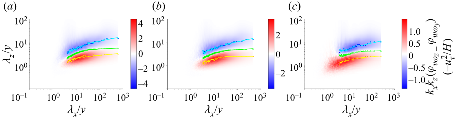
Figure 12. Ridges of spanwise wavelengths  $\lambda _z^u/y$ at minimum cospectrum (blue-filled cyan circles),
  $\lambda _z^d/y$ at maximum cospectrum (red-filled yellow squares) and
  $\lambda _z^*/y$ at zero cospectrum (green triangles), plotted log–log vs streamwise wavelength
  $\lambda _x/y$, together with the normalized 2-D cospectra
  $\varphi_{v\omega _z-w\omega _y}(k_x,k_z;y)$ for
  $y$ in the log layer. Power-law fits for the minimum, maximum and zero cospectral ridges at
  $\lambda _x \gtrsim 30y$, are given by cyan, yellow and green lines, respectively. Panels show: (a)
  $y^+=40$; (b)
  $y^+=53$; (c)
  $y^+=100$.
Table 2. Linear fits for  $(\lambda _x/y)\gtrsim 30$,
  $\lambda _z^u/y=a_u(\lambda _x/y)^{p_u}$,
  $\lambda _z^d/y=a_d(\lambda _x/y)^{p_d}$,
 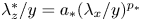 $\lambda _z^*/y=a_*(\lambda _x/y)^{p_*}$. Here,
  $a_u$,
  $a_d$ and
  $a_*$ are constants.

3.4. Coherent vortices and their vorticity flux contributions
There has long been interest in the role of coherent vortex structures in turbulent flows (Cantwell Reference Cantwell1981; Hussain Reference Hussain1986; Robinson Reference Robinson1991; Adrian Reference Adrian2007), with new insights related to exact Navier–Stokes solutions that represent such organized states (McKeon Reference McKeon2017; Graham & Floryan Reference Graham and Floryan2021). One of the drivers of this sustained attention is the empirical fact that coherent vortices contribute a disproportionate amount to turbulent transport, outsize relative to their small volume fraction in the flow. These considerations have motivated extensive efforts over many years to develop vortex identification methods, with classical methods discussed in prominent reviews (Chakraborty, Balachandar & Adrian Reference Chakraborty, Balachandar and Adrian2005; Kolář Reference Kolář2007) and with improved methods continuing to be developed (Haller et al. Reference Haller, Hadjighasem, Farazmand and Huhn2016) The bipartite character of the 2-D flux cospectrum discussed in the previous subsection provides the basis to investigate the coherent vortex structures which contribute separately to up-gradient and down-gradient vorticity transport. The straightforward idea is to decompose the flow at each  $y$-level into the contributions of two sets of eddies characterized by their support in the 2-D Fourier space
  $(k_x,k_z),$ with one field coming from eddies with negative (up-gradient) sign of the normalized flux cospectrum and the other from eddies with positive (down-gradient) sign. Methods of vortex visualization that have been applied to the full fields can then be applied to the two (nearly) orthogonal fields in order to identify the coherent vortices that contribute most significantly to up-gradient and down-gradient transport.
In supplementary materials, § F, we devise a convenient low-pass filter function  $\mathcal {D}(k_x,k_z,y)$ that selects the spectral region of up-gradient flux, while its complement high-pass function
  $\mathcal {D}^c(k_x,k_z,y)=1-\mathcal {D}(k_x,k_z,y)$ selects the region of down-gradient flux. The filter functions were chosen to be graded to avoid Gibbs-type oscillations in physical space due to sharp spectral cutoffs. The particular filter function
  $\mathcal {D}(k_x,k_z,y)$ that we employ is a Gaussian function with elliptical level sets and with rotation angle relative to the Cartesian axes that depend upon the wall distance
  $y.$ When extended to the space of signed wavenumbers by reflections in the Cartesian coordinate axes, the levels of this function (see figure F.13a) resemble the crossed wings of a dragonfly and hence we have dubbed this function the ‘dragonfly filter’. In the other panels of figure F.13 in the supplementary materials we illustrate how this filter selects regions of negative normalized flux cospectrum. All spatial fields
  $q(x,y,z)$ such as velocity and vorticity are then filtered by taking 2-D FFTs, multiplying by
  $\mathcal {D}(k_x,k_z,y)$ or
  $\mathcal {D}^c(k_x,k_z,y)$ and then taking a 2-D inverse FFT to obtain two fields, the contributions
  $q^U(x,y,z)$ of ‘U-type eddies’ and
  $q^D(x,y,z)$ of ‘D-type eddies’. We can then calculate separate nonlinear fluxes
 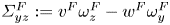 $\varSigma _{yz}^F:=v^{F}\omega _z^{F}-w^{F}\omega _y^{F}$ for both
  $F=U,D.$ Since off-diagonal terms such as
  $v^{U}\omega _z^{D}$ are small after averaging over both
  $x$ and
  $z,$ this yields a nearly additive decomposition for averages
 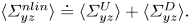 $\langle \varSigma _{yz}^{nlin}\rangle \doteq \langle \varSigma _{yz}^U\rangle +\langle \varSigma _{yz}^D\rangle.$
When can then visualize vortices for the two velocity fields  ${\boldsymbol {u}}^U$ and
  ${\boldsymbol {u}}^D.$ We present results here for the
  $\lambda _2$-criterion of Jeong & Hussain (Reference Jeong and Hussain1995) which is based on the intermediate eigenvalue
  $\lambda _2(\boldsymbol {\nabla }\boldsymbol {u})$ of the symmetric matrix
  $\boldsymbol {S}^2+\boldsymbol {\varOmega }^2$ where
  $\boldsymbol {S}$ and
  $\boldsymbol {\varOmega }$ are, respectively, the symmetric and anti-symmetric parts of
  $\boldsymbol {\nabla }\boldsymbol {u}.$ We can then define
  $\lambda _2^U:=\lambda _2(\boldsymbol {\nabla }\boldsymbol {u}^U)$ and
 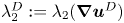 $\lambda _2^D:=\lambda _2(\boldsymbol {\nabla }\boldsymbol {u}^D)$ and visualize vortices by negative levels of these scalar fields. We have also considered other vortex visualization schemes such as the
  $Q$-criterion of Hunt, Wray & Moin (Reference Hunt, Wray and Moin1988) but, consistent with other works (Chakraborty et al. Reference Chakraborty, Balachandar and Adrian2005), we obtain very similar results from the different visualization criteria when applied to turbulent fields and we thus present here our results only for the
  $\lambda _2$-criterion. We follow the suggestion of Wu & Christensen (Reference Wu and Christensen2006) to visualize structures in inhomogeneous wall-bounded turbulence based on levels of the vortex discriminant function normalized by its variance, here
  $\lambda _2/\lambda _2^{rms}=-\beta.$ Since the vorticity magnitudes decrease rapidly with
  $y$, this normalization permits uniform visualization of coherent vortices at all wall distances. The imposed level is somewhat arbitrary but we choose here
  $\beta =1$ which is in the range of earlier related studies (Wu & Christensen Reference Wu and Christensen2006; Chen et al. Reference Chen, Adrian, Zhong, Li and Wang2014, Reference Chen, Li, Bai and Wang2018a,Reference Chen, Li, Bai and Wangb), which we discuss at length below.
We begin with a discussion of the coherent vortices for the high-pass field  ${\boldsymbol {u}}^D$, identified based on the discriminant function
  $\lambda _D.$ These structures are plotted in figure 13 and shall be referred to here as ‘
 $D$-type vortices’ since they arise from the field
  $\boldsymbol {u}^D$ which accounts for the down-gradient nonlinear vorticity flux away from the wall. We visualize here only the vortices in the log layer of the simulation, corresponding to
  $30< y^+<300.$ The vortex surfaces in the figure are coloured based on the pointwise values of the down-gradient flux
  $\varSigma _{yz}^D$ The most immediate observation about the
  $D$-type vortices is that they have a very similar morphology to the well-known ‘hairpin vortices’ that have been frequently visualized in the full velocity field
  ${\boldsymbol {u}}$ of turbulent wall-bounded flows, not only by the
  $\lambda _2$-criterion (Jeong et al. Reference Jeong, Hussain, Schoppa and Kim1997) but also by alternative methods such as swirling strength (Adrian & Liu Reference Adrian and Liu2002; Alfonsi et al. Reference Alfonsi, Ciliberti, Mancini and Primavera2011) and the
  $Q$-criterion (Wu & Moin Reference Wu and Moin2009). We note that most of these vortices are ‘prograde’ with
  $\omega _z<0$ and ‘retrograde’ vortices with
  $\omega _z>0$ are greatly outnumbered. Many of the hairpins also appear to be strongly asymmetric, with one much weaker leg, in agreement with some previous observations (Adrian Reference Adrian2007). Hairpin vortices or packets of hairpins are often considered to be plausible candidates for the ‘attached eddies’ in the AEM (Adrian Reference Adrian2007; Marusic & Monty Reference Marusic and Monty2019). Although we attempt here no detailed statistical analysis, the
  $D$-type vortices pictured in figure 13 appear indeed to be wall-attached structures, with feet of one or both legs planted in the near-wall region. These observations agree with the suggestion of Eyink (Reference Eyink2008) and others (Chen et al. Reference Chen, Adrian, Zhong, Li and Wang2014, Reference Chen, Li, Bai and Wang2018b) that the down-gradient transport of vorticity should be supplied by attached hairpin-type structures, although we recall the evidence from the previous subsection that D-type vortices are not self-similar at
  $Re_\tau =1000.$ An interesting fact that may be inferred from the colour plot in figure 13 is that
  $\varSigma _{yz}^D$ is not down-gradient (red colour) at every point on the
  $D$-vortices. In fact, there are points also of very large up-gradient transport (blue colour), which is permitted because the filter function
  $\mathcal {D}^c$ selects positive flux only in Fourier space not in physical space. We can see furthermore that the regions of the two different signs of transport are organized, with red (down-gradient) generally on the upstream side of the vortex and blue (up-gradient) generally on the downstream side. This tendency is even more obvious in an interactive 3-D version of figure 13 that can be found at https://www.cambridge.org/S0022112023006092/JFM-Notebooks/files/Figure-13/D-vortices.html made available in the JFM Notebook. This observation can be easily understood in terms of the direction of the Lamb vector calculated from the vorticity vector and the local vortex-induced velocity in the vicinity of a hairpin-type vortex.

Figure 13. Vortices identified using the  $\lambda _2$-criterion for the velocity field
  $\boldsymbol {u}^D$ filtered using
  $\mathcal {D}^c.$ Isosurfaces are plotted for
  $\lambda _2^D=-\lambda _2^{D,rms}$ and coloured by the nonlinear flux
  $\varSigma _{yz}^D$. The 3-D figure is available at https://www.cambridge.org/S0022112023006092/JFM-Notebooks/files/Figure-13/D-vortices.html. The data and code to generate such 3-D vortices are available at https://www.cambridge.org/S0022112023006092/JFM-Notebooks/files/Figure-13/D-vortices-plot.ipynb.
The net vorticity flux of all D-type eddies is indeed down-gradient, however, as illustrated by figure 14(a) which plots  $\langle \varSigma _{yz}^D\rangle$ normalized by
  $-u_\tau ^2/H$ vs
  $y.$ Not only is the normalized flux positive but in fact
  $\langle \varSigma _{yz}^D\rangle <-u_\tau ^2/H$ for all
  $y$ and it approaches almost
  $-7u_\tau ^2/H$ in the buffer layer. These large values are possible because they (plus the viscous flux) are nearly cancelled by the opposing up-gradient flux supplied by the complementary field
  ${\boldsymbol {u}}^U.$ In addition to the total
  $\langle \varSigma _{yz}^D\rangle,$ we can also calculate the partial average
  $\langle \varSigma _{yz}^D\rangle _\beta$ from the region of the vortex cores characterized by
  $\lambda _2^D<-\beta \lambda _2^{D,rms}.$ For
  $\beta =1$ this may be considered the direct contribution of the
  $D$-type vortices to the mean down-gradient flux. However, it is likely that this partial average on the cores underestimates the true contribution of the coherent vortices, which will also make an indirect contribution from a spatial neighbourhood influenced by induced motions from Biot–Savart (Wu & Christensen Reference Wu and Christensen2006; Chen et al. Reference Chen, Li, Bai and Wang2018b). As a crude estimate of this larger contribution from the region influenced by the coherent vortices, we consider the partial average
  $\langle \varSigma _{yz}^D\rangle _0$ over the region with
  $\lambda _2^D<0.$ Both of these partial averages are plotted also vs
  $y$ in figure 14(a). The fractional contributions of the vortex cores and the vortex neighbourhoods are furthermore plotted in figure 14(b). We can also calculate the area fractions of these two regions in the wall-parallel planes at each distance
  $y$ and these are plotted in figure 14(c). These plots show that the vortex cores contribute an increasing fraction of the down-gradient flux for increasing
  $y,$ starting from
  $\sim$5 % at
  $y^+=30,$ reaching
  $\sim$45 % at
  $y^+=150$, and remaining roughly constant then in the log layer, but vortex cores occupy only approximately
  ${\sim }7\,\%$ of the area at every wall distance. The flux fraction from the vortex-dominated region behaves similarly but is even larger, with
  ${\sim }30\,\%$ contribution at
  $y^+=30,$
  ${\sim }65\,\%$ at
  $y^+=150$ and remaining roughly constant thereafter, while occupying only approximately 40 % of the area. Thus, by either of the measures, the
  $D$-type vortices make a contribution to the down-gradient flux out of proportion to their volume in the flow.
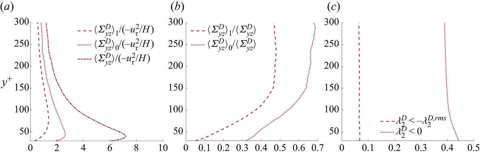
Figure 14. (a) Mean down-gradient vorticity flux and its contributions from  $D$-type coherent vortices,
  $\langle \varSigma _{yz}^D\rangle$. (b) Fractional contributions from
  $D$-type vortices,
  $\langle \varSigma _{yz}^D\rangle$. (c) Area fraction occupied by
  $D$-type vortices.
Our results closely mirror previous works which have studied the effects of coherent vortices on the transport of spanwise vorticity. Following the pioneering work of Wu & Christensen (Reference Wu and Christensen2006) on spanwise vortex contributions to Reynolds stress, Chen et al. (Reference Chen, Adrian, Zhong, Li and Wang2014) experimentally studied open channel flume flows at  $Re_\tau =382\sim 740$ using particle image velocimetry in 2-D vertical planes, which gave access to the velocities
  $u(x,y)$ and
  $v(x,y).$ Identifying coherent vortices by the swirling strength with
  $\beta =1.5$, they could then analyse their contribution to the advective flux
  $v\omega _z.$ They found many such coherent vortices with almost 97 % prograde at
  $y^+\simeq 50$ and this percentage declining with
  $y$ but still 65 % at
  $y^+=600,$ and it was conjectured that the prograde vortices were the heads of hairpin vortices. Chen et al. (Reference Chen, Adrian, Zhong, Li and Wang2014) observed as well a bipolar distribution of flux near the vortex cores, with
  $v'\omega _z'>0$ upstream and
  $v'\omega _z'<0$ downstream, which they explained also by local induced velocities. Finally, Chen et al. (Reference Chen, Adrian, Zhong, Li and Wang2014) found for the region
  $100< y^+<0.9 Re_\tau$ that coherent vortex cores contribute approximately 45 % to
  $\langle v\omega _z\rangle$ while occupying only 9 % of the area. All of these results for the total velocity field in 2-D planes are quite similar to ours for the high-pass filtered field component
  $\boldsymbol {u}^D$ in three dimensions.
The following paper of Chen et al. (Reference Chen, Li, Bai and Wang2018b) (see also Chen et al. Reference Chen, Li, Bai and Wang2018a) verified the results of Chen et al. (Reference Chen, Adrian, Zhong, Li and Wang2014), but in the channel-flow simulation of Del Alamo et al. (Reference Del Alamo, Jiménez, Zandonade and Moser2004) at  $Re_\tau =934.$ Because of the availability of full 3-D velocity fields, Chen et al. (Reference Chen, Li, Bai and Wang2018b) could apply the swirling strength criterion for various choices of
  $\beta$ in both 2-D planes and in three dimensions and they found that comparable results were obtained for both, although the 3-D criterion identified more coherent vortices than did the 2-D criterion. Chen et al. (Reference Chen, Li, Bai and Wang2018b) could also study the stretching flux
  $-w\omega _y$ and the full nonlinear flux
  $v\omega _z-w\omega _y$ and then investigate the coherent vortex contribution to each of these. In fact, Chen et al. (Reference Chen, Li, Bai and Wang2018b) decomposed the entire space domain into four exclusive point sets consisting of ‘filamentary vortices’ (FV), ‘non-filamentary vortices’ (NFV), ‘non-swirling vortex structures’ (NSVS) and ‘irrotational structures’, and all of these except the latter can contribute to vorticity flux. The FV structures correspond roughly to our vortex cores, but identified by swirling strength and a region growing algorithm, and the other structure types are precisely defined by Chen et al. (Reference Chen, Li, Bai and Wang2018a,Reference Chen, Li, Bai and Wangb). Thus, Chen et al. (Reference Chen, Li, Bai and Wang2018b) determined the fractional contributions of each of the first three types of structures (FV, NFV, NSVS) to the three fluxes (advective, stretching, total nonlinear) and they emphasized the dominant role of the FV structures. For the region
  $y^+>300$ of their simulation where
  $\langle w\omega _y\rangle >0$ (down-gradient), FV structures contribute more than 80 % while occupying only 15 % of the volume. Likewise, for the region
  $y^+>50$ where
  $\langle v\omega _z-w\omega _y\rangle <0$ (down-gradient), FV structures contribute more than 60 % while occupying area less than 15 %. They concluded that: ‘Compared with the other three structures, FV play a very important role in velocity–vorticity correlations and the net force’.
From our perspective, however, a very important result of Chen et al. (Reference Chen, Li, Bai and Wang2018b) that was never explicitly mentioned by them is the fact that the FV contributions to all three of the fluxes are negative (down-gradient) everywhere, that is,  $\langle v\omega _z\rangle _{FV}<0$,
  $-\langle w \omega _z\rangle _{FV} <0$ and
  $\langle v\omega _z- w \omega _z\rangle _{FV} <0$ for all
  $y$. These signs can be inferred from the data plotted in figures 2(b) and 9 of Chen et al. (Reference Chen, Li, Bai and Wang2018b). Since, however,
  $-\langle w\omega _y\rangle >0$ for
  $y^+<300$ and
  $\langle v\omega _z-w\omega _y\rangle >0$ for
  $y^+<50$ in the simulation studied by Chen et al. (Reference Chen, Li, Bai and Wang2018b), this means that the FV structures are not only not dominant in these regions but in fact give a contribution of the wrong sign! See figure 9(c–d) in Chen et al. (Reference Chen, Li, Bai and Wang2018b). Put another way, the FV structures do not account for the up-gradient vorticity transport in these regions. This is understandable if one can essentially identify the FV structures of Chen et al. (Reference Chen, Li, Bai and Wang2018b) with our
  $D$-type vortices, which contribute always a net down-gradient flux. This identification is plausible based on the evidence of visualizations, since the
  $D$-type vortices shown in our figure 13 resemble quite closely the vortex structures detected by the swirling strength criterion in the full velocity field (Adrian & Liu Reference Adrian and Liu2002; Alfonsi et al. Reference Alfonsi, Ciliberti, Mancini and Primavera2011). In any case, the important result of Chen et al. (Reference Chen, Li, Bai and Wang2018b) not emphasized by them is that it is the NFV and NSVS structures which account for the up-gradient vorticity transport observed closer to the wall. Unfortunately, the works of Chen et al. (Reference Chen, Li, Bai and Wang2018a,Reference Chen, Li, Bai and Wangb) did not attempt to visualize the NFV and NSVS structures or to clarify their morphology and dynamics.
We can now illuminate the nature of such structures by vortex visualizations for the low-pass field  $\boldsymbol {u}^U$, using the discriminant function
  $\lambda _2^U$ and
  $\beta =1.$ These structures are plotted in figure 15 and shall be referred to here as ‘
 $U$-type vortices’ since they arise from the field
  $\boldsymbol {u}^U$ which accounts for the up-gradient nonlinear vorticity flux toward the wall. As before, we visualize only the vortices in the log layer of our simulation and the vortex surfaces are coloured based on the values of the up-gradient flux
  $\varSigma _{yz}^U.$ The
  $U$-type vortices visualized in figure 15 have a pancake structure, vertically flattened and elongated along the streamwise direction but especially along the spanwise direction. Their characteristic shape becomes even clearer in the interactive 3-D version of figure 15 available at https://www.cambridge.org/S0022112023006092/JFM-Notebooks/files/Figure-15/U-vortices.html. These are exactly the type of vortex structures one would imagine to arise from the Lighthill (Reference Lighthill1963) mechanism of correlated downflow and lateral stretching. In fact, the roughly twice longer extents spanwise than streamwise correspond well to Lighthill's remark that ‘some longitudinal deformation is usually also present, which reduces the need for lateral deformation (perhaps, on average, by half)’. Note, that these structures, ultimately based on the 2-D cospectra plotted in figure 11, can be interpreted as evidence for a cascade process similar to that for momentum, since the vorticity transfer in space is observed to be carried by a hierarchy of eddies whose size depends upon wall distance. However, there is no obvious self-similarity of these structures in scale and, according to the results presented in our figure 8 and table 2, one might expect the ratio
  $\lambda _x/\lambda _z$ to increase with scale. The
  $U$-type vortices show also no obvious attachment to the wall, being mainly horizontal to it. Indeed, an extension of the AEM by Perry & Marusic (Reference Perry and Marusic1995) and Marusic & Perry (Reference Marusic and Perry1995) introduced in addition to the ‘type-A’ attached eddies also ‘type-B’ eddies to represent the wake flow in the outer layer and small-scale ‘type-C’ eddies to represent the Kolmogorov range. The type-B eddies were viewed as detached vortex tubes which undulate in the spanwise direction, thus somewhat resembling our
  $U$-type eddies (see figure 3 of Perry & Marusic Reference Perry and Marusic1995). More recently, Hu, Yang & Zheng (Reference Hu, Yang and Zheng2020) have attempted to decompose turbulent channel-flow fields at
  $Re_\tau =5200$ into small-scale eddies, attached eddies, and detached eddies, and their
  $|u|$-isosurfaces for the detached eddies (see their figure 19d) have a similar pancake structure as our
  $U$-type vortices. We have also checked that the vorticity in the
  $U$-type vortices is predominantly spanwise and prograde consistent with lateral stretching of pre-existing vorticity. This is demonstrated by figure G.14 in the supplementary materials, where we colour these vortices by the cosine of the angle made by the vorticity vector
  $\boldsymbol {\omega }^U$ with the
  $z$-axis and find the prevalence of values close to
  $-1$, denoting prograde spanwise aligned vortices. Finally, we observe flux bipolarity of the
  $U$-type vortices just as for the
  $D$-type, with red (down-gradient) generally on the upstream side of the vortex and blue (up-gradient) generally on the downstream side. This tendency is again more obvious in a 3-D version of the figure available in the JFM Notebook.
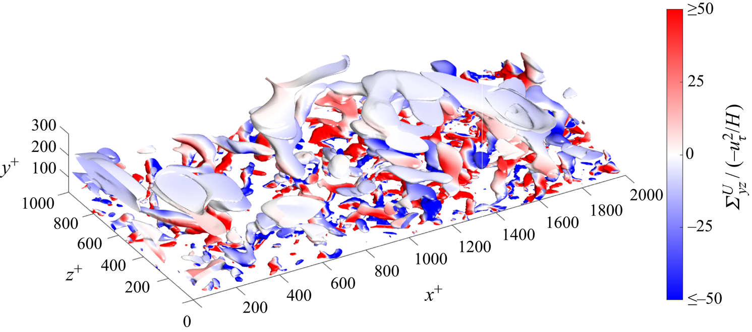
Figure 15. Vortices identified using the  $\lambda _2$-criterion for the velocity field
  ${\boldsymbol {u}}^U$ filtered using
  $\mathcal {D}.$ Isosurfaces are plotted for
  $\lambda _2^U=-\lambda _2^{U,rms}$ and coloured by the nonlinear flux
  $\varSigma _{yz}^U$. The 3-D figure is available at https://www.cambridge.org/S0022112023006092/JFM-Notebooks/files/Figure-15/U-vortices.html. The data and code to generate 3-D vortices are available at https://www.cambridge.org/S0022112023006092/JFM-Notebooks/files/Figure-15/U-vortices-plot.ipynb.
Despite large contributions to the vorticity flux of both signs, however, the net flux supplied by all  $U$-type eddies is up-gradient. This is verified by the data in figure 16(a), which plots
  $\langle \varSigma _{yz}^U\rangle$ normalized by
  $-u_\tau ^2/H$ vs
  $y.$ Similar to the result for the
  $D$-type vortices,
 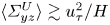 $\langle \varSigma _{yz}^U\rangle \gtrsim u_\tau ^2/H$ across most of the log layer and approaches
  $10 u_\tau ^2/H$ at the lower
  $y$ range where it must cancel most of the down-gradient flux from the
  $D$-type eddies and viscous diffusion. For the largest
  $y^+\sim 300$ in the log layer,
 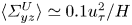 $\langle \varSigma _{yz}^U\rangle \simeq 0.1 u_\tau ^2/H$ and still cancels part of the contribution from the
  $D$-type eddies. In addition to the total
  $\langle \varSigma _{yz}^U\rangle,$ we can also calculate the partial averages
  $\langle \varSigma _{yz}^U\rangle _\beta$ for the condition
 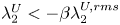 $\lambda _2^U<-\beta \lambda _2^{U,rms}$ with
  $\beta =1$ (vortex cores) and
  $\beta =0$ (vortex neighbourhoods). Both of these partial averages are plotted also vs
  $y$ in figure 16(a), the fractional contributions of the vortex cores and the vortex neighbourhoods are plotted in figure 16(b), and the corresponding area fractions plotted in figure 16(c). We observe that the cores of the
  $U$-type vortices account for
  $\sim$20 %–30 % of the up-gradient flux but occupy only approximately 10 % of the area, while regions dominated by the
  $U$-type vortices provide
  $\sim$60 %–70 % of the flux but occupy only approximately 45 % of the area. The coherent
  $U$-type vortices thus contribute a percentage of the up-gradient flux roughly twice their area in the flow. This is not as outsize as the contribution of the
  $D$-type vortices to the down-gradient flux and the lower performance may be due to our rote application of the
  $\lambda _2$-criterion for vortex identification in
  $\boldsymbol {u}^U.$ This criterion was designed by Jeong & Hussain (Reference Jeong and Hussain1995) to detect rapidly swirling vortex tubes with low-pressure cores, whereas the
  $U$-type vortices clearly have a distinct structure. It is also possible that our filter function
  $\mathcal {D}$ does not have spectral support optimally chosen. More appropriate filter kernels and discriminant functions can probably be devised to characterize better the coherent
  $U$-type vortices that contribute most to the up-gradient vorticity transport.

Figure 16. (a) Mean down-gradient vorticity flux and its contributions from  $U$-type coherent vortices,
  $\langle \varSigma _{yz}^U\rangle$. (b) Fractional contributions from
  $U$-type vortices,
  $\langle \varSigma _{yz}^U\rangle$. (c) Area fraction occupied by
  $U$-type vortices.
4. Discussion and conclusions
The main objective of this work has been to elucidate the dynamics involved in turbulent transport of spanwise vorticity normal to a solid wall, motivated by the direct connection of this ‘vorticity cascade’ to turbulent drag. We have carried out a numerical study for a canonical case of pressure-driven Poiseuille flow in a channel with plane-parallel walls. We find that the mean vorticity transfer is the result of two intensely competing processes: an up-gradient transfer that concentrates spanwise vorticity strongly near the wall and a slightly greater down-gradient transfer that disposes of the fresh spanwise vorticity generated at the wall by the mean pressure gradient. This is exactly the picture suggested by Lighthill (Reference Lighthill1963), who proposed also a concrete mechanism for up-gradient transport by inflow to the wall correlated with lateral stretching of vortex lines and outflow correlated with lateral relaxation. We have presented here detailed evidence for the validity of Lighthill's mechanism in the case of turbulent channel flow based upon: (i) correlations of wall-normal velocity with flux of spanwise vorticity, (ii) velocity–vorticity cospectra that identify the eddies involved in nonlinear vorticity transport in the two directions and (iii) visualization of the coherent vortex structures which contribute dominantly to the transport. All of the observations that we have accumulated are consistent with the proposed mechanism. In addition, we have provided evidence to support the interpretation of this vorticity flux as a cascade similar to momentum cascade, in that the spatial transport of vorticity is associated also with a stepwise transfer in scale. This verification has consequences that extend far beyond channel flow, because Lighthill (Reference Lighthill1963) suggested that the up-gradient transfer mechanism has very general validity for all turbulent flows interacting with solid walls, e.g. high Reynolds number flows around bluff bodies or airplane wings. In fact, Lighthill (Reference Lighthill1963) proposed this mechanism to explain why turbulent boundary layers with concentrated vorticity form generally near solid walls. This is the necessary prelude to another fundamental vortex interaction with solid walls, the violent eruption of vorticity away from the wall (Smith et al. Reference Smith, Walker, Haidari and Sobrun1991; Doligalski, Smith & Walker Reference Doligalski, Smith and Walker1994; Lenaers et al. Reference Lenaers, Li, Brethouwer, Schlatter and Örlü2012), which apparently underlies phenomena such as boundary-layer separation behind bluff bodies and frequent ejections from the walls in turbulent flows over flat plates and in straight pipes.
Our work exposes also a limitation of the ‘attached eddy model’ of Townsend (Reference Townsend1976) because we find considerable evidence that down-gradient vorticity flux out from solid walls is provided indeed by attached eddies but that the competing up-gradient flux into the walls is carried by detached eddies. Of course, many extensions of the AEM have been proposed previously. We have already mentioned the early work of Perry & Marusic (Reference Perry and Marusic1995), Marusic & Perry (Reference Marusic and Perry1995) and see also more recent papers of Chandran et al. (Reference Chandran, Monty and Marusic2020) and Hu et al. (Reference Hu, Yang and Zheng2020). The spectral aspects of the extension by Perry & Marusic (Reference Perry and Marusic1995) and Marusic & Perry (Reference Marusic and Perry1995) focus on the streamwise spectrum  $\phi _{uu}(k_x)$, as summarized in figure 16 of Marusic & Perry (Reference Marusic and Perry1995), reproduced in figure 11 of Marusic & Monty (Reference Marusic and Monty2019). Our present cospectral results echo features of this model upon suitable interpretation. The model of Perry & Marusic (Reference Perry and Marusic1995) and Marusic & Perry (Reference Marusic and Perry1995) has an overlap in the streamwise scales of type-A and type-B eddies, with the latter contribution dominating at larger streamwise scales. This type of behaviour is seen also in our 2-D flux cospectra in the log layer, plotted in figures 11(d)–11(f), where the
  $U$-type eddies dominate at large streamwise scales but overlap with the support of the
  $D$-type eddies at smaller streamwise scales. Note, however, that the effect of Type-B eddies in the AEM extension of Perry & Marusic are supposed to diminish upon approaching the wall, whereas the vorticity transport effects of the
  $U$-type eddies in our work increase and dominate close to the wall. Unlike previous proposals to extend the AEM, our work has revealed that detached eddies play a fundamental dynamical role in the near-wall region, with direct importance to drag generation and reduction. The closest connection of our results are with those of Chen et al. (Reference Chen, Li, Bai and Wang2018b), who found that NFV and NSVS rather than FV are responsible for the dominant up-gradient nonlinear vorticity transport near the wall.
In this paper we have exploited a database of a turbulent channel flow at  $Re_\tau =1000$ and we have compared with related experiments and simulations at comparable Reynolds numbers. However, empirical data are available at a broader range of Reynolds numbers, both lower Reynolds number simulation data (Bernard Reference Bernard1990; Crawford & Karniadakis Reference Crawford and Karniadakis1997) and field experiments at much higher Reynolds numbers (Priyadarshana et al. Reference Priyadarshana, Klewicki, Treat and Foss2007; Morrill-Winter & Klewicki Reference Morrill-Winter and Klewicki2013). We do not expect the main conclusions of our work to be
  $Re$-dependent and we are aware of no data available at other Reynolds numbers which contradicts them. However, some details of the story we have presented may change with
  $Re.$ For example, it is well known that many predictions of the AEM are observable only for
  $Re\gg 1$ and, in particular, Chandran et al. (Reference Chandran, Baidya, Monty and Marusic2017) estimate that the similarity relation
  $\lambda _z\sim \lambda _x$ for attached eddies and clear
  $k^{-1}$ energy spectra for both
  $k_x$ and
  $k_z$ should be observable only for
  $Re_\tau >60\,000.$ Thus, our conclusion in § 3.3 that
  $D$-type and
  $U$-type eddies are non-self-similar might be Reynolds-number dependent, especially since self-similarity for 2-D energy cospectra that is expected from attached eddies is not observed either at comparable
  $Re_\tau$ (Del Alamo et al. Reference Del Alamo, Jiménez, Zandonade and Moser2004; Chandran et al. Reference Chandran, Baidya, Monty and Marusic2017). Thus, extending our analysis to higher Reynolds numbers is an important direction for future research.
Another important direction is the investigation of turbulent vorticity dynamics by means of stochastic Lagrangian methods (Constantin & Iyer Reference Constantin and Iyer2011; Eyink et al. Reference Eyink, Gupta and Zaki2020a). The heuristic arguments of Lighthill (Reference Lighthill1963) are essentially Lagrangian and invoke the remarkable ‘frozen-in’ properties enjoyed by vortex lines in smooth ideal Euler flows. In a physical turbulent flow, however, these familiar properties of ideal vortex-lines suffer fundamental modifications by viscous diffusion, which can be exactly captured by the stochastic Lagrangian representation of the vortex dynamics. These methods have already proved powerful to verify the validity of Lighthill's argument for origin of large magnitudes of wall vorticity in a transitional zero-pressure-gradient boundary layer (Wang et al. Reference Wang, Eyink and Zaki2022). The advantage of these methods compared with the Eulerian analysis in the present work is that they provide a complete and unambiguous account of the origin of the vorticity at any point in the flow, with precise and quantitative information about the physical mechanisms involved. Such stochastic Lagrangian methods have already been applied to ‘ejections’ and ‘sweeps’ in the buffer layer of the same  $Re_\tau =1000$ turbulent channel flow studied in this paper, where it was demonstrated that the spanwise vorticity in those events is not assembled abruptly from wall vorticity but instead over many hundreds of viscous times (Eyink, Gupta & Zaki Reference Eyink, Gupta and Zaki2020b). It would be very illuminating to apply these methods in the log layer of the channel flow, reconstructing the spanwise vorticity under conditions of inflow and outflow and determining its origin unambiguously. The existing numerical schemes for the stochastic Lagrangian approach are quite inefficient in the log layer, however, because the Monte Carlo sampling errors grow exponentially in time. New algorithmic approaches are probably therefore required.
Finally, the insights that we have obtained in this work about the Eulerian vorticity dynamics described by the Huggins vorticity flux tensor (1.4) can be exploited to understand drag generation and reduction via the detailed Josephson–Anderson (JA) relation (Huggins Reference Huggins1970, Reference Huggins1994; Eyink Reference Eyink2008, Reference Eyink2021). Such work is already in progress (Kumar & Eyink, unpublished). We have thus intentionally omitted in the present paper any discussion of the work of Yoon et al. (Reference Yoon, Ahn, Hwang and Sung2016) which directly relates velocity–vorticity correlations to mean drag by a version of the identity of Fukagata, Iwamoto & Kasagi (Reference Fukagata, Iwamoto and Kasagi2002). This discussion requires a careful comparison with the JA-relation, which will be done in future work by Kumar & Eyink. The connections between these two approaches is indeed not straightforward, e.g. down-gradient nonlinear vorticity flux produces drag in the JA-relation but reduces drag in the identity of Yoon et al. (Reference Yoon, Ahn, Hwang and Sung2016)! Here, we just mention the principal difference that, whereas the identity of Yoon et al. (Reference Yoon, Ahn, Hwang and Sung2016) represents the mean drag in a Reynolds averaging approach, the JA-relation connects the drag instantaneously in time to the vorticity flux throughout the flow volume. The shift away from ensemble flow statistics to recognize the dynamical heterogeneity and intermittency of drag has proved important, for example, in the problem of polymer drag reduction (Xi Reference Xi2019). Our results here shed new light on the latter problem, because they imply that drag can be reduced instantaneously either by decreasing the down-gradient flux of spanwise vorticity or by increasing the up-gradient flux, or both. This will also be the subject of future work.
Supplementary material
Supplementary material and Computational Notebook files are available at https://doi.org/10.1017/jfm.2023.609. Computational Notebooks can also be found online at https://www.cambridge.org/S0022112023006092/JFM-Notebooks.
Acknowledgements
We thank Professors N. Goldenfeld, B. Hof, Y. Pomeau and T. Zaki for fruitful discussions and the JHTDB team for their help and support of the public numerical turbulence laboratory.
Funding
We thank also the Simons Foundation for support of this work through the Targeted Grant No. MPS-663054, ‘Revisiting the Turbulence Problem Using Statistical Mechanics’, and the National Science Foundation (Grant No. CSSI-210387) for support of JHTDB and of pursuing analysis of wall-bounded turbulence.
Declaration of interests
The authors report no conflict of interest.


 Open access