


Introduction
Glacier changes are considered the best natural indicators of climatic change (Reference Lemke and SolomonLemke and others, 2007) because they visualize small changes in climatic parameters with pronounced geometric changes; for example, a 0.1°C temperature increase per decade can result in length changes of several hundred meters (Oerlemans, 2005). The measurement of glacier-length changes is thus an important task in global climate-related monitoring programmes Global Terrestrial Observing System (GTOS)/Global climate observing System (GCOS) and is integrated in the tiered system of the Global Terrestrial Network for Glaciers (GTN-G) at the tier 4 level. As the sampling of measurements is often sparse in remote regions, repeated glacier inventories (tier 5) should assess the overall changes of the complete sample after a few decades, a typical response time for most mountain glaciers (Reference Haeberli, Bamber and PayneHaeberli, 2004). In many parts of the world, a first glacier inventory has been compiled from aerial photography dating from the 1960s and 1970s, and the results published in the World Glacier Inventory (WGI; Reference Haeberli, Bösch, Scherler, Østrem and WallénWGMS, 1989). After 30–40 years of pronounced glacier changes, a new inventory is overdue in many countries. Today, multispectral satellite data at 10–30 m spatial resolution (e.g. Landsat Thematic Mapper (TM)/Enhanced Thematic Mapper Plus (/ETM+), Terra Advanced Spaceborne Thermal Emission and Reflection Radiometer (ASTER), SPOT High Resolution Visible (HRV) facilitates glacier mapping over large and remote areas (Reference Paul and KääbPaul and Kääb, 2005), and automated mapping methods can be applied to several sensors (Reference Paul, Kääb, Maisch, Kellenberger and HaeberliPaul and others, 2002; Reference RaupRaup and others, 2007).
Many studies have already calculated changes between a former and a more recent satellite-derived dataset, with most of them indicating strong or even accelerated glacier decline in the past few decades (e.g. Reference Khromova, Dyurgerov and BarryKhromova and others, 2003; Reference Paul, Kääb, Maisch, Kellenberger and HaeberliPaul and others, 2004; Reference Silverio and JaquetSilverio and Jaquet, 2005; Reference Li, Zhu, Zhang, Pei, Qin and ZhouLi and others, 2006). A systematic approach comprising space-borne glacier mapping is followed by the Global Land Ice Measurements from Space (GLIMS) initiative, which, among its other goals, aims to provide digital glacier outlines for all the glaciers of the world, thus complementing the WGI and establishing a basic dataset for further comparison and change assessment (Reference KargelKargel and others, 2005; further information about GLIMS can be found at http://glims.org). Such digital glacier outlines are mandatory for the correct calculation of changes because it is often very unclear to which glaciers point information stored in the WGI refers.
In Norway, the most recent glacier inventories were compiled in the early 1970s for northern Scandinavia (Reference Østrem, Haakensen and MelanderØstrem and others, 1973) and in the 1980s for southern Norway (Reference Østrem, Selvig and TandbergØstrem and others, 1988). The inventory for northern Scandinavia (including glaciers in Sweden) is based on maps and aerial photographs from the 1950s and 1960s, and is referred to as Atlas73 hereafter. For the regions analysed here, the aerial photographs are from 1968 (Svartisen) and 1961 (Blåmannsisen). According to the length-change measurements in Norway, some glaciers have retreated whereas others have advanced over the past few decades, with a pronounced regional variability (Reference Andreassen, Kjøllmoen, Knudsen, Whalley and FjellangerAndreassen and others, 2000, Reference Andreassen, Elverøy, Kjøllmoen, Engeset and Haakensen2005). As a consequence, the current overall state of the glaciers is not well known. As glacier melt is an important source of water for hydropower generation in Norway, an assessment is desirable. Hence, the Norwegian Water Resources and Energy Directorate (NVE) decided to create a new glacier inventory from satellite data within the framework of the GLIMS initiative.
A pilot study for the new Norwegian inventory focused on the Jotunheimen region and the accuracy of the applied glacier mapping (Reference Andreassen, Paul, Kääb and HausbergAndreassen and others, 2008). We here present the results for the Svartisen region, with a special focus on methodological challenges. The objectives of this study are: (1) presentation of basic glacier inventory data for the Svartisen region; (2) assessment of glacier changes since the first glacier inventory; and (3) a discussion of the methodological challenges related to snow conditions, location of drainage divides and comparison of glacier inventories.
Study Site and Input Data
Description of the study site
The study site is prescribed by the perimeter of the Landsat ETM+ scene 199–13 (path–row) and covers approximately the region, 65.9–68.0° N, 11.1–16.7° E (Fig. 1). Apart from some cirrus clouds in the north (which allow glacier mapping underneath) and some optically thick cumulus clouds in the east, the scene is cloud-free. It covers three larger ice masses: (1) Vestisen ice cap (∼218 km2; 30–1580 m a.s.l.), the source of several outlet glaciers, including the well-studied outlet Glacier Engabreen (e.g. Reference Geist, Elvehøy, Jackson and StötterGeist and others, 2005; Reference Jackson, Brown and ElvehøyJackson and others, 2005; Reference SchulerSchuler and others, 2005); (2) Østisen (∼149 km2; 200–1590 m a.s.l.), which is composed of an ice cap with outlet glaciers and one separated valley glacier with a large accumulation area (Austerdalsisen); and (3) Blåmannsisen ice cap (86 km2; 820–1530 m a.s.l.) with several outlet glaciers dominating the northeastern part of the test site (Fig. 1). Some smaller valley and several mountain and cirque glaciers are situated along two ridges with a northeastern orientation to the north of Østisen. Perennial snow banks and firn fields, as well as several ice aprons, are found in many places within the scene, causing some problems in glacier identification. Abundant lakes (small to large in size and of variable turbidity), oriented scars from the last ice age and several fjords form a large part of the landscape (Fig. 1). A few glaciers are currently in contact with lakes that are partly used for hydropower purposes.
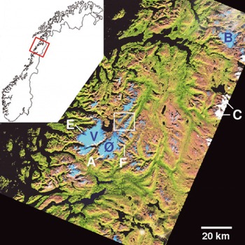
Fig. 1. Overview of the test site with an ETM+ band 5, 4, 3 (as red, green, blue) false-colour composite showing glacierized areas in light blue (see inset map for location in Norway). Letters denote: A, Austerdalsisen; B, Blåmannsisen; C, clouds; E, Engabreen; F, Fingerbreen; Ø, Østisen; V, Vestisen. The white square denotes the subregion of Figure 5. Figure 6 is located south of this region.
There is a strong precipitation gradient from west to east in Norway, which governs the degree of glacierization to some extent (Reference Østrem, Selvig and TandbergØstrem and others, 1988). At present, seasonal mass-balance and length-change measurements in the study region are performed only at Engabreen (Reference KjøllmoenKjøllmoen and others, 2007; Reference Elvehøy, Jackson and AndreassenElvehøy and others, 2009). However, shorter periods of measurement are available from several other glaciers (Reference Andreassen, Elverøy, Kjøllmoen, Engeset and HaakensenAndreassen and others, 2005; Reference KjøllmoenKjøllmoen and others, 2007). These reveal a strong regional and temporal variability of mass balance and length over the past three decades. Whereas some glaciers have exhibited positive mass balance and terminus advance (e.g. Engabreen), others in the same period lost mass and retreated (Reference Andreassen, Kjøllmoen, Knudsen, Whalley and FjellangerAndreassen and others, 2000, Reference Andreassen, Elvehøy and Kjøllmoen2002).
A rough climatic classification of the glaciers in the region can be derived from the mean annual air temperature (MAAT) at the steady-state equilibrium-line altitude (ELA0). For Engabreen, the ELA0 is at 1170 m (Reference Haeberli, Hoelzle and ZempWGMS, 2007) and the MAAT in the period 1961–90 at the weather station Glomfjord (40 m a.s.l., located about 17 km to the north of Engabreen) is about 5°C (http://met.no). This gives about −2°C at the ELA0 of Engabreen using a standard atmospheric lapse rate (0.65°C (100 m)−1), implying that most glaciers in this region are temperate. The Svartisen region was, and still is, the target of several glaciological studies, a few of which have been mentioned above. With respect to glacier mapping, one of the most recent and comprehensive studies was performed within the Operational Monitoring of European Glacial Areas (OMEGA) project, which investigated a large variety of technologies to study glacier changes (http://omega.utu.fi) and had one focus on Engabreen.
Applied input datasets
The Landsat ETM+ scene from 7 September 1999 (also available from the Global Land Cover Facility, GLCF) was provided in an orthorectified version (UTM projection, zone 33, WGS84 datum) by the Norsk Satelittdataarkiv (Norwegian Archive of Satellite Data). The geometric accuracy was tested with a set of 13 manually selected control points (CPs) that were approximately evenly distributed over the scene and revealed an accuracy of 0.5 pixels (15 m). The digital overlay with independently digitized vector datasets also shows a good match (Fig. 2).

Fig. 2. Mapping accuracy and drainage divides for Blåmannsisen ice cap, with various vector datasets shown as an overlay: glacier outlines with ETM+ in 1999 (red) and from Statens Kartverk in 1985 (white), 50 m elevation contours (grey), glacier labels from the WGI (black dots), approximate drainage divides from Atlas73 (black), original hydrologic units based on the bedrock topography (blue), and adjusted drainage divides based on a flow-direction grid from a DEM (yellow). Image size is 15.3 km × 14.0 km. The scale bar is 1 km.
Digital glacier outlines based on the national topographic map series at scale 1 :50 000 (hereafter called N50) from Statens Kartverk (the Norwegian mapping authorities) were used for comparison and change assessment with the Landsat-derived dataset. In the southern part of the scene, the glacier outlines on these maps were made from the same aerial photography, taken in 1968, that was used for Atlas73, but the interpretation by Statens Kartverk consists of a higher number of glacier polygons and also includes perennial snowfields. In the northern part of the scene (Blåmannsisen) the outlines are based on 1985 aerial photography (personal communication from J.H. Tallhaug, Statens Kartverk, 2008). In some parts of Vestisen and Østisen, the N50 glacier outlines of the study region had been updated with more recent surveys from the 1990s. Compared with an independently digitized vector dataset that refers to the 1968 extent, some glaciers had clearly changed size. To be consistent for the change assessment, we have replaced the updated outlines from the 1990s with the 1968 extent in these regions. Standard empirical rules used in photogrammetry and mapping result in an estimated horizontal rootmean-square error (RMSE) for the outlines in the order of 5–10 m, not taking into account any interpretation uncertainty during the compilation process.
A digital elevation model (DEM) with 25 m cell size was obtained from Statens Kartverk and has been used to calculate topographic glacier parameters such as highest, lowest and mean elevation, or mean slope and aspect of each glacier (see below). The DEM has a RMSE of 4–6 m (personal communication from J.H. Tallhaug, 2008). It must be noted that the DEM was derived from the N50 maps, which were mostly obtained in 1968 but included partial updates in 1993 (southern part of the scene) and 1985 (northern part), as described above. This mostly influences the accuracy of the calculated lowest elevation, as a retreated terminus could be located now at the elevation of the former DEM surface instead of at the ground. The related overestimation could be in the range 10–50 m and must be corrected when a higher accuracy for this parameter is required. The DEM from the Shuttle Radar Topography Mission (SRTM) acquired in February 2000 would fit better to the Landsat dataset, but our test site is located north of the Arctic Circle and is thus not covered by the SRTM DEM.
The hydrologic basins (called ‘Regine’ in Norway) are available in a digital vector format and were provided by NVE. They were originally produced by NVE, mostly by hand digitization of the N50 map sheets. For Vestisen, Østisen and Blåmannsisen, they are also based on hydrologic units resulting from extrapolated glacier beds (Reference SætrangSætrang, 1988; Reference KennettKennett, 1990; Reference Kennett, Rolstad, Elvehøy and RuudKennett and others, 1997). Unfortunately, many of the ice divides, as used in Atlas73 (Reference Østrem, Haakensen and MelanderØstrem and others, 1973), disagreed with the Regine basins, and an attempt at free-hand digitization of the former drainage divides (i.e. without scanning and proper geolocation of the original maps) revealed differences too large compared to the glacier areas as reported in Atlas73 (Fig. 2). However, the printed overview maps in Atlas73 are used to guide glacier identification. For the new inventory, which has been transferred to the GLIMS database, the Regine from NVE with some additional editing are used.
Glacier coordinates from the WGI were transformed to a point data layer in UTM33 projection that was later intersected with the basin layer to allow the selection of glaciers in a geographic information system (GIS). As the dataset had a sufficient number of digits (three) behind the dot, they were in a neighbourhood approximately 100 m from the glacier centre (Fig. 2); a few of the points had to be shifted to a new location because their previous position had been outside the corresponding glacier basin. Most of the data processing for this study (glacier mapping, editing, data retrieval) was performed within the GIS ArcInfo 9.0 (ESRI, 2004) using the Grid, ArcEdit and Tables modules.
Data Processing
Technical issues
Techniques for automated glacier mapping from multispectral satellite data have been tested thoroughly in the literature (e.g. Reference Sidjak and WheateSidjak and Wheate, 1999; Reference AlbertAlbert, 2002; Reference PaulPaul, 2002; Reference Paul, Kääb, Maisch, Kellenberger and HaeberliPaul and others, 2002; Reference Paul and KääbPaul and Kääb, 2005; Reference RaupRaup and others, 2007). The most efficient method is based on a thresholded ratio image from the raw digital numbers (DN) of bands TM3 or TM4 and TM5 that utilizes the spectral differences of ice and snow in the shortwave infrared part of the spectrum compared with other surfaces. The method is simple to apply, the threshold value is robust and the results are very accurate for debris-free ice (Reference AlbertAlbert, 2002; Reference Paul, Huggel, Kääb, Kellenberger and MaischPaul and others, 2003; Reference Andreassen, Paul, Kääb and HausbergAndreassen and others, 2008). Other methods, such as the normalized difference snow index (NDSI), have also been used in automated glacier mapping (e.g. Reference Racoviteanu, Arnaud, Williams and OrdoñezRacoviteanu and others, 2008a) and yield nearly identical results (Reference Paul and KääbPaul and Kääb, 2005). As the spectral range of TM5 (1.55–1.75 μm) is also covered by several other sensors (e.g. ASTER, SPOT, ETM+, Indian Remote-sensing Satellite (IRS), moderate-resolution imaging spectroradiometer (MODIS)), both methods are widely applicable (Reference KääbKääb and others, 2003; Reference Racoviteanu, Williams and BarryRacoviteanu and others, 2008b). The GIS-based processing of the classified glacier map (e.g. used for raster–vector conversion and digitizing/intersection with drainage divides) also allows fast and automated calculation of topographic glacier parameters by fusion of the glacier outlines with a DEM or products thereof (Reference Paul, Kääb, Maisch, Kellenberger and HaeberliKääb and others, 2002; Reference Khalsa, Dyurgerov, Khromova, Raup and BarryKhalsa and others, 2004; Reference PaulPaul, 2007).
In this study, a thresholded ratio image where pixels are classified as ice or snow when (TM3/TM5) > 2.6 is used. An additional threshold in TM1 (DNs >59) was applied to improve glacier mapping in cast shadow (Reference Paul and KääbPaul and Kääb, 2005). Both thresholds were selected interactively in the most sensitive region (shadow) to minimize the workload for post-processing (e.g. Reference RaupRaup and others, 2007). In Figure 2 the results of the automated method are illustrated for Blåmannsisen ice cap, where, even under difficult mapping conditions (underneath thin cirrus clouds and with bare ice in cast shadow), glacier boundaries are mapped well. Whereas few glacier outlines were corrected for debris cover, a larger effort was required to correct wrongly classified lakes. Although automated methods for lake detection from multispectral data exist (e.g. Reference Huggel, Kääb, Haeberli, Teysseire and PaulHuggel and others, 2002), we decided to correct the misclassification manually. Gross errors with isolated lakes were quickly selected and removed in the GIS. The smaller ones (some only a few pixels in size) and those in contact with a glacier or with ice on them required more careful editing. A contrast-enhanced false-colour composite (FCC) with ETM+ bands 4, 3 and 2 (as red, green, blue) in the background was used for this task. Further corrections were applied to a few, mostly small glaciers in cast shadow (using a true-colour composite as background image). A few glaciers in the east under optically thick cumulus clouds were excluded from the analysis.
The application of a median filter (3 × 3 kernel) for noise reduction has two effects: while noise in shadow is reduced and isolated pixels (often small snowfields) are removed, the filter also closes isolated gaps (e.g. due to rock outcrops or a thin medial moraine) and reduces the size of small glaciers to some extent (Reference PaulPaul, 2007). As many snowfields were present in several regions, and the number of affected rock outcrops was quite small in the study site, we applied a median filter. Finally, obvious seasonal snowfields attached to glaciers were corrected by the manually digitized glacier basins, which also provide the drainage divides.
Methodological challenges
Image selection
As a result of frequent cloud cover along the west coast of Norway in early autumn (Reference Marshall, Dowdeswell and ReesMarshall and others, 1994), one of the major challenges was to find appropriate satellite scenes for glacier mapping, from Landsat, SPOT or ASTER. Furthermore, remaining seasonal snow considerably reduces the number of appropriate satellite scenes in these regions. Snow conditions can differ within the perimeter of a single Landsat scene. As a consequence, regions sometimes cannot be covered by a single scene, and it is necessary to develop a mosaic from several scenes from different years. This makes statistical analysis of the data more difficult, in particular when the acquisition dates differ by several years. Another challenge is provided by the size of image quick-looks available from public online meta-information browsers; these quicklooks are often too small for a clear decision on snow conditions. However, the recent free availability of all Landsat data (US Geological Survey, http://pubs.usgs.gov/fs/2008/3091/pdf/fs2008-3091.pdf) has changed this situation and each scene can be investigated at original resolution before processing. Nonetheless, proper scene selection remains a mandatory and time-consuming task.
A benefit at high latitudes is the increasing overlap of individual paths, which allows a specific region to be imaged on two or more paths. For example, Blåmannsisen is covered by paths 197, 198 and 199, which gives a repeat cycle of 2, 7 and 7 days instead of the normal 16 days. This considerably increases the chance of finding appropriate scenes and, after 22 years of imaging by Landsat, the Svartisen region is covered by more than one scene that is suitable for glacier mapping. As the purpose of this study is the creation of an updated glacier inventory, a recent scene that covers the entire region with the best possible snow conditions was selected.
Snowfields
Snowfields have at least two adverse effects on glacier mapping: For larger glaciers, they can hide parts of the perimeter so that the exact determination of the glacier outline is difficult. For small glaciers, seasonal snow might completely cover the ice edge beneath. In such cases it is difficult to decide whether a glacier is present or not and the delineated perimeter has high uncertainty. When glacier changes are expected to be related to climatic change, it is also important to distinguish between glaciers and perennial snow banks, as the latter often show very little change over decades (e.g. Kjøllmoen and others, 2000; Reference Granshaw and FountainGranshaw and Fountain, 2006; Reference DeBeer and SharpDeBeer and Sharp, 2007). They often fill depressions or persist at other topographically favourable structures (lee sides, shadow) that are less influenced by climate change (Reference KuhnKuhn, 1995). Hence, in a glacier inventory a distinction should be made between glaciers and perennial snow banks wherever possible, and seasonal snow should be excluded (GLIMS, http://www.glims.org/MapsAndDocs/assets/GLIMS_Analysis_Tutorial_a4. pdf). One way to distinguish seasonal from perennial snow is by using multitemporal imagery when at least one image is available with optimal snow conditions (i.e. acquired in a very negative mass-balance year). For the new inventory of the Svartisen region the glaciers were selected individually, based on the visibility of bare ice and morphological consideration of the mapped outlines (e.g. snowfields were recognized by their more speckled shape).
To illustrate the variability of the snow conditions at the end of the ablation period in the study region, Figure 3 shows a series of aerial photographs from about the same region in 1968, 1985 and 1998, and in the ETM+ image from 1999. The data for Atlas73 in this region have been compiled from the 1968 photography depicted in Figure 3a, which illustrates rather unfavourable snow conditions. For comparison, a scan of the resulting inventory map is displayed in Figure 4a, and the interpretation of the image by Statens Kartverk (N50 outlines) for the same region is shown in Figure 4b. The analysis by the glaciologists was stricter and they excluded most of the snowfields outside of and attached to glaciers. Guided by stereoscopic analyses, they also determined the glacier perimeter under an extended snow cover (personal communication from N. Haakensen, NVE, 2007).

Fig. 3. Comparison of snow conditions from aerial photography taken by Fjellanger Widerøe AS for the years (a) 1968 (contract 3205, image C11), (b) 1985 (contract 8698, image C11), (c) 1998 (contract 12300, image A3) and (d) from Landsat ETM+ in 1999 (band 3, 2, 1 composite). Approximate image size is 4.1 km × 3.8 km. The scale bar is 500 m (see Figs 4 and 5 for location).

Fig. 4. Comparison of Atlas73 outlines with the N50 dataset (both panels are 7.7 km × 9.5 km). (a) Scan of the original map used for Atlas73 with glacier codes (red) and rejected glaciers (green). The outlines are derived from the aerial photography depicted in Figure 3a, which shows the upper right part of this panel. (b) Outlines from the N50 map (1968) in red and from Landsat ETM+ (1999) in blue for the same region with a hillshade of the DEM in the background. Brown elevation contours are at 50 m spacing. The black square shows the location of Figure 3. The scale bar is 500 m.
In 1985, snow conditions (Fig. 3b) were very suitable for glacier mapping; conditions in 1998 (Fig. 3c) were worse, but still better than in 1968. The snow conditions in 1999 (Fig. 3d) were better than in 1998 and even better than in 1985 (i.e. less seasonal snow on small glaciers). The unfavourable snow conditions in 1998 are the reason why we have not used these images as ground truth for validation of the satellite-derived outline. The error due to a possibly wrong interpretation of snowfields in 1998 could be much higher than the error from the Landsat mapping itself (see Error assessment in the Discussion section below). The images in Figure 3a–c also illustrate the difficulties in separating seasonal from perennial snow, and the latter from glaciers. Thus, a higher spatial resolution might not lead to more accurate classification results; optimum snow conditions and an experienced operator are clearly more important.
In the analysed 1999 ETM+ scene, seasonal snow was not a problem for interpretation of most of the larger valley glaciers because, in general, they reach down to low altitudes. However, for several smaller mountain/cirque glaciers, and some mountain tops with local glaciers/ perennial snow banks/ice aprons at the glaciation limit, snowfields introduced a mapping problem even under the favourable conditions of 1999. As a first attempt, we solved this by rigorously detaching obvious snowfields from the main glacier in the course of digitizing the glacier basin and by excluding structures that did not show bare ice. Glaciers with doubtful outlines were thus only included in the initial analysis layer (the manually corrected TM-derived glacier map). They have a special label in the database and were excluded from statistical analysis. For the comparison with the outlines from the N50 maps, a few of them were retained.
Number of glaciers
A first comparison of the glaciers mapped for the 1968 inventory with the new 1999 outlines showed a large portion of ‘missing’ glaciers in 1968 (Fig. 5). Although some of these glaciers are quite large (>0.1 km2) they had no ID in Atlas73. In most of these cases, nothing was mapped due to complete snow coverage (personal communication from N. Haakensen, 2007). However, we also excluded some potential glaciers under complete snow cover in this new assessment, although they match quite well with the former glacier outlines from the N50 maps. We assume that this coincidence is related to the fact that seasonal or perennial snowfields have also been mapped in the N50 maps, and these regions are still preferred locations for snow accumulation. As a consequence, area changes were not determined for these potential glaciers. Moreover, we decided to create two different datasets, one for the GLIMS database where snowfields are detached and not included (489 glaciers), and one for calculation of changes compared with the N50 maps (300 glaciers) with a more generous interpretation of snowfields, i.e. including obvious snow-covered regions so as to be compliant with the assessment of the N50 maps.

Fig. 5. Glaciers that are not included in Atlas73 (black and white arrows) illustrated on an ETM+ band 543 composite image for the region north of Østisen. Black dots denote glaciers in Atlas73, white curves are glacier outlines from the N50 maps and blue curves are digitized glacier basins. The black square gives the location of Figure 3. Image size is 13 km × 11 km. The scale bar is 500 m.
Glacier basins and drainage divides
As described above, there are larger differences between the drainage divides used in Atlas73 than given by the digitally available hydrologic units (Fig. 2), in particular for the ice caps. Whereas the latter either refer to the glacier bed (e.g. Reference KennettKennett, 1990) or have been derived by manual interpretation of the N50 map (i.e. following elevation contour lines), the former are based mainly on contour lines as given on much older maps, partly from the 1940s. Thus, the 1999 glacier areas could not be compared directly to Atlas73. Scanning of the original maps (Fig. 4a) and subsequent digitization of the drainage divides has not been performed, as the glacier outlines from the N50 maps agree in general very well with those from Atlas73 (Fig. 4a and b) and a more consistent analysis could be obtained when identical drainage divides are used. Hence, a second vector layer of glacier basins was digitized for the purpose of change assessment using a sample of 300 selected glaciers. This basin layer partly includes attached snowfields, in order to compare the same entities. In a few cases, somewhat arbitrary ice divides are digitized (mostly in the middle of two glacier parts), which introduces uncertainty into the calculated glacier specific changes.
A visual comparison of the Regine basins from the N50 maps with the divides derived from a flow-direction grid using eight cardinal directions revealed good agreement (Fig. 6). This was also the case in other regions (Fig. 2), although the Regine are partly based on bedrock topography. Apart from several additional basins that have been digitized in our assessment to select and separate individual glaciers (yellow lines without red in Fig. 6), one hydrologic divide has not been used (red line without yellow, at the upper left). In one region (circle) a larger disagreement in the interpretation is found. However, when a DEM of sufficient quality (i.e. derived in a year with good contrast in the accumulation region) is available to derive a flow-direction grid, careful interpretation allows us to digitize ice–ice divides in regions without relying on illumination differences (e.g. Reference Manley, Williams and FerrignoManley, 2008). If conditions for DEM generation were less favourable (e.g. due to low contrast in the accumulation area), a flow-direction grid might have large errors in these regions and could be less useful for drainage divide delineation (Svoboda and Paul, 2009). A possible migration of ice divides through time is not considered in this study, as it is difficult to quantify and we consider it more important to have consistency between the datasets rather than exact positions. For accurate run-off modelling, however, such migrations, as well as the consideration of bedrock topography, are important (e.g. Reference Kennett, Rolstad, Elvehøy and RuudKennett and others, 1997; Reference Elvehøy, Jackson and AndreassenElvehøy and others, 2009).

Fig. 6. Flow-direction grid (coded by greyscale) for the region south of Fingerbreen (Fig. 1). Superimposed are: hydrologic basins (Regine) in red, glacier basins from the flow-direction grid (yellow), glacier outlines (light blue) and rock outcrops (pink) from 1999. The circle marks a region of different interpretation. Image size is 13 km × 10 km. The scale bar is 500 m.
Results
Glacier inventory data
Figure 7a presents the normalized size-class distribution for the sample of 489 glaciers larger than 0.01 km2. The smallest snow-free unit considered was 0.02 km2 and only six glaciers were smaller than 0.05 km2. In this region, about 77% of all glaciers are smaller than 1 km2 with a contribution of about 15% to the total area, while only 4.5% of all glaciers in this sample are larger than 5 km2 but they contribute about 54% to the total area. There is thus a considerable bias between the smaller cirque or ice-apron-type glaciers and the larger valley or outlet glaciers with regard to size and number distribution. In this region, typical mountain glaciers (size class 1–5 km2) form a significant part of the number (18%) and area covered (31%). Although many glaciers in this size class are connected to the three major ice masses (Vestisen, Østisen and Blåmannsisen) or originate from other local ice caps, a large part is also formed by individual glaciers resting in cirques. The existence of the latter is often also determined by specific local atmospheric conditions (e.g. accumulation of drifting snow), which allow them to exist well below the mean climatic ELA (Reference KuhnKuhn, 1995). They are thus less sensitive to climatic changes than other glaciers of similar size. The area and size class distribution in this region is comparable with a previously investigated region (Reference Paul and KääbPaul and Kääb, 2005) on Cumberland Peninsula, Baffin Island, Canada, but quite different from the distribution in the Alps (Reference PaulPaul, 2007). This implies that comparisons of relative area changes should be performed for specific sizes classes rather than the entire sample, at least when relative area change depends on glacier size.

Fig. 7. (a) Bar graph showing the normalized part (total = 100%) on the glacier area and number per size class for a sample of 489 glaciers. (b) Area–elevation distribution of the three major ice masses and Engabreen in 50 m elevation bins.
The normalized area–elevation distribution (hypsography) for the three major ice masses and Engabreen is given in Figure 7b. In general, all curves show a biased distribution of the area, with a sharp peak in a few elevation intervals near the maximum elevation. This is typical for ice caps compared with mountain or valley glaciers, which also have large parts of their area at lower elevations (e.g. Reference Manley, Williams and FerrignoManley, 2008; Paul and Svoboda, 2009). Engabreen, an outlet glacier with a huge accumulation area and a comparably narrow and steep tongue, also shows typical ice-cap-like hypsography. The maximum elevation of Engabreen is shifted by about 200 m upwards compared with Vestisen as a whole.
The variability of mean elevation with mean glacier aspect (derived on the basis of individual pixels from the DEM) is depicted in Figure 8a. Two-thirds of the glaciers in the study region are located in the three sectors northwest, north and northeast, similar to other regions of the Northern Hemisphere (Reference EvansEvans, 2006). When averaged over intervals of 45°, there is a slight increase in mean elevation (by about 100 m) from northern to southern aspects. However, the scatter is constantly large for all sectors, indicating that mean elevation is more related to local topographic characteristics than to radiation exposure. Indeed, by far the largest glacier (Austerdalsisen from Østisen) is oriented towards the south.
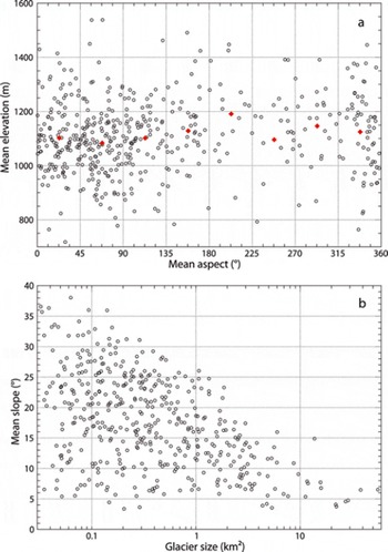
Fig. 8. (a) Variation of mean elevation with mean aspect of the glacier, both based on zonal calculations from the DEM. Red diamonds indicate mean values for each of the eight cardinal sectors. (b) Variation of mean slope (as derived on a pixel basis from the DEM) with glacier size in 1999.
Furthermore, a positive correlation, r = 0.81 (power law fit), between elevation range and glacier size is found (not shown) and a dependence of mean slope on glacier size is observed as depicted in Figure 8b. The upper boundary suggests the generalization ‘the larger the glacier the smaller the mean slope’, whereas the increasing variability towards smaller glaciers indicates that glaciers of the same size can have substantially different mean thickness values and thus glacier volumes (Paul and Svoboda, 2009).
Glacier-size changes
The analysis of the glacier size development from 1968 (N50) to 1999 (ETM+) reveals interesting details (Table 1; Figs 9 and 10). In total, for the sample of 300 glaciers there is a small decrease in glacier area (1.1%). Whereas the size class <1 km2 (mostly ice aprons) exhibits a small increase in overall size, the size class 1–5 km2 (mountain and small valley glaciers; Fig. 4b) exhibits a small area loss (2.4%). There is virtually no change in the 5–10 km2 class (mostly outlet glaciers), and glaciers larger than 10 km2 have slightly decreased, mostly due to three large glaciers calving in lakes. However, the scatter of individual changes is high, strongly increasing towards smaller glaciers (Fig. 9). Many glaciers <1 km2 have area gains in excess of 20% and some even increased their size by more than 60%.
Table 1. Glacier count, area covered, absolute and relative area changes, mean size and per cent of coverage per size class for the sample of 300 selected glaciers.


Fig. 9. Scatter plot of relative area change vs glacier size for the sample of 300 selected glaciers (eight glaciers smaller than 0.05 km2 are not shown). The red line segments give mean values per size class (Table 1).
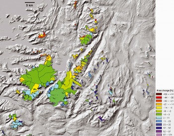
Fig. 10. Colour-coded illustration of the spatial variability of relative area changes from 1968 to 1999 for the southern part of the study region, depicting most of the 300 selected glaciers. The size of this region is 82 km × 72 km.
The geographic pattern of the area change is depicted in Figure 10 using a colour coding for the change value of each glacier (the intervals have been chosen to enhance the differences). The visual analysis reveals that the outlet glaciers of Vestisen and Østisen show (with a few exceptions) little area change. Some are smaller, others are larger than in 1968 and the total change is close to zero. Whereas most glaciers in the northwestern part (towards the coast) experienced a pronounced area decrease, many of the small glaciers in the eastern part of the scene exhibit increased sizes. As precipitation decreases further from the coast (Reference Østrem, Haakensen and MelanderØstrem and others, 1973), there must be a strong topographic control on the mass gain (e.g. snow accumulation by wind drift). However, no correlation of the changes with typical topographic parameters (e.g. slope, aspect) has been found. With regard to the three largest ice masses (Vestisen, Østisen and Blåmannsisen), their overall changes are less than 1% in each case and thus smaller than the mapping accuracy, which was assumed to be better than 5% for clean ice without interference from snow in previous studies (Reference Paul and KääbPaul and Kääb, 2005). However, in all three cases the small mean change is related to glaciers with a size increase that compensates the area loss of other glaciers.
Discussion
Methodological challenges
Whereas technical issues can be solved straightforwardly (e.g. manual correction of wrongly classified regions), the methodological issues (e.g. image selection, snow conditions and drainage divides) require some careful decisions. The most challenging tasks in this study were to separate seasonal snow from glaciers and distinguish seasonal from perennial snow. Whereas morphological considerations helped to separate the seasonal snow from the glaciers, the digitized glacier outlines from the N50 maps were used to identify possible perennial snowfields. By using different samples for the inventory and the change assessment, we were able to consider the different requirements for both datasets. However, we are aware that our glacier selection and ice-divide delineation is, to a certain extent, subjective and that it might have been treated differently by other analysts. Nevertheless, we are confident that our overall results will not change much due to different interpretations of individual glaciers.
The automated mapping from thresholded ratio images requires human inspection and subsequent correction of the generated glacier outlines in regions with debris cover, water and shadow. Only a few glaciers in this ice-cap-dominated region were corrected for debris cover or wrongly mapped outlines in shadow. Proglacial lakes occurred much more often and their correction was the most time-consuming facet of manual editing. Using identical drainage divides is mandatory when comparing the results with glacier extents reported in a former inventory. If the former inventory was compiled under adverse conditions (e.g. with seasonal snow outside glaciers) and digital glacier outlines are available (as in this study), it is advisable to digitize a separate glacier basin layer to calculate changes with respect to the same entities. When glacier outlines or printed maps are not available, a comparison is not recommended, as completely arbitrary changes might be calculated. For example, the different position of drainage divides as used for Atlas73 (Fig. 2) creates ‘virtual’ area changes of more than 50% for individual outlet glaciers of Blåmannsisen ice cap. It is thus mandatory to exactly refer to the same basins for any change assessment. Events like glacier split-up and disintegration might further complicate the change analysis (e.g. Reference CitterioCitterio and others, 2007; Reference DeBeer and SharpDeBeer and Sharp, 2007; Reference PaulPaul, 2007; Reference Andreassen, Paul, Kääb and HausbergAndreassen and others, 2008).
As reported in an earlier study (Reference Paul and KääbPaul and Kääb, 2005), the workload required for digitization of glacier basins is about the same as for correcting the glacier outlines themselves (lakes, debris, shadow). Both steps together account for more than 95% of the processing time, and only 5% or less is required for the effort related to the pre-processing of the satellite scene and selection of the correct thresholds for the classification. This implies that glacier outlines (corrected for lakes only) could be generated very quickly in regions with little debris cover on the glaciers.
Area changes
To be on the safe side, a large number of uncertain outlines (140 glaciers) were excluded from the area change analysis. The increasing scatter towards smaller glaciers (Fig. 9) might also reflect this uncertainty: the changes become more and more arbitrary. The three largest ice masses show very small relative area changes (<1%) compared with the extent from the N50 maps (for Blåmannsisen the N50 is from 1985). The analysis of the area changes thus reveals that the glaciers in this region are in a ‘healthy’ state and are still often close to their 1968 (or 1985) extent with an overall area change of −1%. In a comparable time period the area changes in the more continental Jotunheimen region, southern Norway, were −12% (164 glaciers) and have been increasingly negative towards smaller glaciers (Reference Andreassen, Paul, Kääb and HausbergAndreassen and others, 2008). Similar results have been obtained for many other regions around the world (Reference BarryBarry, 2006; Reference Granshaw and FountainGranshaw and Fountain, 2006; Reference DeBeer and SharpDeBeer and Sharp, 2007; Reference Racoviteanu, Arnaud, Williams and OrdoñezRacoviteanu and others, 2008a), indicating that the small changes of the Svartisen region are exceptional.
Also different from other regions of the world is the strong size increase of many small glaciers (<1 km2) causing a mean change close to zero for all small glaciers. Moreover, the general trend of increased size with larger distance from the coast is remarkable (Fig. 10). The reason for the strong area gains of individual small glaciers can only partly be explained by wrongly mapped snowfields in the N50 maps (see Fig. 4b). Overall, there is little doubt that many small glaciers were much larger in 1999 than in 1968. For example, nine glaciers are depicted as two entities on the N50 maps but have grown and merged to four units by 1999. Compared to an oblique aerial photography from 1985, we assume that a large part of the area gain must have occurred after 1985.
Some of the valley glaciers (either large or small) retreated considerably (300–500 m) during the 30 year period, although they are surrounded by smaller glaciers, which increased in size. However, some ice-cap outlet glaciers, such as the comparably large Engabreen, exhibited marked advance with a small relative area change, whereas other (smaller and steeper) outlet glaciers advanced less strongly but with a more pronounced size increase (see Fig. 10). The difference in the changes is also related to the width of the glacier front which is small for Engabreen but comparably wide for the small outlet glaciers. Hence, Engabreen is not necessarily representative of other glaciers in the region.
Interpretation
The abundant precipitation of the 1990s was closely correlated with positive mass balances at several Norwegian glaciers near the coast (e.g. Reference Nesje, Lie and DahlNesje and others, 2000). The mass gain resulted in advances for some of the large and steep outlet glaciers such as Engabreen, Nigardsbreen and Brikdalsbreen (Reference Andreassen, Elverøy, Kjøllmoen, Engeset and HaakensenAndreassen and others, 2005). Whereas for such glaciers the relation between climate forcing, mass-balance change and terminus response can be modelled and explained (e.g. Oerlemans, 2001), less is known about the reaction of smaller mountain or cirque-type glaciers to climatic change. The area gain observed in this study for numerous glaciers smaller than 1 km2 is thus difficult to explain. We speculate that local topographic characteristics might have helped to retain snow during the 1990s at the location of these small glaciers and finally resulted in the observed size increase. The highest relative area losses were found for glaciers in the wetter, northwestern part of the study site, whereas many of the glaciers that increased in size are located in the somewhat drier east. It seems that the behaviour of the glaciers in the Svartisen region is more controlled by local topographic factors (e.g. wind drift, radiation shielding) than by the large-scale variability in precipitation amounts.
Our results emphasize that glacier inventories should be repeated at intervals of a few decades to assess the overall changes, as the observed high variability and spatial pattern of the changes would not be revealed by a much sparser sample of field measurements. The analysis by Reference Andreassen, Kjøllmoen, Knudsen, Whalley and FjellangerAndreassen and others (2000) with a focus on length changes, mass balance and area changes of a few selected glaciers in this and other regions of northern Norway has already shown the strong regional variability.
Error assessment
The accuracy of the mapped glacier outlines is an important but difficult topic in glacier mapping from satellite imagery (e.g. Reference Hall, Bayr, Schöner, Bindschadler and ChienHall and others, 2003; Reference RaupRaup and others, 2007). Numerous error terms need to be considered for a sound assessment of the uncertainty in the derived area changes. Most of these errors have two parts: one that is comparably small and can be calculated by statistical means (technical error), and one that is large and difficult to assess (methodological or interpretation error). The former includes the orthorectification error of the satellite image and the digitizing error of the glacier outlines from a map. The latter includes the correct interpretation of debris-covered regions, seasonal/perennial snowfields (possibly attached to a glacier), and the position of ice divides in the accumulation area. Another type of error is related to the applied glacier-mapping algorithm, which is very small for clean to slightly dirty ice, but at the same time difficult to assess in absolute terms for at least two reasons:
-
1. A rigorous error calculation is only possible when adequate ground-truth data are available for comparison. Such data have to be acquired at the same point in time (due to highly variable snow conditions), with a similar sensor (including a shortwave, infrared band) and a better spatial resolution. These constraints are difficult to fulfil and previous estimates of mapping accuracy (e.g. better than 3% for clean ice) are based on a comparison of different datasets (e.g. SPOT pan with Landsat TM).
-
2. Generally, the automatically derived outline will be superior to manual delineation (for clean ice), because the applied spectral threshold value is consistent for the entire scene and the vector outlines are not generalized, i.e. they are reproducible and pixel sharp. This implies that they could not be validated against a ‘better’ ground truth.
Glaciers are fuzzy objects rather than sharp units and a certain amount of (optically thick) debris cover might be present on most (larger) glaciers. For this reason the automatically generated outlines are always compared and corrected against a ground truth (the original but contrast-enhanced satellite image) by visual interpretation. Consequently, the final outlines are not independent of the ground truth and classical accuracy measures do not apply. By using higher-spatial-resolution (but possibly panchromatic) data from the same point in time for comparison (Reference Paul, Huggel, Kääb, Kellenberger and MaischPaul and others, 2003), the critical decisions on the perimeter of each glacier are transferred to a higher number of pixels without necessarily generating more accurate outlines. Hence, quantifying the mapping accuracy is desirable but a statistically sound assessment is difficult to achieve and the methodological or interpretation error could be an order of magnitude larger.
In the Svartisen region, with mostly debris-free glaciers, the greatest error for the calculated size is introduced by the uncertainties in the separation from snowfields. Our best estimate is that this error can reach 25% for glaciers <1 km2 and may be 5–10% for glaciers >5 km2. For the transfer of the outlines to the GLIMS glacier database, we suggest adding an attribute that marks such highly uncertain (or only the relevant) glaciers. Considering rough figures from earlier studies of an overall mapping accuracy of 3–5% for ETM+ type sensors and clean ice (e.g. Reference Paul, Kääb, Maisch, Kellenberger and HaeberliPaul and others, 2002, Reference Paul, Huggel, Kääb, Kellenberger and Maisch2003; Reference Paul and KääbPaul and Kääb, 2005), the observed mean area changes in this study (in each size class and in total) are not significant. However, the area changes from a large number of individual glaciers are much larger than this uncertainty and should thus be realistic.
Conclusions
We have presented results from the new glacier inventory of the Svartisen region, including the methodological challenges, a statistical analysis of the inventory data and a calculation of area changes since 1968 for a selection of 300 glaciers. The major results from this analysis are:
Methodological issues are much more challenging and time-consuming than the glacier mapping itself, in particular the correct treatment of attached snowfields and assignment of drainage divides. Our conclusion is that considerable time should be spent selecting a satellite scene with the best snow conditions, and regions that suffer from too much seasonal snow should be excluded from statistical analysis. We recommend that appropriate pictures that illustrate the snow conditions in the analysed scenes be a part of all publications.
Human intervention is a most critical stage in the course of the glacier mapping: at first in the pre-processing (scene selection and threshold for classification) but mainly in the post-processing (manual editing and selection of samples for statistical analysis).
For clean glacier ice it is nearly impossible to find an adequate dataset that could be used for a sound error calculation. Moreover, the automatically derived glacier outlines will be in general (clean ice) superior to manual delineation as they are consistent throughout the entire scene and not generalized.
The previous glacier inventory in this region (Atlas73) was compiled from aerial photographs acquired under adverse snow conditions, and the delineation of glacier basins (ice divides) was sometimes very different. This makes a direct comparison of the changes complicated, as the ice divides could not be placed at the same location. Our recommendation is to digitize the glacier outlines from the former inventory and apply identical drainage divides to both datasets for the change assessment.
Drainage divides derived from bedrock topography could differ from those of the surface. For practical reasons (e.g. global availability), the latter should be used in separating individual glacier units. A flow-direction grid (or subsequent watershed analysis) derived from a DEM is very helpful for delineating the divides.
The overall area change since 1968 for a sample of 300 glaciers is close to zero in this region, and the size increase of ice aprons and small mountain glaciers (<1 km2) has compensated for the area loss of valley glaciers. The assumed influence of local topography on area changes implies that the small glaciers in this region are less sensitive to climatic changes than in other regions.
The size changes calculated in this study are difficult to compare with other regions as both the size class distribution (number and area covered) and the hypsography (ice caps) are different.
Future studies of glacier change in other parts of Norway may reveal whether the changes observed here are exceptional or not.
Acknowledgements
The work was supported by the Norwegian Space Centre as part of the Cryorisk project, by NVE and by the Norwegian Research Council as part of the Glaciodyn project. F. Paul was also partly supported by a grant from the European Space Agency project GlobGlacier (21088/07/ I-EC). J.E. Hausberg performed the quality check of the Landsat image orthorectification. We also thank H. Elvehøy for useful comments on the paper. Constructive reviews by an anonymous reviewer and T. Bolch improved the paper considerably.


