


Introduction
Bahía de Banderas on the Pacific coast of Mexico is known to be visited by the protected humpback whale (Megaptera novaeangliae) at various stages of its life cycle (Medrano-González et al., Reference Medrano-González, Peters, Vázquez, Álvarez, Ramírez and Nanduca2007). However, there has been an increase in vessel activity for various human uses in the bay (Noriega et al., Reference Noriega, Lecours and Medrano-González2023). The harmful effects of an increased number of vessels on areas used by marine mammal populations include, but are not limited to, vertical avoidance (increasing diving times), horizontal evasion (changing directions and/or speed), behavioural changes, and direct boat collisions (Au and Green, Reference Au and Green2000; Scheidat et al., Reference Scheidat, Castro, Gonzalez and Williams2004; Schaffar et al., Reference Schaffar, Madon and Garrigue2009; Rosenbaum et al., Reference Rosenbaum, Maxwell, Kershaw and Mate2014; Cunha et al., Reference Cunha, Freitas, Alves, Dinis, Ribeiro, Nicolau, Ferreira, Gonçalves and Formigo2017). Therefore, mapping whale distributions in space and time is essential to conservation in the face of increasing anthropogenic threats (Avila-Foucat et al., Reference Avila-Foucat, Sánchez Vargas, Frisch Jordan and Ramírez Flores2013).
Understanding the relationships between cetaceans and their environment can provide fundamental knowledge for the development of conservation strategies (Corkeron et al., Reference Corkeron, Minton, Collins, Findlay, Willson and Baldwin2011). Species distribution models (SDMs) are an important tool in the identification of critical habitats (Rasmussen et al., Reference Rasmussen, Palacios, Calambokidis, Saborío, Dalla Rosa, Secchi, Steiger, Allen and Stone2007; Corkeron et al., Reference Corkeron, Minton, Collins, Findlay, Willson and Baldwin2011; Marshall et al., Reference Marshall, Glegg and Howell2014). Critical habitats are defined as areas that provide a key value for the sustainability of a healthy population, including those used for raising calves (Hoyt, Reference Hoyt2005). SDMs have become a common approach to aid in the management of marine environments and decision-making processes (Smith et al., Reference Smith, Kelly and Renner2021). The widespread use of SDMs relies on the fact that they efficiently relate field observations of a species of interest to environmental predictor variables, or surrogates, using statistical probability (Guisan and Thuiller, Reference Guisan and Thuiller2005). Additionally, SDMs model presence-only data, which is particularly helpful when modelling highly mobile, rare, cryptic, or underwater species in environments where it may be more difficult (logistically and economically) to conduct systematic surveys and confirm true absences (Franklin, Reference Franklin2010; Smith et al., Reference Smith, Grantham, Gales, Double, Noad and Paton2012).
Humpback whales (Megaptera novaeangliae), a protected cetacean species under Mexican law (NOM-059-SEMARNAT-2010 and NOM-131-SEMARNAT-2010), are known for undertaking some of the longest migrations among mammals (Ransome et al., Reference Ransome, Frisch-Jordán, Titova, Filatova, Hill, Cheeseman, Bradford, Urbán, Martínez-Loustalot, Calambokidis, Medrano-González, Burdin, Fedutin, Loneragan and Smith2023). They spend the summer months (May–October) at high latitude feeding grounds and the winter (November–April) at low latitude breeding grounds (i.e. shallow tropical areas; Clapham and Mead, Reference Clapham and Mead1999). Typically breeding grounds are located in latitudes near 20°, in shallow areas with warm waters (Witteveen et al., Reference Witteveen, Worthy and Roth2009). In the North Pacific Ocean, the coast of Mexico has been recognized as the second most important breeding area for the Eastern North Pacific humpback whale subpopulation, harbouring approximately 40% of wintering individuals (Calambokidis et al., Reference Calambokidis, EA, TJ, AM, PJ, JK, CM, LeDuc, Mattila, Rojas-Bracho and JM2008).
The region of Bahía de Banderas, Mexico (Figure 1), constitutes a known breeding area for mating and calving activities (Medrano-Gonzalez et al., Reference Medrano-González, Peters, Vázquez, Álvarez, Ramírez and Nanduca2007). During the winter season, humpback whales are found primarily in the northern half of the bay, associated with the lee of the shore and the extended continental shelf (Medrano-González, Reference Medrano-González2009). It is widely known that humpback whale social organization and reproductive status determine habitat use in breeding areas (Craig and Herman, Reference Craig and Herman2000; Ersts and Rosenbaum, Reference Ersts and Rosenbaum2003; Smith et al., Reference Smith, Grantham, Gales, Double, Noad and Paton2012), and that the most vulnerable social groups to anthropic impacts are mother–calf pairs (MCP) (Oviedo and Solís, Reference Oviedo and Solís2008). The vulnerability of such social groups is explained by the fact that females with calves have shown a strong preference for shallow and sheltered waters close to the coastline (Ersts and Rosenbaum, Reference Ersts and Rosenbaum2003; Félix and Botero-Acosta, Reference Félix and Botero-Acosta2011). While habitat preference and use at a local scale may also be directly linked with the availability of suitable reproductive habitats (Rasmussen et al., Reference Rasmussen, Palacios, Calambokidis, Saborío, Dalla Rosa, Secchi, Steiger, Allen and Stone2007), there has been scarce research to identify, characterize, and map the critical habitat used by different humpback whale groups at this particular field site. Currently, the available information is based on individual sighting frequency (Arroyo-Sánchez, Reference Arroyo-Sánchez2017) and not on environmental preferences. Calving activities are mostly observed in the northern half of Bahía de Banderas, but these observations are anecdotal and no research has been done to explicitly link these observations with physical parameters of the environment to confirm this assumption beyond the initial analysis by Medrano-González et al. (Reference Medrano-González, Vázquez-Cuevas, Aguayo-Lobo, Salinas, Ladrón de Guevara-Porras and Peters-Recagno2010). It is essential to improve scientific understanding of the habitat requirements and specific features that breeding humpback whales are dependent upon within their breeding grounds (Smith et al., Reference Smith, Grantham, Gales, Double, Noad and Paton2012). Furthermore, increased coastal development and port infrastructure on the north end of the Bahia de Banderas has been shown to overlap with areas of high ecological importance for calving females (Pompa-Mansilla and Garcia, Reference Pompa-Mansilla and Garcia2017). In this context, the objective of this study was to identify and better understand the spatial distribution of critical calving habitat for humpback whales in Bahia de Banderas based on their spatial association with environmental characteristics.

Figure 1. Geographic location of all whale sightings recorded in the study area during the 2018–2023 breeding seasons. Dashed grey areas represent the seasonal marine protected area (MPA) designated for the protection of calving humpback whales. Red to blue lines represent the bathymetric contours starting at the 200 m isobath every 100 m depth interval. All whale sightings and data were projected into the World Geodetic System (WGS) 1984 Universal Transverse Mercator (UTM) Zone 13N.
Methods
Study site
Bahía de Banderas, in the states of Nayarit and Jalisco, is the third largest natural bay in Mexico, with a latitude (Figure 1) stretching from 20°15′ to 20°47′ N, and longitude from 105°15′ and 105°42′ W. The bay extends west of the Mexican Pacific coast and is divided in half by the mouth of the Ameca River. To the north it reaches to the headland of Punta Mita, Nayarit and in the south to Cabo Corrientes, Jalisco. Politically, the bay is shared by the municipalities of Bahía de Banderas in Nayarit and by Puerto Vallarta and Cabo Corrientes in Jalisco. Bahía de Banderas is divided by the 200 m isobath, demarcating the northern shallow half of the bay from the deep-water area to the south (also known as ‘The Banderas Canyon’). In the latter, the depth gradually increases towards the southwest until reaching >1400 m, just 0.25 nm (463 m) from the coast (Alvarez, Reference Alvarez2007). At the northern end of the bay, there is a seasonal marine protected area (MPA) – also known as the ‘Restricted Zone’ – where whale-watching activities are prohibited due to the concentration of whales with calves (Figure 1). This area is represented by a 2 km wide strip of coast extending from Punta Mita to the mouth of the Ameca River and around the Marietas Islands archipelago. The MPA is active throughout the duration of the whale-watching season, which is established and revised annually by Mexico's federal government (DOF, 2022), typically spanning from early December to late March. Additionally, the area has two natural protected areas (NPAs) inland, known as the Sierra Vallejo NPA to the north and the Mismaloya-Los Arcos NPA to the southeast, with a small portion encroaching into the eastern part of the bay's waters. Lastly, the seasonal MPA around the Marietas Islands is partially overlapped by a national park NPA known as the Parque Nacional Islas Marietas, encompassed by a rectangular polygon over and around the islands, but which does not explicitly relate to whales in its regulation.
Data
Whale sighting data were collected annually through non-systematic winter surveys conducted from small 24-foot vessels with outboard motors during the breeding seasons (November–April) from 2018 to 2023. The surveys were conducted in collaboration with the local non-governmental organization Ecología y Conservación de Ballenas A.C. (ECOBAC). The primary objective of these surveys was to collect photographs of humpback whale flukes for individual identification as part of an independent study. Location data were collected with a handheld global positioning system (GPS) receiver, and group composition was classified based on the number and size of the individuals and their behaviour classified based on previous research on humpback whale distribution in other breeding areas (Oviedo and Solís, Reference Oviedo and Solís2008; Félix and Botero-Acosta, Reference Félix and Botero-Acosta2011). Only the initial geographic position for each sighting was used for the analysis. The position was recorded when the vessel was located at a maximum distance of 30 m from the nearest whale, at the beginning of each sighting.
Following previous research on humpback whale characterization in other breeding areas (Oviedo and Solís, Reference Oviedo and Solís2008; Félix and Botero-Acosta, Reference Félix and Botero-Acosta2011), we classified groups into three social group categories based on observed behaviours. For example, instances where whales concurrently engage in competitive behaviour together in a coordinated fashion were considered a group, even if momentarily they were not physically close. The three defined groups were: MC groups (groups that included a calf and one or more adult whales), mating groups (MG; minimum group size of three whales, groups where at least two individuals engaged in physical competitive behaviours are following another whale), and other groups (OG); all whale sightings not included in the previous categories). We used the Kruskal–Wallis (Kruskal and Wallis, Reference Kruskal and Wallis1945) test and compared its results to a Wilcoxon–Mann–Whitney test (Mann and Whitney, Reference Mann and Whitney1952) to determine which groups were significantly different from each other based on different environmental variables.
Environmental variables at each sighting location were calculated using bathymetry from the GEBCO 2021 Grid. The GEBCO 2021 Grid provides global coverage of elevation data in metres on a 15 arc-second grid, which is equivalent to 430 × 430 m at the 20.8072° latitude. We retained this spatial resolution for all derived terrain variables and final model outputs. Twenty preliminary quantitative terrain variables were derived from the bathymetry dataset using the ArcGIS Pro 2.8.2 software and principles from geomorphometry (Lecours et al., Reference Lecours, Brown, Devillers, Lucieer and Edinger2016). Other than depth, the preliminary environmental variables related to the seafloor included: distance to coast, easterness and northerness, general curvature, local mean depth, mean curvature, local median depth, planar curvature, profile curvature, normal curvature, local range of depth, relative deviation from the mean depth, surface-to-planar area ratio, slope, statistical slope, local standard deviation of depth, surface area, tangential curvature, and a vector ruggedness measure (see Appendix, Table 2). These variables are frequently used in marine habitat mapping and species distribution modelling. They have been shown to directly or indirectly influence the distribution of numerous species, contingent on the species, environmental settings, and spatial resolution (McArthur et al., Reference McArthur, Brooke, Przeslawski, Ryan, Lucieer, Nichol, McCallum, Mellin, Cresswell and Radke2010; Harris and Baker, Reference Harris and Baker2020; Lecours et al., Reference Lecours, Brown, Devillers, Lucieer and Edinger2016; Misiuk et al., Reference Misiuk, Lecours and Bell2018; Lecours et al., Reference Lecours, Misiuk, Bucci, Prampolini and Araújo2024). Such resources have proven instrumental in informed decision-making pertaining to conservation and management efforts (Harris and Baker, Reference Harris and Baker2020). The correlation between the preliminary variables was evaluated using the Band Collection Statistics Tool available in ArcGIS Pro. The correlation matrix created enabled us to identify and filter out correlated variables (correlation coefficient greater than 0.7), keeping only uncorrelated variables and one variable of correlated pairs for analysis (no three variables or more were correlated together).
Complete spatial randomness
To evaluate clustering and estimate intensity of whale sightings, we performed two complete spatial randomness (CSR) tests. CSR is a type of statistical test determining whether events, in this case the location of whale sightings, are distributed independently and uniformly throughout a study area. Confirmation of CSR suggests that there are no specific regions where events are more or less likely to happen, and the presence of one event does not influence the likelihood of others nearby. Initially, we assessed CSR using a quadratic test, which measures the density of patterns across the study area. This test helps determine if the intensity of the pattern remains consistent throughout different locations within the study area. To conduct this evaluation, we utilized the ‘quadrat.test’ function from the ‘spatstats’ package (Baddeley et al., Reference Baddeley, Chang, Song and Turner2012) in R Statistical Software (version 4.2.1). This function divides the study area into grid quadrants and counts the number of points within each quadrant, comparing them to expected counts under the null hypothesis of CSR. The null hypothesis assumes that the probability of a point falling within each quadrant is proportional to the quadrant's area. The second test involved evaluating CSR by measuring distances from random events to their nearest-neighbouring events using Ripley's K test. This test assesses the conformity of the whale sightings point pattern to CSR by plotting the empirical function K(r) against the theoretical expectation and point-wise envelopes under CSR. These envelopes were generated by simulating a CSR point process in the study area (99 repetitions). Ripley's K function was calculated using the ‘kinhom’ function from the ‘spatstats’ package in R.
The first CSR test we performed was a quadratic test to assess if the local process intensity was constant across the study region independent of seafloor characteristics. This test measures the local density of a pattern in a study area, i.e., its density at different locations within the study area. To measure the local intensity of events, we employed the ‘quadrat.test’ function of the ‘spatstats’ package (Baddeley et al., Reference Baddeley, Chang, Song and Turner2012) in the R Statistical Software (v4.2.1). This function divides the study area into an irregular grid and counts the number of points that fall into each grid cell. These counts are then compared against the expected counts in a χ2 test under the null hypothesis of CSR, which states that the probability of a point falling into each quadrat is proportional to that quadrat's area. The second CSR test we performed was a Ripley's K test (Baddeley et al., Reference Baddeley, Møller and Waagepetersen2000). This test also measures the local density of a pattern, but it does so by measuring the distances from random events to their nearest-neighbouring event. Ripley's K test plots the empirical function K(r) against the theoretical expectation and point-wise envelopes under CSR by employing the statistical process developed by Baddeley et al. (Reference Baddeley, Møller and Waagepetersen2000). The point-wise envelopes were computed by repeatedly simulating a CSR point process with the same number of points as the pattern analysed in the study area performing 99 repetitions following the work of Leverett et al. (Reference Leverett, McLister, Desaivre, Conway and Boyd2022). The calculation of Ripley's K function was performed using the ‘kinhom’ function of the ‘spatstats’ package in R.
Seafloor influence on MC distribution
Depth, distance to coast, and slope have been widely identified as important factors to humpback whale MCP in other breeding areas (Ersts and Rosenbaum, Reference Ersts and Rosenbaum2003; Oviedo and Solís, Reference Oviedo and Solís2008; Félix and Botero-Acosta, Reference Félix and Botero-Acosta2011; Lindsay et al., Reference Lindsay, Constantine, Robbins, Mattila, Tagarino and Dennis2016). To assess the significance of the influence of these three variables on the spatial distribution of MC groups in the study area, we conducted a new series of quadrat tests. We reclassified the continuous data into five discrete classes for each proxy: five categories for depth, five categories of distance to the coastline, and slope, respectively. Categories were defined by distributing the observations equally across class intervals, giving the same frequency of observations per class. Subsequently, the resulting classes were incorporated into a dispersion test using the ‘quadrat.test’ function from the ‘spatstat’ package in R individually for each of the three seafloor proxies (see Appendix, Table A2).
To provide further insight into the relationships between these different proxies, we partitioned the MC sightings in the environmental space into clusters. These clusters represent the preference of the MC sightings in terms of the three proxies combined. This was done by conducting a K-means clustering analysis on all MC sightings. K-means clustering analysis uses an unsupervised machine learning algorithm to group data points into a number of user-specified clusters (K), such that the data points in each cluster are as similar as possible. We specified three clusters to group MC sightings to represent: the most common environmental preferences, a set of more extreme values at the edge of the niche, and outliers.
Calving habitat modelling
Among modelling approaches, the use of complex algorithms has been recognized as the most widespread (Radosavljevic and Anderson, Reference Radosavljevic and Anderson2014) and these have been successfully used to model cetacean habitats worldwide (Smith et al., Reference Smith, Grantham, Gales, Double, Noad and Paton2012; Lindsay et al., Reference Lindsay, Constantine, Robbins, Mattila, Tagarino and Dennis2016). As new modelling approaches are developed, there has been an ongoing debate on which is the best and how to choose one over another (Norberg et al., Reference Norberg, Abrego, Blanchet, Adler, Anderson, Anttila, Araújo, Dallas, Dunson, Elith, Foster, Fox, Franklin, Godsoe, Guisan, O'Hara, Hill, Holt, Hui, Husby, Kalas, Lehikoinen, Luoto, Mod, Newell, Renner, Roslin, Soininen, Thuiller, Vanhatalo, Warton, White, Zimmermann, Gravel and Ovaskainen2019). There remains no consensus, however, ensemble modelling may represent a potential solution (Zanardo et al., Reference Zanardo, Parra, Passadore and Möller2017; Claro et al., Reference Claro, Pérez-Jorge and Frey2020; Purdon et al., Reference Purdon, Shabangu, Yemane, Pienaar, Somers and Findlay2020). Ensemble modelling can be used to address some of the limitations of individual species distribution modelling approaches by combining the predictions of multiple models, which can reduce the overall bias and improve the accuracy of the predictions. Models can be combined by averaging the predictions of the individual models or by weighting the predictions according to their performance. A package in the software R, called ‘Stacked Species Distribution Model’ or ‘SSDM’, enables the implementation of ensemble modelling (Schmitt et al., Reference Schmitt, Pouteau, Justeau, de Boissieu and Birnbaum2017). The SSDM package allows the user to apply up to nine modelling algorithms over the same data to evaluate their performance and quantify their agreement. Using various algorithms over the same data provides a more robust approach to strengthening the outcome while not compromising the arbitrary exclusion of any individual algorithm. In the present study, we created two ensemble models. The first model included all whale groups recorded during the study period while the second model included only MC groups throughout the same time frame. We also created a monthly series to evaluate the temporal changes of this group during the entire winter season.
Humpback whale calving habitat was modelled using the SSDM package in R, testing the following algorithms: maximum entropy (MAXENT) (Hijmans et al., Reference Hijmans, Phillips, Leathwick and Elith2016), general additive model (GAM) (Wood, Reference Wood2006), generalized linear model (GLM) (R Core Team, Reference R2015), multivariate adaptive regression splines (MARS) (Milborrow, Reference Milborrow2016), classification tree analysis (CTA) (Therneau and Atkinson, Reference Therneau and Atkinson2015), generalized boosted model (GBM) (Ridgeway, Reference Ridgeway2015), artificial neural networks (ANN) (Venables and Ripley, Reference Venables and Ripley2002), random forests (RF) (Liaw and Wiener, Reference Liaw and Wiener2002), and support vector machines (SVM) (Meyer et al., Reference Meyer, Dimitriadou, Hornik, Weingessel and Leisch2015). Using this suite of algorithms, we associated the recorded whale occurrences to a set of environmental covariates derived from seafloor features. These included the variables explored in the dispersion tests (depth, distance to coast, and slope), as well as the uncorrelated selection from the 20 preliminary environmental variables described above. A total of 2000 pseudo-absence points were randomly generated in the SSDM package.
Despite the technique's widespread use, it is important when using presence-only data to acknowledge and address potential data limitations related to the non-systematic survey, which can be spatiotemporally heterogeneous and possibly biased towards easily accessible areas and times that present better navigation conditions (Corkeron et al., Reference Corkeron, Minton, Collins, Findlay, Willson and Baldwin2011) as well as the commercial basis of the navigation. The potential limitations of the data can be addressed by implementing spatial filtering and a good validation approach (Smith et al., Reference Smith, Kelly and Renner2021) such as the use of a geographic resampling parameter, which was used in the present study. A geographic resampling parameter can help reduce redundant or oversampled areas, and ensure a more balanced representation of different geographic regions or strata within the heterogeneous surveys.
The models for each algorithm were trained and validated using a holdout fraction of 0.7, with 0.7 of the occurrences used for model calibration and 0.3 for model validation (Huberty, Reference Huberty1994). Each individual model was selected to be included in the ensemble model if they had a Cohen's Kappa coefficient of at least 0.4 (i.e., at least moderate agreement; Landis and Koch, Reference Landis and Koch1977, Swets, Reference Swets1988), and an area under the receiver operating characteristic curve (Elith et al., Reference Elith, Graham, Anderson, Dudík, Ferrier, Guisan, Hijmans, Huettmann, Leathwick, Lehmann, Loiselle, Manion, Moritz, Nakamura, Nakazawa, Overton, Peterson, Phillips, Richardson, Scachetti-Pereira, Schapire, Soberon, Williams, Wisz and Zim2006) of at least 0.6. Variable importance was estimated based on Pearson's correlation coefficient between the model including all the provided variables and a series of models where each variable was omitted. The default parameters of the dependent R packages for each specific modelling algorithm were used. Ensemble model evaluation metrics (AUC, Cohen's Kappa coefficient, omission rate, sensitivity, and specificity) were all measured and based on a confusion matrix that summarizes the performance of the model's classification. We used the modelling process to create three distinct maps: one depicting the probabilities of occurrence per prediction grid cell, another illustrating inter-model agreement that serves as a map of uncertainty, and a binary map delineating suitable and non-suitable calving habitat pixels. The binarization was based on a probability threshold that maximized the true-skill statistics, as recommended by Liu et al. (Reference Liu, Berry, Dawson and Pearson2005) and Liu and Weng (Reference Liu and Weng2013) for presence-only data. The true-skills statistic (TSS) is a statistical measure of the accuracy of a species distribution model. It is a more robust measure than the AUC, as it takes into account the balance between sensitivity and specificity. We conducted two rounds of model runs: one preliminary and one final. The preliminary model was run with all kept variables and used to identify the variables with the greatest explanatory power. To simplify the models and improve interpretability, we removed variables that contributed minimally to the model variance. This step was necessary to reduce the risk of overfitting, which can occur when models include too many predictors (Townsend et al., Reference Townsend, Papeş and Eaton2007; Melo-Merino et al., Reference Melo-Merino, Reyes-Bonilla and Lira-Noriega2020) (see Appendix, Table A3). After the final model was run and the output was binarized into high-probability areas, we constructed a smoothed polygon using the Polynomial Approximation with Exponential Kernel (PAEK) interpolation method in the ‘smooth polygon’ tool in ArcGIS Pro 3.0.3 with a 700 m smoothing tolerance (corresponding to less than two pixels in the generated raster maps). Finally, to further understand the dynamic spatial distribution of calving groups over the breeding season within the study area, we classified the MC groups' sightings by month and repeated the process to produce a series of maps showing the probability of occurrence for each month. Additionally, we calculated the total area coverage identified as calving habitat by month and the number of MC sightings. To provide enhanced detail, each month's MC sightings were classified as MCP groups that included only a mother and calf, mother–calf–escort (MCE) groups that included a mother, calf accompanied by another large whale, and MCP defined as groups including a mother, calf, and two or more large whales (MCP + n).
Finally, we quantified the spatial overlap between the identified calving habitat and the seasonal MPA using ArcGIS Pro software. Initially, we created two polygons: one delineating the MPA area and the other mapping the identified calving habitat. Subsequently, we conducted a clipping procedure to retain only the overlapping areas, allowing us to quantify the total extent of calving habitat within the MPA. We then utilized this figure to calculate the proportion of the calving area covered by the MPA.
Results
A total of 1066 whale sightings were recorded across a total of 136 boat trips which collectively accounted for 836 survey hours during the study period (2018–2023). Efforts were made to ensure comprehensive coverage of the bay in a relatively uniform manner; 242 of these sightings were MC groups, 109 were classified as mating groups (MG), and the remaining 715 were classified as other groups (OG) which encompassed all other wintering activities (Figure 1). The results of the CSR test showed a significant deviation (P < 0.05) from the null hypotheses of CSR with a significant clustering at shorter distances and significant dispersion at larger distances from the coast (see Appendix, Figure A2).
The Kruskal–Wallis and Wilcoxon tests detected significant (P < 0.05) differences between the spatial distribution of MC groups and the other groups (Figure 2) based on the depth, distance to the coast, and slope. The mean depth over which MC groups were sighted was 56 m at a mean distance from the coast of 2.1 km and a mean slope of 1.6°. The mean depth and distance to the coast for MG were 126 m, 4.5 km respectively and 1.8° mean slope. Lastly, OG sightings were sighted at a mean depth of 146 m, 3.6 km from the coast and 2.3° of slope.
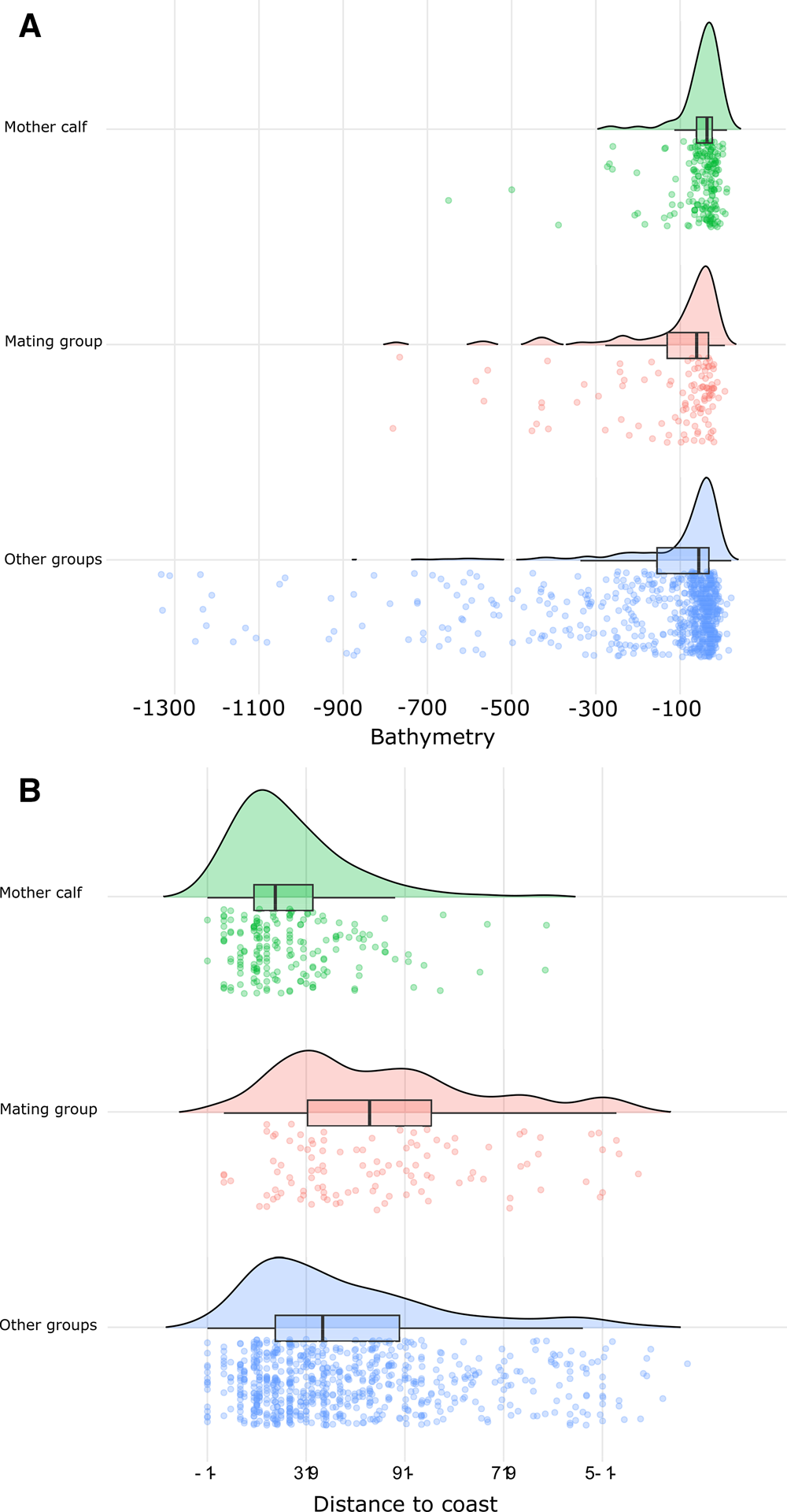
Figure 2. Humpback whale sighting density by social group relative to sea depth (bathymetry) measured in metres (A) and distance to coast measured in km (B). Curves and boxplot illustrate the distribution of sighting density by social group relative to the two seafloor proxies. Jittered data points represent individual sightings.
Seafloor influence on MC groups
A total of 242 MC groups were recorded during the study period, 156 of which were classified as MCP, 73 as MCE groups, and 13 as MCP + n (Figure 3). The dispersion test for each of the three seafloor proxies (depth, distance to coast and slope) detected a significant relationship (P < 0.01) between the number of MC groups and each of the covariates.
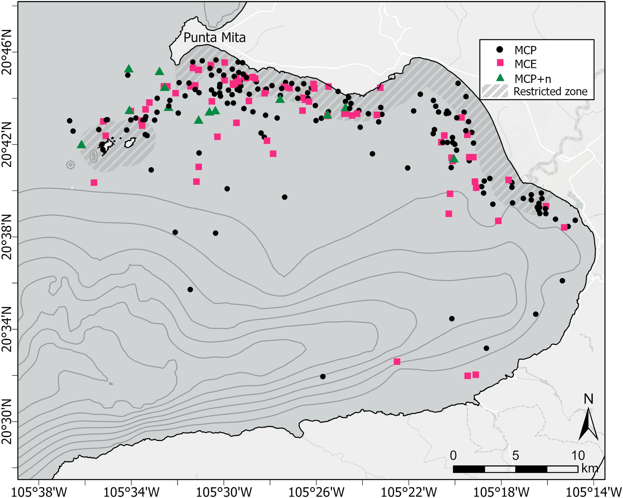
Figure 3. Distribution of humpback whale MC sightings in Bahia de Banderas, Mexico during the breeding seasons of 2018–2023. Black dots represent mother–calf pairs alone (MCP); squares represent mother–calf-escort groups (MCE) and triangles represent MCP with two or more other whales (MCP + n). Thin dark grey lines represent the bathymetric contours starting at the 200 m isobath every 100 m depth interval. Thick dashed grey areas represent the seasonal marine protected area (MPA) designated for the protection of calving humpback whales.
Results from the K-means clustering analysis suggested that the largest cluster encompassed 83.6% of the total MC points; its centroid calculated at a depth of 37 m, a distance of 1.9 km from the coast, and at a slope of 1.4°. The next largest cluster encompassed 14.8% of the total MC points; its centroid was calculated at a depth of 188 m, a distance of 3.4 km from the coast and a slope of 4.4°. Finally, the last cluster encompassed a mere 1.6% of the points; had its calculated centroid at a depth of 630 m, a distance of 5.4 km from the coast and a slope of 10.4°.
Modelling calving habitat
The correlation analysis of the preliminary variables identified nine uncorrelated variables (depth, distance to coast, easterness, northerness, profile curvature, relative deviation from the mean depth, slope, statistical slope, and tangential curvature) to be used in the preliminary model run (see Appendix, Table A3). We then evaluated variable contribution during the preliminary run to quantify and retain four variables that contributed at least 13% to the explanatory power of the preliminary model which appeared to be a natural threshold between those variables that contributed a lot and those that contributed little to the model (see Appendix, Table A4). The four retained variables and their respective percentages of explained variance in the final model run were distance to coast (46.0%), slope (23.6%), depth (17.0%), and profile curvature (13.4%).
Based on the evaluation metrics for the generated ensemble distribution model for humpback whale calving groups in the studied geographic space (Table 1), predictions showcased notable consistency with observed data, and its performance could be categorized as having a moderate agreement (Landis and Koch, Reference Landis and Koch1977, Swets, Reference Swets1988). The identified threshold set to be the probability that maximizes the true-skill statistics was determined at 0.36. The present study effectively identified three areas with high breeding habitat suitability values within the study area, based on physical characteristics of the seafloor (Figure 4). These calving areas can be conceptualized as: a large (261.8 km2) area on the north end of the bay, extending from the coastline out to approximately 4.5 km from Punta Mita to the Eastern edge of the bay, as well as two smaller (9.5 and 5.4 km2) areas on the southern coast of the bay that stretch approximately 2.5 km from the coastline (Figure 4).
Table 1. Ensemble model evaluation metrics

Area under the receiver operating curve (AUC), omission rate, sensitivity, specificity, proportion of correctly predicted presences, and Cohen's Kappa coefficient, based on a confusion matrix summarizing the performance of the model's classification.

Figure 4. Distribution of identified suitable breeding habitat. (A) Mapped breeding habitat suitability of humpback whale breeding behavior based on the ensemble SDM model. Darker blue shades represent higher breeding habitat suitability. Dashed grey areas represent the seasonal marine protected area (MPA) designated for the protection of calving humpback whales. (B) Binary map of humpback whale suitable calving habitat in dark blue based on a 0.36 binarization threshold. Non-suitable area is depicted as the remaining grey area of the bay's waters. Dark grey lines in the represent the bathymetric contours starting at the 200 m isobath every 200 m depth interval. Dashed grey areas represent the seasonal marine protected area designated to protect calving humpback whales. *According to the Mexican Ministry of the Environment and Natural Resources (Secretaría de Medio Ambiente y Recursos Naturales).
Seasonal changes over critical habitat use
The spatial distribution of MC groups was evaluated by each month of the breeding season when the groups were sighted. The number of MC group sightings had its peak during the month of March, with a total of 108 MC groups, represented by 74 MCP, 28 MCE and 6 MCP + n (Figure 5). The lowest number of calving-group sightings was recorded during the month of November with only three sightings in total represented by 1 sighting of MCP, 1 of MCE, and 1 MCP + n. The total area classified as high probability of occurrence within the study area decreased as the number of MC groups increased (Figure 6). Due to the low number of sightings during the month of November, it was not possible to model the probability of occurrence for this month accurately.
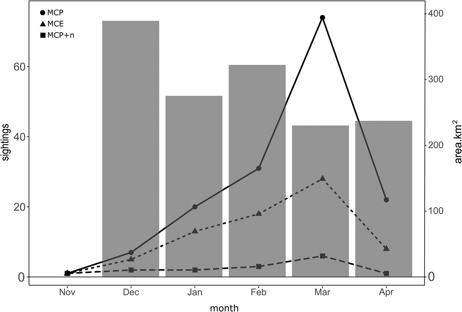
Figure 5. Seasonal occurrence of humpback whale groups containing a MCP during the breeding seasons from 2018 to 2023 in Bahía de Banderas, Mexico. The total number of sightings by group (left y-axis). Black dots represent mother–calf pairs alone (MCP); triangles represent mother–calf pairs escorted (MCE), and squares represent MCPs with two or more other whales (MCP + n). Grey bars represent the total area of high probability of occurrence based on a 0.36 binarization threshold by month (right y-axis).

Figure 6. Mapped breeding habitat suitability of humpback whale breeding behaviour based on the ensemble SDM model by month of the breeding season in Bahía de Banderas, Mexico. (A) Represents the estimated probability of occurrence during the month of December, (B) January, (C) February, (D) March, (E) April. Darker blue shades represent higher breeding habitat suitability. The month of November is excluded since the low number of calves sighted did not permit suitable habitat to be modelled. (F) Cumulative high suitability value areas across all months of the breeding season, i.e., how many months each pixel is suitable breeding habitat (pink areas represent those with the highest cumulative suitability across all months). Dark grey lines represent the bathymetric contours starting at the 200 m isobath every 100 m depth interval. Dashed grey areas represent the seasonal marine protected area designated for the protection of calving humpback whales.
The effect of the changes in the inter-seasonal distribution of MC groups was noticeable in the monthly SDMs performance, where the models increased their performance in all measured metrics (Table 2) during the last two months of the winter season.
Table 2. Model evaluation metrics by month

Area under the receiver operating curve (AUC), omission rate, sensitivity, specificity, proportion of correctly predicted presences, and Cohen's Kappa coefficient, based on a confusion matrix summarizing the performance of the model's classification.
We identified a visible spatio-temporal distribution pattern where calving mothers tend to restrict their occurrence to the calving area on the northern end of the bay as the breeding season progresses (Figure 6). Finally, we identified areas of cumulative high suitability values throughout the breeding season (panel F in Figure 6). Our findings underscore the significance of the northern portion of the bay across all months examined, contrasting with the variable suitability values observed in southern areas, which exhibit high suitability, but only during certain months of the breeding season.
Discussion
Humpback whale distribution
Humpback whale habitat use in the breeding grounds is dependent on the social organization and reproductive status of individuals (Craig and Herman, Reference Craig and Herman2000; Ersts and Rosenbaum, Reference Ersts and Rosenbaum2003; Oviedo and Solís, Reference Oviedo and Solís2008; Smith et al., Reference Smith, Grantham, Gales, Double, Noad and Paton2012). Our results describe a distinct spatial distribution pattern for the three social groups, characteristic of humpback whales, where calving mothers are present in the shallower waters and exhibit more restricted spatial preferences relative to other social groups in other wintering areas around the world (Smultea, Reference Smultea1994; Guidino et al., Reference Guidino, Llapapasca, Silva, Alcorta and Pacheco2014) as well as previous findings in Bahia de Banderas (Medrano-González et al., Reference Medrano-González, Vázquez-Cuevas, Aguayo-Lobo, Salinas, Ladrón de Guevara-Porras and Peters-Recagno2010).
Most humpback whales are found within the 200 m isobath regardless of their social organization or reproductive status (Smith et al., Reference Smith, Grantham, Gales, Double, Noad and Paton2012; Guidino et al., Reference Guidino, Llapapasca, Silva, Alcorta and Pacheco2014), with calving mothers documented to inhabit areas closer to the coastline with shallower waters relative to other social groups (Craig and Herman, Reference Craig and Herman2000; Félix and Botero-Acosta, Reference Félix and Botero-Acosta2011; Smith et al., Reference Smith, Grantham, Gales, Double, Noad and Paton2012). Our study showed a general positive tendency towards increasing whale sightings at distances under 5 km from the coast and depths shallower than 200 m for all the social groups. The presence of a socially segregated distribution pattern is a characteristic feature of breeding and calving areas (Guidino et al., Reference Guidino, Llapapasca, Silva, Alcorta and Pacheco2014), and the fact that social groups relating to different wintering activities (not calving) could not be modelled with accuracy based on physical seafloor characteristics highlights the widespread distribution of these groups in the study area.
Distribution of MC groups
Our findings on calving habitat preferences add to the understanding of Bahía de Banderas as a crucial breeding site for the Eastern North Pacific subpopulation (Medrano-González et al., Reference Medrano-González, Peters, Vázquez, Álvarez, Ramírez and Nanduca2007), which has been described to hold substantial significance for the phylogeographic structure of the species because of its isolation from humpback whales of other North Pacific subpopulations (Medrano-González et al., Reference Medrano-González, Baker, Robles-Saavedra, Murrell, Vázquez-Cuevas, Congdon, Straley, Calambokidis, Urbán-Ramírez, Flórez-González, Olavarría-Barrera, Aguayo-Lobo, Nolasco-Soto, Juárez-Salas and Villavicencio-Llamosas2001).
Seafloor influence on MC distribution
The present study effectively detected influences of bathymetric features on the spatial distribution of calving groups. Calving groups in the area of study were sighted at a mean depth of 59 m, 2 km from the coastline and on a 2° slope. These are consistent with the documented preferences for the species in other breeding areas globally, such as eastern Australia (Smith et al., Reference Smith, Grantham, Gales, Double, Noad and Paton2012), Costa Rica (Oviedo and Solís, Reference Oviedo and Solís2008), and Ecuador (Félix and Botero-Acosta, Reference Félix and Botero-Acosta2011). The preference of shallow coastal waters likely represents a behavioural response aimed at decreasing the risk of predation and reducing harassment by sexually active males (Craig and Herman, Reference Craig and Herman2000).
It is worth noting that, during the present study's fieldwork, we documented a distinctive calving sighting during the 2021 winter season. This sighting, which occurred at the unusual depth of 388 m and far from the coast (6.9 km), involved a pod of orca whales (Orcinus orca) actively trying to separate a humpback whale calf from its mother and drown it. Incidents of predatory attacks by orcas on humpback whales in this region have been documented for the past decade. While the exact frequency of these attacks is unclear, anecdotal accounts from vessel captains suggest a possible increase in recent years. We suggest that calving mothers have been affected by the rapid coastal development occurring in the coastal areas to the north and northeastern extremes of the bay, adjacent to the identified critical habitat area for calving whales (Medrano-González et al., Reference Medrano-González, Peters, Vázquez, Álvarez, Ramírez and Nanduca2007). This might have triggered a reported movement to areas outside of the bay that may be less suitable for calving where calving whales are more vulnerable to predation and other risk factors such as entanglement and vessel collisions (Medrano-González et al., Reference Medrano-González, Peters, Vázquez, Álvarez, Ramírez and Nanduca2007).
Studies on other North Pacific breeding grounds have found that the occurrence of MC groups can be influenced beyond the direct effects of depth and distance to the coast (Craig and Herman, Reference Craig and Herman2000). The combined effect of these two variables can be depicted by the seafloor slope which plays an important role in calving mothers' habitat preferences. Our study showed a marked preference for shallow slopes (around 2°) across all social groups. Similar environmental preferences were reported in Hawaii, where humpback whales favoured areas within the 200 m isobath and less steep slopes (Craig and Herman, Reference Craig and Herman2000); humpback whales seem to prefer calving grounds with gentler slopes. This might explain the higher calving frequency in the northern end of Bahía de Banderas. The southern end of the bay has a much smaller area with water depths below 200 m deep, where, unlike the northern end, the water depth increases rapidly as a function of distance from the coast offering fewer suitable calving sites with gentle slopes. Contrastingly, a study conducted in the South Pacific did not find a clear preference relating to slope, which could be explained by the fact that the authors report a ‘relatively homogeneous’ seafloor slope in their study area (Smith et al., Reference Smith, Grantham, Gales, Double, Noad and Paton2012). Bahía de Banderas, on the other hand, has a stark contrast in bathymetry between the north and south ends of the bay; with the north end of the bay resembling an extended continental platform with a gentle slope and the south increasing in depth at shorter distances from the coast (Figure 1). At a breeding ground with similar contrasting bathymetric characteristics, off the west coast of Africa, research reported a preference for shallow waters with the exact same slope preference of 2° (Chou et al., Reference Chou, Kershaw, Maxwell, Collins, Strindberg and Rosenbaum2020). These similar results could indicate that the relevance of slope in the distribution of calving humpback whales is dependent on the presence of contrasting bathymetric features within the breeding ground. This preference for gentle seafloor slopes might be associated with a more suitable environment for calves, offering protection and potentially making navigation easier for the young whales. However, this hypothesis is as yet untested by means of behavioural observations, so it is possible that slope may also be a surrogate for resource gradients that drive more directly whale distributions.
Furthermore, factors beyond the scope of this study, such as wind and waves, which directly influence sea state, could further explain the whales' preference for the northern part of the bay. The north offers shelter from these factors, while the southern end of Bahía de Banderas remains more exposed. Water temperature has also been a variable reported to influence the distribution of calving humpback whales, however, it has been suggested that its influence is outweighed by the topographic features that offer suitable shallow, protected conditions that can be used even with suboptimal temperatures (Smith et al., Reference Smith, Grantham, Gales, Double, Noad and Paton2012). Nevertheless, it is important to mention that while our modelling would undoubtedly benefit from the inclusion of temperature data, such data were not available for this area at a resolution suitable for inclusion in the models.
Modelling calving habitat
Species distribution models are computational tools used to predict the potential geographic distribution of a species based on environmental variables (Cañadas et al., Reference Cañadas, Sagarminaga, De Stephanis, Urquiola and Hammond2005). These models aim to understand and predict where a species is likely to occur based on its observed presence or absence in relation to environmental conditions (Austin, Reference Austin2007). The distribution model presented here identified a high probability of occurrence in shallow coastal areas represented by three identified zones: the first, a large (261 km2) area that spans from the northern end of the area of study, Punta Mita, running along the lee shoreline until reaching the easternmost part of the bay in an area adjacent to the large urban centres. Additionally, two identified areas of 9.5 and 5.4 km2 located nearly parallel to the southern coast and separated from the shoreline by 50–1000 m. It is worth mentioning that these last two areas were significant only for some months of the breeding season, as opposed to the larger northern area which remained important throughout the winter. All three identified areas are consistent with previously reported high-density calving whale sighting areas in the bay, based on long-term sampling efforts conducted by the National Autonomous University of Mexico since the early 1980s (Arroyo-Sánchez, Reference Arroyo-Sánchez2017).
The more protected shallow waters in the identified areas provide calving mothers with sea conditions that presumably allow for less energy expenditure for both the newly born calves (Oviedo and Solís, Reference Oviedo and Solís2008) and the lactating females. This protected environment likely serves as a critical resting habitat before migration. Lactation and pregnancy can exhaust up to 19% of total energy stores in mature whales (Lockyer, Reference Lockyer2020). Therefore, the duration of stays within the breeding grounds before migrating is critically important for energy expenditure, particularly, in a high proportion of females that are simultaneously lactating and pregnant (Pallin et al., Reference Pallin, Baker, Steel, Kellar, Robbins, Johnston, Nowacek, Read and Friedlaender2018). Improved understanding of the seasonal usage patterns in this breeding ground will help improve management strategies focused on this vulnerable social group enabling the maintenance of optimal environmental conditions needed by calving whales. Additionally, the fact that non-calving groups were unable to be modelled with environmental conditions in the area of study is an important fact to consider when designing management strategies that aim to include such groups. The widespread distribution of non-calving humpback whales across the bay highlights the need for the development of alternative management strategies beyond the designation of a localized partial area.
Calving whales and management implications
Calving mothers represent the most vulnerable group to anthropic impacts (Félix and Botero-Acosta, Reference Félix and Botero-Acosta2011) and are therefore a management priority. The knowledge generated here has the potential to aid management strategies, such as local MPA designations based on the determination of critical habitat (Oviedo and Solís, Reference Oviedo and Solís2008). Critical habitats are defined as areas that have a key value for the sustainment of a healthy population, including those used for raising calves (Hoyt, Reference Hoyt2005), such as the ones identified here. Currently, local protection is represented by a seasonal MPA designated by the Mexican Official Normativity NOM-131-SEMARNAT-2010 to protect calving mothers. This MPA overlaps 34.4% of the critical habitat identified in the northern end of the bay. The MPA is defined as a 2 km swath from shore and a 1.5 km band around the two Marieta Islands at the northern extreme of the bay without considering the remaining calving area along either the northern or the southern critical habitat detected in the present study and by Arroyo-Sánchez (Reference Arroyo-Sánchez2017). Similar spatial discrepancies between areas designated under some kind of protection and those highly used by calving humpback whales have been reported in other breeding sites where the limited levels of protection by regulation of human activities like marine traffic and tourism render calving whales more susceptible to potential disturbances and collisions (Devillers et al., Reference Devillers, Pressey, Ward, Grech, Kittinger, Edgar and Watson2020). In the past, it has been recognized that one of the most important threats to breeding whales in Bahía de Banderas is represented by collision with vessels (Medrano-González et al., Reference Medrano-González, Peters, Vázquez, Álvarez, Ramírez and Nanduca2007). While there is currently limited explicit information on the probability of collision at the local level, it is known that a heavily used area for navigation is represented by a southern marine corridor that connects the communities at the southern extreme of the bay (Noriega et al., Reference Noriega, Lecours and Medrano-González2023). An overlapping analysis with the data presented here is a logical next step that could lead to the estimation of high probability of humpback whale and vessel co-occurrence. A previous study by Smith et al. (Reference Smith, Grantham, Gales, Double, Noad and Paton2012) used a similar modelling approach to identify suitable breeding habitat for humpback whales in the Great Barrier Reef. They found ‘potentially important’ wintering areas for humpback whales located near major designated shipping routes. The present study shows a similar pattern in our study area – where suitable breeding habitats for whales seem to be located near areas with high vessel traffic (as also suggested by Noriega et al., Reference Noriega, Lecours and Medrano-González2023). Management efforts should take this knowledge as an opportunity to enhance conservation strategies by including all identified calving habitats. The use of species distribution models as a tool to aid in the identification of potential MPAs for marine mammals has been proven as feasible and effective, providing improved knowledge over distribution maps based on individual occurrences or encounter rates (Cañadas et al., Reference Cañadas, Sagarminaga, De Stephanis, Urquiola and Hammond2005).
Limitations and considerations
While trained biologists performed observations for this study, and the results are reported based on the predicted habitat suitability and not on the sighting points directly, it is important to caution about the potential bias introduced in our study. Because we used data obtained from whale-watching boats where searching effort is biased towards groups with coastal distributions or higher surface activity the study area was not surveyed homogeneously. SDMs trained on presence-only data exhibit a higher propensity for false-positive predictions compared to those trained on true presence–absence data. This increased susceptibility stems from the inherent inability of presence-only SDMs to distinguish between true absences and areas where the species has not been observed, a characteristic particularly prevalent in marine mammal sampling. Careful consideration is advised because false positives can pose significant challenges in conservation planning, potentially leading to the misallocation of resources and the protection of areas that are not essential for the species' survival. This phenomenon is exemplified in the identification of southern areas characterized by physical conditions deemed highly suitable by the model. However, the exclusion of crucial factors, such as exposure to wind and wave action due to geographical orientation, might make southern areas seem ideal based on some factors, but they could be too exposed to harsh weather, making them less valuable than the northern areas.
By recognizing the biases present in species occurrence data, analytical methodologies can deliberately incorporate them, allowing for appropriate adjustments and discounting of excessive influence (Boakes et al., Reference Boakes, McGowan, Fuller, Chang-qing, Clark, O'Connor and Mace2010). Since our survey data was expected to oversample easily accessible coastal areas, we addressed these likely concerns by implementing a geographic resampling, which was designed to mitigate issues related to redundancy and oversampling within geographical regions, thereby fostering a more equitable representation of distinct geographic zones within the area of study. The performance of our model was poor when attempting to model other social groups. This is likely due to sampling bias, as our data set was not representative of these groups. Future work in this area would benefit from the inclusion of survey effort distribution data that could subsequently rectify the sighting intensity metric associated with the whale attribute of interest.
Conclusions
Despite the biases given by the heterogeneity of effort, predictive habitat modelling succeeded in showing the spatial distribution of humpback whale calving pods in Bahía de Banderas, Mexico. Our results agree with those from other studies, both within this region and other regions world-wide and add additional insights via new finding. Humpback whales in Bahía de Banderas exhibit a distinct spatial distribution pattern, with calving mothers preferring shallower waters closer to the coast than other social groups. This study identified three areas with a high probability of occurrence for calving whales in Bahía de Banderas: a large area at the northern end of the bay stretching east in a funnel-like shape until reaching the central bay, and two smaller areas mostly separated from the coast at the southern extreme. The delineation of these areas could be used to improve current management strategies based on calving habitat.
Calving habitat use in Bahía de Banderas exhibits a marked seasonal pattern, characterized by a dispersed distribution across the bay during the early months of the breeding season and a gradual concentration within designated calving areas towards the end.
The knowledge generated in this study confirms the area's importance as a breeding ground for the eastern North Pacific humpback whale subpopulation.
The results presented here represent new and valuable analytical approaches to explicitly characterize the spatial distribution and critical habitat of calving humpback whales based on physical characteristics within the Bahía de Banderas area (depth, slope, curvature, and distance to coast). However, it is important to consider these results carefully as habitat utilization is contingent upon quantitative assessments extending beyond mere presence data. Future research would benefit from considering factors such as the spatial dispersion of survey endeavours and temporal fluctuations. A logical next step to the research presented here would be to incorporate information regarding the distribution of human activities in the sea and its influences from land to conduct an overlapping analysis and identify potential areas of conflict where management strategies could be directed and focalized.
Supplementary Material
The supplementary material for this article can be found at https://doi.org/10.1017/S0025315424000821.
Data
Data will be made available by the corresponding author on request.
Acknowledgements
This work would not have been possible without the Mexican National Council of Science and Technology providing the scholarship to author Fernando Noriega-Betancourt to attend the Interdisciplinary Ecology PhD program at the University of Florida. We express our deepest gratitude to the unwavering commitment of the ECOBAC field research team, whose ongoing research and survey efforts have been instrumental to the success of this project. We also extend our sincere appreciation to all dedicated members of ECOBAC, whose steadfast support and tireless dedication have not only been integral to the project's success but have also played a pivotal role in the preservation of local whale conservation for over three decades, to Karel Beets and Ecotours de Mexico for their invaluable logistical assistance and support during the fieldwork phase. We extend our sincere appreciation to the thesis committee members Dr Bette Loiselle and Dr Jessica Kahler. Additionally, we express our gratitude to Dr Angélica Almeyda, for her counsel during the early stages of manuscript development. This research's fieldwork was conducted under research permits SEMARNAT: SGPA/DGVS/011589/17 to SPARN/DGVS/03807/23. Finally, we are grateful to Joshua Doby and Audrey Wilson for their invaluable assistance in revising the text for English language clarity.
Author Contributions
Fernando Noriega: Conceptualization, Data curation, Formal analysis, Investigation, Methodology, Visualization, Writing – original draft, Writing – review & editing. Vincent Lecours: Conceptualization, Investigation, Methodology, Resources, Supervision, Writing – review and editing. Astrid Frisch Jordán- fieldwork data collection and review, Luis Medrano-González: Writing – review and editing.
Financial Support
This research received no specific grant from any funding agency, commercial or not-for-profit sectors.
Competing interest
None.
Ethical Standards
Research Ethics comply with international standards and with laws and regulations of Mexico. This research's fieldwork was conducted under research permits SEMARNAT: SGPA/DGVS/011589/17 to SPARN/DGVS/03807/23.


 Open access