

1 Introduction
The data preprocessing always has an important effect on the generalization performance of a supervised machine learning (ML) algorithm. By taking into consideration that well-known and widely used methods of ML often involved in data mining (DM), the importance of the data preprocessing in DM can be easily recognized. In general, ML is concerned with predicting an outcome given some data (Witten et al., Reference Witten, Frank, Hall and Pal2016). Many ML methods can be formulated as formal probabilistic models. Thus, in this sense, ML is almost the same as statistics, but it differs in that it generally does not take care of parameter estimates (just for predictions) and it is focused on computational efficiency (Witten et al., Reference Witten, Frank, Hall and Pal2016). DM is a field that is based on various approaches of ML and statistics and it is accomplished by an expert on a specific dataset with a desired result in mind (Witten et al., Reference Witten, Frank, Hall and Pal2016). In many cases, the dataset is massive, complicated or it is possible to have particular problems, for example, when there are more features than instances. In general, typically, the aim is either to generate some preliminary insights related to an application field where there is little a priori knowledge, or to be able to predict accurately future observations.
In many problems, the dataset that it has to be managed contains noisy data which makes the elimination of noisy instances necessary and one of the hardest processes in ML (Zhu & Wu, Reference Zhu and Wu2004; van Hulse & Khoshgoftaar, Reference van Hulse and Khoshgoftaar2006; van Hulse et al., Reference van Hulse, Khoshgoftaar and Huang2007). Another difficult issue is the distinguish among inliers and true data values. These values (inliers) are error data values that can be found in the interior of a statistical distribution and their localization and correction constitutes a very difficult task. Thus, although the multivariate data cleaning constitutes a complicate procedure, it is necessary, efficient and effective process (Escalante, Reference Escalante2005).
A common problem that has to be tackled by utilizing data preparation is the handling of the missing data (Pearson, Reference Pearson2005; Farhangfar et al., Reference Farhangfar, Kurgan and Pedrycz2007). In many cases, various datasets that contain both numerical and categorical data have to be handled. On the other hand, it is well-known that many algorithms, such as the logic learning algorithms, can handle better or exhibit a better performance only with categorical instances. In the case that it occurs, the discretization of numerical data constitutes a very important issue (Elomaa & Rousu, Reference Elomaa and Rousu2004; Flores et al., Reference Flores, Gámez, Martnez and Puerta2011). A very useful approach for handling the above problem is the grouping of the categorical data. As a consequence, the original dataset is transformed from categorical to numerical. From another point of view, a dataset with many different types of data or many values is difficult to be handled. This raises questions such as, which set of data gives the most useful information and therefore which amount should be chosen for inducing decision trees or rule learners? As a natural consequence, there may be a serious risk of overestimating much of the data, which makes the selection process of the most informative features a very difficult task. A well-known and widely used technique through which this normal learning difficulty is covered from very large datasets is the selection of a sample data from the initially large dataset (Wilson & Martinez, Reference Wilson and Martinez2000). On the other hand, the question remains and is pertinent, which sample is appropriate to choose or how large does this subset of data need to be? Various techniques have been proposed to solve the issue of imbalanced data-classes (Batista et al., Reference Batista, Prati and Monard2004; Estabrooks et al., Reference Estabrooks, Jo and Japkowicz2004), but it still remains a problem that requires further study.
The data preprocessing steps with which we will deal in the paper at hand is exhibited in Figure 1. In particular, the flow that is followed before applying the learning algorithms to a particular DM task is shown. Initially, we collect the information or we receive datasets from a source. Next, the preprocessing steps are properly applied to clean the sample to make it useful. Then, the data are given as an input to the learning algorithms, and finally, they are applied to solve a specific problem (e.g., classification, regression, pattern recognition, clustering etc.). All or some of the data preprocessing steps may be useful in all of the algorithms shown in Figure 1. It is worth to emphasize a detail that is presented and concerns the step of discretization or normalization of the data. The only, perhaps, diversifying the reader may encounter has to do with algorithms that manage only datasets consisting of numbers, such as support vector machines (SVM) or neural networks. In this case, we have to proceed with normalization, rather than discretization of data. In any other case, any preprocessing step for any algorithm can be used. Regarding the field of applications, namely the problems that can be applied to these steps include, but not limited to, the classification and regression problem. However, since we are dealing with predictive DM tasks, this review focuses on methods that are applied for dealing with classification and regression problems.
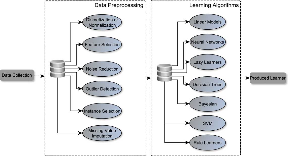
Figure 1 Predictive modeling process
One of the key challenges in the DM approach that is related to the performance of the learning algorithms, is the result to be dense and easily clarified. The representation of the dataset plays an important role in accomplishing this task. A dataset with too many features or features with correlations should not be included in the learning process, since these kinds of data does not offer useful information (Guyon & Elisseeff, Reference Guyon and Elisseeff2003). Thus, to use only the most informative data it is necessary to select features that will reduce information which is unnecessary and unrelated to the objective of our study. Furthermore, instance and feature selection (FS) is also useful in distributed DM and knowledge discovery from distributed databases (Skillicorn & McConnell, Reference Skillicorn and McConnell2008; Czarnowski, Reference Czarnowski2010).
An alternative approach towards the usage of informative data is the feature weighting approach based on some conditions (e.g., distance metrics) (Panday et al., Reference Panday, de Amorim and Lane2018; Zhou et al., Reference Zhou, Chen, Feng, Zhang, Shen and Zhou2018). To this end, the original dataset can be separated into weighted features and the features with the highest weight are involved in the learning process. In addition, in many cases it is more useful to construct features by transforming the initial dataset instead of finding a good subset of features (Mahanipour et al., Reference Mahanipour, Nezamabadi-pour and Nikpour2018; Virgolin et al., Reference Virgolin, Alderliesten, Bel, Witteveen and Bosman2018).
As we have already mentioned, the paper at hand addresses issues of data preprocessing. For more details about this subject, the reader is referred to Pyle (Reference Pyle1999) and García et al. (Reference García, Luengo and Herrera2015). In this article, we focus on the most well-known and widely used up-to-date algorithms for each step of data preprocessing in predictive DM.
The next section covers noise and outlier detection. The topic of processing unknown feature values is described in Section 3. Next, in Section 4 the normalization and discretization processes are presented. Sections 5 and 6 cover, respectively, instance and FS. The paper ends in Section 7 with a discussion and some concluding remarks. In addition, at the end of each section, we provide a table of citationsFootnote 1 that the most known and widely used methods of each data preprocessing step have received. In our point of view, this reveals the importance and the contribution of each method as well as its impact on the scientific community. Moreover, the reader can study a brief description of each method which is included in every table. Finally, the reader can reach in the Appendix a simple code of basic preprocessing steps, that gives simple tutorial examples in R programming language related to the usage of some known preprocessing algorithms.
2 Noise and outlier detection
One of the main problems to be tackled is that a variety of algorithms, such as instance-based learners, are sensitive to the presence of noise. This has the effect of misclassification which is based, for example, on the wrong nearest neighbor. This is so, because similarity measures can easily be falsified by data with noise in their values. A well-known preprocessing technique for finding and removing the noisy instances in the dataset is the noise filters. As a result, a new improved set of data is generated without noise and the resulting dataset can be used as input to a DM algorithm.
A simple filter approach is the variable-by-variable data cleaning. In this approach, the values that are considered as ‘suspicious’ values according to specific criteria are discarded or corrected. Thus, they can be included in the dataset that will be given as input to a DM algorithm. In this approach, the criteria include, among others, the following: an expert evaluates the suspicious data as errors or as false labeled or in other cases a classifier predicts those values as ‘unclear’ data.
As we have already mentioned in the introduction, besides the effect of noisy values, it is possible the appearance of dataset values called outliers. In Aggarwal (Reference Aggarwal2013) the author has described a method for creating a sorted list of values, with those values that are higher to be identified as outliers. Below in this section we describe methods used to identify outliers, as they are categorized in the following way (Chen et al., Reference Chen, Wang and van Zuylen2010a):
(a) statistics-based methods,
(b) distance-based methods,
(c) density-based methods.
A basic statistics-based method has been presented in Huang et al. (Reference Huang, Lin, Chen and Fan2006). It assumes a statistical model or a distribution (e.g., Gaussian or normal) for the original dataset and the outliers can be detected by using some statistical tests. In addition, many methods, like the technique that has been proposed in Buzzi-Ferraris and Manenti (Reference Buzzi-Ferraris and Manenti2011) identify the outliers and at the same time they evaluate the mean, the variance and those values that are outliers.
In the case of large datasets, in Angiulli and Pizzuti (Reference Angiulli and Pizzuti2005) the authors have proposed a distance-based outlier detection algorithm which is able to identify the top m outliers of the dataset, where m is a given integer. Their algorithm, called HilOut, computes the weight of a point as the sum of the distance separating it from its k-nearest neighbors (k-NN). Hence, the points with the highest amount of weight are identified as the outliers. A similar approach for the detection of mining distance-based outliers is related to the fast algorithm, called RBRP, that has been presented in Ghoting et al. (Reference Ghoting, Parthasarathy and Otey2008). Specifically, the authors faced the problem of outlier detection in high-dimensional datasets. The experiments that they conducted shown that their method is more efficient in terms of computational time, compared to other approaches. An outlier mining algorithm, named OMABD, which is based on dissimilarity has been proposed in Zhou and Chen (Reference Zhou and Chen2012). According to this algorithm, the detection of outliers is based on a comparison of two values: (i) the first value determines the dissimilarity degree that is constructed by the dissimilarity of each object of the dataset and (ii) the second one determines a dissimilarity threshold. In Filzmoser et al. (Reference Filzmoser, Maronna and Werner2008) the authors have proposed a more computationally efficient algorithm for detecting the outliers of a dataset. This algorithm is able to handle efficiently high-dimensional datasets using principal component analysis (PCA). Last but not least we refer to the method that has been proposed in Chen et al. (Reference Chen, Miao and Zhang2010b) which implements the neighborhood outlier identification. So, inspired from the well-known and widely used k-NN algorithm, the authors created a new algorithm called neighborhood based outlier detection algorithm. This algorithm compared with classic distance metric methods, such as k-NN, distance-based and replicator neural network based outlier detection method, outperformed the above methods in the case of the mixed datasets.
The density-based outlier detection identifies an outlying instance regarding the density of the surrounding space. Despite the fact that density-based outlier detection methods have an amount of advantages, the computational complexity issue remains a strong and of great concern problem for its application. An approach for the reduction of the computational complexity of density-based outlier detection has been proposed in Kim et al. (Reference Kim, Cho, Kang and Kang2011). Particularly, the authors combine two known techniques: the KD-tree structure and the k-NN algorithm, to improve the performance of the existing local outlier factor (LOF) algorithm. The experimental results that they have noted over three known datasets of UCI (University of California at Irvine Machine Learning Repository), shown that their approximation is better in terms of computational time than the original LOF algorithm.
On the other hand, in Liu et al. (Reference Liu, Ting and Zhou2012) the authors proposed an approach without using a density parameter. Their method, called iForest, was compared with several known methods, such as random forest, LOF, one class of SVM and ORCA. The experimental results showed that iForest overcomes all the above methods in terms of computational time and it needs more less memory-requirement than the other methods. Specifically, this method focuses randomly on a specific feature. It selects randomly a value between the maximum and minimum values of the specific feature to ‘isolate’ instances. This process can be iteratively repeated with the usage of a tree structure. The required number of partitions to apply the above isolation procedure to a dataset is the same as the length of the path from the top of the tree to the terminating node on its leaves. As they noticed, in such an itree, if a path length for specific instances is shorter than the expected, then they are highly likely to be anomalies. The editing techniques focus specifically on the removal of noise or anomalous instances in the training set (Segata et al., Reference Segata, Blanzieri, Delany and Cunningham2010). Therefore, the assessment of each individual instance of the dataset whether or not to be removed is necessary and very important. Approaches for the outlier detection and noise filtering can be categorized as (i) supervised, (ii) semi-supervised and (iii) unsupervised (Angiulli & Fassetti, Reference Angiulli and Fassetti2014). The supervised and semi-supervised methods, label data to create a model that unravels outliers from inliers. On the other hand, unsupervised approaches do not require any label object and detect outliers as points that are quite dissimilar from the remaining ones.
Another important issue which is related to noise is the case where the noise affects the output attribute. It is widely known that noise affects both input and output attributes. In Brodley & Friedl (Reference Brodley and Friedl1999) an ensemble filter (EF) which improves the filtering by the usage of a set of learners has been introduced. So, the authors conducted experiments included single classifiers and a set of classifiers, testing the EF over several datasets. The experimental results showed that the classification accuracy was better when the filtering approach of the multiple learners was used. In Delany et al. (Reference Delany, Segata and Mac Namee2012) the authors have presented a very useful study on the evaluation of different noise reduction techniques regarding the form of the examples on which the techniques are focused. The results that have been obtained in Sáez et al. (Reference Sáez, Luengo and Herrera2013) have shown that there is a notable relation between the complexity metrics of a dataset and the efficiency and effectiveness of several noise filters which are related to the nearest-neighbor classifiers.
In Sáez et al. (Reference Sáez, Galar, Luengo and Herrera2016) the authors have proposed a method that combines the decision of many classifiers to detect noise by unifying many different learners through an iterative scheme. Specifically, the filtering scheme that they have introduced identifies the noise by avoiding the detection of noisy instances at every new iteration of the process. Also, in Garcia et al. (Reference Garcia, de Carvalho and Lorena2016a) the authors have examined how label noise detection can be improved by using an ensemble of noise filtering schemes. In this approach, the authors tried to limit the noisy data to the final dataset, as well as to remove the useless data. So, by creating meta-features from corrupted datasets, they have provided a meta-learning model that predicts the noisy data over a new dataset.
Furthermore, in Ekambaram et al. (Reference Ekambaram, Fefilatyev, Shreve, Kramer, Hall, Goldgof and Kasturi2016) it has been shown that some basic principles used in SVMs have the particularity of capturing the mislabelled examples as support vectors. Due to the fact that there cannot be a single method that overcomes all the others in a specific noise identification task, the research that has been presented in Garcia et al. (Reference Garcia, Lorena, Matwin and de Carvalho2016b) is of great importance, since it presents a recommendation for the expected performance of specific filters that are used for particular tasks.
Table 1 exhibits a brief description of the most known and widely used methods, related to the noise and outlier detection issues and presents their applicability. Furthermore, it presents information about the citations that they have received.
Table 1 Brief description, applicability in noise and outlier detection and number of citations of the references related to the noise and outlier detection issues presented in Section 2
TC=number of the total citations; CpY=number of citations per year; k-NN=k-nearest neighbor.
3 Missing feature values
The problem of missing feature values related to (not necessarily) large sets of data is one of the main problems that has to be tackled during data preprocessing. Most of the datasets in real-world applications are datasets that contain incomplete information, that is, missing a small or a large part of the dataset. There are classifiers that exhibit robust behavior in datasets with missing values, such as naive Bayes, and therefore the final result of the decision is not affected by the missing values. On the other hand, there are classifiers, such as neural networks and k-NN, that require a careful handling of the incomplete information.
The above-described problem has been a major concern for the scientific community and significant progress has been made by many researchers in this field over the last years (Zhang et al., Reference Zhang, Zhang, Zhu, Qin and Zhang2008). However, there are important issues that require attention and raise questions that the experts are called upon to answer. The most important question is derived from the source of this ‘incompleteness’. More specifically, is the dataset incomplete because someone forgot these values or for some other reason they were lost? as well as, does a particular feature considered for some reason as unnecessary or unenforceable? whereas in fact these data are useful and necessary for a better prediction by the learner. In general, missing at random means that the tendency for a data point to be missing is not related to the missing data, but it is related to some of the observed data. In this case, it is safe to remove the data with missing values depending upon their occurrences. On the other hand, in the other case (missing not at random) by removing instances with missing values could produce a bias in the learning model. Thus, we could use imputation in this case, but this does not necessarily give better results (Zhang et al., Reference Zhang, Zhang, Zhu, Qin and Zhang2008).
There are several methods and techniques for handling missing data which can be chosen as follows (Jerez et al., Reference Jerez, Molina, Garca-Laencina, Alba, Ribelles, Martn and Franco2010; Cismondi et al., Reference Cismondi, Fialho, Vieira, Reti, Sousa and Finkelstein2013):
(a) Most common feature value of a categorical attribute: Fill in missing values with the value that appears most often in the given dataset.
(b) Concept most common feature value of a categorical attribute: Similarly to the above case, except that the missing values are filled by the values of the same class.
(c) Mean substitution of a numerical attribute: Fill in missing feature values with the feature’s mean value that is computed using the available values. Alternatively, instead of using the ‘general’ feature mean, it can be used the feature mean of the samples that belong to the same class.
(d) Regression method for a numerical attribute or classification methods for a categorical attribute: Develop a regression model for the numerical attribute case, fill in the blanks of the dataset by taking the decision-outcome of the model that is builded in using all the other known features as predictors. Similarly, develop the classification model for the categorical case (Honghai et al., Reference Honghai, Guoshun, Cheng, Bingru and Yumei2005; Silva-Ramírez et al., Reference Silva-Ramírez, Pino-Mejas, López-Coello and Cubiles-de-la Vega2011).
(e) Method of treating missing feature values as special values: In this case, the unknown elements of the dataset are considered as complete new values for the features that contain missing values.
Furthermore, we point out that in Farhangfar et al. (Reference Farhangfar, Kurgan and Dy2008) an inclusive experimental study has been performed which is based on imputation methods to tackle the missing value problem in 15 discrete datasets. Their experiments have shown that on average the imputation improves the subsequent classification. Various other algorithms have been designed to impute target missing values such as the k-NN variant algorithm, the shell neighbors imputation (SNI) algorithm (Zhang, Reference Zhang2011) and the random method for single imputation (Qin et al., Reference Qin, Zhang, Zhu, Zhang and Zhang2009). Regarding the approach of Zhang (Reference Zhang2011) the author proposed a variation of the k-NNI algorithm. In this case only two neighbors take part in the selection of the most neighboring from the missing data value. Specifically, the left and the right one. These points are calculated using the shell neighbor definition. This constitutes the main difference with the k-NNI algorithm which takes the k neighbors, where k is fixed. The experimental results over mixed datasets shown that the SNI algorithm overcomes the k-NNI algorithm with respect to classification and imputation accuracy. Concerning the approach of Qin et al. (Reference Qin, Zhang, Zhu, Zhang and Zhang2009), the authors through experiments that they conducted, compared the kernel-based method that they proposed with several non-parametric methods. The results showed that their non-parametrical optimization (POP) algorithm outperforms the other methods regarding statistical parameters, such as mean, distribution function and quantile after missing data and imputation efficiency.
An imputation approach named NIIA has been proposed in Zhang et al. (Reference Zhang, Jin and Zhu2011). This method imputes missing data by using information within incomplete instances. It is an iterative imputation scheme that has been designed for imputing iteratively the missing target values. It imputes each missing value successively until its convergence.
In Luengo et al. (Reference Luengo, Garca and Herrera2012), the authors have tried to solve the missing value problem through the usage of different imputation methods. Specifically, they have focused on a classification task and their experimental results have shown that specific missing values imputation methods provide better results regarding the accuracy.
In Lobato et al. (Reference Lobato, Sales, Araujo, Tadaiesky, Dias, Ramos and Santana2015), the authors have presented for the first time a solution to the problem of missing values by combining evolutionary computation techniques, such as genetic algorithms (GA), for data imputation. In particular, the authors have proposed a multi-objective GA, named MOGAImp, which is suitable for mixed-attribute datasets.
A very difficult and time-consuming problem constitutes the selection of the optimal combination between classification and imputation methods. A new, alternative scheme that proposes such a combination adaptively has been introduced in Sim et al. (Reference Sim, Kwon and Lee2016). To build this new scheme and to find the proper pair among the imputation method and the classifier, the authors conducted a set of testing experiments. An important difference concerning the past attempts was that the authors used meta-data to cover missing data. Thus, they avoid the extremely high amount of executing time. In addition, another approach that covers the incomplete data through adaptive imputation based on belief function theory has been presented in Liu et al. (Reference Liu, Pan, Dezert and Martin2016). Specifically, the authors handle the problem of classification of incomplete patterns covering the missing values through the k-NN and self-organizing map methods. This occurs only in the cases where the available information are not enough for the classification of a given object.
Table 2 exhibits a brief description and information about the citations that the most known and widely used methods, related to the missing feature values issues, have received.
Table 2 Brief description and number of citations of the references related to the missing feature values issues presented in Section 3
TC=number of the total citations; CpY=number of citations per year; SVM=support vector machine; ANN=artificial neural network; k-NN=k-nearest neighbor.
4 Normalization and discretization
In various datasets that we have to manage, there are very often large differences between the feature values, such as the maximum and minimum value, for example, 0.001 and 10 000. In general, this issue is not desirable and requires careful intervention to make a scaling down transformation in such a way that all attribute values to be appropriate and acceptable. This process is known as feature scaling or data normalization (in the case of data preprocessing) and it is necessary and very important for various classifiers, such as neural networks, SVMs, k-NN algorithms, as well as fuzzy classifiers which cannot perform well if large differences between the feature values occur in the dataset.
The most common methods for this scope are the following:
(a) min–max normalization or feature scaling in [0, 1]. The formula that gives the new feature value is the following:
 $$v'{\equals}{{v{\minus}\min \_{\rm value}} \over {\max \_{\rm value}{\minus}\min \_{\rm value}}}$$
(b) min–max normalization or feature scaling in [a, b]. The formula that gives the new feature value is the following:
$$v'{\equals}{{v{\minus}\min \_{\rm value}} \over {\max \_{\rm value}{\minus}\min \_{\rm value}}}({\rm new}\max \_{\rm value}{\minus}{\rm new}\min \_{\rm value}){\plus}{\rm new}\min \_{\rm value}$$
(c) z-score normalization or standardization. The formula that gives the new standardization feature value is the following:
$$v'{\equals}{{v{\minus}{\rm mean}} \over {{\rm stand}\_{\rm dev}}}$$
(d) unit length scaling:


 $$v'{\equals}{v \over {{\rm P}\,v\,{\rm P}}}$$
where ‘v’ is the original feature value while ‘
 $$v'$$
’ is the new, normalized data value, ‘
$$v'$$
’ is the new, normalized data value, ‘
 $$\min \_\rm value$$
’ and ‘
$$\min \_\rm value$$
’ and ‘
 $$\max \_\rm value$$
’ are, respectively, the minimum and maximum feature values before the normalization process. In the second method, the interval [a, b] indicates a specific range that we want to transform into the original dataset. So, ‘
$$\max \_\rm value$$
’ are, respectively, the minimum and maximum feature values before the normalization process. In the second method, the interval [a, b] indicates a specific range that we want to transform into the original dataset. So, ‘
 $$\rm new\,\max \_value$$
’ and ‘
$$\rm new\,\max \_value$$
’ and ‘
 $$\rm new\,\min \_value$$
’ point out the desirable new maximum and new minimum value of the normalized dataset (the a and b value, respectively). Moreover, in method (c) ‘
$$\rm new\,\min \_value$$
’ point out the desirable new maximum and new minimum value of the normalized dataset (the a and b value, respectively). Moreover, in method (c) ‘
 $${\rm mean}$$
’ denotes the mean value of the feature vector and ‘
$${\rm mean}$$
’ denotes the mean value of the feature vector and ‘
 $${\rm stand}\_{\rm dev}$$
’ represents the standard deviation. Essentially, this method constitutes a measurement of how many standard deviations the value is from its mean value. Finally, the ‘
$${\rm stand}\_{\rm dev}$$
’ represents the standard deviation. Essentially, this method constitutes a measurement of how many standard deviations the value is from its mean value. Finally, the ‘
 $${\rm P} \cdot {\rm P}$$
’ indicates a norm, for example, the Euclidian length of the feature vector or the Manhattan distance. In conclusion, selecting one of the above normalization methods is clearly dependent on the dataset we want to normalize (or transform).
$${\rm P} \cdot {\rm P}$$
’ indicates a norm, for example, the Euclidian length of the feature vector or the Manhattan distance. In conclusion, selecting one of the above normalization methods is clearly dependent on the dataset we want to normalize (or transform).
Another important issue to address is that of values of the continuous features of a dataset. Usually, the features of the sample can get continuous values or values from a wide range. This may require a time-consuming procedure to handle or, in many cases, may be inefficient for the processes used in the field of predictive DM. Thus, the main outcome of these and a solution to the above problem is the discretization process.
The discretization process can actually be very useful to a variety of classifiers, such as decision trees (DTs) or Bayesian classifiers. On the other hand, the scientific community needs to resolve several other issues about this process, as identifying the most appropriate interval borders or the right arity for the discretization of a numerical value range. These issues are open to resolution and extensive study. For more details about the discretization processes, the reader is referred to Liu et al. (Reference Liu, Hussain, Tan and Dash2002), Kurgan and Cios (Reference Kurgan and Cios2004) and Liu and Wang (Reference Liu and Wang2005).
The main difference between supervised and unsupervised discretization methods is that the methods of the first category discretize the features of the dataset regarding the class in which they belong, while the other ones do not. On the other hand, the distinction of methods in top-down and bottom-up methods concerns the initialization of the starting interval. In the top-down methods, the initialization takes place to the starting interval and retrospectively cleaved into smaller ones. On the other hand, in the bottom-up methods the initialization of single value intervals takes place followed by merging of adjacent intervals. Moreover, the quality of the discretization processes is measured using two basic criteria: (i) the classification performance and (ii) the number of discretization intervals.
Two of the most well-known and widely used discretization methods are (Dougherty et al., Reference Dougherty, Kohavi and Sahami1995): (i) the equal size and (ii) the equal frequency. Both of them are unsupervised methods. The first method, as its name implies, finds the maximum and the minimum value of the attributes, and then divides the found range into k equal-sized intervals. The second one finds the number of values of the attribute and then it separates them into intervals which contain the same number of instances.
A very important issue regarding the top-down and the bottom-up methods is that they require the involvement of the user with respect to a set of parameters, such as the modification of the criteria for stopping the discretization processes. A well-known bottom-up discretization algorithm, named Khiops has been presented in Boulle (Reference Boulle2004). The advantage of this method with respect to the other methods of the same category, and especially the ChiSplit and the ChiMerge, is that it uses as stopping criterion the χ 2 statistical test. As a result, this method optimizes a global criterion and not a local one. Moreover, it does not require any parameters to be specified by the user. Furthermore, it is not lagging in terms of time complexity (as it is demonstrated by the experimental results) in accordance with other methods that optimize a local criterion. This makes Khiops a very useful and easy to be handled. Another well-known method of the same family, called Ameva, manages to potentially produce the minimum number of intervals, has been presented in Gonzalez-Abril et al. (Reference Gonzalez-Abril, Cuberos, Velasco and Ortega2009). Specifically, this method has been compared with the known algorithm, called CAIM and also with other genetic approaches. The experimental results have shown that the Ameva always produces the smallest number of discrete intervals and even, in cases with a large number of classes is not lagging in terms of complexity. Regarding the performance of Ameva in relation with the genetic approaches, the performance of these algorithms is very similar.
In Tsai et al. (Reference Tsai, Lee and Yang2008), the authors have proposed an incremental, supervised and top-down discretization algorithm through which better classification accuracy has been achieved. This algorithm is based on the class-attribute contingency coefficient and it is combined with a greedy method that has also exhibited good execution time results. As we have already mentioned, the measurement of the quality of the discretization algorithms is one of the issues that deserves a thorough attention. The experiments that have been carried out in Jin et al. (Reference Jin, Breitbart and Muoh2009) have shown that more discretized intervals usually equate to fewer classification errors and as a result lower the cost of the data discretization process.
In Janssens et al. (Reference Janssens, Brijs, Vanhoof and Wets2006) the concepts of (i) error-based, (ii) entropy-based and (iii) cost-based discretization methods have been analyzed. The methods of the first category, group the values into one interval aiming through the minimization of the errors in the training set to achieve the optimal discretization. On the other hand, entropy-based methods, use the entropy value of a point to find the min–max value of an interval. Like top-down methods, the entropy discritization methods, divide the starting interval into smaller ones by choosing the values which minimize the entropy until the intervals become optimal or some specific criteria to be fulfilled (Kumar & Zhang, Reference Kumar and Zhang2007). This category is widely used and the notion of entropy has been used also in Gupta et al. (Reference Gupta, Mehrotra and Mohan2010) and de Sá et al. (Reference de Sá, Soares and Knobbe2016) to exploit the inter-attribute dependencies of the data as well as to discretize the rank of data. On the other hand, with the error-based methods of the third category, the error is taken into account as a cost of misclassification.
The Bayesian classifiers are among the most known classifiers in DM, and therefore the researchers have been highly involved in this category of algorithms. Specifically, to improve the rate of accuracy in the prediction of naive Bayes classifier, in particular in reducing the variance and the bias, in Yang et al. (Reference Yang, Webb and Wu2009) it has been proposed a scheme that combines proportional discretization and fixed frequency discretization. Another attempt to improve the accuracy of naive Bayes classifier has been done in Wong (Reference Wong2012). The author, in his attempt to present a relationship that would explain the level of dependence between the class and the continuous feature, has proposed a method which uses a non-parametric measure. With this measure the author eventually has achieved the improvement of the classifier. Furthermore, through the extensive experimental research that it has been carried out in Mizianty et al. (Reference Mizianty, Kurgan and Ogiela2010), an important observation regarding the discretization process and its effect on both naive and semi-naive Bayesian classifiers has been obtained. The authors have shown that despite the time-consuming process of discretization relative to training time of classifier, the whole process often is completed faster than naive Bayes classification process.
A method that performs the discretization process automatically, based on two factors: (i) the dispersion as well as (ii) the uncertainty of the range of the data has been presented in Augasta & Kathirvalavakumar (Reference Augasta and Kathirvalavakumar2012). The experiments conducted by the authors that are based on real-world data have shown that the proposed algorithm approaches to give the smallest number of discrete intervals, and the discretization time is less than other algorithms. In addition, in Li et al. (Reference Li, Deng, Feng and Fan2011) the authors have proposed the class-attribute coherence maximization (CACM) criterion and the corresponding discretization algorithms: (i) the CACM algorithm and (ii) the efficient-CACM algorithm. The extensive experiments they have done show that their method surpasses the performance of other well-known classifiers such as RBF-SVM and C4.5. In addition, the variation that they gave was faster compared with the fast-CAIM method.
Furthermore, in Cano et al. (Reference Cano, Nguyen, Ventura and Cios2016) an improved version of the CAIM algorithm has been proposed. The new algorithm, named ur-CAIM achieves more flexible discretization, it presents more qualitative subintervals and it has better classification results for unbalanced data. In addition, a more complete and more detailed survey about discretization methods has been presented in Yang et al. (Reference Yang, Webb and Wu2009), as well as a taxonomy and empirical analysis of these methods has been presented in Garcia et al. (Reference García, Luengo, Sáez, Lopez and Herrera2013). Also, an updated overview of discretization techniques in conjunction with taxonomy has been presented in Ramírez-Gallego et al. (Reference Ramírez-Gallego, Garca, Mouriño-Taln, Martnez-Rego, Bolón-Canedo, Alonso-Betanzos, Bentez and Herrera2016).
Table 3 exhibits a brief description and information about the citations that the most known and widely used methods, related to the normalization and discretization issues, have received.
Table 3 Brief description and number of citations of the references related to the normalization and discretization issues presented in Section 4
TC=number of the total citations; CpY=number of citations per year.
5 Instance selection
The instance selection approach is not only used to handle noise (Aridas et al., Reference Aridas, Kotsiantis and Vrahatis2016; Aridas et al., Reference Aridas, Kotsiantis and Vrahatis2017) but also to deal with the infeasibility of learning from huge datasets (Wu & Zhu, Reference Wu and Zhu2008). The training time required by the neural networks and SVMs as well as the classification time of instance-based learners is clearly affected by the size of the dataset. In this case, instance selection can be considered as an optimization problem that attempts to maintain the quality along with minimizing the size of the dataset (Liu & Motoda, Reference Liu and Motoda2002). Moreover, by increasing the number of instances the complexity of the induced model is risen resulting to the decrease of the interpretability of the results. Thus, instance selection is highly recommended in the case of big datasets as it is noted in García-Pedrajas and PéRez-RodríGuez (Reference GarcíA-Pedrajas and PéRez-RodríGuez2012).
The sampling is a widely used process since it constitutes a powerful computationally intense procedure operating on a sub-sample of the dataset and is able to maintain or even to increase the accuracy (Klinkenberg, Reference Klinkenberg2004). There is a variety of procedures for sampling instances from a large dataset (over a Gb). The most well-known are the following (Cano et al., Reference Cano, Herrera and Lozano2005): (i) the random sampling that selects a subset of instances randomly and (ii) the stratified sampling in the case where the class values are not uniformly distributed in the dataset.
In Reinartz (Reference Reinartz2002), the author has presented a unifying framework, which covers approaches related to instance selection. Furthermore, in Kim and Oommen (Reference Kim and Oommen2003) and in García et al. (Reference García, Derrac, Cano and Herrera2012a) a taxonomy and a ranking of prototype reduction schemes have been also provided. In general, instance selection methods have been grouped into different categories according to Olvera-López et al. (Reference Olvera-López, Carrasco-Ochoa, Martnez-Trinidad and Kittler2010):
(a) Type of selection: (i) The condensation methods that try to compute a consistent subset by removing instances that cannot increase the classification accuracy, (ii) the edition methods that try to remove noisy instances and (iii) the hybrid methods that search for a subset in which both noisy and useless instances occur.
(b) Direction of search: (i) The incremental methods that start with an empty set and add instances according to some criterion, on the contrary (ii) the decremental methods that start with the whole set and remove instances according to some criterion and (iii) the mixed methods that start with a subset and add or remove instances that fulfill a certain criterion.
(c) Evaluation of search: (i) The wrapper methods that consider a selection criterion based on the accuracy obtained by a classifier and (ii) the filter methods that use a selection function that is not based on a specific classifier.
In Bezdek and Kuncheva (Reference Bezdek and Kuncheva2001), the authors have compared 11 methods for finding prototypes upon which the nearest-neighbor classifier is based. In this comparison, several methods have exhibited a good performance and none of them is superior to all the others. In the case of binary problems, an important observation has been presented in Pkekalska et al. (Reference Pkekalska, Duin and Paclk2006). Specifically, according to their observation the dissimilarity-based discrimination functions relying on reduced prototype sets (3–10% of the training instances) offer a similar or much better classification accuracy than the k-NN applied on the entire training set. Also, the selection rule is related to the k-NN classifier in most wrapper algorithms (Derrac et al., Reference Derrac, Garca and Herrera2010b).
A well-known algorithm for instance selection is the HitMiss network (HMN) algorithm that it has been proposed in Marchiori (Reference Marchiori2008). This algorithm focuses on the redundancy removal rather than the noise reduction. Specifically, the proposed algorithm was used to improve the performance of the 1-NN algorithm. The author proposed three variants of the original algorithm. Each of them provided separate advantages and improvements with respect to the 1-NN algorithm. For example, the variant called HMN-C deleted instances from the dataset but nevertheless it did not affect the accuracy of the 1-NN algorithm. Or the HMN-EI version that it repeatedly ran the HMN-E version, which was the second one that made storage reduction. All the three variants were tested extensively on multiple, diverse datasets. The results showed that the proposed algorithm has a better generalization ability than other known instance selection algorithms. In addition, it greatly improves the accuracy of the 1-NN classifier. Furthermore, in Nikolaidis et al. (Reference Nikolaidis, Goulermas and Wu2011), the authors have proposed the class boundary preserving algorithm. This approach uses the concept of reachable set and proposes an extension involving more than just the nearest enemy. Then, by using the multiple reachable sets and the nearest enemies establishes geometric structure patterns to remove redundant instances.
In de Haro-García & García-Pedrajas (Reference de Haro-García and García-Pedrajas2009) an instance selection filtering strategy has been proposed. In this strategy, the main idea is to divide the dataset into small mutually exclusive blocks and then individually to apply an instance selection algorithm to each block. Afterward, the instances that are selected from each block are merged in subsets of about the same size and the instance selection algorithm is applied again. The process is repeated until a validation error starts to increase.
In Czarnowski (Reference Czarnowski2012) a clustering approach for instance selection has been presented. Initially, this approach makes groups of instances of each class into clusters and then, in the second step a wrapper process is used. Furthermore, an evolutionary instance selection algorithm has been proposed in García et al. (Reference García, Cano and Herrera2008). Specifically, this algorithm uses a memetic algorithm that combines evolutionary algorithms and local search strategies. Due to this combination, the inherent convergence problem is avoided that plagues evolutionary algorithms. In fact, very good results are achieved as the number of data increases. An additional evolutionary instance selection algorithm is the cooperative coevolutionary instance selection algorithm that has been proposed in García-Pedrajas et al. (Reference García-Pedrajas, Del Castillo and Ortiz-Boyer2010). In this approach, the technique of divide and conquer is utilized. Thus, the original dataset is subdivided into smaller ones, and a global optimization technique, based on populations, is looking for the best combination. The advantage of this method is that the user can control the objective functions (such as accuracy or storage requirements) through the fitness function. In addition, this approach does not require the calculation of a distance metric or the usage of a particular classification algorithm. The experimental results have shown that the proposed algorithm is not inferior to any other of the compared algorithms. In addition, it is superior in requirement terms and it is promising in the case of large datasets regarding to the terms of computational cost and efficiency.
For the characterization of datasets various measures have been proposed in Caises et al. (Reference Caises, González, Leyva and Pérez2011). These measures are used to select from some pre-selected methods, the method (or combination of methods) that is expected to produce the best results. Furthermore, an instance ranking method per class using borders has been introduced in Hernandez-Leal et al. (Reference Hernandez-Leal, Carrasco-Ochoa, Martnez-Trinidad and Olvera-Lopez2013). The border instances are those nearby to the decision boundaries between the classes and are the most useful for the learning algorithms.
In Lin et al. (Reference Lin, Tsai, Ke, Hung and Eberle2015), the authors have introduced the representative data detection approach, which is based on outlier pattern analysis and prediction. A learning model is initially trained to learn the patterns of (un)representative data that are selected by a specific instance selection method from a small amount of training data. Afterwards, the leaner can be used to select the rest useful instances of the large amount of training data.
In Arnaiz-González et al. (Reference Arnaiz-González, Dez-Pastor, RodríGuez and Garca-Osorio2016), two new algorithms with linear complexity for instance selection purposes have been presented. Both algorithms use locality-sensitive hashing to find similarities between instances. Also, in Tsai and Chang (Reference Tsai and Chang2016), the authors have investigated the effect of performing instance selection to filter out some noisy data regarding the imputation task. In particular, the authors have examined whether the instance selection process should precede or follow the imputation process. For this purpose, they have provided four ways/combinations to find which one is the best. This has the effect of identifying/creating the most appropriate training set for the classifier that used. The authors have performed extensive experiments to find the best combination on a variety of datasets. The four combinations have been tested for the k-NN and SVM classifier.
In Liu et al. (Reference Liu, Wang, Wang, Lv and Konan2017), the authors have studied the support vector recognition problem mainly in the context of the reduction methods to reconstruct the training set. The authors have focused on the fact of uneven distribution of instances in the vector space to propose an efficient self-adaption instance selection algorithm from the viewpoint of geometry-based method.
Furthermore, recently, in Fernández et al. (Reference Fernández, Carmona, del Jesus and Herrera2017) the authors have used a multi-objective evolutionary algorithm to obtain an optimal joint set of both features and instances. Specifically, the proposed methodology has been applied to imbalanced datasets. Using the well-known C4.5 classifier combined with the well-known NSGA-II evolutionary method, they were able to expand the search space, which enables to build an ensemble of classifiers. Thus, through FS overcomes the overlapping problem that is inherent in multi-class imbalanced datasets as well as through the instance selection two problems have been solved, namely the elimination of noise and the imbalance issue. The authors have conducted experiments including comparisons with widely used and well-known classifiers on binary-class and multi-class imbalanced datasets. The experimental results have shown that the proposed method named EFIS-MOEA exhibits a better performance than the compared ones and is promising in terms of its applicability to big datasets.
In general, the prototype generation (PG) approach builds new artificial prototypes to increase the accuracy. In Triguero et al. (Reference Triguero, Derrac, Garcia and Herrera2012b), the authors have provided a survey of PG methods that are specifically designed for the nearest-neighbor algorithm. Furthermore, they have conducted an experimental study to measure the performance in terms of accuracy and reduction capabilities.
In Nanni and Lumini (Reference Nanni and Lumini2011), instance generation for creating an ensemble of the classifiers has been used. The training phase consists in repeating N times the PG, and then the scores resulting from classifying a test instance using each set of prototypes are combined by voting.
In general, the classifiers are expected to be able to generalize over unseen instances of any class with equal accuracy, which constitutes an ideal situation. Also, in many applications learners are faced with imbalanced datasets, which can cause the learner to be biased towards one class. This bias is the result of one class being greatly under-represented in the training data compared to the other classes. It is related to the way in which learners are designed. Inductive learners are typically designed to minimize errors over the training examples. Classes that contain few examples can be mostly ignored by learning algorithms since the cost of performing well on the over-represented class outweighs the cost of doing poorly on the smaller class (He & Garcia, Reference He and Garcia2009).
We point out that the imbalanced datasets have recently received attention in various ML tasks (Lemaître et al., Reference Lemaître, Nogueira and Aridas2017). There are various procedures to cope with the imbalanced problem in datasets include among others the following (Sun et al., Reference Sun, Wong and Kamel2009): (i) duplicate training examples of the under-represented class which is actually re-sampling the examples (over-sampling), (ii) remove training examples of the over-represented class which is referred to as downsizing (under-sampling), (iii) combine of both over- and under-sampling and (iv) ensemble learning approaches.
In Chawla et al. (Reference Chawla, Bowyer, Hall and Kegelmeyer2002), the authors have proposed the synthetic minority over-sampling technique (SMOTE) where synthetic (artificial) samples are generated rather than over-sampling. SMOTE generates the same number of synthetic data samples for each original minority instance. This happens without consideration to neighboring examples, which increases the occurrence of overlapping between classes (Wang & Japkowicz, Reference Wang and Japkowicz2004).
In Farquad and Bose (Reference Farquad and Bose2012), the authors have employed SVM as a preprocessor. Their approach replaces the actual target values of the training data by the predictions of the trained SVM. Next, the modified training data are used to train other learners.
In van Hulse and Khoshgoftaar (Reference van Hulse and Khoshgoftaar2009), a comprehensive experimental investigation using noisy and imbalanced data has been presented. The results of the experiments demonstrate the impacts of the noise on learning from imbalanced data. Specifically, the noise resulting from the corruption of instances from the true minority class is seems to be the most severe. In Cano et al. (Reference Cano, Garca and Herrera2008), the authors have proposed the combination of the stratification and the instance selection algorithms for scaling down the dataset. Two stratification models have used to increase the presence of minority classes in datasets before the instance selection.
As we have already mentioned in the introduction and as it is noted in the literature (López et al., Reference López, Fernández, Moreno-Torres and Herrera2012), the problem of managing imbalanced datasets is one of the most important and most difficult problems in DM. The classification problem is a widely encountered problem with so many aspects. The most common approaches include: data sampling or appropriate modification of the algorithm to be able to handle imbalanced datasets. According to the authors of López et al. (Reference López, Fernández, Moreno-Torres and Herrera2012), the solution seeks to the suitable combination of the above approaches. In particular, they have observed that learning solutions which are cost-sensitive if they combined with data sampling and algorithmic modification, can reach better misclassification costs in the minority class. In addition, they have minimized the high-cost errors.
Experiments over 17 real datasets using eight different classifiers have shown that over-sampling the minority class outperforms under-sampling the majority class when the datasets are strongly imbalanced. On the other hand, there are not significant differences for the databases with a low imbalance (García et al. Reference García, Sánchez and Mollineda2012a).
Table 4 exhibits a brief description and information about the citations that the most known and widely used methods, related to the instance selection issues, have received.
Table 4 Brief description and number of citations of the references related to the instance selection issues presented in Section 5
TC=number of the total citations; CpY=number of citations per year.
6 Feature selection
It is well-known and widely recognized that several learners, such as the k-NN procedure, is very sensitive relative to irrelevant features. In addition, the presence of irrelevant features can make SVMs and neural network training very inefficient and in many cases impractical. Furthermore, the Bayesian classifiers do not perform well in the case of redundant variables. To tackle these issues, the FS approach is proposed to be used. The FS is the procedure of identifying and removing as many irrelevant and redundant features as possible. This reduces the dimensionality of the data and facilitates learning algorithms to operate faster and more effectively. In general, the features can be distinguished as follows (Hua et al., Reference Hua, Xiong, Lowey, Suh and Dougherty2005):
(a) Relevant: The features that have an influence on the class and their role cannot be assumed by the rest.
(b) Irrelevant: Irrelevant features that do not have any influence on the class.
(c) Redundant: A redundancy occurs whenever a feature can take the role of another (perhaps the simplest way to model redundancy). In practice, it is not so straightforward to determine feature redundancy when a feature is correlated (perhaps partially) with a set of features.
In general, the FS algorithms consist of two approaches (Hua et al., Reference Hua, Xiong, Lowey, Suh and Dougherty2005): (i) a selection algorithm that generates the proposed subsets of features to find an optimal subset and (ii) an evolutionary algorithm that decides about the quality of the proposed feature subset by returning some ‘measure of goodness’ to the selection algorithm. On the other hand, without the application of a proper stopping criterion, it is possible the FS process to run in an exhaustively way or without termination through the space of subsets. Usually, the stopping criteria are: (i) either the addition (or the deletion) of any feature that does not offer a better subset and/or (ii) whether an optimal subset has been found according to some evaluation function. In Piramuthu (Reference Piramuthu2004), various FS techniques have been compared concluding that none of them is superior to all the others.
Regarding the selection strategy, the filtering methods rank features independently of the classifier. In the filtering methods, a feature can be selected by taking into consideration some predefined criteria such as: (i) mutual information (Chow & Huang, Reference Chow and Huang2005), (ii) class separability measure (Mao, Reference Mao2004) or (iii) variable ranking (Caruana & Sa, Reference Caruana and de Sa2003).
On the other hand, the wrapper methods use a classifier to assess feature subsets. These methods are computationally consuming in practice and they are not independent of the type of classifier used (Liu & Motoda, Reference Liu and Motoda2007). The wrapper methods use the cross-validation approach to predict the benefits of adding or removing a feature from the feature subset used. In the case of the forward stepwise selection, a feature subset is iteratively build up. Each of the unused features is added to the model in turn, and the feature that most improves the accuracy of the model is chosen. In the case of the backward stepwise selection, the algorithm starts by building a model that includes all the available input features. In each iteration, the algorithm locates the variable whose its absence causes the most improvement of the performance (or causes least deterioration). A problem with the forward selection is that it may fail to include features that are interdependent since it adds one variable at a time. On the other hand, it is able to locate small effective subsets quite soon, since the early evaluations that involve relatively few features are fast. On the contrary, in the backward selection interdependencies are well handled, but at the beginning the evaluations are computationally consuming.
Various FS methods treat the multi-class case directly rather than decomposing it into several two-class problems. The sequential forward floating selection and the sequential backward floating selection are characterized by the changing number of features that are included or are eliminated at different stages of the procedure (Somol & Pudil, Reference Somol and Pudil2002). In Maldonado and Weber (Reference Maldonado and Weber2009), the authors have introduced a wrapper algorithm for FS by using SVMs with kernel functions. Their method is based on a sequential backward selection by using the number of misclassifications in a validation subset as the measure to decide which feature has to be eliminated in each step.
Furthermore, the GA is an additional well-known approach to tackle FS issues (Smith & Bull, Reference Smith and Bull2005). In this approach, for each iteration a feature is chosen and it is decided whether to be included in the subset or to be excluded from it. All the combinations of unknown features are used with an equal probability. Due to the probabilistic nature of the search, a feature that should be in the subset will be superior of the others, even whether it is dependent on another feature. An important characteristic of the GA is that it is designed to exploit the epistasis (that is the interdependency between bits in the string), and thus is well-suited for the FS approach. On the other hand, GAs typically require a large number of evaluations to reach a minimizer.
To combine the advantages of the filter and the wrapper models, various hybrid models have been proposed to deal with high-dimensional data. In Unler et al. (Reference Unler, Murat and Chinnam2011), the authors have presented a hybrid filter-wrapper feature subset selection algorithm which is based on the particle swarm optimization (PSO) (Kennedy & Eberhart, Reference Kennedy and Eberhart1995; Parsopoulos & Vrahatis, Reference Parsopoulos and Vrahatis2010) for the SVM classification. The filter model is based on the mutual information and is a combined measure of feature relevance and redundancy with respect to the selected feature subset. Also, the wrapper model can be considered as a modified discrete PSO algorithm.
In Hu et al. (Reference Hu, Che, Zhang and Yu2010), the authors have proposed a concept of neighborhood margin and neighborhood soft margin to calculate the minimal distance between different classes. They have used the criterion of the neighborhood soft margin to estimate the quality of the candidate features and to build a forward greedy algorithm for FS.
Instead of approaching instance selection or FS problems separately, various research efforts have been made for the study of the simultaneous instance selection and FS (Derrac et al., Reference Derrac, Garca and Herrera2010a). To make this happen, the authors provided an evolutionary scheme that applied to the k-NN classification problem. The experimental results showed that the proposed method outperforms other well-known evolutionary approaches, such as FS-GGA, FS-SSGA, FS-CHC and 1-NN, regarding the data reduction process.
Furthermore, in Shu and Shen (Reference Shu and Shen2016), the authors, based on the rough set theory, have addressed the problem of the FS for cost-sensitive data with missing values. They have proposed a multicriteria evaluation function to characterize the significance of the candidate features. In particular, this occurs by taking into consideration not only the power in the positive region and boundary region but also their associated costs.
In general, in the FS approaches, a feature takes a binary weight, where ‘1’ indicates that the feature has been selected and ‘0’ otherwise. However, feature weighting assigns a value, usually in the interval [0, 1] to each feature and the greater this value is, the more salient the feature will be. The usage of the weight-based models is widely used in various classification issues (Wettschereck et al., Reference Wettschereck, Aha and Mohri1997). In general, for this usage, the weighted neural networks can be considered as the most used example (Park, Reference Park2009), while, SVMs (Shen et al., Reference Shen, Wang and Yu2012) and nearest-neighbor methods (Mateos-García et al., Reference Mateos-García, García-Gutiérrez and Riquelme-Santos2012) can also use weights for a better performance. Also, it is well known that the proper adjustment of the weights during the training process improves the model classification accuracy. In Triguero et al. (Reference Triguero, Derrac, Garcia and Herrera2012a), the authors have incorporated a new feature weighting scheme using two different prototype generation methodologies. In essence, the authors with the proposed hybrid evolutionary scheme improved the performance of other evolutionary approaches that have been used to optimizing the positions of the prototypes.
It is widely known that the DTs use the divide and conquer procedure, thus, they tend to perform well whether a few very relevant attributes exist, but less in the case where many complicate interactions exist. In general, the problem of the feature interaction can be tackled by constructing new features from the basic feature set. This procedure is called feature construction/transformation. In this case, the new generated features may lead to the creation of more concise and accurate classifiers. In addition, the discovery of meaningful features contributes to the improved comprehensibility of the produced classifier and the enhanced understanding of the learned concept.
In Smith and Bull (Reference Smith and Bull2005), the authors have used the approaches of the genetic programming and the GA as preprocessors of the dataset in the DTs. Specifically, for this case they have considered the C4.5 algorithm which is used to generate a DT. They have used the genetic programming as feature constructor and the GA as feature selector. Moreover, they have shown, by using 10 datasets that their framework performs better than the DTs alone. In addition, they have shown that effective preprocessing of the input data to DTs can significantly improve classification performance.
In general, PCA is a kind of analytical procedure based on a subspace and is able to estimate an original sample by using low-dimensional characteristic vectors (Hoffmann, Reference Hoffmann2007). Also, a large feature space can be converted to a low-dimensional one by training a multilayer neural network with small hidden layers. Thus, the well-known and widely used gradient descent optimization methods can then be used for fine-tuning the weights in such autoencoder networks (Hinton & Salakhutdinov, Reference Hinton and Salakhutdinov2006). Hence, while PCA is restricted to a linear map, the autoencoders do not.
It has been shown that feature construction reduces the complexity of the space spanned by the input data. In Piramuthu and Sikora (Reference Piramuthu and Sikora2009), the authors have presented an iterative algorithm for improving the performance of any inductive learning process by using the feature construction as a preprocessing step. The choice between FS and feature construction depends on the application domain and the specific available training set. In general, FS leads to savings in measurements cost since some of the features are discarded and the selected features retain their original physical interpretation. In addition, the retained features may be important for understanding the physical process that produces the patterns. On the contrast, transformed features generated by feature construction are able to provide a better discriminative ability than the best subset of the given features. On the other hand, these new features may not have a clear physical meaning.
Table 5 exhibits a brief description and information about the citations that the most known and widely used methods, related to the FS issues, have received.
Table 5 Brief description and number of citations of the references related to the feature selection issues presented in Section 6
TC=number of the total citations; CpY=number of citations per year; PCA=principal component analysis; PSO=particle swarm optimization; SVM=support vector machine.
7 Discussion and concluding remarks
Predictive DM algorithms enable us to discover knowledge from large datasets subjected to appropriate conditions. The most important issue is the original dataset to be reliable. If the data that are received as input by the DM algorithms are unreliable or are contaminated by noise, then they cannot provide good and competitive results. In other words, the datasets should be of a high quality to obtain reliable models that will provide accurate results. For these reasons, data preprocessing is necessary to exploit predictive DM algorithms in knowledge discovery processes.
Since the quality of the dataset and the performance of the DM algorithms are directly related, considerable efforts have been conducted by several researchers to record some seeking points regarding the influence of each other. Therefore, through experimental research that have been conducted by Crone et al. (Reference Crone, Lessmann and Stahlbock2006), it has been shown that the representation of the dataset affects quite a lot the learning methods and that the algorithm performance is better if efficient data preprocessing has been performed. In addition, the influence of preprocessing varies according to the algorithm. Thus, in the paper at hand the most well-known and widely used up-to-date algorithms for each step of the data preprocessing have been presented.
In the case where a dataset is huge, it may not be feasible to run a DM algorithm. To this end, it is necessary to reduce the amount of data, which can be done through the proper selection of the really useful data. This task can be accomplished by performing instance selection. Thus, through the appropriate selection of instances, irrelevant data or noise-containing data are avoided, and therefore the sample becomes of a higher quality and utilizable by a DM algorithm.
In most of the cases, missing data should be preprocessed to allow the whole dataset to be processed by a DM algorithm. In the case where the features of the dataset are continuous, the symbolic algorithms such as DTs or rule learners can be integrated with a discretization algorithm that transforms numerical attributes into discrete ones.
A very important result that came out by the comparison between several FS methods that has been presented in Hua et al. (Reference Hua, Tembe and Dougherty2009), shows that none of the methods that have been considered for this comparison perform best against all the frameworks. Despite that fact, some correlations have been observed between specific FS methods and the size of the dataset. This element verifies the conclusion, that the quality of the sample, whether it is too large or if it contains noisy values, plays a key role for the tasks that have to be handled in DM. Moreover, the placement and FS can lead to a new model construction using the existing set of features. In many cases, feature construction is able to offer a better discrimination ability than a good FS.
There are various classification algorithms that, although respond well to a specific class of problems, they cannot be applied to tackle other similar problems. These kinds of algorithms can be applicable also to additional problems through data transformation (Galar et al., Reference Galar, Fernández, Barrenechea, Bustince and Herrera2011).
Another interesting point is the issue of the dataset shift. The dataset shift occurs when the testing data experience an incident that leads to (i) a change in the distribution of a single feature, (ii) a combination of features or (iii) the class boundaries. As a result, the common assumption that the training and testing data follow the same distributions is frequently abused in real-world applications (Quionero-Candela et al., Reference Quionero-Candela, Sugiyama, Schwaighofer and Lawrence2009). For more details about the dataset shift and the related work in this field, the reader is referred to Moreno-Torres et al. (Reference Moreno-Torres, Raeder, Alaiz-RodríGuez, Chawla and Herrera2012).
Despite the progress that has been made by the research community in the last few years, there are still a number of issues to be resolved. For example, the issue of managing data over time in non-stationary environments (Quionero-Candela et al., Reference Quionero-Candela, Sugiyama, Schwaighofer and Lawrence2009). In such a problem, an adaptive model is necessary (Losing et al., Reference Losing, Hammer and Wersing2018). Furthermore, data preprocessing methods for handling data streams (Ramírez-Gallego et al., Reference Ramírez-Gallego, Krawczyk, Garca, Woźniak and Herrera2017) will be well studied in the future, since they are able to tackle issues of Internet and technologies for massive online data collection.
Moreover, the question of what is the most suitable or appropriate series of data preprocessing steps to make a data mining algorithm more efficient? remains unanswered. A possible sequence of steps could be the steps that have been used in the division of the modules of the paper at hand. Nevertheless, in order this claim to be meaningful, extensive experiments and further study are required. We intend to address these critical issues and elaborate on the details in a future publication. Finally, in order an inexperienced reader to be familiar with this subject, we provide simple code of the most commonly used algorithms for preprocessing data in the Appendix.
Table 6 illustrates the applicability of the data preprocessing techniques presented in this paper with respect to the most well-known algorithms. The reader can distinguish with the mark ‘✓’ the algorithms that require a corresponding preprocessing step. On the other hand, with the ‘✗’ mark indicates the need for data preprocessing, for example in the case of the DTs and instance selection process. In addition, the mark ‘*’ indicate in which method one of the above preprocessing steps could be applied, but in certain cases.
Table 6 Applicability/usability of preprocessing procedures regarding well-known learners
LMs=linear models; DTs=decision trees; ANN=artificial neural networks; RLs=rule learners; SVM=support vector machines; LLs=lazy learners.
In conclusion, by taking into consideration the information that we have analyzed in each section, the reader is able to realize the importance of the data preparation processes in predictive DM. It is evident that the application of the preprocessing (or not), may affect the performance of a classifier. The order in which the steps should be executed is not obvious. Several studies, as it is noted in the paper at hand have been performed to determine the efficiency of such classification algorithms, under certain preprocessing data steps. Unfortunately, this is not feasible for all the existing problems. Nevertheless, we believe that through the citation analysis that we have provided for each preprocessing technique, we are in a position to obtain information for the impact of each method. For example, it cannot be taken as a coincidence that the SMOTE algorithm regarding the FS process, has highlighted and gathered most of the references in comparison to the other methods. Consequently, the reader by taking it into account is able to recognize which method exhibits a significant impact, and hence to select it for preprocessing.
Acknowledgment
The authors thank the anonymous reviewers for their constructive comments, which helped them to improve the manuscript. This research is co-financed by Greece and the European Union (European Social Fund- ESF) through the Operational Programme «Human Resources Development, Education and Lifelong Learning» in the context of the project “Strengthening Human Resources Research Potential via Doctorate Research” (MIS-5000432), implemented by the State Scholarships Foundation (ΙΚΥ).
Appendix
Simple code of basic preprocessing steps, that gives simple tutorial examples in R programming language related to the usage of some known preprocessing algorithms.
A Classification Dataset Example
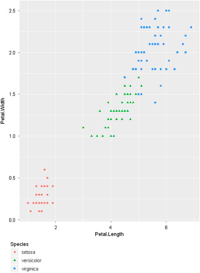
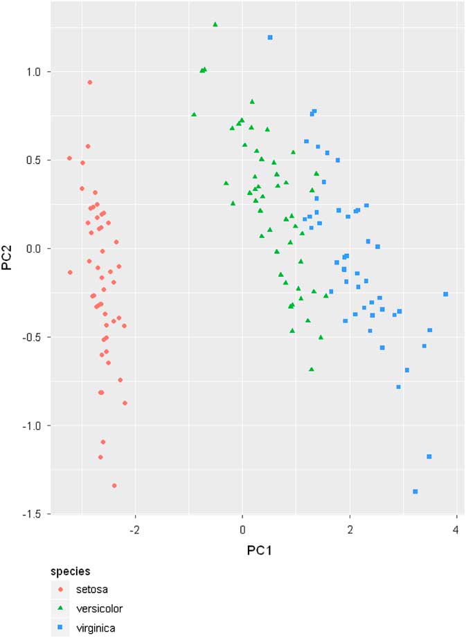
B Visualization Example
C Discretization Example
D Feature Selection Filtering Example
E Outlier and noise detection example
F Principal Component Analysis Example
G Normalization example
H Regression Dataset Example
I Imputation Example
J Imbalanced Dataset and Instance Selection Example