


1. Introduction
Guided by uniqueness of quantum gravity in two dimensions, Witten conjectured in [Reference Witten33] that the generating function of intersection numbers of tautological characteristic classes on the moduli space of stable complex curves has to satisfy the PDE of the Korteweg–de Vries hierarchy. The conjecture was proved a few months later by Kontsevich in his seminal paper [Reference Kontsevich20]. Kontsevich understood that critical graphs of the canonical Strebel differential [Reference Strebel31] on a punctured curve give a cell-decomposition of the moduli space of punctured curves, which can be organised into a novel type of matrix model (the ‘matrix Airy function’) with covariance
 \begin{equation*}\langle \Phi(e_{jk})\Phi(e_{lm})\rangle_c=\frac{\delta_{kl}\delta_{jm}}{ \lambda_j+\lambda_k}\end{equation*}
(where  $(e_{jk})$ denotes the standard matrix basis and
  $\delta_{kl}$ the Kronecker symbol) and tri-valent vertices. The
  $\lambda_j$ are Laplace transform parametersFootnote 1 of the lengths
 $L_j$
of critical trajectories of the Strebel differentials, and the generically simple zeros of the Strebel differential correspond to tri-valent vertices. Kontsevich went on to establish that the logarithm of the partition function of his matrix model is the
$L_j$
of critical trajectories of the Strebel differentials, and the generically simple zeros of the Strebel differential correspond to tri-valent vertices. Kontsevich went on to establish that the logarithm of the partition function of his matrix model is the
 $\tau$
-function for the KdV-hierarchy, thereby proving that his matrix model is integrable.
$\tau$
-function for the KdV-hierarchy, thereby proving that his matrix model is integrable.
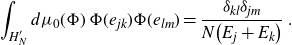
The same covariance (up to normalisation)
 \begin{equation*}\langle \Phi(e_{jk})\Phi(e_{lm})\rangle_c=\frac{\delta_{kl}\delta_{jm}}{ N\!\left(E_j+E_k\right)}\end{equation*}
arises in quantum field theory models on noncommutative geometries [Reference Grosse and Steinacker13], where the
 $E_k$
are the spectral values (‘energy levels’) of a Laplace-type operator. These are models for scalar fields with cubic self-interaction. From a quantum field theoretical point of view one would be more interested in a quartic self-interaction, which e.g. is characteristic to the Higgs field. Such quartic models have been understood in [Reference Grosse and Wulkenhaar15] at the level of formal power series. Later in [Reference Grosse and Wulkenhaar16, Reference Grosse and Wulkenhaar17] exact equations between correlation functions in the quartic (matrix) model were derived. These equations share many aspects with a universal structure called topological recursion [Reference Eynard and Orantin10].
$E_k$
are the spectral values (‘energy levels’) of a Laplace-type operator. These are models for scalar fields with cubic self-interaction. From a quantum field theoretical point of view one would be more interested in a quartic self-interaction, which e.g. is characteristic to the Higgs field. Such quartic models have been understood in [Reference Grosse and Wulkenhaar15] at the level of formal power series. Later in [Reference Grosse and Wulkenhaar16, Reference Grosse and Wulkenhaar17] exact equations between correlation functions in the quartic (matrix) model were derived. These equations share many aspects with a universal structure called topological recursion [Reference Eynard and Orantin10].
Such recursions typically rely on the initial solution of a non-linear problem (for the Kontsevich model achieved in [Reference Makeenko and Semenoff25]). For the quartic model, the corresponding equation (for the planar two-point function of cycle type (0, 1)) is given in (3.2) below. Its solution succeeded in [Reference Grosse, Hock and Wulkenhaar12], via a larger detour. It was assumed that (3.2) converges for
 $N\to \infty$
to an integral equation with Hölder-continuous measure. The special case of constant measure was solved in [Reference Panzer and Wulkenhaar26] with help from computer algebra. Its structure suggested a conjecture for the general case which was proved in [Reference Grosse, Hock and Wulkenhaar12] by residue theorem and Lagrange-Bürmann resummation.
$N\to \infty$
to an integral equation with Hölder-continuous measure. The special case of constant measure was solved in [Reference Panzer and Wulkenhaar26] with help from computer algebra. Its structure suggested a conjecture for the general case which was proved in [Reference Grosse, Hock and Wulkenhaar12] by residue theorem and Lagrange-Bürmann resummation.
This paper provides a novel algebraic geometrical solution strategy for the non-linear equation (3.2) and the affine equation (6.2) (which determines the planar two-point function of cycle type (2, 0)). We (re)prove that these cumulants are compositions of rational functions with a preferred inverse of another rational function
 \begin{equation*} R(z)=z-\frac{\lambda}{N} \sum_{k=1}^d \frac{\varrho_k}{z+\varepsilon_k}\:.\end{equation*}
Building on these results it was understood in [Reference Branahl, Hock and Wulkenhaar3] that derivatives of the partially summed two-point function with respect to the spectral values
 $E_k$
extend to meromorphic differentials
$E_k$
extend to meromorphic differentials
 $\omega_{g,n}$
labelled by genus g and number n of marked points of a complex curve. The
$\omega_{g,n}$
labelled by genus g and number n of marked points of a complex curve. The
 $\omega_{g,n}$
are supplemented by two families of auxiliary functions and satisfy a coupled system of equations. The solution of this system for small
$\omega_{g,n}$
are supplemented by two families of auxiliary functions and satisfy a coupled system of equations. The solution of this system for small
 $-\chi=2g+n-2$
in [Reference Branahl, Hock and Wulkenhaar3] gave strong support for the conjecture that the
$-\chi=2g+n-2$
in [Reference Branahl, Hock and Wulkenhaar3] gave strong support for the conjecture that the
 $\omega_{g,n}$
obey blobbed topological recursion [Reference Borot and Shadrin7] for the spectral curve
$\omega_{g,n}$
obey blobbed topological recursion [Reference Borot and Shadrin7] for the spectral curve
 $\big(x\,:\,\hat{\mathbb{C}}\to\hat{\mathbb{C}}, \omega_{0,1}=xdy,\omega_{0,2}\big)$
given by
$\big(x\,:\,\hat{\mathbb{C}}\to\hat{\mathbb{C}}, \omega_{0,1}=xdy,\omega_{0,2}\big)$
given by
 \begin{equation*} x(z)=R(z)\;,\qquad y(z)=-R({-}z)\;,\qquad \omega_{0,2}(w,z)=\frac{dw\,dz}{(w-z)^2}+\frac{dw\,dz}{(w+z)^2}\;.\end{equation*}
The proof of this conjecture for
 $g=0$
was achieved in [Reference Hock and Wulkenhaar18]. As shown in [Reference Borot and Shadrin7], blobbed topological recursion generates intersection numbers on the moduli space
$g=0$
was achieved in [Reference Hock and Wulkenhaar18]. As shown in [Reference Borot and Shadrin7], blobbed topological recursion generates intersection numbers on the moduli space
 $\overline{\mathcal{M}}_{g,n}$
of stable complex curves. In view of the deep rôle played by the global involution
$\overline{\mathcal{M}}_{g,n}$
of stable complex curves. In view of the deep rôle played by the global involution
 $z\mapsto -z$
[Reference Hock and Wulkenhaar18] we expect that this very natural involution will find a counterpart in the intersection theory encoded in the quartic analogue of the Kontsevich model. Working out the details is a fascinating programme left for the future.
$z\mapsto -z$
[Reference Hock and Wulkenhaar18] we expect that this very natural involution will find a counterpart in the intersection theory encoded in the quartic analogue of the Kontsevich model. Working out the details is a fascinating programme left for the future.
2. Matrix integrals
Let
 $H_{N}$
be the real vector space of self-adjoint
$H_{N}$
be the real vector space of self-adjoint
 $N\times N$
-matrices and
$N\times N$
-matrices and
 $(E_1,\dots, E_{N})$
be not necessarily distinct positive real numbers. By the Bochner–Minlos theorem [Reference Bochner6], combined with the Schur product theorem [Reference Schur27, section 4], there is a unique probability measure
$(E_1,\dots, E_{N})$
be not necessarily distinct positive real numbers. By the Bochner–Minlos theorem [Reference Bochner6], combined with the Schur product theorem [Reference Schur27, section 4], there is a unique probability measure
 $d\mu_0(\Phi)$
on the dual space
$d\mu_0(\Phi)$
on the dual space
 $H^{\prime}_{N}$
with
$H^{\prime}_{N}$
with
 \begin{align}\exp\!\Bigg({-} \frac{1}{2N} \sum_{k,l=1}^{N}\frac{M_{kl}M_{lk}}{E_k+E_l}\Bigg)= \int_{H^{\prime}_{N}} d\mu_0(\Phi) \,e^{\textrm{i} \Phi(M)}\end{align}
for any
 $M=M^*=\sum_{k,l=1}^{N} M_{kl} e_{kl}\in H_{N}$
, where
$M=M^*=\sum_{k,l=1}^{N} M_{kl} e_{kl}\in H_{N}$
, where
 $(e_{kl})$
is the standard matrix basis. The linear forms extend via
$(e_{kl})$
is the standard matrix basis. The linear forms extend via
 $\Phi(M_1+\textrm{i}M_2)\,:\!=\,\Phi(M_1)+\textrm{i}\Phi(M_2)$
to arbitrary complex
$\Phi(M_1+\textrm{i}M_2)\,:\!=\,\Phi(M_1)+\textrm{i}\Phi(M_2)$
to arbitrary complex
 $N\times N$
-matrices. This allows us to evaluate
$N\times N$
-matrices. This allows us to evaluate
 $\Phi(e_{jk})$
and to identify the covariance
$\Phi(e_{jk})$
and to identify the covariance
 \begin{equation*}\int_{H^{\prime}_{N}} d\mu_0(\Phi) \,\Phi(e_{jk})\Phi(e_{lm}) = \frac{\delta_{kl} \delta_{jm}}{N \!\left(E_j+E_k\right)}\;.\end{equation*}
We are going to deform the Gaußian measure (2.1) by a quartic potential,
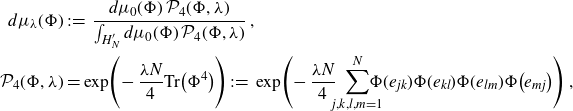 \begin{align}d\mu_\lambda(\Phi) &\,:\!=\,\frac{d\mu_0(\Phi)\; \mathcal{P}_4(\Phi,\lambda)}{\int_{H^{\prime}_{N}} d\mu_0(\Phi)\;\mathcal{P}_4(\Phi,\lambda)}\;,\qquad\\\mathcal{P}_4(\Phi,\lambda)&=\exp\!\Bigg({-}\,\frac{\lambda N}{4} \textrm{Tr}\big(\Phi^4\big)\Bigg)\,:\!=\,\exp\!\Bigg({-}\,\frac{\lambda N}{4} \!\!\sum_{j,k,l,m=1}^{N} \!\!\!\!\! \Phi(e_{jk})\Phi(e_{kl})\Phi(e_{lm})\Phi\big(e_{mj}\big)\Bigg)\;,\nonumber \end{align}
for some
 $\lambda>0$
. This matrix measure is the quartic analogue of the Kontsevich model [Reference Kontsevich20] in which the deformation is given by the cubic term
$\lambda>0$
. This matrix measure is the quartic analogue of the Kontsevich model [Reference Kontsevich20] in which the deformation is given by the cubic term
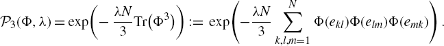 \begin{equation*}\mathcal{P}_3(\Phi,\lambda)=\exp\!\bigg({-}\,\frac{\lambda N}{3} \textrm{Tr}\big(\Phi^3\big)\bigg)\,:\!=\,\exp\!\Bigg({-}\frac{\lambda N}{3}\sum_{k,l,m=1}^{N} \Phi(e_{kl})\Phi(e_{lm})\Phi(e_{mk})\Bigg)\:.\end{equation*}
The cubic measure was designed to prove Witten’s conjecture [Reference Witten33] that intersection numbers of tautological characteristic classes on the moduli space of stable complex curves are related to the KdV hierarchy. Kontsevich proved that
 $\log \int_{H^{\prime}_N} d\mu_0(\Phi)\;\mathcal{P}_3(\Phi, {\textrm{i}}/{2})$
, viewed as function of
$\log \int_{H^{\prime}_N} d\mu_0(\Phi)\;\mathcal{P}_3(\Phi, {\textrm{i}}/{2})$
, viewed as function of
 $t_k=-(2k-1)!!({1}/{N})\sum_{j=1}^{N} E_j^{-(2k+1)}$
, is the generating function of these intersection numbers.
$t_k=-(2k-1)!!({1}/{N})\sum_{j=1}^{N} E_j^{-(2k+1)}$
, is the generating function of these intersection numbers.
We are interested in moments of the measure (2.2),
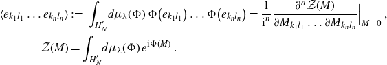 \begin{align}\langle e_{k_1l_1}\dots e_{k_nl_n}\rangle &\,:\!=\, \int_{H^{\prime}_{N}} \!d\mu_\lambda(\Phi)\;\Phi\big(e_{k_1l_1}\big) \ldots \Phi\big(e_{k_nl_n}\big)= \frac{1}{\textrm{i}^{n}}\frac{\partial^n\mathcal{Z}(M)}{\partial M_{k_1l_1}\ldots \partial M_{k_nl_n}} \Big|_{M=0}\;,\nonumber\\\mathcal{Z}(M)&= \int_{H^{\prime}_N}\! d\mu_\lambda(\Phi) \;e^{\textrm{i}\Phi(M)}\;.\end{align}
As explained in Appendix A (see also [Reference McCullagh23, Reference Speed30]), the moments (2.3) decompose into cumulants
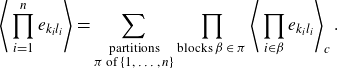 \begin{align}\Bigg\langle \prod_{i=1}^n e_{k_il_i}\Bigg\rangle=\sum_{\substack{\text{partitions} \\ \text{$\pi$ of $\{1,\dots, n\}$}}} \prod_{\text{blocks $\beta \in \pi$}}\Bigg\langle \prod_{i\in \beta} e_{k_i l_i} \Bigg\rangle_c\;.\end{align}
For a quartic potential (2.2), moments and cumulants are only non-zero if n is even and every block
 $\beta$
is of even length. The structure of the Gaußian measure (2.1) (together with the invariance of a trace under cyclic permutations) implies that
$\beta$
is of even length. The structure of the Gaußian measure (2.1) (together with the invariance of a trace under cyclic permutations) implies that
 $\big\langle e_{k_1l_1}\dots e_{k_nl_n}\big\rangle_c$
is only non-zero if
$\big\langle e_{k_1l_1}\dots e_{k_nl_n}\big\rangle_c$
is only non-zero if
 $(l_1,\dots,l_n)=\big(k_{\sigma(1)},\dots,k_{\sigma(n)}\big)$
is a permutation of
$(l_1,\dots,l_n)=\big(k_{\sigma(1)},\dots,k_{\sigma(n)}\big)$
is a permutation of
 $(k_1,\dots,k_n)$
, and in this case the cumulant only depends on the cycle type of this permutation
$(k_1,\dots,k_n)$
, and in this case the cumulant only depends on the cycle type of this permutation
 $\sigma$
in the symmetric group
$\sigma$
in the symmetric group
 $\mathcal{S}_n$
(see Appendix A, with
$\mathcal{S}_n$
(see Appendix A, with
 $b\geqslant 1$
the number of cycles of length
$b\geqslant 1$
the number of cycles of length
 $n_i>0$
,
$n_i>0$
,
 $n_1+\ldots +n_b=n$
):
$n_1+\ldots +n_b=n$
):
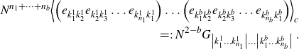 \begin{align}N^{n_1+\dots+n_b}\Big\langle \Big(e_{k_1^1k_2^1}e_{k_2^1k_3^1} \ldots e_{k_{n_1}^1k_1^1}\Big) \ldots\Big(e_{k_1^bk_2^b} e_{k_2^bk_3^b} \ldots e_{k_{n_b}^bk_1^b}\Big) \Big\rangle_c\nonumber\\\,=\!:\,N^{2-b} G_{\big|k_1^1\dots k_{n_1}^1\big|\dots\big|k_1^b\dots k_{n_b}^b\big|} \;.\end{align}
To correctly identify the cycles of the permutation it is necessary that all
 $k^i_j$
are pairwise different in (2.5). These N-rescaled cumulants (2.5) are further expanded as formal power series
$k^i_j$
are pairwise different in (2.5). These N-rescaled cumulants (2.5) are further expanded as formal power series
 $G_{\dots}=\sum_{g=0}^\infty N^{-2g} G_{\dots}^{(g)} $
in
$G_{\dots}=\sum_{g=0}^\infty N^{-2g} G_{\dots}^{(g)} $
in
 $N^{-2}$
so that
$N^{-2}$
so that
 \begin{align}N^{n_1+\dots+n_b} \Big\langle \Big(e_{k_1^1k_2^1}e_{k_2^1k_3^1} \ldots e_{k_{n_1}^1k_1^1}\Big) \ldots\Big(e_{k_1^bk_2^b} e_{k_2^bk_3^b} \ldots e_{k_{n_b}^bk_1^b}\Big) \Big\rangle_c \nonumber\\= \sum_{g=0}^\infty N^{2-b-2g} \cdot G^{(g)}_{\big|k_1^1\dots k_{n_1}^1\big|\dots\big|k_1^b\dots k_{n_b}^b\big|} \;.\end{align}
It turns out that this grading (g, b) of
 $G^{(g)}_{\big|k_1^1\dots k_{n_1}^1\big|\dots \big|k_1^b\dots k_{n_b}^b\big|}$
fits with the combinatorics of ribbon graphs (with 4-valent vertices) on a connected oriented compact topological surface of genus
$G^{(g)}_{\big|k_1^1\dots k_{n_1}^1\big|\dots \big|k_1^b\dots k_{n_b}^b\big|}$
fits with the combinatorics of ribbon graphs (with 4-valent vertices) on a connected oriented compact topological surface of genus
 $g\geqslant 0$
with
$g\geqslant 0$
with
 $b\geqslant 1$
boundary components (and
$b\geqslant 1$
boundary components (and
 $n_i$
labels on the
$n_i$
labels on the
 $i{\text{th}}$
boundary component) and Euler characteristic
$i{\text{th}}$
boundary component) and Euler characteristic
 $\chi=2-2g-b$
(see e.g. [Reference Grosse and Wulkenhaar14, section 3] for the particular case of 4-valent vertices, and compare also with [Reference Kontsevich20] or [Reference Eynard11, sections 2 and 6]). Note that the moments are related to ribbon graphs on possibly non-connected oriented compact topological surfaces (see e.g. [Reference Lando and Zvonkin22, section 3, proposition 3.8.3]).
$\chi=2-2g-b$
(see e.g. [Reference Grosse and Wulkenhaar14, section 3] for the particular case of 4-valent vertices, and compare also with [Reference Kontsevich20] or [Reference Eynard11, sections 2 and 6]). Note that the moments are related to ribbon graphs on possibly non-connected oriented compact topological surfaces (see e.g. [Reference Lando and Zvonkin22, section 3, proposition 3.8.3]).
Starting point for the investigation of cumulants are equations of motion for
 $\mathcal{Z}(M)$
:
$\mathcal{Z}(M)$
:
Lemma 2.1. The Fourier transform
 $\mathcal{Z}(M)$
of the measure (2.2) satisfies
$\mathcal{Z}(M)$
of the measure (2.2) satisfies
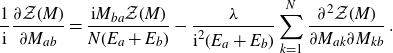
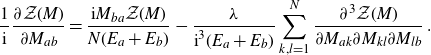 \begin{align}\frac{1}{\textrm{i}}\frac{\partial \mathcal{Z}(M)}{\partial M_{ab}}= \frac{\textrm{i} M_{ba}\mathcal{Z}(M)}{N(E_a+E_b)}-\frac{\lambda }{\textrm{i}^3(E_a+E_b)}\sum_{k,l=1}^{N} \frac{\partial^3\mathcal{Z}(M)}{\partial M_{ak}\partial M_{kl}\partial M_{lb}}\;.\end{align}
Proof. This follows from basic properties of the Gaußian measure (2.1). The derivative
 $({1}/{\textrm{i}})({\partial}/{\partial M_{ab}})$
applied to
$({1}/{\textrm{i}})({\partial}/{\partial M_{ab}})$
applied to
 $\mathcal{Z}(M)$
produces a factor
$\mathcal{Z}(M)$
produces a factor
 $\Phi(e_{ab})$
under the integral. Moments of
$\Phi(e_{ab})$
under the integral. Moments of
 $d\mu_0(\Phi)$
are by (2.2) a sum over pairings. This means that
$d\mu_0(\Phi)$
are by (2.2) a sum over pairings. This means that
 $\Phi(e_{ab})$
is paired in all possible ways with a
$\Phi(e_{ab})$
is paired in all possible ways with a
 $\Phi(e_{cd})$
contained in
$\Phi(e_{cd})$
contained in
 $\exp\!(\textrm{i} \Phi(M))$
or in
$\exp\!(\textrm{i} \Phi(M))$
or in
 $\mathcal{P}_4(\Phi,\lambda)$
. Every such pair contributes a factor
$\mathcal{P}_4(\Phi,\lambda)$
. Every such pair contributes a factor
 $\delta_{ad}\delta_{bc}/\big(N\big(E_a+E_b\big)\big)$
, and summing over all pairings is the same as taking the derivative, thus producing a term
$\delta_{ad}\delta_{bc}/\big(N\big(E_a+E_b\big)\big)$
, and summing over all pairings is the same as taking the derivative, thus producing a term
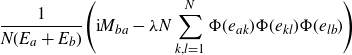 \begin{equation*}\frac{1}{N(E_a+E_b)}\Bigg(\textrm{i} M_{ba}-\lambda N\sum_{k,l=1}^{N} \Phi(e_{ak})\Phi(e_{kl})\Phi(e_{lb})\Bigg)\end{equation*}
under the integral. The triple product of
 $\Phi(e_{..})$
is written as a third derivative with respect to the corresponding entries of M.
$\Phi(e_{..})$
is written as a third derivative with respect to the corresponding entries of M.
The Kontsevich model [Reference Kontsevich20] with cubic deformation
 $\mathcal{P}_3(\Phi,\lambda)$
is governed by the equation of motion
$\mathcal{P}_3(\Phi,\lambda)$
is governed by the equation of motion
 \begin{equation*}\frac{1}{\textrm{i}}\frac{\partial \mathcal{Z}(M)}{\partial M_{ab}} = \frac{\textrm{i} M_{ba}\mathcal{Z}(M)}{N(E_a+E_b)} -\frac{\lambda }{\textrm{i}^2 (E_a+E_b)} \sum_{k=1}^{N} \frac{\partial^2 \mathcal{Z}(M)}{\partial M_{ak} \partial M_{kb}} \:.\end{equation*}
For
 $N=1$
this is essentially the ODE
$N=1$
this is essentially the ODE
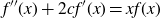 \begin{equation*}f^{\prime\prime}(x)+2c f^{\prime}(x)=x f(x)\end{equation*}
solved by the Airy function
 $f(x)=e^{-cx} \textrm{Ai}(x+c^2)$
, hence the title of [Reference Kontsevich20]. Its quartic analogue is the matrix version of the ODE
$f(x)=e^{-cx} \textrm{Ai}(x+c^2)$
, hence the title of [Reference Kontsevich20]. Its quartic analogue is the matrix version of the ODE
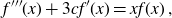 \begin{equation*}f^{\prime\prime\prime}(x)+3c f^{\prime}(x)=x f(x)\:,\end{equation*}
which does not seem to have a name. The Airy function is the case
 $p=2$
of a larger class
$p=2$
of a larger class
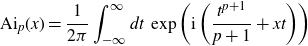 \begin{equation*}\textrm{Ai}_p(x)=\frac{1}{2\pi} \int_{-\infty}^\infty dt \; \exp\left( \mathrm{i} \left(\frac{t^{p+1}}{p+1}+xt\right)\right)\end{equation*}
of higher Airy functions. As remarked in [Reference Kontsevich20, section 4.3], they also give rise to higher matrix Airy functions. In particular, there is also a ‘quartic analogue’
 $p=3$
in this class, which was studied in [Reference Itzykson and Zuber19, Reference Kristjansen21]. This matrix model does not seem to be related to our ‘quartic analogue’ of the Kontsevich model.
$p=3$
in this class, which was studied in [Reference Itzykson and Zuber19, Reference Kristjansen21]. This matrix model does not seem to be related to our ‘quartic analogue’ of the Kontsevich model.
Another equation of motion will be necessary for the subsequent work in [Reference Branahl, Hock and Wulkenhaar3]:
Lemma 2.2. The Fourier transform
 $\mathcal{Z}(M)$
of the measure (2.2) satisfies
$\mathcal{Z}(M)$
of the measure (2.2) satisfies
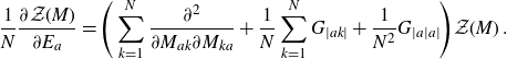 \begin{align}\frac{1}{N} \frac{\partial \mathcal{Z}(M)}{\partial E_{a}}= \Bigg(\sum_{k=1}^N\frac{\partial^2}{\partial M_{ak} \partial M_{ka}}+ \frac{1}{N}\sum_{k=1}^N G_{|ak|}+\frac{1}{N^2}G_{|a|a|}\Bigg)\mathcal{Z}(M)\;.\end{align}
Proof. Application of
 $(1/N)(\partial/\partial E_a)-\!\sum_{k=1}^N \partial^2/\big(\partial M_{ak} \partial M_{ka}\big)-(1/N)\sum_{k=1}^N\! 1/\big(E_a+E_k\big)$
to the left-hand side of (2.1) yields zero so that it gives
$(1/N)(\partial/\partial E_a)-\!\sum_{k=1}^N \partial^2/\big(\partial M_{ak} \partial M_{ka}\big)-(1/N)\sum_{k=1}^N\! 1/\big(E_a+E_k\big)$
to the left-hand side of (2.1) yields zero so that it gives
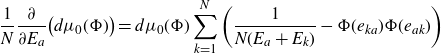 \begin{align*}\frac{1}{N}\frac{\partial}{\partial E_a}\big(d\mu_0(\Phi)\big)= d\mu_0(\Phi)\sum_{k=1}^N \bigg(\frac{1}{N(E_a+E_k)}-\Phi(e_{ka})\Phi(e_{ak})\bigg)\end{align*}
when applying it to the right-hand side. Apply this identity to (2.2) to get
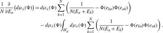 \begin{align*}\frac{1}{N} \frac{\partial}{\partial E_a}\big(d\mu_\lambda(\Phi)\big) &= d\mu_\lambda(\Phi)\sum_{k=1}^N \bigg(\frac{1}{N(E_a+E_k)}-\Phi(e_{ka})\Phi(e_{ak})\bigg)\nonumber\\& \quad- d\mu_\lambda(\Phi) \!\! \int_{H^{\prime}_{N}} d\mu_\lambda(\Phi) \sum_{k=1}^N \bigg(\frac{1}{N(E_a+E_k)}-\Phi(e_{ka})\Phi(e_{ak})\bigg)\;.\end{align*}
Multiplying with
 $e^{\textrm{i}\Phi(M)}$
and integrating over
$e^{\textrm{i}\Phi(M)}$
and integrating over
 $H^{\prime}_N$
gives with (A3) the assertion.
$H^{\prime}_N$
gives with (A3) the assertion.
The equations of motion (2.7) and (2.8) induce identities between cumulants. Some of them are derived in Appendix B, for others see [Reference Grosse and Wulkenhaar17]. Taking also the grading by (g, b) into account, one can establish a partial order in the homogeneous building blocks
 $G^{(g)}_{\dots}$
. The least element is the planar two-point function
$G^{(g)}_{\dots}$
. The least element is the planar two-point function
 $G_{|ab|}^{(0)}$
, which is the dominant part (at large N) of the cumulant of length 2 and cycle type (0, 1) (i.e. one cycle ab of length 2). It satisfies a closed non-linear equation for it alone, given in (3.1) below. Any other homogeneous building block of (2.6) satisfies an affine equation with inhomogeneity that depends only on functions of strictly larger topological Euler characteristic
$G_{|ab|}^{(0)}$
, which is the dominant part (at large N) of the cumulant of length 2 and cycle type (0, 1) (i.e. one cycle ab of length 2). It satisfies a closed non-linear equation for it alone, given in (3.1) below. Any other homogeneous building block of (2.6) satisfies an affine equation with inhomogeneity that depends only on functions of strictly larger topological Euler characteristic
 $\chi=2-2g-b$
, which are known by induction. Similar recursive systems have been identified in many areas of mathematics. Their common universal structure has been axiomatised under the name topological recursion [Reference Eynard and Orantin10], since the recursion is by the topological Euler characteristic. Starting from a few initial data called the spectral curve, topological recursion constructs a hierarchy of differential forms and understands them as spectral invariants of the curve. A prominent example is the Kontsevich model [Reference Kontsevich20] whose topological recursion is described e.g. in [Reference Eynard11, section 6]. Other classes of examples are the one- and two-matrix models [Reference Chekhov, Eynard and Orantin8], Mirzakhani’s recursions [Reference Mirzakhani24] for the volume of moduli spaces of Riemann surfaces, and recursions in Hurwitz theory [Reference Bouchard and Mariño5] and Gromov–Witten theory [Reference Bouchard, Klemm, Mariño and Pasquetti4].
$\chi=2-2g-b$
, which are known by induction. Similar recursive systems have been identified in many areas of mathematics. Their common universal structure has been axiomatised under the name topological recursion [Reference Eynard and Orantin10], since the recursion is by the topological Euler characteristic. Starting from a few initial data called the spectral curve, topological recursion constructs a hierarchy of differential forms and understands them as spectral invariants of the curve. A prominent example is the Kontsevich model [Reference Kontsevich20] whose topological recursion is described e.g. in [Reference Eynard11, section 6]. Other classes of examples are the one- and two-matrix models [Reference Chekhov, Eynard and Orantin8], Mirzakhani’s recursions [Reference Mirzakhani24] for the volume of moduli spaces of Riemann surfaces, and recursions in Hurwitz theory [Reference Bouchard and Mariño5] and Gromov–Witten theory [Reference Bouchard, Klemm, Mariño and Pasquetti4].
3. The planar two-point function
The two-point function
 $G_{|ab|}$
is the cumulant of length 2 and cycle type (0, 1) (i.e. one cycle ab of length 2), see Appendix A. We reprove in Appendix B that the planar two-point function
$G_{|ab|}$
is the cumulant of length 2 and cycle type (0, 1) (i.e. one cycle ab of length 2), see Appendix A. We reprove in Appendix B that the planar two-point function
 $G^{(0)}_{|ab|}$
(of degree or genus
$G^{(0)}_{|ab|}$
(of degree or genus
 $g=0$
) satisfies
$g=0$
) satisfies
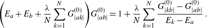 \begin{align}\Bigg(E_a+E_b+\frac{\lambda}{N}\sum_{k=1}^{N} G^{(0)}_{|ak|}\Bigg)G^{(0)}_{|ab|}= 1+ \frac{\lambda}{N} \sum_{k=1}^{N}\frac{G^{(0)}_{|kb|}-G^{(0)}_{|ab|}}{E_k-E_a}\;.\end{align}
This equation was first established in [Reference Grosse and Wulkenhaar16]; equation (B7) which involves all
 $G^{(g)}_{|ab|}$
was obtained in [Reference Grosse and Wulkenhaar17].
$G^{(g)}_{|ab|}$
was obtained in [Reference Grosse and Wulkenhaar17].
To give a meaning to the term
 $k=a$
in (3.1) we make the decisive assumption that
$k=a$
in (3.1) we make the decisive assumption that
 $\Big\{G^{(0)}_{|ab|}\Big\}_{a,b=1,\dots N}$
arise by evaluation of a holomorphic function in two complex variables. Let
$\Big\{G^{(0)}_{|ab|}\Big\}_{a,b=1,\dots N}$
arise by evaluation of a holomorphic function in two complex variables. Let
 $E_1,\dots,E_d$
be the distinct entries in the tuple
$E_1,\dots,E_d$
be the distinct entries in the tuple
 $(E_k)$
, which occur with multiplicities
$(E_k)$
, which occur with multiplicities
 $r_1,\dots,r_d$
, with
$r_1,\dots,r_d$
, with
 $N=r_1+\dots+r_d$
. We assume that for some neighbourhoods
$N=r_1+\dots+r_d$
. We assume that for some neighbourhoods
 $\mathcal{U}_k\subset \mathbb{C}$
of
$\mathcal{U}_k\subset \mathbb{C}$
of
 $E_k$
there is a holomorphic function
$E_k$
there is a holomorphic function
 $G^{(0)}\,:\, \bigcup_{k,l=1}^d \!(\mathcal{U}_k\times \mathcal{U}_l)\to \mathbb{C}$
which interpolates
$G^{(0)}\,:\, \bigcup_{k,l=1}^d \!(\mathcal{U}_k\times \mathcal{U}_l)\to \mathbb{C}$
which interpolates
 $G^{(0)}_{|ab|}=G^{(0)}(E_a,E_b)$
and satisfies the natural (but by no means unique) holomorphic extension
$G^{(0)}_{|ab|}=G^{(0)}(E_a,E_b)$
and satisfies the natural (but by no means unique) holomorphic extension
 \begin{align}\Bigg(\zeta+\eta+\frac {\lambda}{N}\sum_{k=1}^d r_k G^{(0)}(\zeta,E_k)\Bigg)G^{(0)}(\zeta,\eta)&=1+\frac{\lambda}{N} \sum_{k=1}^d r_k\frac{G^{(0)}(E_k,\eta)-G^{(0)}(\zeta,\eta)}{E_k-\zeta}\end{align}
of (3.1), for
 $(\zeta,\eta)\in \bigcup_{k,l=1}^d \!(\mathcal{U}_k\times \mathcal{U}_l)$
. Equation (3.1) is understood as the limit
$(\zeta,\eta)\in \bigcup_{k,l=1}^d \!(\mathcal{U}_k\times \mathcal{U}_l)$
. Equation (3.1) is understood as the limit
 $\zeta\to E_a$
and
$\zeta\to E_a$
and
 $\eta\to E_b$
of (3.2) when taking multiplicities into account. It is not possible to deduce (3.2) from (3.1) alone. Justification of (3.2) comes from the fact that it gives rise to interesting mathematical structures:
$\eta\to E_b$
of (3.2) when taking multiplicities into account. It is not possible to deduce (3.2) from (3.1) alone. Justification of (3.2) comes from the fact that it gives rise to interesting mathematical structures:
Theorem 3.1. Construct 2d functions
 $\{\varepsilon_k(\lambda),\varrho_k(\lambda)\}_{k=1,\dots,d}$
, with
$\{\varepsilon_k(\lambda),\varrho_k(\lambda)\}_{k=1,\dots,d}$
, with
 $\lim_{\lambda\to 0} \big(\varepsilon_k,\varrho_k\big)=\big(E_k,r_k\big)$
, as implicitly defined solution of the system
$\lim_{\lambda\to 0} \big(\varepsilon_k,\varrho_k\big)=\big(E_k,r_k\big)$
, as implicitly defined solution of the system
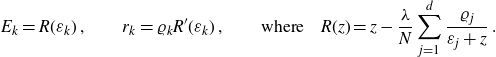 \begin{align}E_k=R(\varepsilon_k)\;,\qquad r_k=\varrho_k R^{\prime}(\varepsilon_k)\;,\qquad \text{where}\quad R(z)=z-\frac{\lambda}{N}\sum_{j=1}^d \frac{\varrho_j}{\varepsilon_j+z}\;.\end{align}
Then (3.2) is solved by
 $G^{(0)}(\zeta,\eta)=\mathcal{G}^{(0)}\big(R^{-1}(\zeta),R^{-1}(\eta)\big)$
, where
$G^{(0)}(\zeta,\eta)=\mathcal{G}^{(0)}\big(R^{-1}(\zeta),R^{-1}(\eta)\big)$
, where
 $\mathcal{G}^{(0)}\,:\,\hat{\mathbb{C}}\times \hat{\mathbb{C}} \to\hat{\mathbb{C}}$
is the rational function
$\mathcal{G}^{(0)}\,:\,\hat{\mathbb{C}}\times \hat{\mathbb{C}} \to\hat{\mathbb{C}}$
is the rational function
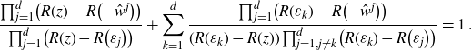
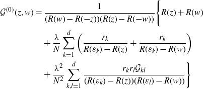 \begin{align}\mathcal{G}^{(0)}(z,w)&=\frac{1}{(R(w)-R({-}z))(R(z)-R({-}w))}\Bigg\{R(z)+R(w)\nonumber\\& \quad +\frac{\lambda}{N}\sum_{k=1}^d \bigg(\frac{r_k}{R(\varepsilon_k)-R(z)}+\frac{r_k}{R(\varepsilon_k)-R(w)}\bigg)\nonumber\\& \quad +\frac{\lambda^2}{N^2}\sum_{k,l=1}^d \frac{r_k r_l \mathcal{G}_{kl}}{(R(\varepsilon_k)-R(z))(R(\varepsilon_l)-R(w))}\Bigg\}\end{align}
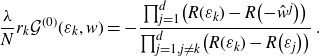
with
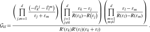 \begin{align}\mathcal{G}_{kl}=\frac{\displaystyle\Bigg(\prod_{j,m=1}^d \frac{\big({-}\widehat{\varepsilon_k}^j-\widehat{\varepsilon_l}^m\big)}{\varepsilon_j+\varepsilon_m}\Bigg)\left(\prod_{\substack{j=1\\j\neq k}}^d \frac{\varepsilon_k-\varepsilon_j}{R(\varepsilon_k){-}R\big(\varepsilon_j\big)}\right)\left(\prod_{\substack{m=1\\m\neq l}}^d \frac{\varepsilon_l-\varepsilon_m}{R(\varepsilon_l){-}R(\varepsilon_m)}\right)}{R^{\prime}(\varepsilon_k)R^{\prime}(\varepsilon_l) (\varepsilon_k+\varepsilon_l)} \;.\end{align}
Here
 $z\in \big\{u,\hat{u}^1,\dots,\hat{u}^d\big\}$
is the list of the different roots of
$z\in \big\{u,\hat{u}^1,\dots,\hat{u}^d\big\}$
is the list of the different roots of
 $R(z)=R(u)$
, and the correct branch of
$R(z)=R(u)$
, and the correct branch of
 $R^{-1}$
is chosen by the implicitly defined solutions above (i.e.
$R^{-1}$
is chosen by the implicitly defined solutions above (i.e.
 $\varepsilon_k \in R^{-1}(\mathcal{U}_k)$
for this branch). In particular,
$\varepsilon_k \in R^{-1}(\mathcal{U}_k)$
for this branch). In particular,
 $G^{(0)}_{|kl|}=\mathcal{G}^{(0)}(\varepsilon_k,\varepsilon_l)\equiv\mathcal{G}_{kl}$
solves (3.1).
$G^{(0)}_{|kl|}=\mathcal{G}^{(0)}(\varepsilon_k,\varepsilon_l)\equiv\mathcal{G}_{kl}$
solves (3.1).
Existence of
 $(\varepsilon_k(\lambda),\varrho_k(\lambda))$
in a neighbourhood of
$(\varepsilon_k(\lambda),\varrho_k(\lambda))$
in a neighbourhood of
 $\lambda=0$
is guaranteed by the implicit function theorem. We will prove several equivalent formulae for
$\lambda=0$
is guaranteed by the implicit function theorem. We will prove several equivalent formulae for
 $\mathcal{G}^{(0)}(z,w)$
: (4.5), (4.9), (4.14) and eventually (3.4). Some of them were already proved in [Reference Grosse, Hock and Wulkenhaar12]. There, inspired by the solution of a particular case [Reference Panzer and Wulkenhaar26], equation (3.2) was interpreted as an integral equation for a Dirac measure. Approximating the Dirac measure by a Hölder-continuous function allowed to employ boundary values techniques for sectionally holomorphic functions. Residue theorem and Lagrange–Bürmann resummation gave a solution formula whose limit back to Dirac measure was arranged into (4.14).
$\mathcal{G}^{(0)}(z,w)$
: (4.5), (4.9), (4.14) and eventually (3.4). Some of them were already proved in [Reference Grosse, Hock and Wulkenhaar12]. There, inspired by the solution of a particular case [Reference Panzer and Wulkenhaar26], equation (3.2) was interpreted as an integral equation for a Dirac measure. Approximating the Dirac measure by a Hölder-continuous function allowed to employ boundary values techniques for sectionally holomorphic functions. Residue theorem and Lagrange–Bürmann resummation gave a solution formula whose limit back to Dirac measure was arranged into (4.14).
In this paper we provide a more elementary proof of these equations which solely needs properties of Cauchy matrices established by Schechter [Reference Schechter28]:
Proposition 3.2 ([Reference Schechter28]). For two d-tuples
 $(a_1,\dots,a_d)$
and
$(a_1,\dots,a_d)$
and
 $(b_1,\dots,b_d)$
, with all
$(b_1,\dots,b_d)$
, with all
 $a_i,b_j$
distinct, consider the
$a_i,b_j$
distinct, consider the
 $d\times d$
-matrix
$d\times d$
-matrix
 $H=\big(\frac{1}{a_k-b_l}\big)_{kl}$
. Let
$H=\big(\frac{1}{a_k-b_l}\big)_{kl}$
. Let
 $A(x)\,:\!=\,\prod_{i=1}^d\! (x-a_i)$
and
$A(x)\,:\!=\,\prod_{i=1}^d\! (x-a_i)$
and
 $B(y)\,:\!=\,\prod_{j=1}^d\! (y-b_j)$
. Then the inverse of H is given by
$B(y)\,:\!=\,\prod_{j=1}^d\! (y-b_j)$
. Then the inverse of H is given by
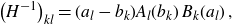 \begin{align}\big(H^{-1}\big)_{kl}= (a_l-b_k) A_l(b_k)\,B_k(a_l)\;,\end{align}
where
 $A_l,B_k$
are the Lagrange interpolation polynomials
$A_l,B_k$
are the Lagrange interpolation polynomials
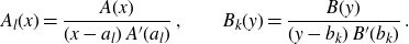 \begin{align}A_l(x)=\frac{A(x)}{(x-a_l) \,A^{\prime}(a_l)}\;,\qquad B_k(y)=\frac{B(y)}{(y-b_k) \,B^{\prime}(b_k)}\;.\end{align}
The inverse of H satisfies
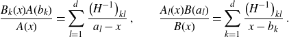 \begin{align}\frac{B_k(x)A(b_k)}{A(x)}=\sum_{l=1}^d \frac{\big(H^{-1}\big)_{kl}}{a_l-x}\;,\qquad \frac{A_l(x)B(a_l)}{B(x)}=\sum_{k=1}^d \frac{\big(H^{-1}\big)_{kl}}{x-b_k}\;.\end{align}
Moreover, the row sums and column sums of
 $H^{-1}$
are given by
$H^{-1}$
are given by
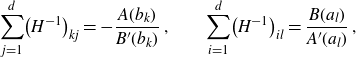 \begin{align}\sum_{j=1}^d \!\big(H^{-1}\big)_{kj}=-\frac{A(b_k)}{B^{\prime}(b_k)}\;,\qquad \sum_{i=1}^d \!\big(H^{-1}\big)_{il}=\frac{B(a_l)}{A^{\prime}(a_l)}\;,\end{align}
and one has, for all
 $j=1,\dots, d$
,
$j=1,\dots, d$
,
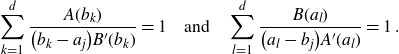 \begin{align}\sum_{k=1}^d \frac{A(b_k)}{\big(b_k-a_j\big) B^{\prime}(b_k)}=1\quad \text{and}\quad \sum_{l=1}^d \frac{B(a_l)}{\big(a_l-b_j\big) A^{\prime}(a_l)}=1\;.\end{align}
4. Proof of Theorem 3.1
We are going to construct a non-constant rational function
 $R\in\mathbb{C}(z)$
viewed as a branched cover
$R\in\mathbb{C}(z)$
viewed as a branched cover
 $R\,:\,\hat{\mathbb{C}}=\mathbb{C}\cup\{\infty\}\to\hat{\mathbb{C}}=\mathbb{C}\cup\{\infty\}$
of Riemann surfaces (with
$R\,:\,\hat{\mathbb{C}}=\mathbb{C}\cup\{\infty\}\to\hat{\mathbb{C}}=\mathbb{C}\cup\{\infty\}$
of Riemann surfaces (with
 $z=\textrm{id}_{\mathbb{C}}$
the standard coordinate on
$z=\textrm{id}_{\mathbb{C}}$
the standard coordinate on
 $\mathbb{C}$
) via the following:
$\mathbb{C}$
) via the following:
Ansatz 4.1. A branched cover
 $R\,:\,\hat{\mathbb{C}}\to\hat{\mathbb{C}}$
is supposed to be determined by conventions (i)–(vi) and an algebraic relation (vii):
$R\,:\,\hat{\mathbb{C}}\to\hat{\mathbb{C}}$
is supposed to be determined by conventions (i)–(vi) and an algebraic relation (vii):
-
(i) R has degree
 $d+1$
;
$d+1$
; -
(ii) all ramification points of R do not belong to
$R^{-1}(\{E_1,\dots,E_d\})$
; -
(iii) without loss of generality,
$R(\infty)=\infty$
with residue
$-1$
in the sense that
$ \textrm{Res}_{z= \infty} R(z)dz=-1$
; -
(iv) for every
$k=1,\dots, d$
, distinguish any of the
$d{+}1$
distinct points of the fibre
$R^{-1}(E_k)$
as
$\varepsilon_k$
. Take any connected neighbourhood
$\mathcal{U}_k\subset \mathbb{C}$
of
$E_k$
for which
$R^{-1}(\mathcal{U}_k)$
has
$d{+}1$
connected components, and let
$\mathcal{V}_k$
be the connected component of
$R^{-1}(\mathcal{U}_k)$
which contains
$\varepsilon_k$
. Then the choice of
$\{\varepsilon_k\}$
determines a holomorphic function
$\mathcal{G}^{(0)}\,:\,\bigcup_{k,l=1}^d \!(\mathcal{V}_k\times \mathcal{V}_l) \to \mathbb{C}$
by
$\mathcal{G}^{(0)}(z,w)=G^{(0)}(R(z),R(w))$
, where
$G^{(0)}\,:\,\bigcup_{k,l=1}^d \!(\mathcal{U}_k\times \mathcal{U}_l)\to \mathbb{C}$
satisfies (3.2); -
(v) for any
$w\in \bigcup_{j=1}^d\mathcal{V}_j$
, let
$\hat{w}^1,\dots,\hat{w}^d$
be the d other distinct preimages of
$R(w)\in \bigcup_{j=1}^d\mathcal{U}_j$
under R, i.e.
$R\big(\hat{w}^k\big)=R(w)$
. Assume that for all
\begin{equation*}\infty\neq R\big({-}\hat{w}^l\big) \quad \text{and} \quad R\big({-}\hat{w}^l\big) \neq R\big({-}\hat{w}^{l^{\prime}}\big)\end{equation*}
$l, l^{\prime}=1,\dots,d$
with
$l\neq l^{\prime}$
and w close to some
$\varepsilon_k$
;
-
(vi) for any w close to some
$\varepsilon_k$
,
$\mathcal{G}^{(0)}\big({-}\hat{w}^l,w\big)$
is defined and finite for all
$l=1,\dots,d$
. This is the case e.g. if
$-\hat{w}^l\in \bigcup_{j=1}^d\mathcal{V}_j$
for all
$l=1,\dots,d$
, or if
$\mathcal{G}^{(0)}$
extends to a suitable rational function on
$\hat{\mathbb{C}}\times \hat{\mathbb{C}}$
; -
(vii) for any
$z\in \mathcal{V}_l$
one has (4.1)
\begin{align} R(z)+\frac{\lambda}{N}\sum_{k=1}^dr_k \mathcal{G}^{(0)}(z,\varepsilon_k)+ \frac{\lambda}{N} \sum_{k=1}^d \frac{r_k}{R(\varepsilon_k)-R(z)}=-R({-}z).\end{align}


With the properties (iv) and (vii) in this Ansatz 4.1 we turn (3.2) into
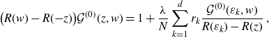 \begin{align}\big(R(w)-R({-}z)\big)\mathcal{G}^{(0)}(z,w) =1+\frac{\lambda}{N} \sum_{k=1}^d r_k\frac{\mathcal{G}^{(0)}(\varepsilon_k,w)}{R(\varepsilon_k)-R(z)}\;,\end{align}
where
 $(z,w)\in \bigcup_{k,l=1}^d \!(\mathcal{V}_k\times\mathcal{V}_l)$
. Next, setting
$(z,w)\in \bigcup_{k,l=1}^d \!(\mathcal{V}_k\times\mathcal{V}_l)$
. Next, setting
 $z=-\hat{w}^l$
in (4.2) for
$z=-\hat{w}^l$
in (4.2) for
 $l=1,\dots,d$
and a given w close to some
$l=1,\dots,d$
and a given w close to some
 $\varepsilon_k$
, requirements (v) and (vi) of Ansatz 4.1 give (by
$\varepsilon_k$
, requirements (v) and (vi) of Ansatz 4.1 give (by
 $\infty\neq R\big({-}\hat{w}^l\big)$
and
$\infty\neq R\big({-}\hat{w}^l\big)$
and
 $\mathcal{G}^{(0)}\big({-}\hat{w}^l,w\big)$
is defined and finite) the d equations
$\mathcal{G}^{(0)}\big({-}\hat{w}^l,w\big)$
is defined and finite) the d equations
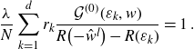 \begin{align}\frac{\lambda}{N}\sum_{k=1}^d r_k \frac{\mathcal{G}^{(0)}(\varepsilon_k,w)}{R\big({-}\hat{w}^l\big)-R(\varepsilon_k)}=1\;.\end{align}
This identifies
 $({\lambda}/{N}) r_k\mathcal{G}^{(0)}(\varepsilon_k,w)$
as row sums of the inverse of a Cauchy matrix. Setting
$({\lambda}/{N}) r_k\mathcal{G}^{(0)}(\varepsilon_k,w)$
as row sums of the inverse of a Cauchy matrix. Setting
 $a_j=R\big({-}\hat{w}^j\big)$
and
$a_j=R\big({-}\hat{w}^j\big)$
and
 $b_i=R(\varepsilon_i)$
in the first identity (3.9) in Proposition 3.2 we conclude (since the
$b_i=R(\varepsilon_i)$
in the first identity (3.9) in Proposition 3.2 we conclude (since the
 $a_j,b_i$
for
$a_j,b_i$
for
 $j,i=1,\dots,d$
are pairwise distinct by requirement (v) of Ansatz 4.1):
$j,i=1,\dots,d$
are pairwise distinct by requirement (v) of Ansatz 4.1):
Corollary 4.2. With Ansatz 4.1 one has
 \begin{align}\frac{\lambda}{N} r_k \mathcal{G}^{(0)}(\varepsilon_k,w)= -\frac{\prod_{j=1}^d \!\big(R(\varepsilon_k)-R\big({-}\hat{w}^j\big)\big)}{\prod_{j=1,j\neq k}^d \!\big(R(\varepsilon_k)-R\big(\varepsilon_j\big)\big)}\;.\end{align}
Inserted back into (4.2) expresses
 $\mathcal{G}^{(0)}(z,w)$
in terms of R. The result simplifies:
$\mathcal{G}^{(0)}(z,w)$
in terms of R. The result simplifies:
Lemma 4.3. With Ansatz 4.1 one has
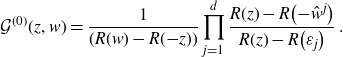 \begin{align}\mathcal{G}^{(0)}(z,w)=\frac{1}{(R(w)-R({-}z))} \prod_{j=1}^d\frac{R(z)-R\big({-}\hat{w}^j\big)}{R(z)-R\big(\varepsilon_j\big)}\;.\end{align}
Proof. This follows from (3.10) for
 $(d+1)$
-tuples with index 0 prepended. Setting
$(d+1)$
-tuples with index 0 prepended. Setting
 $b_0=R(z)$
,
$b_0=R(z)$
,
 $b_k=R(\varepsilon_k)$
,
$b_k=R(\varepsilon_k)$
,
 $a_l=R\big({-}\hat{w}^l\big)$
for
$a_l=R\big({-}\hat{w}^l\big)$
for
 $k,l=1,\dots,d$
, then the case
$k,l=1,\dots,d$
, then the case
 $j=0$
of the first identity (3.10) reads (independent of
$j=0$
of the first identity (3.10) reads (independent of
 $a_0$
)
$a_0$
)
 \begin{align}\frac{\prod_{j=1}^d \!\big(R(z)-R\big({-}\hat{w}^j\big)\big)}{\prod_{j=1}^d \!\big(R(z)-R\big(\varepsilon_j\big)\big)}+ \sum_{k=1}^d \frac{\prod_{j=1}^d \!\big(R(\varepsilon_k)-R\big({-}\hat{w}^j\big)\big)}{(R(\varepsilon_k)-R(z))\prod_{j=1,j\neq k}^d \!\big(R(\varepsilon_k)-R\big(\varepsilon_j\big)\big)}=1\;.\end{align}
Equation (4.5) results from this identity when inserting (4.4) into (4.2).
Lemma 4.4. With Ansatz 4.1 the rational function
 $R\in\mathbb{C}(z)$
is necessarily given by
$R\in\mathbb{C}(z)$
is necessarily given by
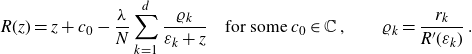 \begin{align}R(z)=z+c_0-\frac{\lambda}{N}\sum_{k=1}^d \frac{\varrho_k}{\varepsilon_k+z}\quad \text{for some } c_0\in \mathbb{C}\;,\qquad \varrho_k=\frac{r_k}{R^{\prime}(\varepsilon_k)}\;.\end{align}
Proof. Comparing the limit
 $z\to \varepsilon_k$
of (4.5) with (4.4) shows that R has a simple pole at every
$z\to \varepsilon_k$
of (4.5) with (4.4) shows that R has a simple pole at every
 $-\varepsilon_k$
with
$-\varepsilon_k$
with
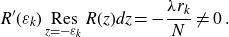 \begin{equation*}{R^\prime }({\varepsilon _k})\mathop {{\rm{RES}}}\limits_{z = - {\varepsilon _k}} \,R(z)dz = - \frac{{\lambda {r_k}}}{N} \ne 0\:.\end{equation*}
By construction, R has also a pole at
 $\infty$
. Since R has degree
$\infty$
. Since R has degree
 $d+1$
by (i) in Ansatz 4.1,
$d+1$
by (i) in Ansatz 4.1,
 $\{-\varepsilon_1,\dots, -\varepsilon_d,\infty\}$
is already the complete list of poles (i.e. preimages of
$\{-\varepsilon_1,\dots, -\varepsilon_d,\infty\}$
is already the complete list of poles (i.e. preimages of
 $\infty$
) of R. Moreover, the pole at
$\infty$
) of R. Moreover, the pole at
 $\infty$
has to be simple with
$\infty$
has to be simple with
 $\lim_{z\to\infty} {R(z)}/{z}=1$
by (iii) in Ansatz 4.1. Therefore,
$\lim_{z\to\infty} {R(z)}/{z}=1$
by (iii) in Ansatz 4.1. Therefore,
 $R(z)-z+ ({\lambda}/{N}) \sum_{k=1}^d {\varrho_k}/({\varepsilon_k+z})$
is a bounded holomorphic function on
$R(z)-z+ ({\lambda}/{N}) \sum_{k=1}^d {\varrho_k}/({\varepsilon_k+z})$
is a bounded holomorphic function on
 $\hat{\mathbb{C}}$
, which by Liouville’s theorem is a constant
$\hat{\mathbb{C}}$
, which by Liouville’s theorem is a constant
 $c_0$
.
$c_0$
.
Corollary 4.5. For
 $u\in \bigcup_{j=1}^d\mathcal{V}_j$
one has an equality of rational functions in z:
$u\in \bigcup_{j=1}^d\mathcal{V}_j$
one has an equality of rational functions in z:
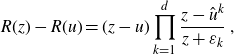 \begin{align}R(z)-R(u)=(z-u) \prod_{k=1}^d \frac{z-\hat{u}^k}{z+\varepsilon_k}\;,\end{align}
where
 $\hat{u}^k$
are the other preimages of R(u) under R.
$\hat{u}^k$
are the other preimages of R(u) under R.
Proof. Both sides are a rational function r(z), with zeros only in
 $u,\hat{u}^1,\dots,\hat{u}^d$
and poles only in
$u,\hat{u}^1,\dots,\hat{u}^d$
and poles only in
 $-\varepsilon_1,\dots,-\varepsilon_d,\infty$
, all of which are simple. So they differ by a constant factor, which has to be 1 because both sides satisfy
$-\varepsilon_1,\dots,-\varepsilon_d,\infty$
, all of which are simple. So they differ by a constant factor, which has to be 1 because both sides satisfy
 $\lim_{z\to\infty} {r(z)}/{z}=1$
.
$\lim_{z\to\infty} {r(z)}/{z}=1$
.
Proposition 4.6. With Ansatz 4.1 the two-point function is symmetric,
 $\mathcal{G}^{(0)}(z,w)=\mathcal{G}^{(0)}(w,z)$
. One has
$\mathcal{G}^{(0)}(z,w)=\mathcal{G}^{(0)}(w,z)$
. One has
 $\mathcal{G}^{(0)}(\varepsilon_k,\varepsilon_l)=\mathcal{G}_{kl}$
with
$\mathcal{G}^{(0)}(\varepsilon_k,\varepsilon_l)=\mathcal{G}_{kl}$
with
 $\mathcal{G}_{kl}$
given in (3.5).
$\mathcal{G}_{kl}$
given in (3.5).
Proof. Inserting (4.8) into (4.5) gives for
 $z,w\in \bigcup_{j=1}^d\mathcal{V}_j$
:
$z,w\in \bigcup_{j=1}^d\mathcal{V}_j$
:
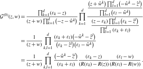 \begin{align}\mathcal{G}^{(0)}(z,w)&=\frac{\prod_{k=1}^d\!(\varepsilon_k-z)}{(z+w) \prod_{k=1}^d \!\big({-}z-\hat{w}^k\big)}\prod_{k=1}^d \frac{\displaystyle\frac{\big(z+\hat{w}^k\big)\prod_{l=1}^d \!\big({-}\hat{w}^k-\hat{z}^l\big)}{\prod_{l=1}^d \!\big(\varepsilon_l-\hat{w}^k\big)} }{\displaystyle \frac{(z-\varepsilon_k)\prod_{l=1}^d \!\big(\varepsilon_k-\hat{z}^l\big)}{\prod_{l=1}^d(\varepsilon_k+\varepsilon_l)}}\nonumber\\[-1ex]&= \frac{1}{(z+w)} \prod_{k,l=1}^d\frac{(\varepsilon_k+\varepsilon_l)\big({-}\hat{w}^k-\hat{z}^l\big)}{\big(\varepsilon_k-\hat{z}^l\big)\big(\varepsilon_l-\hat{w}^k\big)}\nonumber\\&= \frac{1}{(z+w)} \prod_{k,l=1}^d\frac{\big({-}\hat{w}^k-\hat{z}^l\big)}{(\varepsilon_k+\varepsilon_l)}\frac{(\varepsilon_k-z)}{(R(\varepsilon_k)-R(z))}\frac{(\varepsilon_l-w)}{(R(\varepsilon_l)-R(w))}\;.\end{align}
The limit
 $z\to \varepsilon_k$
and
$z\to \varepsilon_k$
and
 $w\to \varepsilon_l$
gives
$w\to \varepsilon_l$
gives
 $\mathcal{G}^{(0)}(\varepsilon_k,\varepsilon_l)=\mathcal{G}_{kl}$
.
$\mathcal{G}^{(0)}(\varepsilon_k,\varepsilon_l)=\mathcal{G}_{kl}$
.
We prove that (ii), (iv), (v), (vi) and (vii) of Ansatz 4.1 are automatic. We start with
Proposition 4.7. Relation (vii) of Ansatz 4.1 is consistent provided that
 $c_0=0$
.
$c_0=0$
.
Proof. With Lemma 4.4 and Lemma 4.3, both a consequence of Ansatz 4.1, each side of (4.1) is a rational function, and all poles are simple. For the term
 $ {r_k}/({R(\varepsilon_k)-R(z)})$
this follows from the assumption (ii) of Ansatz 4.1. We show that both sides of (4.1) have the same simple poles with the same residues. Then by Liouville’s theorem their difference is a constant, which is easy to control.
$ {r_k}/({R(\varepsilon_k)-R(z)})$
this follows from the assumption (ii) of Ansatz 4.1. We show that both sides of (4.1) have the same simple poles with the same residues. Then by Liouville’s theorem their difference is a constant, which is easy to control.
First, it follows from (4.7) and (4.5) that both sides of (4.1) approach z for
 $z\to \infty$
. Near
$z\to \infty$
. Near
 $\infty$
the difference between both sides of (4.1) is
$\infty$
the difference between both sides of (4.1) is
 $\pm 2c_0$
, which shows that
$\pm 2c_0$
, which shows that
 $c_0=0$
in (4.7) is necessary.
$c_0=0$
in (4.7) is necessary.
Next, (4.7) shows that the only other poles of the right-hand side of (4.1) are simple and located at
 $z=\varepsilon_k$
with residue
$z=\varepsilon_k$
with residue
 $-({\lambda}/{N}) \varrho_k$
. The same simple poles with the same residues are produced by
$-({\lambda}/{N}) \varrho_k$
. The same simple poles with the same residues are produced by
 $({\lambda}/{N}) \sum_{k=1}^d {r_k}/({R(\varepsilon_k)-R(z)})$
on the left-hand side, taking
$({\lambda}/{N}) \sum_{k=1}^d {r_k}/({R(\varepsilon_k)-R(z)})$
on the left-hand side, taking
 $r_k/R^{\prime}(\varepsilon_k)=\varrho_k$
into account.
$r_k/R^{\prime}(\varepsilon_k)=\varrho_k$
into account.
But the left-hand side of (4.1) could also have poles at
 $z=-\varepsilon_j$
and
$z=-\varepsilon_j$
and
 $z=\widehat{\varepsilon_m}^j$
(see (4.7) and (4.9)). We have
$z=\widehat{\varepsilon_m}^j$
(see (4.7) and (4.9)). We have
 $\textrm{Res}_{z= -\varepsilon_j}\ \ R(z)dz= - ({\lambda}/{N}) \varrho_j$
. Setting
$\textrm{Res}_{z= -\varepsilon_j}\ \ R(z)dz= - ({\lambda}/{N}) \varrho_j$
. Setting
 $w\mapsto \varepsilon_l$
in (4.5), then with
$w\mapsto \varepsilon_l$
in (4.5), then with
 $\lim_{z\to -\varepsilon_j} \big({R(z)-R\big({-}\widehat{\varepsilon_l}^k\big)}\big)/({ R(z)-R(\varepsilon_k)})=1$
for any k, l (here (v) of Ansatz 4.1 is used) one easily finds that
$\lim_{z\to -\varepsilon_j} \big({R(z)-R\big({-}\widehat{\varepsilon_l}^k\big)}\big)/({ R(z)-R(\varepsilon_k)})=1$
for any k, l (here (v) of Ansatz 4.1 is used) one easily finds that
 $\mathcal{G}^{(0)}({-}\varepsilon_j,\varepsilon_l)$
is finite for
$\mathcal{G}^{(0)}({-}\varepsilon_j,\varepsilon_l)$
is finite for
 $j\neq l$
and that
$j\neq l$
and that
 $\textrm{Res}_{z= -\varepsilon_j} ({\lambda}/{N})r_j\mathcal{G}^{(0)}\big(z,\varepsilon_j\big)dz= ({\lambda}/{N})\big({r_j}/{R^{\prime}\big(\varepsilon_j\big)}\big)$
, which thus cancels
$\textrm{Res}_{z= -\varepsilon_j} ({\lambda}/{N})r_j\mathcal{G}^{(0)}\big(z,\varepsilon_j\big)dz= ({\lambda}/{N})\big({r_j}/{R^{\prime}\big(\varepsilon_j\big)}\big)$
, which thus cancels
 $\textrm{Res}_{z= -\varepsilon_j} \ \ R(z)dz= -({\lambda}/{N}) \varrho_j$
.
$\textrm{Res}_{z= -\varepsilon_j} \ \ R(z)dz= -({\lambda}/{N}) \varrho_j$
.
Finally, from (4.5) we conclude
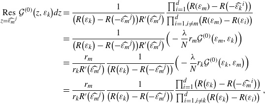 \begin{align*}\mathop{Res}\limits_{z= \widehat{\varepsilon_m}^j}\mathcal{G}^{(0)}\big(z,\varepsilon_k\big)dz&=\frac{1}{\big(R\big(\varepsilon_k\big)-R\big({-}\widehat{\varepsilon_m}^j\big)\big) R^{\prime}\big(\widehat{\varepsilon_m}^j\big)}\frac{\prod_{i=1}^d\!\big(R(\varepsilon_m)-R\big({-}\widehat{\varepsilon_k}^i\big)\big)}{\prod_{i=1,i\neq m }^d \!\big(R(\varepsilon_m)-R(\varepsilon_i)\big)}\\&=\frac{1}{\big(R\big(\varepsilon_k\big)-R\big({-}\widehat{\varepsilon_m}^j\big)\big) R^{\prime}\big(\widehat{\varepsilon_m}^j\big)}\Big( - \frac{\lambda}{N} r_m\mathcal{G}^{(0)}\big(\varepsilon_m,\varepsilon_k\big)\Big)\\&= \frac{r_m}{r_k R^{\prime}\big(\widehat{\varepsilon_m}^j\big)}\frac{1}{\big(R\big(\varepsilon_k\big)-R\big({-}\widehat{\varepsilon_m}^j\big)\big) }\Big( - \frac{\lambda}{N} r_k\mathcal{G}^{(0)}\big(\varepsilon_k,\varepsilon_m\big)\Big)\\&= \frac{r_m}{r_k R^{\prime}\big(\widehat{\varepsilon_m}^j\big)}\frac{1}{\big(R\big(\varepsilon_k\big)-R\big({-}\widehat{\varepsilon_m}^j\big)\big)}\frac{\prod_{i=1}^d\!\big(R\big(\varepsilon_k\big)-R\big({-}\widehat{\varepsilon_m}^i\big)\big)}{\prod_{i=1,i\neq k }^d \!\big(R\big(\varepsilon_k\big)-R(\varepsilon_i)\big)}\;,\end{align*}
where (4.4), the symmetry
 $\mathcal{G}^{(0)}(\varepsilon_m,\varepsilon_k)=\mathcal{G}^{(0)}(\varepsilon_k,\varepsilon_m)$
and again (4.4) have been used. The first identity (3.10) for
$\mathcal{G}^{(0)}(\varepsilon_m,\varepsilon_k)=\mathcal{G}^{(0)}(\varepsilon_k,\varepsilon_m)$
and again (4.4) have been used. The first identity (3.10) for
 $b_k=R(\varepsilon_k)$
and
$b_k=R(\varepsilon_k)$
and
 $a_j=R\big({-}\widehat{\varepsilon_m}^j\big)$
gives
$a_j=R\big({-}\widehat{\varepsilon_m}^j\big)$
gives
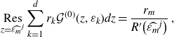 \begin{equation*}\mathop{Res}\limits_{z= \widehat{\varepsilon_m}^j}\sum_{k=1}^d r_k \mathcal{G}^{(0)}(z,\varepsilon_k)dz=\frac{r_m}{R^{\prime}\big(\widehat{\varepsilon_m}^j\big)}\;,\end{equation*}
which precisely cancels
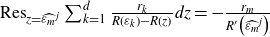 ${Res}_{z= \widehat{\varepsilon_m}^j}\sum_{k=1}^d\frac{r_k}{R(\varepsilon_k)-R(z)}dz= -\frac{r_m}{R^{\prime}\big(\widehat{\varepsilon_m}^j\big)}$
.
${Res}_{z= \widehat{\varepsilon_m}^j}\sum_{k=1}^d\frac{r_k}{R(\varepsilon_k)-R(z)}dz= -\frac{r_m}{R^{\prime}\big(\widehat{\varepsilon_m}^j\big)}$
.
Let us consider now the rational function
 \begin{equation}R(z)=z-\frac{\lambda}{N}\sum_{k=1}^d \frac{\varrho_k}{\varepsilon_k+z}\end{equation}
from equation (4.7) with
 $c_0=0$
. We are interested in the real and complex solutions
$c_0=0$
. We are interested in the real and complex solutions
 $\{\varepsilon_k,\varrho_k\}_{k=1,\dots,d}$
(depending on
$\{\varepsilon_k,\varrho_k\}_{k=1,\dots,d}$
(depending on
 $\lambda$
) of the 2d equations
$\lambda$
) of the 2d equations
 \begin{align}0&=R(\varepsilon_l)-E_l=\varepsilon_l -E_l -\frac{\lambda}{N}\sum_{k=1}^d \frac{\varrho_k}{\varepsilon_k+\varepsilon_l}\,=\!:\,\,f_l(\varepsilon_1,\varrho_1,\ldots,\varepsilon_d,\varrho_d,\lambda)\;,\end{align}
 \begin{align}0&= R^{\prime}(\varepsilon_l)- \frac{r_l}{\varrho_l}=1-\frac{r_l}{\varrho_l}+ \frac{\lambda}{N}\sum_{k=1}^d \frac{\varrho_k}{(\varepsilon_k+\varepsilon_l)^2}\,=\!:\,g_l(\varepsilon_1,\varrho_1,\ldots,\varepsilon_d,\varrho_d,\lambda)\end{align}
for
 $l=1,\dots,d$
from Theorem 3.1 for the given positive real numbers
$l=1,\dots,d$
from Theorem 3.1 for the given positive real numbers
 $E_l>0$
and
$E_l>0$
and
 $r_l>0$
from Section 2. In the following we only use that all these
$r_l>0$
from Section 2. In the following we only use that all these
 $E_l,r_l$
are positive (but not that
$E_l,r_l$
are positive (but not that
 $r_l$
is an integer counting the multiplicity of
$r_l$
is an integer counting the multiplicity of
 $E_l$
). So we consider for
$E_l$
). So we consider for
 $\mathbb{K}=\mathbb{R}$
or
$\mathbb{K}=\mathbb{R}$
or
 $\mathbb{K}=\mathbb{C}$
the real or complex algebraic subset
$\mathbb{K}=\mathbb{C}$
the real or complex algebraic subset
 \begin{equation*} Z(\mathbb{K})\,:\!=\,\{(\varepsilon_1,\varrho_1,\ldots,\varepsilon_d,\varrho_d,\lambda)\in U(\mathbb{K})|\: f_l=0,g_l=0,\: l=1,\dots,d\}\end{equation*}
in
 \begin{equation*}U(\mathbb{K})\,:\!=\,\{(\varepsilon_1,\varrho_1,\ldots,\varepsilon_d,\varrho_d,\lambda)|\:\varepsilon_k+\varepsilon_l\neq 0, \: \varrho_l\neq 0,\:k,l=1,\dots,d\}\subset \mathbb{K}^{2d+1}\:,\end{equation*}
i.e. in the complement of the corresponding central hyperplane arrangement in
 $\mathbb{K}^{2d+1}$
. Note that
$\mathbb{K}^{2d+1}$
. Note that
 $(\varepsilon_1,\varrho_1,\ldots,\varepsilon_d,\varrho_d,0)\in Z(\mathbb{K})$
iff
$(\varepsilon_1,\varrho_1,\ldots,\varepsilon_d,\varrho_d,0)\in Z(\mathbb{K})$
iff
 $\varepsilon_l=E_l$
and
$\varepsilon_l=E_l$
and
 $\varrho_l=r_l$
for all
$\varrho_l=r_l$
for all
 $l=1,\dots,d$
, and this real point belongs to the chamber
$l=1,\dots,d$
, and this real point belongs to the chamber
 \begin{equation*}U_{+}(\mathbb{R})\,:\!=\,\{(\varepsilon_1,\varrho_1,\ldots,\varepsilon_d,\varrho_d,\lambda)|\:\varepsilon_l > 0, \: \varrho_l > 0,\: l=1,\dots,d\}\subset U(\mathbb{R})\subset \mathbb{R}^{2d+1}\:.\end{equation*}
Note that the complex dimension of any irreducible component of
 $Z(\mathbb{C})$
is at least
$Z(\mathbb{C})$
is at least
 $1=(2d+1)-2d$
, since we are considering 2d equations in a Zariski-open subset of
$1=(2d+1)-2d$
, since we are considering 2d equations in a Zariski-open subset of
 $ \mathbb{C}^{2d+1}$
.
$ \mathbb{C}^{2d+1}$
.
Lemma 4.8.
 $Z(\mathbb{K})$
is a one-dimensional (real or complex) algebraic submanifold of
$Z(\mathbb{K})$
is a one-dimensional (real or complex) algebraic submanifold of
 $U(\mathbb{K})$
near the reference point
$U(\mathbb{K})$
near the reference point
 $(E_1,r_1,\ldots, E_d,r_d,0)$
, with the projection
$(E_1,r_1,\ldots, E_d,r_d,0)$
, with the projection
 \begin{equation*}pr\,:\, \mathbb{K}^{2d+1} \supset Z(\mathbb{K}) \longrightarrow \mathbb{K}\end{equation*}
onto the last
 $\lambda$
-coordinate a submersion near
$\lambda$
-coordinate a submersion near
 $(E_1,r_1,\ldots,E_d,r_d,0)$
in the Zariski topology. In particular, the reference point
$(E_1,r_1,\ldots,E_d,r_d,0)$
in the Zariski topology. In particular, the reference point
 $(E_1,r_1,\ldots, E_d,r_d,0)$
only belongs to one irreducible component of
$(E_1,r_1,\ldots, E_d,r_d,0)$
only belongs to one irreducible component of
 $Z(\mathbb{C})$
, which is of dimension one. Moreover, the map (of pointed sets)
$Z(\mathbb{C})$
, which is of dimension one. Moreover, the map (of pointed sets)
 \begin{equation*}pr\,:\, Z(\mathbb{K}) \longrightarrow \mathbb{K} \quad \text{ with} \quad pr(E_1,r_1,\ldots, E_d,r_d,0)=0\end{equation*}
becomes locally near
 $(E_1,r_1,\ldots, E_d,r_d,0)$
a (real or complex) analytic isomorphism onto an open interval or disc around
$(E_1,r_1,\ldots, E_d,r_d,0)$
a (real or complex) analytic isomorphism onto an open interval or disc around
 $\lambda=0\in \mathbb{K}$
, fitting with the description given in Theorem 3.1 in terms of the implicit function theorem.
$\lambda=0\in \mathbb{K}$
, fitting with the description given in Theorem 3.1 in terms of the implicit function theorem.
Proof. The claim follows from
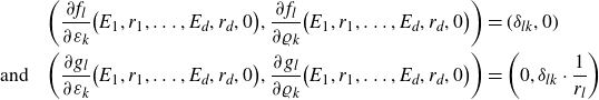 \begin{align*}\bigg(\frac{\partial f_l}{\partial \varepsilon_k}\big(E_1,r_1,\ldots, E_d,r_d,0\big), \frac{\partial f_l}{\partial \varrho_k}\big(E_1,r_1,\ldots, E_d,r_d,0\big)\bigg)&=(\delta_{lk},0)\\\text{and}\quad \bigg(\frac{\partial g_l}{\partial \varepsilon_k}\big(E_1,r_1,\ldots, E_d,r_d,0\big), \frac{\partial g_l}{\partial \varrho_k}\big(E_1,r_1,\ldots, E_d,r_d,0\big)\bigg)&=\bigg(0, \delta_{lk}\cdot \frac{1}{r_l}\bigg)\end{align*}
for
 $l,k=1,\dots,d$
.
$l,k=1,\dots,d$
.
Remark 4.9. Let us rewrite for a fixed
 $\lambda\in \mathbb{C}$
the equations (4.11) and (4.12) in terms of the d polynomials
$\lambda\in \mathbb{C}$
the equations (4.11) and (4.12) in terms of the d polynomials
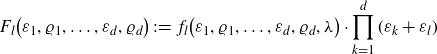 \begin{equation*}F_l\big(\varepsilon_1,\varrho_1,\ldots,\varepsilon_d,\varrho_d\big) \,:\!=\,f_l\big(\varepsilon_1,\varrho_1,\ldots,\varepsilon_d,\varrho_d,\lambda\big)\cdot \prod_{k=1}^d(\varepsilon_k+\varepsilon_l)\end{equation*}
of degree
 $d+1$
and the d polynomials
$d+1$
and the d polynomials
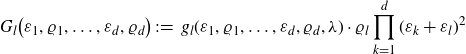 \begin{equation*}G_l\big(\varepsilon_1,\varrho_1,\ldots,\varepsilon_d,\varrho_d\big) \,:\!=\,g_l(\varepsilon_1,\varrho_1,\ldots,\varepsilon_d,\varrho_d,\lambda)\cdot\varrho_l \prod_{k=1}^d(\varepsilon_k+\varepsilon_l)^2\end{equation*}
of degree
 $2d+1$
(for
$2d+1$
(for
 $l=1,\dots,d$
), so that:
$l=1,\dots,d$
), so that:
 \begin{equation*}Z(\mathbb{C})\cap\{pr=\lambda\} \subset\big\{\big(\varepsilon_1,\varrho_1,\ldots,\varepsilon_d,\varrho_d\big)\in \mathbb{C}^{2d}|\: F_l=0,G_l=0,\: l=1,\dots,d\big\}\times\{\lambda\} \:.\end{equation*}
If for a given
 $\lambda\in \mathbb{C}$
the set
$\lambda\in \mathbb{C}$
the set
 \begin{equation*}\big\{\big(\varepsilon_1,\varrho_1,\ldots,\varepsilon_d,\varrho_d\big)\in \mathbb{C}^{2d}|\: F_l=0,G_l=0,\: l=1,\dots,d\big\}\end{equation*}
is finite, then one gets by the affine Bezout inequality [Reference Schmid29, Thm 3.1] the upper estimate
 $(d+1)^d(2d+1)^d$
for the number of solutions of the equations (4.11) and (4.12) (for this
$(d+1)^d(2d+1)^d$
for the number of solutions of the equations (4.11) and (4.12) (for this
 $\lambda$
).
$\lambda$
).
Let us come back to the rational function R(z) from (4.10) for the case of positive real
 $E_l>0$
and
$E_l>0$
and
 $r_l>0$
for
$r_l>0$
for
 $ l=1,\dots,d$
related to the solution of Theorem 3.1 as discussed before. Then
$ l=1,\dots,d$
related to the solution of Theorem 3.1 as discussed before. Then
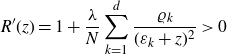 \begin{equation}R^{\prime}(z)=1+\frac{\lambda}{N}\sum_{k=1}^d \frac{\varrho_k}{(\varepsilon_k+z)^2}>0\end{equation}
for all
 $\lambda\geqslant 0$
and
$\lambda\geqslant 0$
and
 $z\in \mathbb{R}\backslash \{-\varepsilon_1,\dots,-\varepsilon_d\}$
.
$z\in \mathbb{R}\backslash \{-\varepsilon_1,\dots,-\varepsilon_d\}$
.
Lemma 4.10.
 $R^{-1}(E_k)$
consists for all
$R^{-1}(E_k)$
consists for all
 $E_k>0$
of
$E_k>0$
of
 $d+1$
different real points so that assumption (ii) of Ansatz 4.1 holds. Moreover we can choose
$d+1$
different real points so that assumption (ii) of Ansatz 4.1 holds. Moreover we can choose
 $\mathcal{U}=\mathcal{U}_1=\ldots=\mathcal{U}_d$
as a small simply connected open neighbourhood of
$\mathcal{U}=\mathcal{U}_1=\ldots=\mathcal{U}_d$
as a small simply connected open neighbourhood of
 $(R(0),\infty)\subset \mathbb{R}$
in
$(R(0),\infty)\subset \mathbb{R}$
in
 $\mathbb{C}$
, with
$\mathbb{C}$
, with
 $\mathcal{V}=\mathcal{V}_1= \ldots= \mathcal{V}_d$
also containing
$\mathcal{V}=\mathcal{V}_1= \ldots= \mathcal{V}_d$
also containing
 $(0,\infty)$
. By shrinking of
$(0,\infty)$
. By shrinking of
 $\mathcal{U}$
we can even assume that
$\mathcal{U}$
we can even assume that
 $\mathcal{V}\subset \{z\in \mathbb{C}|\;{Re}(z)>0\}$
. Then the assumptions (v) and (vi) of Ansatz 4.1 hold for all
$\mathcal{V}\subset \{z\in \mathbb{C}|\;{Re}(z)>0\}$
. Then the assumptions (v) and (vi) of Ansatz 4.1 hold for all
 $w\in \mathcal{V}$
with
$w\in \mathcal{V}$
with
 $\mathcal{V}$
small enough, as well as the assumption (iv) with
$\mathcal{V}$
small enough, as well as the assumption (iv) with
 $\mathcal{G}^{(0)}$
as in (4.5) resp. (4.9).
$\mathcal{G}^{(0)}$
as in (4.5) resp. (4.9).
Proof. If we order the numbering of the
 $\varepsilon_l$
as
$\varepsilon_l$
as
 $\varepsilon_i<\varepsilon_{i+1}$
for
$\varepsilon_i<\varepsilon_{i+1}$
for
 $i=0,\dots,d$
with
$i=0,\dots,d$
with
 $\varepsilon_0\,:\!=\,-\infty$
and
$\varepsilon_0\,:\!=\,-\infty$
and
 $\varepsilon_{d+1}\,:\!=\,+\infty$
, then
$\varepsilon_{d+1}\,:\!=\,+\infty$
, then
 \begin{equation*}R\,:\, ({-}\varepsilon_{i+1},-\varepsilon_i) \longrightarrow \mathbb{R}\end{equation*}
is for all
 $i=0,\dots,d$
strictly monotone increasing and bijective by the estimate
$i=0,\dots,d$
strictly monotone increasing and bijective by the estimate
 $R^{\prime}(z)>0$
above and the intermediate value theorem. This proves the first claim. Similarly,
$R^{\prime}(z)>0$
above and the intermediate value theorem. This proves the first claim. Similarly,
 $R^{-1}(R(w))$
consists for any
$R^{-1}(R(w))$
consists for any
 $w\in\mathcal{V}\cap (0,\infty)$
of
$w\in\mathcal{V}\cap (0,\infty)$
of
 $d+1$
real points which we can order as
$d+1$
real points which we can order as
 $\hat{w}^l\in ({-}\varepsilon_{l+1},-\varepsilon_l)$
. Therefore,
$\hat{w}^l\in ({-}\varepsilon_{l+1},-\varepsilon_l)$
. Therefore,
 $-\hat{w}^l\in (0,\infty)$
and all
$-\hat{w}^l\in (0,\infty)$
and all
 $R\big({-}\hat{w}^l\big)$
are distinct for
$R\big({-}\hat{w}^l\big)$
are distinct for
 $w\in\mathcal{V}\cap (0,\infty)$
, because R is injective on
$w\in\mathcal{V}\cap (0,\infty)$
, because R is injective on
 $({-}\varepsilon_1,\infty)$
. Moreover, R is an injective immersion in
$({-}\varepsilon_1,\infty)$
. Moreover, R is an injective immersion in
 $({-}\varepsilon_1,\infty)$
, which is an open condition so that also the second claim follows. Finally the assumption (iv) with
$({-}\varepsilon_1,\infty)$
, which is an open condition so that also the second claim follows. Finally the assumption (iv) with
 $\mathcal{G}^{(0)}$
as in (4.9) follows from
$\mathcal{G}^{(0)}$
as in (4.9) follows from
 $0\neq z+w$
for all
$0\neq z+w$
for all
 $z,w\in \mathcal{V}$
, since
$z,w\in \mathcal{V}$
, since
 $\textrm{Re}(z+w)=\textrm{Re}(z) +\textrm{Re}(w)>0$
.
$\textrm{Re}(z+w)=\textrm{Re}(z) +\textrm{Re}(w)>0$
.
We finish this section with the:
Proof of Theorem
3.1. We have seen that equation (3.2) can be solved by Ansatz 4.1 to
 $G^{(0)}(R(z),R(w))=\mathcal{G}^{(0)}(z,w)$
, where R is given in (4.10) and
$G^{(0)}(R(z),R(w))=\mathcal{G}^{(0)}(z,w)$
, where R is given in (4.10) and
 $\mathcal{G}^{(0)}$
in (4.5) resp. (4.9). This solution depends on the choice of preimages
$\mathcal{G}^{(0)}$
in (4.5) resp. (4.9). This solution depends on the choice of preimages
 $\varepsilon_k \in R^{-1}(E_k)$
made in (iv) of Ansatz 4.1. Any solution
$\varepsilon_k \in R^{-1}(E_k)$
made in (iv) of Ansatz 4.1. Any solution
 $\{\varepsilon_1,\dots, \varepsilon_d\}$
of the system of equations (3.3) provides a solution of (4.5), if also the assumptions (iv), (v) and (vi) of Ansatz 4.1 hold. Theorem 3.1 selects one particular solution of (3.2) which satisfies the assumptions (ii), (iv), (v) and (vi) of Ansatz 4.1 by Lemma 4.10. Hence also relation (vii) of Ansatz 4.1 holds by Proposition 4.7. The choice
$\{\varepsilon_1,\dots, \varepsilon_d\}$
of the system of equations (3.3) provides a solution of (4.5), if also the assumptions (iv), (v) and (vi) of Ansatz 4.1 hold. Theorem 3.1 selects one particular solution of (3.2) which satisfies the assumptions (ii), (iv), (v) and (vi) of Ansatz 4.1 by Lemma 4.10. Hence also relation (vii) of Ansatz 4.1 holds by Proposition 4.7. The choice
 $\lim_{\lambda\to 0}\varepsilon_k=E_k$
and
$\lim_{\lambda\to 0}\varepsilon_k=E_k$
and
 $\lim_{\lambda\to 0} \varrho_k=r_k$
is made to recover in the limit
$\lim_{\lambda\to 0} \varrho_k=r_k$
is made to recover in the limit
 $\lambda\to 0$
the moments of the Gaußian measure (2.1).
$\lambda\to 0$
the moments of the Gaußian measure (2.1).
It remains to show (3.4). On the right-hand side of (4.2) we use the the symmetry
 $\mathcal{G}^{(0)}(\varepsilon_k,w)=\mathcal{G}^{(0)}(w,\varepsilon_k)$
from Proposition 4.6 and express
$\mathcal{G}^{(0)}(\varepsilon_k,w)=\mathcal{G}^{(0)}(w,\varepsilon_k)$
from Proposition 4.6 and express
 $\mathcal{G}^{(0)}(w,\varepsilon_k)$
as (4.5) for
$\mathcal{G}^{(0)}(w,\varepsilon_k)$
as (4.5) for
 $w\mapsto \varepsilon_k$
and
$w\mapsto \varepsilon_k$
and
 $z\mapsto w$
. Dividing by
$z\mapsto w$
. Dividing by
 $(R(w)-R(z))$
gives
$(R(w)-R(z))$
gives
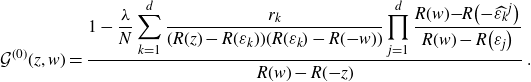 \begin{align}\mathcal{G}^{(0)}(z,w)=\frac{\displaystyle1 -\frac{\lambda}{N} \sum_{k=1}^d \frac{r_k}{(R(z)-R(\varepsilon_k))(R(\varepsilon_k)-R({-}w))}\prod_{j=1}^d \frac{R(w){-}R\big({-}\widehat{\varepsilon_k}^j\big)}{ R(w)-R\big(\varepsilon_j\big)}}{R(w)-R({-}z)}\;.\end{align}
This equation was obtained in [Reference Grosse, Hock and Wulkenhaar12] by another method. We rearrange it as
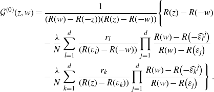 \begin{align*}\mathcal{G}^{(0)}(z,w)&=\frac{1}{(R(w)-R({-}z))(R(z)-R({-}w))}\Bigg\{R(z)-R({-}w)\\&\quad -\frac{\lambda}{N} \sum_{l=1}^d \frac{r_l}{(R(\varepsilon_l)-R({-}w))}\prod_{j=1}^d \frac{R(w)-R\big({-}\widehat{\varepsilon_l}^j\big)}{ R(w)-R\big(\varepsilon_j\big)}\\&\quad -\frac{\lambda}{N} \sum_{k=1}^d \frac{r_k}{(R(z)-R(\varepsilon_k))}\prod_{j=1}^d \frac{R(w)-R\big({-}\widehat{\varepsilon_k}^j\big)}{ R(w)-R\big(\varepsilon_j\big)}\Bigg\}\;.\end{align*}
The second line is
 $- ({\lambda}/{N}) \sum_{l=1}^d\mathcal{G}^{(0)}(w,\varepsilon_l)$
by (4.5). We combine it with the term
$- ({\lambda}/{N}) \sum_{l=1}^d\mathcal{G}^{(0)}(w,\varepsilon_l)$
by (4.5). We combine it with the term
 $-R({-}w)$
inside
$-R({-}w)$
inside
 $\{ \ \}$
according to our main algebraic relation (4.1). In the last line, the factor
$\{ \ \}$
according to our main algebraic relation (4.1). In the last line, the factor
 $\prod_{j=1}^d \!\big({R(w)-R\big({-}\widehat{\varepsilon_k}^j\big)}\big)/\big({ R(w)-R\big(\varepsilon_j\big)}\big)$
is rewitten via (4.6), with
$\prod_{j=1}^d \!\big({R(w)-R\big({-}\widehat{\varepsilon_k}^j\big)}\big)/\big({ R(w)-R\big(\varepsilon_j\big)}\big)$
is rewitten via (4.6), with
 $w\mapsto \varepsilon_k$
and
$w\mapsto \varepsilon_k$
and
 $z\mapsto w$
. We arrive at
$z\mapsto w$
. We arrive at
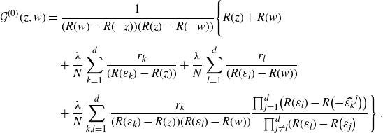 \begin{align*}\mathcal{G}^{(0)}(z,w)&=\frac{1}{(R(w)-R({-}z))(R(z)-R({-}w))}\Bigg\{R(z)+R(w)\\[4pt]& \quad +\frac{\lambda}{N} \sum_{k=1}^d \frac{r_k}{(R(\varepsilon_k)-R(z))}+\frac{\lambda}{N} \sum_{l=1}^d \frac{r_l}{(R(\varepsilon_l)-R(w))}\\[4pt]& \quad +\frac{\lambda}{N} \sum_{k,l=1}^d \frac{r_k}{(R(\varepsilon_k)-R(z))(R(\varepsilon_l)-R(w))}\frac{\prod_{j=1}^d\!\big(R(\varepsilon_l)-R\big({-}\widehat{\varepsilon_k}^j\big)\big)}{\prod_{j\neq l}^d \!(R(\varepsilon_l)-R\big(\varepsilon_j\big)}\Bigg\}\;.\end{align*}
The result (3.4) follows from equation (4.4) for
 $\mathcal{G}^{(0)}(\varepsilon_k,\varepsilon_l)$
.
$\mathcal{G}^{(0)}(\varepsilon_k,\varepsilon_l)$
.
5. The diagonal 2-point function
The diagonal planar cumulant
 $z\mapsto \mathcal{G}^{(0)}(z,z)$
of length 2 and cycle type (0, 1) admits a simpler formula due to properties of the rational function
$z\mapsto \mathcal{G}^{(0)}(z,z)$
of length 2 and cycle type (0, 1) admits a simpler formula due to properties of the rational function
 $\tilde{R}$
with
$\tilde{R}$
with
 $\tilde{R}(z)\,:\!=\,R(z)-R({-}z)$
. Let
$\tilde{R}(z)\,:\!=\,R(z)-R({-}z)$
. Let
 $z\in \big\{0,\pm \alpha_1,\dots, \pm \alpha_d\big\}$
be the list of roots of
$z\in \big\{0,\pm \alpha_1,\dots, \pm \alpha_d\big\}$
be the list of roots of
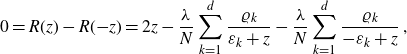 \begin{equation*}0= R(z)-R({-}z)=2z -\frac{\lambda}{N}\sum_{k=1}^d \frac{\varrho_k}{\varepsilon_k+z} -\frac{\lambda}{N}\sum_{k=1}^d \frac{\varrho_k}{-\varepsilon_k+z} \:,\end{equation*}
with the convention
 $\alpha_k>0$
and
$\alpha_k>0$
and
 $\alpha_k\neq \alpha_l$
for
$\alpha_k\neq \alpha_l$
for
 $k\neq l$
. Since here all
$k\neq l$
. Since here all
 $\varepsilon_k>0$
and
$\varepsilon_k>0$
and
 $\varrho_k>0$
are positive real numbers, we can argue as for the rational function R that also the rational function
$\varrho_k>0$
are positive real numbers, we can argue as for the rational function R that also the rational function
 $\tilde{R}$
maps each of the
$\tilde{R}$
maps each of the
 $2d+1$
connected components of
$2d+1$
connected components of
 $\mathbb{R}\backslash\{\pm\varepsilon_1, \dots, \pm \varepsilon_d\}$
bijectively onto
$\mathbb{R}\backslash\{\pm\varepsilon_1, \dots, \pm \varepsilon_d\}$
bijectively onto
 $\mathbb{R}$
. So the odd function
$\mathbb{R}$
. So the odd function
 $\tilde{R}$
has indeed
$\tilde{R}$
has indeed
 $2d+1$
different real roots
$2d+1$
different real roots
 $\big\{0,\pm \alpha_1,\dots, \pm \alpha_d\big\}$
of the equation
$\big\{0,\pm \alpha_1,\dots, \pm \alpha_d\big\}$
of the equation
 $\tilde{R}=0$
. Taking its poles
$\tilde{R}=0$
. Taking its poles
 $\{\infty,\pm \varepsilon_k\}$
into account, we have
$\{\infty,\pm \varepsilon_k\}$
into account, we have
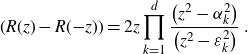 \begin{align}(R(z)-R({-}z))&= 2z \prod_{k=1}^d \frac{\big(z^2-\alpha_k^2\big)}{\big(z^2-\varepsilon_k^2\big)}\;.\end{align}
Proposition 5.1. For any
 $z\in \hat{\mathbb{C}}$
, the diagonal planar cumulant of cycle type
$z\in \hat{\mathbb{C}}$
, the diagonal planar cumulant of cycle type
 $(0, 1)$
can be simplified to
$(0, 1)$
can be simplified to
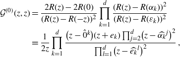 \begin{align}\mathcal{G}^{(0)}(z,z)&=\frac{2 R(z)-2R(0)}{(R(z)-R({-}z))^2}\prod_{k=1}^d \frac{(R(z)-R(\alpha_k))^2}{(R(z)-R(\varepsilon_k))^2}\\[-2pt]&\equiv \frac{1}{2z} \prod_{k=1}^d\frac{\big(z-\hat{0}^k\big)(z+e_k)\prod_{j=2}^d \!\big(z-\widehat{\alpha_k}^j\big)^2}{\prod_{l=1}^d \!\big(z-\widehat{e_k}^l\big)^2}\;,\nonumber\end{align}
in the convention
 $\widehat{\alpha_k}^1\equiv -\alpha_k$
.
$\widehat{\alpha_k}^1\equiv -\alpha_k$
.
Proof. The
 $d+1$
fold product of (5.1) for
$d+1$
fold product of (5.1) for
 $\big\{z,\hat{z}^1,\dots,\hat{z}^d\big\}$
is inserted into (4.5):
$\big\{z,\hat{z}^1,\dots,\hat{z}^d\big\}$
is inserted into (4.5):
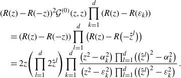 \begin{align}&(R(z)-R({-}z))^2 \mathcal{G}^{(0)}(z,z) \prod_{k=1}^d(R(z)-R(\varepsilon_k))\nonumber\\[-2ex]& \quad = (R(z)-R({-}z))\prod_{l=1}^d\big(R(z)-R\big({-}\hat{z}^l\big)\big) \nonumber\\[-1ex]& \quad = 2z\Bigg(\prod_{l=1}^d 2\hat{z}^l\Bigg)\prod_{k=1}^d \frac{\big(z^2-\alpha_k^2\big)\prod_{l=1}^d \!\big(\big(\hat{z}^l\big)^2-\alpha_k^2\big)}{\big(z^2-\varepsilon_k^2\big)\prod_{l=1}^d \!\big(\big(\hat{z}^l\big)^2-\varepsilon_k^2\big)}\;.\end{align}
We use cases of (4.8); the third one takes
 $R(\alpha_k)=R({-}\alpha_k)$
into account:
$R(\alpha_k)=R({-}\alpha_k)$
into account:
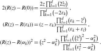 \begin{align*}2(R(z)-R(0))&=\frac{2z\prod_{l=1}^d \!\big(2\hat{z}_l\big) }{\prod_{k=1}^d \!\big({-}2\varepsilon_k\big)}\;,\\[-0.5ex](R(z)-R(\varepsilon_k))&=(z-\varepsilon_k)\frac{\prod_{l=1}^d \!\big(\varepsilon_k-\hat{z}^l\big) }{\prod_{l=1}^d \!(\varepsilon_k+\varepsilon_l)}\;,\\(R(z)-R(\alpha_k))^2&=\big(z^2-\alpha_k^2\big)\frac{\prod_{l=1}^d \!\big(\big(\hat{z}^l\big)^2-\alpha_k^2\big) }{\prod_{l=1}^d \!\big(\varepsilon_l^2-\alpha_k^2\big)}\;.\end{align*}
We identify in (5.3) the first equation and the product over k of the second and third equations:
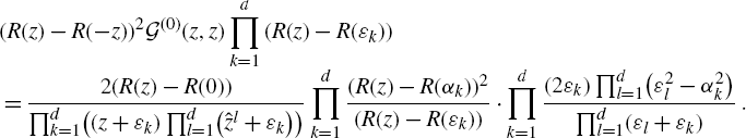 \begin{align*}&(R(z)-R({-}z))^2 \mathcal{G}^{(0)}(z,z) \prod_{k=1}^d(R(z)-R(\varepsilon_k))\nonumber\\&= \frac{2(R(z)-R(0))}{\prod_{k=1}^d \!\big((z+\varepsilon_k)\prod_{l=1}^d \!\big(\hat{z}^l+\varepsilon_k\big)\big)}\prod_{k=1}^d\frac{(R(z)-R(\alpha_k))^2}{(R(z)-R(\varepsilon_k))}\cdot \prod_{k=1}^d \frac{(2\varepsilon_k)\prod_{l=1}^d \!\big(\varepsilon_l^2-\alpha_k^2\big)}{\prod_{l=1}^d \!(\varepsilon_l+\varepsilon_k)}\;.\end{align*}
Now observe that the residue of (4.8) at
 $z=-\varepsilon_k$
is the identity
$z=-\varepsilon_k$
is the identity
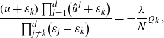 \begin{align}\frac{(u+\varepsilon_k)\prod_{l=1}^d\!\big(\hat{u}^l+\varepsilon_k\big)}{\prod_{j\neq k}^d\!\big(\varepsilon_j-\varepsilon_k\big)} = -\frac{\lambda}{N} \varrho_k\;,\end{align}
for any
 $u\notin R^{-1}(\{\infty\})$
. Consequently,
$u\notin R^{-1}(\{\infty\})$
. Consequently,
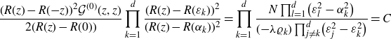 \begin{align*}\frac{(R(z)-R({-}z))^2 \mathcal{G}^{(0)}(z,z)}{2(R(z)-R(0))}\prod_{k=1}^d\frac{(R(z)-R(\varepsilon_k))^2}{(R(z)-R(\alpha_k))^2}&= \prod_{k=1}^d \frac{ N\prod_{l=1}^d \!\big(\varepsilon_l^2-\alpha_k^2\big)}{({-}\lambda\varrho_k)\prod_{j\neq k}^d\!\big(\varepsilon_j^2-\varepsilon_k^2\big)}=C\end{align*}
is a constant independent of z, which for
 $z\to \infty$
is identified as
$z\to \infty$
is identified as
 $C=1$
.
$C=1$
.
The following result will be needed in the next section:
Lemma 5.2. For any
 $w\in \hat{\mathbb{C}}$
one has
$w\in \hat{\mathbb{C}}$
one has
 \begin{align}\frac{1}{R(w)-R({-}w)}+ \sum_{k=1}^d\frac{1}{R(w)-R\big({-}\hat{w}^k\big)}&=\frac{1}{2(R(w){-}R(0))}+\sum_{k=1}^d \frac{1}{R(w)-R(\alpha_k)}\;.\end{align}
Proof. Taking
 $R(w)=R\big(\hat{w}^k\big)$
into account, all terms on the lhs of (5.5) are of the form (5.1) so that the lhs of (5.5) has simple poles at
$R(w)=R\big(\hat{w}^k\big)$
into account, all terms on the lhs of (5.5) are of the form (5.1) so that the lhs of (5.5) has simple poles at
 $w \in \{0,\pm \alpha_l\}$
and
$w \in \{0,\pm \alpha_l\}$
and
 $\hat{w}^k\in \{0,\pm\alpha_l\}$
. Applying R shows that these
$\hat{w}^k\in \{0,\pm\alpha_l\}$
. Applying R shows that these
 $\hat{w}^k$
correspond to additional poles at
$\hat{w}^k$
correspond to additional poles at
 $w \in \big\{\hat{0}^l, \widehat{\alpha_l}^j,\mp\alpha_l\big\}$
for
$w \in \big\{\hat{0}^l, \widehat{\alpha_l}^j,\mp\alpha_l\big\}$
for
 $l=1,\dots,d$
and
$l=1,\dots,d$
and
 $j=2,\dots,d$
. We evaluate the residues at these poles and check that the rhs of (5.5) has the same poles (clear) with the same residues.
$j=2,\dots,d$
. We evaluate the residues at these poles and check that the rhs of (5.5) has the same poles (clear) with the same residues.
Note that
 $R(w)=R\big(\hat{w}^k\big)$
implies
$R(w)=R\big(\hat{w}^k\big)$
implies
 $R^{\prime}(w) =R^{\prime}\big(\hat{w}^k\big) \big(\hat{w}^k\big)^{\prime}(w)$
or
$R^{\prime}(w) =R^{\prime}\big(\hat{w}^k\big) \big(\hat{w}^k\big)^{\prime}(w)$
or
 $\big(\hat{w}^k\big)^{\prime}(w)= {R^{\prime}(w)}/{R^{\prime}\big(\hat{w}^k\big)}$
. Consider the pole at
$\big(\hat{w}^k\big)^{\prime}(w)= {R^{\prime}(w)}/{R^{\prime}\big(\hat{w}^k\big)}$
. Consider the pole at
 $w=\pm \alpha_l$
. Then there is precisely one
$w=\pm \alpha_l$
. Then there is precisely one
 $k_l\in \{1,\dots, d\}$
with
$k_l\in \{1,\dots, d\}$
with
 $\hat{w}^{k_l}=\mp \alpha_l$
. Therefore,
$\hat{w}^{k_l}=\mp \alpha_l$
. Therefore,
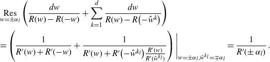 \begin{align*}&\mathop{Res}\limits_{w= \pm \alpha_l}\Bigg(\frac{dw }{R(w)-R({-}w)}+ \sum_{k=1}^d\frac{dw}{R(w)-R\big({-}\hat{w}^k\big)}\Bigg)\nonumber\\&= \left(\frac{1}{R^{\prime}(w)+R^{\prime}({-}w)}+\frac{1}{R^{\prime}(w)+R^{\prime}\big({-}\hat{w}^{k_l}\big)\frac{R^{\prime}(w)}{R^{\prime}(\hat{w}^{k_l})}}\right)\Bigg|_{w=\pm \alpha_l,\hat{w}^{k_l}=\mp\alpha_l}=\frac{1}{R^{\prime}(\!\pm \alpha_l)}\;.\end{align*}
Consider in case of
 $d\geqslant 2$
the pole at
$d\geqslant 2$
the pole at
 $w=\widehat{\alpha_l}^j$
. There are precisely two distinct
$w=\widehat{\alpha_l}^j$
. There are precisely two distinct
 $k_+,k_- \in \{1,\dots, d\}$
with
$k_+,k_- \in \{1,\dots, d\}$
with
 $\hat{w}^{k_+}=\alpha_l$
and
$\hat{w}^{k_+}=\alpha_l$
and
 $\hat{w}^{k_-}=-\alpha_l$
. Therefore,
$\hat{w}^{k_-}=-\alpha_l$
. Therefore,
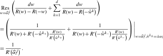 \begin{align*}&\mathop{Res}\limits_{w= \widehat{\alpha_l}^j}\Bigg(\frac{dw }{R(w)-R({-}w)}+ \sum_{k=1}^d\frac{dw}{R(w)-R\big({-}\hat{w}^k\big)}\Bigg)\nonumber\\&=\left(\frac{1}{R^{\prime}(w)+R^{\prime}\big({-}\hat{w}^{k_+}\big)\frac{R^{\prime}(w)}{R^{\prime}\big(\hat{w}^{k_+}\big)}}+\frac{1}{R^{\prime}(w)+R^{\prime}\big({-}\hat{w}^{k_-}\big)\frac{R^{\prime}(w)}{R^{\prime}\big(\hat{w}^{k_-}\big)}}\right)\Bigg|_{w=\widehat{\alpha_l}^j,\hat{w}^{k_\pm}=\pm\alpha_l}\\&=\frac{1}{R^{\prime}\big(\widehat{\alpha_l}^j\big)}\;.\end{align*}
The rhs of (5.5) has exactly the same residues.
Finally, it is also clear that both sides of (5.5) have the same residue
 ${1}/{2R^{\prime}(0)}$
at
${1}/{2R^{\prime}(0)}$
at
 $w=0$
. For
$w=0$
. For
 $w=\hat{0}^l$
there is a unique
$w=\hat{0}^l$
there is a unique
 $k_l \in \{1,\dots, d\}$
with
$k_l \in \{1,\dots, d\}$
with
 $\hat{w}^{k_l}=0$
. Then
$\hat{w}^{k_l}=0$
. Then
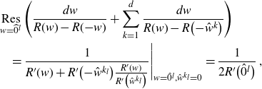 \begin{align*}&\mathop{Res}\limits_{w= \widehat{0}^l}\Bigg(\frac{dw }{R(w)-R({-}w)}+ \sum_{k=1}^d\frac{dw}{R(w)-R\big({-}\hat{w}^k\big)}\Bigg)\nonumber\\& \quad = \frac{1}{R^{\prime}(w)+R^{\prime}\big({-}\hat{w}^{k_l}\big)\frac{R^{\prime}(w)}{R^{\prime}\big(\hat{w}^{k_l}\big)}}\Bigg|_{w=\hat{0}^l,\hat{w}^{k_l}=0}=\frac{1}{2R^{\prime}\big(\hat{0}^l\big)}\;,\end{align*}
which agrees with the residue of the rhs of (5.5). Therefore, the difference between lhs and rhs of (5.5) is a bounded entire function, i.e. a constant by Liouville’s theorem, which is zero when considering
 $w\to \infty$
. This completes the proof.
$w\to \infty$
. This completes the proof.
6. The planar
$1+1$
-point function

The
 $1+1$
-point function
$1+1$
-point function
 $G_{|a|b|}$
is the cumulant of length 2 and cycle type (2, 0) (i.e. two cycles a and b of length 1), see Appendix A. We derive in Appendix B its equation of motion (B8) whose restriction to the planar sector (of degree or genus
$G_{|a|b|}$
is the cumulant of length 2 and cycle type (2, 0) (i.e. two cycles a and b of length 1), see Appendix A. We derive in Appendix B its equation of motion (B8) whose restriction to the planar sector (of degree or genus
 $g=0$
) reads
$g=0$
) reads
 \begin{align}(E_a+E_a)G_{|a|b|}^{(0)} &=-\frac{\lambda}{N}\sum_{k=1}^{N} G^{(0)}_{|ak|}G^{(0)}_{|a|b|}+\frac{\lambda}{N}\sum_{k=1}^{N}\frac{G^{(0)}_{|k|b|}-G^{(0)}_{|a|b|}}{E_k-E_a}+\lambda\frac{G^{(0)}_{|bb|}-G^{(0)}_{|ab|}}{E_b-E_a}\;.\end{align}
We interpret this equation as evaluation
 $G_{|a|b|}^{(0)}=\mathcal{G}^{(0)}(\varepsilon_a|\varepsilon_b)$
of a functionFootnote 2
$G_{|a|b|}^{(0)}=\mathcal{G}^{(0)}(\varepsilon_a|\varepsilon_b)$
of a functionFootnote 2
 $\mathcal{G}^{(0)}(z|w)$
which satisfies
$\mathcal{G}^{(0)}(z|w)$
which satisfies
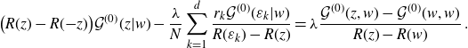 \begin{align}\big( R(z)-R({-}z)\big) \mathcal{G}^{(0)}(z|w)- \frac{\lambda}{N} \sum_{k=1}^d\frac{r_k\mathcal{G}^{(0)}(\varepsilon_k|w) }{R(\varepsilon_k)-R(z)}&=\lambda \frac{\mathcal{G}^{(0)}(z,w)-\mathcal{G}^{(0)}(w,w)}{R(z)-R(w)}\;.\end{align}
The identity (4.1) was decisive here, and multiplicities
 $r_k$
of the
$r_k$
of the
 $E_k=R(\varepsilon_k)$
were admitted.
$E_k=R(\varepsilon_k)$
were admitted.
Since
 $\mathcal{G}^{(0)}(\alpha_k|w)$
must be regularFootnote 3 for any
$\mathcal{G}^{(0)}(\alpha_k|w)$
must be regularFootnote 3 for any
 $w>0$
, evaluation at
$w>0$
, evaluation at
 $z=\alpha_k$
produces d equations
$z=\alpha_k$
produces d equations
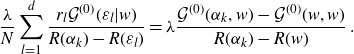 \begin{align}\frac{\lambda}{N} \sum_{l=1}^d\frac{r_l\mathcal{G}^{(0)}(\varepsilon_l|w) }{R(\alpha_k)-R(\varepsilon_l)}&=\lambda \frac{\mathcal{G}^{(0)}(\alpha_k,w)-\mathcal{G}^{(0)}(w,w)}{R(\alpha_k)-R(w)}\;.\end{align}
Equation (6.3) is with Proposition 3.2 solved by
 \begin{align*}\frac{r_k}{N} \mathcal{G}^{(0)}(\varepsilon_k|w)=\sum_{l=1}^{d}(R(\alpha_l)-R(\varepsilon_k)) \textbf{A}_l(R(\varepsilon_k))\textbf{E}_k(R(\alpha_l))\frac{\mathcal{G}^{(0)}(\alpha_l,w)-\mathcal{G}^{(0)}(w,w)}{R(\alpha_l)-R(w)}\;,\end{align*}
where
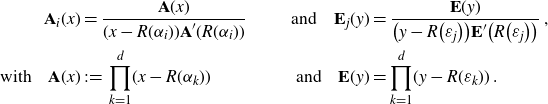 \begin{align*}\textbf{A}_i(x)&=\frac{\textbf{A}(x)}{(x-R(\alpha_i))\textbf{A}^{\prime}(R(\alpha_i))}&\text{and} \quad \textbf{E}_j(y)&=\frac{\textbf{E}(y)}{\big(y-R\big(\varepsilon_j\big)\big)\textbf{E}^{\prime}\big(R\big(\varepsilon_j\big)\big)}\:,\\\text{with}\quad \textbf{A}(x)&\,:\!=\,\prod_{k=1}^d \!(x-R(\alpha_k)) & \text{and} \quad \textbf{E}(y)&=\prod_{k=1}^d \!(y-R(\varepsilon_k)) \:.\end{align*}
Here, the
 $R(\alpha_k)$
and
$R(\alpha_k)$
and
 $R(\varepsilon_l)$
are pairwise distinct, since R is injective on
$R(\varepsilon_l)$
are pairwise distinct, since R is injective on
 $({-}\varepsilon_1,\infty)$
. Inserting this back into (6.2) gives the
$({-}\varepsilon_1,\infty)$
. Inserting this back into (6.2) gives the
 $1+1$
-point function
$1+1$
-point function
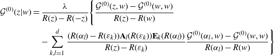 \begin{align}\mathcal{G}^{(0)}(z|w)&= \frac{\lambda}{R(z)-R({-}z)}\Bigg\{\frac{\mathcal{G}^{(0)}(z,w)-\mathcal{G}^{(0)}(w,w)}{R(z)-R(w)}\nonumber\\&\quad -\sum_{k,l=1}^{d}\frac{(R(\alpha_l)-R(\varepsilon_k)) \textbf{A}_l(R(\varepsilon_k))\textbf{E}_k(R(\alpha_l)) }{R(z)-R(\varepsilon_k)}\frac{\mathcal{G}^{(0)}(\alpha_l,w)-\mathcal{G}^{(0)}(w,w)}{R(\alpha_l)-R(w)}\Bigg\}\end{align}
in terms of the 2-point function
 $\mathcal{G}^{(0)}(z,w)$
known from Theorem 3.1. We convert the solution (6.4) into a manifestly symmetric form:
$\mathcal{G}^{(0)}(z,w)$
known from Theorem 3.1. We convert the solution (6.4) into a manifestly symmetric form:
Proposition 6.1. The planar cumulant of length 2 and cycle type (2, 0) has the solution
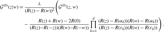 \begin{align}\mathcal{G}^{(0)}(z|w)&= \frac{\lambda}{(R(z)-R(w))^2} \Bigg(\mathcal{G}^{(0)}(z,w)\\&\quad -\frac{R(z)+R(w)-2R(0)}{(R(z){-}R({-}z))(R(w){-}R({-}w))}\prod_{k=1}^d \frac{(R(z)-R(\alpha_k))(R(w)-R(\alpha_k))}{(R(z)-R(\varepsilon_k))(R(w)-R(\varepsilon_k))}\Bigg)\,.\nonumber\end{align}
Proof. Using (3.8) we evaluate the k-sum in (6.4) to
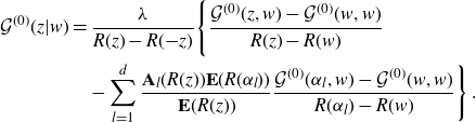 \begin{align}\mathcal{G}^{(0)}(z|w)&= \frac{\lambda}{R(z)-R({-}z)}\Bigg\{\frac{\mathcal{G}^{(0)}(z,w)-\mathcal{G}^{(0)}(w,w)}{R(z)-R(w)}\nonumber\\&\quad -\sum_{l=1}^{d}\frac{\textbf{A}_l(R(z))\textbf{E}(R(\alpha_l))}{\textbf{E}(R(z))}\frac{\mathcal{G}^{(0)}(\alpha_l,w)-\mathcal{G}^{(0)}(w,w)}{R(\alpha_l)-R(w)}\Bigg\}\;.\end{align}
In the second line we have
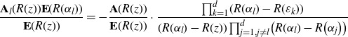 \begin{equation*}\frac{\textbf{A}_l(R(z))\textbf{E}(R(\alpha_l))}{\textbf{E}(R(z))}=-\frac{\textbf{A}(R(z))}{\textbf{E}(R(z))}\cdot \frac{\prod_{k=1}^d \!(R(\alpha_l)-R(\varepsilon_k))}{(R(\alpha_l)-R(z))\prod_{j=1,j\neq l}^d \!\big(R(\alpha_l)-R\big(\alpha_j\big)\big)}\end{equation*}
and we recall
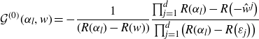 \begin{equation*}\mathcal{G}^{(0)}(\alpha_l,w)=-\frac{1}{(R(\alpha_l)-R(w))}\frac{\prod_{j=1}^d R(\alpha_l)-R\big({-}\hat{w}^j\big)}{\prod_{j=1}^d \!\big(R(\alpha_l)-R\big(\varepsilon_j\big)\big)}\end{equation*}
from (4.5). Inserting both identities into (6.6) gives after a first partial fraction decomposition
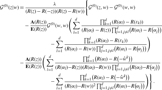 \begin{align}\mathcal{G}^{(0)}(z|w)&= \frac{\lambda}{(R(z)-R({-}z))(R(z)-R(w))}\Bigg\{\mathcal{G}^{(0)}(z,w)-\mathcal{G}^{(0)}(w,w)\nonumber\\&\quad -\frac{\textbf{A}(R(z))}{\textbf{E}(R(z))}\mathcal{G}^{(0)}(w,w)\Bigg(\sum_{l=1}^{d}\frac{\prod_{k=1}^d \!(R(\alpha_l)-R(\varepsilon_k))}{(R(\alpha_l)-R(z))\prod_{j=1,j\neq l}^d \!\big(R(\alpha_l)-R\big(\alpha_j\big)\big)}\nonumber\\&\qquad \qquad \qquad -\sum_{l=1}^{d} \frac{\prod_{k=1}^d \!(R(\alpha_l)-R(\varepsilon_k))}{(R(\alpha_l)-R(w))\prod_{j=1,j\neq l}^d \!\big(R(\alpha_l)-R\big(\alpha_j\big)\big)}\Bigg)\nonumber\\&-\frac{\textbf{A}(R(z))}{\textbf{E}(R(z))}\Bigg(\sum_{l=1}^{d}\frac{\prod_{k=1}^d \!\big(R(\alpha_l)-R\big({-}\hat{w}^k\big)\big)}{(R(\alpha_l){-}R(z))(R(\alpha_l){-}R(w))\prod_{j=1,j\neq l}^d \!\big(R(\alpha_l){-}R\big(\alpha_j\big)\big)}\nonumber\\&\qquad \qquad \qquad -\sum_{l=1}^{d}\frac{\prod_{k=1}^d \!\big(R(\alpha_l)-R\big({-}\hat{w}^k\big)\big)}{(R(\alpha_l){-}R(w))^2\prod_{j=1,j\neq l}^d \!\big(R(\alpha_l){-}R\big(\alpha_j\big)\big)}\Bigg)\Bigg\}\,.\end{align}
The second and third line are converted via an identity (4.6) with substitution
 $\varepsilon_i\mapsto \alpha_i$
and
$\varepsilon_i\mapsto \alpha_i$
and
 $-\hat{w}^j\mapsto\varepsilon_j$
. One of the surviving terms cancels
$-\hat{w}^j\mapsto\varepsilon_j$
. One of the surviving terms cancels
 $\mathcal{G}^{(0)}(w,w)$
in the first line of (6.7). Another partial fraction decomposition in the fourth line of (6.7) and
$\mathcal{G}^{(0)}(w,w)$
in the first line of (6.7). Another partial fraction decomposition in the fourth line of (6.7) and
 ${1}/({(R(\alpha_l)-R(w))^2})=\lim_{u\to w} {1}/({(R(u)-R(w))})\big({1}/({(R(\alpha_l)-R(u))})- {1}/({(R(\alpha_l)-R(w))}))$
in the fifth line of (6.7) also give rise to expressions (4.6) with substitution
${1}/({(R(\alpha_l)-R(w))^2})=\lim_{u\to w} {1}/({(R(u)-R(w))})\big({1}/({(R(\alpha_l)-R(u))})- {1}/({(R(\alpha_l)-R(w))}))$
in the fifth line of (6.7) also give rise to expressions (4.6) with substitution
 $\varepsilon_i\mapsto \alpha_i$
. We thus find
$\varepsilon_i\mapsto \alpha_i$
. We thus find
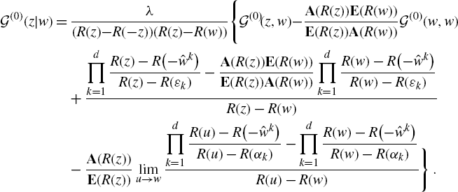 \begin{align*}\mathcal{G}^{(0)}(z|w)& = \frac{\lambda}{(R(z){-}R({-}z))(R(z){-}R(w))} \Bigg\{\mathcal{G}^{(0)}\:\!\!(z,w){-}\frac{\textbf{A}(R(z))\textbf{E}(R(w))}{\textbf{E}(R(z))\textbf{A}(R(w))}\mathcal{G}^{(0)}\:\!(w,w)\nonumber\\& \quad +\frac{\displaystyle\prod_{k=1}^{d}\frac{R(z)-R\big({-}\hat{w}^k\big)}{R(z)-R(\varepsilon_k)}-\frac{\textbf{A}(R(z))\textbf{E}(R(w))}{\textbf{E}(R(z))\textbf{A}(R(w))}\prod_{k=1}^{d}\frac{R(w)-R\big({-}\hat{w}^k\big)}{R(w)-R(\varepsilon_k)}}{R(z)-R(w)}\nonumber\\& \quad -\frac{\textbf{A}(R(z))}{\textbf{E}(R(z))}\lim_{u\to w}\frac{\displaystyle\prod_{k=1}^{d}\frac{R(u)-R\big({-}\hat{w}^k\big)}{R(u)-R(\alpha_k)}-\prod_{k=1}^{d}\frac{R(w)-R\big({-}\hat{w}^k\big)}{R(w)-R(\alpha_k)}}{R(u)-R(w)}\Bigg\}\;.\end{align*}
After evaluation of the limit we reconstruct in the last two lines
 $\mathcal{G}^{(0)}(z,w)$
and
$\mathcal{G}^{(0)}(z,w)$
and
 $\mathcal{G}^{(0)}(w,w)$
via (4.5):
$\mathcal{G}^{(0)}(w,w)$
via (4.5):
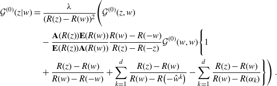 \begin{align*}\mathcal{G}^{(0)}(z|w)&= \frac{\lambda}{(R(z)-R(w))^2} \Bigg(\mathcal{G}^{(0)}(z,w)\nonumber\\& \quad -\frac{\textbf{A}(R(z))\textbf{E}(R(w))}{\textbf{E}(R(z))\textbf{A}(R(w))}\frac{R(w)-R({-}w)}{R(z)-R({-}z)}\mathcal{G}^{(0)}(w,w)\Bigg\{1 \nonumber\\& \quad +\frac{R(z)-R(w)}{R(w)-R({-}w)}+\sum_{k=1}^d \frac{R(z)-R(w)}{R(w)-R\big({-}\hat{w}^k\big)}- \sum_{k=1}^d\frac{R(z)-R(w)}{R(w)-R(\alpha_k)}\Bigg\}\Bigg)\;.\end{align*}
With Lemma 5.2 the terms in
 $\{ \ \}$
can be reduced to
$\{ \ \}$
can be reduced to
 $\{ \ \}= ({R(z)+R(w)-2R(0)})/$
 $({2(R(w)-R(0))})$
. Inserting (5.2) for
$({2(R(w)-R(0))})$
. Inserting (5.2) for
 $\mathcal{G}^{(0)}(w,w)$
gives the final result (6.5).
$\mathcal{G}^{(0)}(w,w)$
gives the final result (6.5).
7. Outlook
We have developed a new algebraic solution strategy for the two initial cumulants of a quartic analogue of the Kontsevich model. Our results have been extended in [Reference Branahl, Hock and Wulkenhaar3] to an algorithm which allows to recursively compute all other cumulants. The key discovery of [Reference Branahl, Hock and Wulkenhaar3] was to understand that one first has to focus on three families
 $\Omega^{(g)}_{m}(u_1,...,u_m)$
,
$\Omega^{(g)}_{m}(u_1,...,u_m)$
,
 $\mathcal{T}^{(g)}(u_1,...,u_m\|z,w|)$
and
$\mathcal{T}^{(g)}(u_1,...,u_m\|z,w|)$
and
 $\mathcal{T}^{(g)}(u_1,...,u_m\|z|w|)$
of auxiliary functions. Their simplest cases are the functions
$\mathcal{T}^{(g)}(u_1,...,u_m\|z|w|)$
of auxiliary functions. Their simplest cases are the functions
 $\mathcal{T}^{(0)}(\emptyset \|z,w|)\,:\!=\,\mathcal{G}^{(0)}(z,w)$
and
$\mathcal{T}^{(0)}(\emptyset \|z,w|)\,:\!=\,\mathcal{G}^{(0)}(z,w)$
and
 $\mathcal{T}^{(0)}(\emptyset \|z|w|)\,:\!=\,\mathcal{G}^{(0)}(z|w)$
analysed in this paper. The auxiliary functions are special polynomials [Reference Branahl, Hock and Wulkenhaar2] in the original cumulants. One first solves a coupĺed system of equations for
$\mathcal{T}^{(0)}(\emptyset \|z|w|)\,:\!=\,\mathcal{G}^{(0)}(z|w)$
analysed in this paper. The auxiliary functions are special polynomials [Reference Branahl, Hock and Wulkenhaar2] in the original cumulants. One first solves a coupĺed system of equations for
 $(\Omega^{(g)}_{m},\mathcal{T}^{(g)})$
and then uses the result to turn the Dyson–Schwinger equations for the cumulants into a problem which can easily be solved by inversion of Cauchy matrices.
$(\Omega^{(g)}_{m},\mathcal{T}^{(g)})$
and then uses the result to turn the Dyson–Schwinger equations for the cumulants into a problem which can easily be solved by inversion of Cauchy matrices.
Of particular interest are the functions
 $\Omega^{(g)}_{n}$
which give rise to a family of meromorphic differentials
$\Omega^{(g)}_{n}$
which give rise to a family of meromorphic differentials
 \begin{align}\omega_{g,n}(z_1,...,z_n)=\Omega^{(g)}_{n}(z_1,...,z_n)dR(z_1)\ldots dR(z_n)\end{align}
which starts with
 $\omega_{0,2}(z_1,z_2)= {dz_1\,dz_2}/{(z_1-z_2)^2} + {dz_1\,dz_2}/{(z_1+z_2)^2}$
. Also the next forms
$\omega_{0,2}(z_1,z_2)= {dz_1\,dz_2}/{(z_1-z_2)^2} + {dz_1\,dz_2}/{(z_1+z_2)^2}$
. Also the next forms
 $\omega_{0,3}$
,
$\omega_{0,3}$
,
 $\omega_{0,4}$
and
$\omega_{0,4}$
and
 $\omega_{1,1}$
have been found in [Reference Branahl, Hock and Wulkenhaar3], where
$\omega_{1,1}$
have been found in [Reference Branahl, Hock and Wulkenhaar3], where
 $\omega_{1,1}$
needs Propositions 5.1 and 6.1 of this paper. Remarkably, all forms computed so far satisfy abstract loop equations [Reference Borot, Eynard and Orantin1] if one sets
$\omega_{1,1}$
needs Propositions 5.1 and 6.1 of this paper. Remarkably, all forms computed so far satisfy abstract loop equations [Reference Borot, Eynard and Orantin1] if one sets
 $\omega_{0,1}(z)=y(z)dx(z)$
with
$\omega_{0,1}(z)=y(z)dx(z)$
with
 $x(z)=R(z)$
and
$x(z)=R(z)$
and
 $y(z)=-R({-}z)$
. It was shown in [Reference Borot and Shadrin7] that the solution of abstract loop equations is blobbed topological recursion, a systematic extension of topological recursion [Reference Eynard and Orantin10, Reference Eynard11] by additional terms which are holomorphic at ramification points of x. The natural conjecture is that all
$y(z)=-R({-}z)$
. It was shown in [Reference Borot and Shadrin7] that the solution of abstract loop equations is blobbed topological recursion, a systematic extension of topological recursion [Reference Eynard and Orantin10, Reference Eynard11] by additional terms which are holomorphic at ramification points of x. The natural conjecture is that all
 $\omega_{g,n}$
of the quartic analogue of the Kontsevich model obey blobbed topological recursion. The conjecture was proved for genus
$\omega_{g,n}$
of the quartic analogue of the Kontsevich model obey blobbed topological recursion. The conjecture was proved for genus
 $g=0$
in [Reference Hock and Wulkenhaar18] by relating it to an equation which expresses
$g=0$
in [Reference Hock and Wulkenhaar18] by relating it to an equation which expresses
 $\omega_{g,n+1}(z_1,...,z_n,-z)$
in terms of
$\omega_{g,n+1}(z_1,...,z_n,-z)$
in terms of
 $\omega_{g,m+1}(z_1,...,z_m,+z)$
with
$\omega_{g,m+1}(z_1,...,z_m,+z)$
with
 $m\leqslant n$
.
$m\leqslant n$
.
In an early version of this paper we had speculated that the exact solution of the non-linear equation (3.2) might be caused by a hidden integrable structure. The discovery in [Reference Branahl, Hock and Wulkenhaar3, Reference Hock and Wulkenhaar18] that the quartic analogue of the Konsevich model obeys blobbed topological recursion questions this interpretation: integrability is not known in blobbed topological recursion. The relation to intersection theory on the moduli space
 $\overline{\mathcal{M}}_{g,n}$
of stable complex curves extends, however, to blobbed topological recursion [Reference Borot and Shadrin7]. The discovery in [Reference Hock and Wulkenhaar18] that (at least the planar sector of) the quartic analogue of the Kontsevich model is completely governed by the behaviour of the
$\overline{\mathcal{M}}_{g,n}$
of stable complex curves extends, however, to blobbed topological recursion [Reference Borot and Shadrin7]. The discovery in [Reference Hock and Wulkenhaar18] that (at least the planar sector of) the quartic analogue of the Kontsevich model is completely governed by the behaviour of the
 $\omega_{g,n}$
under a global (and canonical) involution makes us confident that the intersection numbers generated by this model will have a geometric significance. It will be an exciting programme to make this precise.
$\omega_{g,n}$
under a global (and canonical) involution makes us confident that the intersection numbers generated by this model will have a geometric significance. It will be an exciting programme to make this precise.
Appendix A. Decomposition of moments via cumulants
The moments (2.3) decompose into cumulants (see e.g. [Reference McCullagh23, Reference Speed30]),
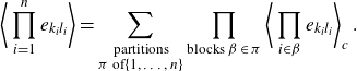 \begin{align}\bigg\langle \prod_{i=1}^n e_{k_il_i}\bigg\rangle=\sum_{\substack{\text{partitions} \\ \text{$\pi$ of$\{1,\dots, n\}$}}} \prod_{\text{blocks $\beta \in \pi$}}\bigg\langle \prod_{i\in \beta} e_{k_i l_i} \bigg\rangle_c\;.\end{align}
There is a similar formula expressing the cumulants in terms of moments [Reference Speed30, equation (1.2)], related to (A1) via Möbius inversion on the partially ordered set of (partitions of) subsets of indices (the partition lattice of
 $[N]\times [N]$
)
$[N]\times [N]$
)
 \begin{equation*}I\,:\!=\,\{k_1l_1,\dots,k_nl_n\}\subset [N]\times [N]\:,\end{equation*}
with
 $|I|=n$
and
$|I|=n$
and
 $[N]\,:\!=\,\{1,\dots,N\}$
. For a quartic potential (2.2), moments and cumulants are only non-zero if n is even and every block
$[N]\,:\!=\,\{1,\dots,N\}$
. For a quartic potential (2.2), moments and cumulants are only non-zero if n is even and every block
 $\beta$
is of even length. For example,
$\beta$
is of even length. For example,
 \begin{align*}\big\langle e_{k_1l_1}e_{k_2l_2}e_{k_3l_3}e_{k_4l_4}\big\rangle&=\big\langle e_{k_1l_1}e_{k_2l_2}e_{k_3l_3}e_{k_4l_4}\big\rangle_c +\big\langle e_{k_1l_1}e_{k_2l_2}\big\rangle_c \big\langle e_{k_3l_3}e_{k_4l_4}\big\rangle_c\\& \quad +\big\langle e_{k_1l_1}e_{k_3l_3}\big\rangle_c \big\langle e_{k_2l_2}e_{k_4l_4}\big\rangle_c+\big\langle e_{k_1l_1}e_{k_4l_4}\big\rangle_c \big\langle e_{k_2l_2}e_{k_3l_3}\big\rangle_c\;.\end{align*}
Note that in our context the moments
 $\big\langle \prod_{i=1}^ne_{k_il_i}\big\rangle$
are invariant under permutations of
$\big\langle \prod_{i=1}^ne_{k_il_i}\big\rangle$
are invariant under permutations of
 $I\,:\!=\,\{k_1l_1,\dots,k_nl_n\}$
so that they only depend on the subset
$I\,:\!=\,\{k_1l_1,\dots,k_nl_n\}$
so that they only depend on the subset
 $I\subset [N]\times [N]$
, but not on the choice of a labelling
$I\subset [N]\times [N]$
, but not on the choice of a labelling
 $I=\{k_1l_1,\dots,k_nl_n\}\simeq [n]$
. By [Reference Speed30, equation (1.2)] the same is then true for the cumulants, i.e.
$I=\{k_1l_1,\dots,k_nl_n\}\simeq [n]$
. By [Reference Speed30, equation (1.2)] the same is then true for the cumulants, i.e.
 $\big\langle \prod_{i\in \beta} e_{k_i l_i} \big\rangle_c$
only depends on the subset
$\big\langle \prod_{i\in \beta} e_{k_i l_i} \big\rangle_c$
only depends on the subset
 $\{k_il_i|\: i\in \beta\}\subset [N]\times [N]$
.
$\{k_il_i|\: i\in \beta\}\subset [N]\times [N]$
.
We restrict our attention to the case that all
 $k_i$
are pairwise different. Then the structure of the Gaußian measure (2.1) (together with the invariance of a trace under cyclic permutations) implies that the cumulant
$k_i$
are pairwise different. Then the structure of the Gaußian measure (2.1) (together with the invariance of a trace under cyclic permutations) implies that the cumulant
 $\big\langle \prod_{i=1}^n e_{k_il_i}\big\rangle_c$
corresponding to
$\big\langle \prod_{i=1}^n e_{k_il_i}\big\rangle_c$
corresponding to
 $I=\{k_1l_1,\dots,k_nl_n\}$
with
$I=\{k_1l_1,\dots,k_nl_n\}$
with
 $|I|=n>0$
is only non-zero if I has a permutation
$|I|=n>0$
is only non-zero if I has a permutation
 $\sigma$
with
$\sigma$
with
 $pr_2=pr_1\circ \sigma$
. Here
$pr_2=pr_1\circ \sigma$
. Here
 \begin{equation*}pr_i\,:\, [N]\times [N]\supset I \longrightarrow [N]\end{equation*}
is the projection onto the corresponding factor for
 $i=1,2$
. By choosing a labelling
$i=1,2$
. By choosing a labelling
 \begin{equation*}I\,:\!=\,\{k_1l_1,\dots,k_nl_n\}\simeq [n]\end{equation*}
as before, this corresponds to a permutation
 $\sigma$
in the symmetric group
$\sigma$
in the symmetric group
 $ \mathcal{S}_n$
, with
$ \mathcal{S}_n$
, with
 $(l_1,\dots,l_n)=\big(k_{\sigma(1)},\dots,k_{\sigma(n)}\big)$
.
$(l_1,\dots,l_n)=\big(k_{\sigma(1)},\dots,k_{\sigma(n)}\big)$
.
Therefore, the cumulant
 $\big\langle \prod_{i=1}^n e_{k_il_i}\big\rangle_c$
only depends on I and the conjugacy class of a permutation in
$\big\langle \prod_{i=1}^n e_{k_il_i}\big\rangle_c$
only depends on I and the conjugacy class of a permutation in
 $\mathcal{S}_n$
(corresponding to the permutation
$\mathcal{S}_n$
(corresponding to the permutation
 $\sigma$
of I with
$\sigma$
of I with
 $pr_2=pr_1\circ \sigma$
), which is again independent of the choice of the labelling of I. In fact such conjugacy classes in
$pr_2=pr_1\circ \sigma$
), which is again independent of the choice of the labelling of I. In fact such conjugacy classes in
 $\mathcal{S}_n$
just correspond to the different cycle types of a permutation in the symmetric group
$\mathcal{S}_n$
just correspond to the different cycle types of a permutation in the symmetric group
 $ \mathcal{S}_n$
. The cycle type of
$ \mathcal{S}_n$
. The cycle type of
 $\sigma$
is the n-tuple
$\sigma$
is the n-tuple
 $(\ell_1(\sigma),\ell_2(\sigma),\dots,\ell_n(\sigma))$
where
$(\ell_1(\sigma),\ell_2(\sigma),\dots,\ell_n(\sigma))$
where
 $\ell_k(\sigma)$
is the number of cycles of length k in
$\ell_k(\sigma)$
is the number of cycles of length k in
 $\sigma$
, with
$\sigma$
, with
 $\sum_{i=1}^n i\ell_i(\sigma)=n$
. The number of cycles in a permutation
$\sum_{i=1}^n i\ell_i(\sigma)=n$
. The number of cycles in a permutation
 $\sigma$
is
$\sigma$
is
 $b(\sigma)=\sum_{i=1}^n \ell_i(\sigma)$
. The number of different cycle types is the partition number p(n), and there are
$b(\sigma)=\sum_{i=1}^n \ell_i(\sigma)$
. The number of different cycle types is the partition number p(n), and there are
 ${n!}/{1^{\ell_1} \ell_1! 2^{\ell_2}\ell_2!\dots n^{\ell_n} \ell_n!}$
permutations with the same cycle type
${n!}/{1^{\ell_1} \ell_1! 2^{\ell_2}\ell_2!\dots n^{\ell_n} \ell_n!}$
permutations with the same cycle type
 $(\ell_1,\dots,\ell_n)$
.
$(\ell_1,\dots,\ell_n)$
.
Conversely, the l-indices of a non-vanishing cumulant
 $\big\langle e_{k_1l_1}\ldots e_{k_nl_n}\big\rangle_c$
are completely determined by the cycle type and the information which k’s belong in which cyclic order to the same cycle. If, after renaming the k’s,
$\big\langle e_{k_1l_1}\ldots e_{k_nl_n}\big\rangle_c$
are completely determined by the cycle type and the information which k’s belong in which cyclic order to the same cycle. If, after renaming the k’s,
 $\big(k_1^1,\dots,k^1_{n_1}\big)$
belong to one cycle,
$\big(k_1^1,\dots,k^1_{n_1}\big)$
belong to one cycle,
 $\big(k_1^2,\dots,k^2_{n_2}\big)$
belong to another cycle, and so on up to the
$\big(k_1^2,\dots,k^2_{n_2}\big)$
belong to another cycle, and so on up to the
 $b^{\text{th}}$
cycle, this information uniquely encodes a cumulant (with
$b^{\text{th}}$
cycle, this information uniquely encodes a cumulant (with
 $n=n_1+\dots+n_b$
)
$n=n_1+\dots+n_b$
)
 \begin{align}N^n \Big\langle \Big(e_{k_1^1k_2^1}e_{k_2^1k_3^1} \ldots e_{k_{n_1}^1k_1^1}\Big) \ldots\Big(e_{k_1^bk_2^b} e_{k_2^bk_3^b} \ldots e_{k_{n_b}^bk_1^b}\Big) \Big\rangle_c\,=\!:\,N^{2-b} G_{\big|k_1^1\dots k_{n_1}^1\big|\dots\big|k_1^b\dots k_{n_b}^b\big|} \;.\end{align}
The power series expansion of the Fourier transform
 $\mathcal{Z}(M)$
into moments (2.3) can be compared with the insertion of (A2) into (A1). The first terms are:
$\mathcal{Z}(M)$
into moments (2.3) can be compared with the insertion of (A2) into (A1). The first terms are:
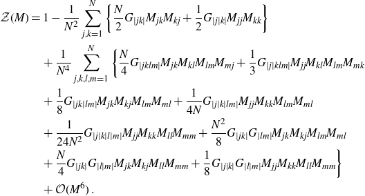 \begin{align}\mathcal{Z}(M)&=1- \frac{1}{N^2} \sum_{j,k=1}^N \bigg\{\frac{N}{2}G_{|jk|} M_{jk}M_{kj}+ \frac{1}{2} G_{|j|k|} M_{jj}M_{kk}\bigg\}\nonumber\\& \quad + \frac{1}{N^4}\sum_{j,k,l,m=1}^N \bigg\{\frac{N}{4}G_{|jklm|} M_{jk} M_{kl}M_{lm}M_{mj}+ \frac{1}{3} G_{|j|klm|} M_{jj}M_{kl} M_{lm}M_{mk}\nonumber\\& \quad + \frac{1}{8} G_{|jk|lm|} M_{jk}M_{kj}M_{lm}M_{ml}+ \frac{1}{4N}G_{|j|k|lm|} M_{jj}M_{kk} M_{lm}M_{ml}\nonumber\\& \quad + \frac{1}{24N^2} G_{|j|k|l|m|} M_{jj}M_{kk}M_{ll}M_{mm}+ \frac{N^2}{8} G_{|jk|} G_{|lm|} M_{jk}M_{kj} M_{lm}M_{ml}\nonumber\\& \quad + \frac{N}{4} G_{|jk|} G_{|l|m|} M_{jk}M_{kj} M_{ll}M_{mm}+ \frac{1}{8} G_{|j|k|} G_{|l|m|}M_{jj} M_{kk}M_{ll} M_{mm}\bigg\}\nonumber\\& \quad + \mathcal{O}(M^6)\;.\end{align}
Appendix B. Equations for the second cumulant
We derive here equations for the two non-vanishing second-order cumulants
 $G_{|ab|} =\frac{1}{N}\langle e_{ab} e_{ba}\rangle_c$
of cycle type (0, 1) (i.e. one cycle ab of length 2) and
$G_{|ab|} =\frac{1}{N}\langle e_{ab} e_{ba}\rangle_c$
of cycle type (0, 1) (i.e. one cycle ab of length 2) and
 $G_{|a|b|}=\langle e_{aa} e_{bb}\rangle_c$
of cycle type (2, 0) (i.e. two cycles a and b of length 1). To distinguish
$G_{|a|b|}=\langle e_{aa} e_{bb}\rangle_c$
of cycle type (2, 0) (i.e. two cycles a and b of length 1). To distinguish
 $G_{|ab|}$
and
$G_{|ab|}$
and
 $G_{|a|b|}$
we require
$G_{|a|b|}$
we require
 $a\neq b$
.
$a\neq b$
.
We start from (2.7) with
 $\mathcal{Z}(M)$
given by (A3), apply
$\mathcal{Z}(M)$
given by (A3), apply
 $({N(E_a+E_b)}/{\textrm{i}}) ({\partial}/{\partial M_{ba}})$
and put
$({N(E_a+E_b)}/{\textrm{i}}) ({\partial}/{\partial M_{ba}})$
and put
 $M=0$
. For
$M=0$
. For
 $a\neq b$
this gives the following result (the underlining should be ignored for the moment; we explain it later):
$a\neq b$
this gives the following result (the underlining should be ignored for the moment; we explain it later):
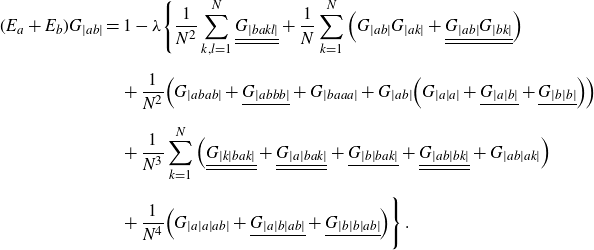 \begin{align}(E_a+E_b)G_{|ab|}&=1-\lambda\Bigg\{\frac{1}{N^2}\sum_{k,l=1}^{N} \underline{\underline{G_{|bakl|}}}+ \frac{1}{N}\sum_{k=1}^{N} \Big(G_{|ab|}G_{|ak|}+\underline{\underline{G_{|ab|}G_{|bk|}}}\Big)\nonumber\\[6pt]& \quad +\frac{1}{N^2}\Big(G_{|abab|}+\underline{G_{|abbb|}} +G_{|baaa|}+G_{|ab|}\Big(G_{|a|a|}+\underline{G_{|a|b|}}+\underline{G_{|b|b|}}\Big)\Big)\nonumber\\[6pt]& \quad +\frac{1}{N^3} \sum_{k=1}^{N} \Big(\underline{\underline{G_{|k|bak|}}}+\underline{\underline{G_{|a|bak|}}}+ \underline{G_{|b|bak|}}+\underline{\underline{G_{|ab|bk|}}}+G_{|ab|ak|}\Big)\nonumber\\[6pt]& \quad +\frac{1}{N^4} \Big(G_{|a|a|ab|}+\underline{G_{|a|b|ab|}}+\underline{G_{|b|b|ab|}}\Big)\Bigg\}\;.\end{align}
Next, we set
 $b \equiv a$
in (2.7) for
$b \equiv a$
in (2.7) for
 $\mathcal{Z}(M)$
given by (A3), apply
$\mathcal{Z}(M)$
given by (A3), apply
 $({N^2(E_a+E_a)}/{\textrm{i}}) ({\partial}/{\partial M_{bb}})$
for
$({N^2(E_a+E_a)}/{\textrm{i}}) ({\partial}/{\partial M_{bb}})$
for
 $a \neq b$
and obtain for
$a \neq b$
and obtain for
 $M=0$
(ignore again the underlining):
$M=0$
(ignore again the underlining):
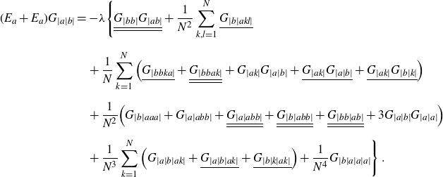 \begin{align}(E_a+E_a)G_{|a|b|}&=-\lambda\Bigg\{\underline{\underline{G_{|bb|}G_{|ab|}}}+\frac{1}{N^2}\sum_{k,l=1}^{N} \underline{G_{|b|akl|}}\nonumber\\[6pt]& \quad +\frac{1}{N}\sum_{k=1}^{N} \Big(\underline{G_{|bbka|}}+\underline{\underline{G_{|bbak|}}}+G_{|ak|}G_{|a|b|}+\underline{G_{|ak|}G_{|a|b|}}+\underline{G_{|ak|}G_{|b|k|}}\Big)\nonumber\\[6pt]& \quad +\frac{1}{N^2}\Big(G_{|b|aaa|}+G_{|a|abb|}+\underline{\underline{G_{|a|abb|}}}+\underline{\underline{G_{|b|abb|}}}+\underline{\underline{G_{|bb|ab|}}}+3 G_{|a|b|}G_{|a|a|}\Big)\nonumber\\[6pt]& \quad +\frac{1}{N^3}\sum_{k=1}^{N} \Big(G_{|a|b|ak|}+\underline{G_{|a|b|ak|}}+\underline{G_{|b|k|ak|}}\Big)+\frac{1}{N^4} G_{|b|a|a|a|}\Bigg\}\;.\end{align}
Equations (B1) and (B2) are the analogues of Dyson–Schwinger equations in quantum field theory. In this form they provide little information because the right-hand sides are too complicated. We will now establish from the equations of motion (2.7) two other identities which collect the underlined terms in (B1) and (B2) into a function of the left-hand sides.
To establish the identities, set
 $b\mapsto k$
in (2.7) and apply
$b\mapsto k$
in (2.7) and apply
 $({N(E_a+E_k)}/{\textrm{i}}) ({\partial}/{\partial M_{kb}})$
. Next, set
$({N(E_a+E_k)}/{\textrm{i}}) ({\partial}/{\partial M_{kb}})$
. Next, set
 $a\mapsto k$
in (2.7) and apply
$a\mapsto k$
in (2.7) and apply
 $({N(E_b+E_k)}/{\textrm{i}}) ({\partial}/{\partial M_{ak}})$
. Take the difference of both equations and sum over k:
$({N(E_b+E_k)}/{\textrm{i}}) ({\partial}/{\partial M_{ak}})$
. Take the difference of both equations and sum over k:
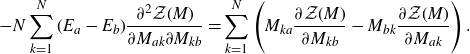 \begin{align}-N\sum_{k=1}^{N}(E_a-E_b)\frac{\partial^2\mathcal{Z}(M)}{\partial M_{ak} \partial M_{kb}}= \sum_{k=1}^{N}\Bigg(M_{ka} \frac{\partial\mathcal{Z}(M)}{\partial M_{kb}}-M_{bk} \frac{\partial\mathcal{Z}(M)}{\partial M_{ak}}\Bigg)\;.\end{align}
This is a Ward–Takahashi identity first discovered in [Reference Disertori, Gurau, Magnen and Rivasseau9]. The strategy which we follow here was suggested in [Reference Grosse and Wulkenhaar17]. We insert (A3) into (B3) and evaluate the derivatives for
 $a\neq b$
:
$a\neq b$
:
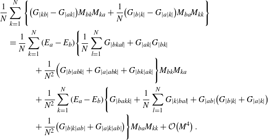 \begin{align}&\frac{1}{N}\sum_{k=1}^{N}\Bigg\{\big(G_{|kb|} - G_{|ak|}\big) M_{bk} M_{ka}+ \frac{1}{N}\big(G_{|b|k|} -G_{|a|k|}\big) M_{ba} M_{kk} \Bigg\}\nonumber\\& \quad =\frac{1}{N}\sum_{k=1}^{N} (E_a-E_b)\Bigg\{ \frac{1}{N} \sum_{l=1}^{N} G_{|bkal|}+G_{|ak|} G_{|bk|}\nonumber\\[-0.5ex]&\qquad \qquad +\frac{1}{N^2} \Big(G_{|b|abk|} +G_{|a|abk|} + G_{|bk|ak|}\Bigg\}M_{bk} M_{ka}\nonumber\\&\qquad \qquad + \frac{1}{N^2}\sum_{k=1}^{N} (E_a-E_b)\Bigg\{G_{|bakk|}+ \frac{1}{N}\sum_{l=1}^{N} G_{|k|bal|}+ G_{|ab|} \big(G_{|b|k|}+ G_{|a|k|}\big)\nonumber\\[-0.5ex]&\qquad \qquad + \frac{1}{N^2} \big(G_{|b|k|ab|}+G_{|a|k|ab|}\big)\Bigg\}M_{ba} M_{kk}+\mathcal{O}\big(M^4\big)\;.\end{align}
For the next steps we assume that the functions
 $G_{..k_i..}$
under consideration are evaluations of holomorphic functions in several complex variables at points
$G_{..k_i..}$
under consideration are evaluations of holomorphic functions in several complex variables at points
 $E_{k_i}$
in the holomorphicity domain. See the discussion after (3.1). Applying to (B4) the operators
$E_{k_i}$
in the holomorphicity domain. See the discussion after (3.1). Applying to (B4) the operators
 $N \partial^2/\big(\partial M_{bp} \partial M_{pa}\big)$
or
$N \partial^2/\big(\partial M_{bp} \partial M_{pa}\big)$
or
 $N^2 \partial^2/\big(\partial M_{ba} \partial M_{pp}\big)$
for
$N^2 \partial^2/\big(\partial M_{ba} \partial M_{pp}\big)$
for
 $a\neq p\neq b$
gives two independent equations. Under the holomorphicity assumption they extend continuously to
$a\neq p\neq b$
gives two independent equations. Under the holomorphicity assumption they extend continuously to
 $p=a$
and
$p=a$
and
 $p=b$
. After exchanging
$p=b$
. After exchanging
 $p\leftrightarrow b$
, these equations read
$p\leftrightarrow b$
, these equations read
 \begin{align}-\frac{G_{|pb|} - G_{|ab|}}{E_p-E_a}&=\frac{1}{N} \sum_{k=1}^{N} G_{|bakp|}+G_{|ab|} G_{|bp|}+\frac{1}{N^2} \big(G_{|p|bap|} +G_{|a|bap|} + G_{|bp|ab|}\big) \;,\end{align}
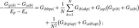 \begin{align}-\frac{G_{|p|b|} - G_{|a|b|}}{E_p-E_a}&=G_{|bbpa|}+ \frac{1}{N}\sum_{k=1}^{N} G_{|b|akp|}+ G_{|ap|} \big(G_{|p|b|}+ G_{|a|b|}\big)\nonumber\\&\qquad + \frac{1}{N^2} \big(G_{|b|p|ap|}+G_{|a|b|ap|}\big)\;;\end{align}
they hold for
 $p\neq a$
. By the holomorphicity assumption the equations (B5) and (B6) extend continuously to
$p\neq a$
. By the holomorphicity assumption the equations (B5) and (B6) extend continuously to
 $p=a$
. Then, summing (B5) over p collects the double-underlined terms in (B1) into
$p=a$
. Then, summing (B5) over p collects the double-underlined terms in (B1) into
 $- ({1}/{N})\sum_{p=1}^{N}\! {\big(G_{|pb|} - G_{|ab|}\big)}\big/{\big(E_p-E_a\big)}$
, and the case
$- ({1}/{N})\sum_{p=1}^{N}\! {\big(G_{|pb|} - G_{|ab|}\big)}\big/{\big(E_p-E_a\big)}$
, and the case
 $p=b$
of (B6) collects the single-underlined terms in (B1). Similarly, summing (B6) over p collects the single-underlined terms in (B2) into
$p=b$
of (B6) collects the single-underlined terms in (B1). Similarly, summing (B6) over p collects the single-underlined terms in (B2) into
 $-\frac{1}{N}\sum_{p=1}^{N}{\big(G_{|p|b|} - G_{|a|b|}\big)}\big/{\big(E_p-E_a\big)}$
, and the case
$-\frac{1}{N}\sum_{p=1}^{N}{\big(G_{|p|b|} - G_{|a|b|}\big)}\big/{\big(E_p-E_a\big)}$
, and the case
 $p=b$
of (B5) collects the double-underlined terms in (B2):
$p=b$
of (B5) collects the double-underlined terms in (B2):
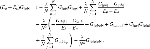 \begin{align}(E_a+E_b)G_{|ab|}&=1-\frac{\lambda}{N}\sum_{p=1}^{N} G_{|ab|}G_{|ap|}+\frac{\lambda}{N}\sum_{p=1}^{N}\frac{G_{|pb|}-G_{|ab|}}{E_p-E_a}\nonumber\\& \quad -\frac{\lambda}{N^2}\Bigg({-}\frac{G_{|b|b|}-G_{|a|b|}}{E_b-E_a}+G_{|abab|} +G_{|baaa|} +G_{|ab|}G_{|a|a|}\nonumber\\&\quad +\frac{1}{N} \sum_{p=1}^{N}G_{|ab|ap|}\Bigg)-\frac{\lambda}{N^4} G_{|a|a|ab|}\;,\end{align}
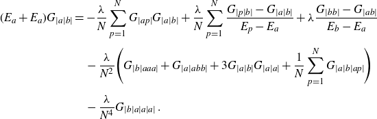 \begin{align}(E_a+E_a)G_{|a|b|}&=-\frac{\lambda}{N}\sum_{p=1}^{N} G_{|ap|}G_{|a|b|}+\frac{\lambda}{N}\sum_{p=1}^{N}\frac{G_{|p|b|}-G_{|a|b|}}{E_p-E_a}+\lambda\frac{G_{|bb|}-G_{|ab|}}{E_b-E_a}\nonumber\\[3pt]&\quad -\frac{\lambda }{N^2}\Bigg(G_{|b|aaa|}+G_{|a|abb|}+3 G_{|a|b|}G_{|a|a|}+\frac{1}{N}\sum_{p=1}^{N} G_{|a|b|ap|}\Bigg)\nonumber\\[3pt]&\quad -\frac{\lambda}{N^4} G_{|b|a|a|a|}\;.\end{align}
These identities have been found in [Reference Grosse and Wulkenhaar17] (by a faster, but less elementary approach).
Identities of such type can be solved by a further expansion of all arising functions
 $G_{\dots}$
as formal power series in
$G_{\dots}$
as formal power series in
 $N^{-2}$
,
$N^{-2}$
,
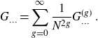 \begin{align}G_{\dots}=\sum_{g=0}^\infty \frac{1}{N^{2g}} G^{(g)}_{\dots}\;.\end{align}
With the convention that
 $({1}/{N})\sum_1^{N}$
is of order
$({1}/{N})\sum_1^{N}$
is of order
 $N^0$
, the coefficient of
$N^0$
, the coefficient of
 $N^{-2g}$
in (B7) reads
$N^{-2g}$
in (B7) reads
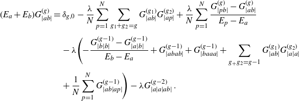 \begin{align}(E_a+E_b)G_{|ab|}^{(g)}&=\delta_{g,0}-\frac{\lambda}{N}\sum_{p=1}^{N} \sum_{g_1+g_2=g} G_{|ab|}^{(g_1)}G_{|ap|}^{(g_2)}+\frac{\lambda}{N}\sum_{p=1}^{N}\frac{G_{|pb|}^{(g)}-G_{|ab|}^{(g)}}{E_p-E_a}\nonumber\\[3pt]& \quad -\lambda\Bigg({-}\frac{G_{|b|b|}^{(g-1)}-G_{|a|b|}^{(g-1)}}{E_b-E_a}+G_{|abab|}^{(g-1)} +G_{|baaa|}^{(g-1)}+\sum_{g_+g_2=g-1} G_{|ab|}^{(g_1)}G_{|a|a|}^{(g_2)}\nonumber\\[3pt]&\quad +\frac{1}{N} \sum_{p=1}^{N}G_{|ab|ap|}^{(g-1)}\Bigg)-\lambda G_{|a|a|ab|}^{(g-2)}\;.\end{align}
For the degree or genus
 $g=0$
we thus obtain the closed equation (3.1) for
$g=0$
we thus obtain the closed equation (3.1) for
 $G_{|ab|}^ {(0)}$
. Similarly, the restriction of (B8) to the degree or genus
$G_{|ab|}^ {(0)}$
. Similarly, the restriction of (B8) to the degree or genus
 $g=0$
is (6.1). Both equations have been solved in this paper.
$g=0$
is (6.1). Both equations have been solved in this paper.
Acknowledgements
Our work was supportedFootnote 4 by the Cluster of Excellence Mathematics Münster. RW would like to thank Harald Grosse and Alexander Hock for the collaboration which provided the basis for this paper.


 Open access