2. Cyclic Proof Systems

We begin by giving a general account of cyclic proof systems and their associated notion of cyclic proof. We illustrate the definitions by presenting a cyclic proof system for the modal $\mu$ -calculus from the literature.

A tree is a finite, non-empty set of sequences $T\subseteq \omega^*$ which is prefix closed, that is, if $tn \in T$ for $t \in \omega^*$ and $n \in \omega$ then $t \in T$ as well. We call $t \in T$ a node of T and any $tn \in T$ a child of t. A node $t\in T$ is a leaf of T if it has no children. The root of any tree T thus is the empty sequence $\varepsilon \in \omega^*$ . A cyclic tree is a pair $C = (T, \beta)$ consisting of a tree T and a partial function $\beta \colon \mathrm{Leaf}(T) \to T$ mapping (some) leaves of T to nodes of T with $\beta(s) \not\in \mathrm{dom}(\beta)$ for all $s \in \mathrm{dom}(\beta)$ . Each $s \in\mathrm{dom}(\beta)$ is called a bud and $\beta(s)$ its companion.

A derivation system is a triple consisting of a set of sequents , a set $\mathcal{R}$ of derivation rules and a rule interpretation such that for each $r \in \mathcal{R}$ , for some $n \in \omega$ . In this case, we call $\Gamma$ the conclusion of r and the $\Delta_i$ its premises. Henceforth, we refer to a derivation system simply by $\mathcal{R}$ . An $\mathcal{R}$ -pre-proof is a triple $\Pi = (C, \lambda, \delta)$ consisting of a cyclic tree $C = (T, \beta)$ together with a labelling such that $\lambda(t) = \lambda(\beta(t))$ for every $t \in \mathrm{dom}(\beta)$ . $\delta : T \setminus \mathrm{dom}(\beta) \to \mathcal{R}$ is a function with $\rho(\delta(t)) = (\Gamma,\Delta_1, \ldots, \Delta_n)$ , $\lambda(t) = \Gamma$ and $\lambda(ti)=\Delta_i$ where $\mathrm{Chld}(t) =\{t1, \ldots, tn\}$ for each $t \in \mathrm{dom}(\delta)$ . The sequent $\lambda(\varepsilon)$ is called the endsequent of $\Pi$ .

We denote by the set of $\mathcal{R}$ -pre-proofs. A cyclic proof system is a tuple consisting of a derivation system and a set called $\mathcal{R}$ -proofs. A pre-proof is said to satisfy the soundness condition of $\mathcal{R}$ if is an $\mathcal{R}$ -proof. An $\mathcal{R}$ -proof with endsequent $\Gamma$ is called a proof of $\Gamma$ . We extend the naming convention for derivation systems to cyclic derivation systems, referring to by $\mathcal{R}$ .

To illustrate these notions, we present a cyclic proof system for the modal $\mu$ -calculus. It will also serve as an example motivating the abstract definitions of Sections 3 and 4. This presentation of the system is taken from Afshari and Leigh (Reference Afshari and Leigh2017) and is an adaptation of the tableaux of Niwiński and Walukiewicz (Reference Niwiński and Walukiewicz1996). The choice of logic for this example is secondary, the main focus being the cyclic aspects of the proof system.

For a set of propositional letters and a countable set of variables, the $\mu$ -formulas are given by the following grammar:

If occur in $\varphi$ , we say x subsumes y, writing $x <_\varphi y$ , if $\sigma y.\psi$ occurs as a subformula of $\varphi$ for some $\sigma \in \{\mu, \nu\}$ and $\psi$ , and furthermore x is free in $\sigma y.\psi$ . If the relation $<_\varphi$ is a strict preorder, we call $\varphi$ well-named. In the remainder of this article, we assume all $\mu$ -formulas are well-named. This is a reasonable restriction as any $\mu$ -formula is $\alpha$ -equivalent to a well-named one. Any $\mu$ -formula is positive in all variables. The fixed-point formulas $\mu x.\varphi$ and $\nu x.\varphi$ denote, respectively, the least and greatest fixed point of the semantic counterpart to the function $x\mapsto\varphi(x)$ . These are well defined by the observation on positivity and the Knaster–Tarski theorem. The semantics of the modalities and connectives are as in the modal logic K.

The derivation rules of the cyclic $\mu$ -calculus are given in Fig. 1. The sequents of this calculus are finite sets of $\mu$ -formulas. Not all pre-proofs derive valid endsequents. For example, $\mu x.\Box x$ is invalid but is concluded by the $\mu$ -pre-proof given in Fig. 2. It is thus necessary to impose an additional soundness condition which delineates $\mu$ -proofs from $\mu$ -pre-proofs.

Figure 1. Derivation rules of the modal $\mu$ -calculus. $\Gamma$ ranges over finite sets of formulas; $\varphi[\psi / x]$ denotes the standard substitution of $\psi$ for x in $\varphi$ .

Figure 2. A $\mu$ -pre-proof of an invalid $\mu$ -formula. The dashed arrow represents the bud-companion relation $\beta$ .

A branch through a pre-proof $((T, \beta), \lambda, \delta)$ is an infinite sequence $t \in T^\omega$ such that $t_0 = \varepsilon$ and for any $t_i$ , either (a) $t_{i + 1} \in \mathrm{Chld}(t_i)$ or (b) $t_i \in \mathrm{dom}(\beta)$ and $t_{i + 1} = \beta(t_i)$ . This induces the sequence with $\Gamma_i := \lambda(t_i)$ and the partially defined $r : \omega \to \mathcal{R}$ with $r_i:= \delta(t_i)$ , both of which we use interchangeably with $t \in T^\omega$ to denote a branch.

Given a branch $(\Gamma_i)_{i \in \omega}$ through a $\mu$ -pre-proof, a formula $\varphi' \in \Gamma_{i + 1}$ is called a precursor of $\varphi \in \Gamma_i$ , written $\varphi' \leftarrow_i\varphi$ , if $t_{i + 1} \in \mathrm{Chld}(t_i)$ and either $\varphi$ is principal in $r_i$ , that is, $\varphi$ is ‘altered by $r_i$ ’, and $\varphi'$ is one of the residual formulas, or $\varphi$ is not principal in $r_i$ and $\varphi = \varphi'$ . If $t_i \in \mathrm{dom}(\beta)$ and $\varphi = \varphi'$ then $\varphi' \leftarrow_i \varphi$ as well. A sequence of formulas $(\varphi_i)_{i \in \omega}$ is called a trace along $(\Gamma_i)_{i \in \omega}$ if $\varphi_{i + 1} \leftarrow_i \varphi_{i}$ for all $i \in \omega$ . It is easily observed that the subsumption order is preserved along traces, that is, $\mathord{<_{\varphi_{i + 1}}} \subseteq \mathord{<_{\varphi_i}}$ whenever $\varphi_{i + 1} \leftarrow_i \varphi_i$ , which is why we henceforth associate with each trace $(\varphi_i)_{i \in \omega}$ a global subsumption order $\mathord{<_\varphi} := \mathord{<_{\varphi_0}} = \bigcup_{i \in \omega} \mathord{<_{\varphi_i}}$ .

Let $(\Gamma_i)_{i \in \omega}$ be a branch through a $\mu$ -pre-proof and $(\varphi_i)_{i \in \omega}$ a trace along it. The trace is called a $\nu$ -trace if there exists an such that $\varphi_i = \nu x.\psi$ and $\varphi_{i + 1} = \psi[\varphi_i / x]$ for infinitely many $i \in \omega$ , and furthermore for any if there are infinitely many $\varphi_i = \mu y.\theta$ then $x <_{\varphi} y$ . In other words, there is a greatest fixed-point variable x that occurs infinitely often and subsumes all infinitely occurring $\mu$ -variables. A $\mu$ -proof is a $\mu$ -pre-proof that satisfies the global trace condition, that is, every infinite branch has a $\nu$ -trace. As the unique branch through the pre-proof in the example of Fig. 2 does not have a $\nu$ -trace, it fails to be a proof.

At this point, we want to clearly distinguish between a ‘trace condition’ and a ‘global trace condition’. A trace condition is a specification of which traces along infinite branches of a pre-proof are considered progressing. A global trace condition is a certain type of condition on cyclic proofs, usually formulated via a trace condition, used to ensure soundness of proofs. Alternative soundness conditions have been considered, such as the reset condition (Jungteerapanich Reference Jungteerapanich, Giese and Waaler2009), induction orders (Sprenger and Dam Reference Sprenger and Dam2003) and trace manifolds (Brotherston Reference Brotherston2006). These soundness conditions are often still defined in reference to a trace condition, or at least its implicit notion of progress. It is, therefore, possible for two differently formulated soundness conditions for a certain derivation system to share the same underlying trace condition. For example, this is the case for the GTC of the $\mu$ -proofs specified above and the reset proof system for the modal $\mu$ -calculus given by Stirling (Reference Stirling2013).

3. Abstracting the Trace Condition

In this section, we demonstrate our formalism for capturing the trace conditions of cyclic proof systems. It encompasses two levels of abstraction: The notion of a trace category which captures what it means to be a trace condition, and a family of concrete trace categories, generated by the notion of an activation algebra.

An abstract notion of trace condition requires an abstract notion of branches through a proof. Working in a category theoretical framework, we observe that branches are infinite sequences of rule applications and identify them with infinite sequences of morphisms called paths. A trace condition is then a condition on such paths which is invariant under certain path transformations.

A semi-category is a category which may not have (all) identity morphisms. That is, a semi-category $\mathcal{C}$ consists of a collection of objects $\mathrm{Ob}(\mathcal{C})$ and collections of morphisms between each pair of objects $X, Y \in\mathrm{Ob}(\mathcal{C})$ . There is a composition which is associative. A semi-functor is a semi-category homomorphism. That is, for semi-categories $\mathcal{C}, \mathcal{D}$ , a semi-functor $F : \mathcal{C} \to \mathcal{D}$ consists of a map on objects $F_0 : \mathrm{Ob}(\mathcal{C}) \to \mathrm{Ob}(\mathcal{D})$ and a further map $F_2$ on morphisms of C such that for $f : X \to Y$ we have $F_1(f) : F_0(X)\to F_0(Y)$ . $F_1$ distributes over the composition operation, that is, $F_1(g \circ f) = F_1(g) \circ F_1(f)$ . As is also common for standard functors, we denote both $F_0$ and $F_1$ by F.

The standard $<$ -ordering of the natural numbers $\omega$ induces a semi-category whose objects are the natural numbers and in which there is a (unique) morphism between n and m, denoted ‘ $n < m : n \to m$ ’, if $n < m$ . The $\leq$ -ordering induces an analogous proper category. In this article, we denote both of these categories by $\omega$ ; which one is meant will be clear from the context.

A path through a category $\mathcal{T}$ is a functor $P \colon \omega \to \mathcal{T}$ . Given $P, P' \colon \omega \to \mathcal{T}$ , we call P a subpath of P’, written $P \subseteq P'$ , if there is a semi-functor $S \colon \omega \to \omega$ between the $\omega$ -semi-categories such that $P = P' \circ S$ . The transitive, symmetric closure of $\subseteq$ is denoted $\sim$ . This means $P \subseteq P'$ holds if P’ can be transformed into the P by applying a combination of two path transformations: (1) discarding a finite prefix of path P’, for example, by taking $S(m) := m + n$ . (2) Composing morphisms along P’. For example, if P’ is of the form

$$X_0^0 \xrightarrow{R^0_0} X_0^1 \xrightarrow{R^1_0} \cdots X_0^{n_0} \xrightarrow{R_0^{n_0}} X_1^0 \xrightarrow{R_1^0} \cdots X_1^{n_1} \xrightarrow{R_1^{n_1}} X_2^0 \xrightarrow{R_2^0} \cdots X_2^{n_2} \xrightarrow{R_2^{n_2}} ...$$

then $P \subseteq P'$ for the path P below

$$X_0^0 \xrightarrow{R^{n_0}_0 \circ \cdots \circ R^0_0} X_1^0 \xrightarrow{R^{n_1}_1 \circ \cdots \circ R^{0}_1 } X_2^0 \xrightarrow {R^{n_2}_2 \circ \cdots \circ R^{0}_2 } ...$$

witnessed by $S(i) := \sum_{j < i} (n_j + 1)$ .

Note that the notion of trace category in the above definition is unrelated to the ‘traced monoidal categories’ of Joyal et al. (Reference Joyal, Street and Verity1996).

Definition 3.3. Let $\mathcal{A}$ be an activation algebra. The $\mathcal{A}$ -activated trace category $\mathcal{T}_\mathcal{A}$ has as its objects the finite sets. The morphisms between sets X, Y are relations $R \subseteq X \times \mathcal{A} \times Y$ . The identities are $1_X := \{(x, 0, x) ~|~ x \in X\}$ . We often write $x R^a y$ to mean $(x, a, y) \in R$ . Given morphisms $R \colon X \to Y, R' \colon Y \to Z$ , their composition is specified by $(x, c, z) \in R' \circ R$ iff

$$\exists y \in Y \exists a, b \in A.\;(x, a, y) \in R \mathrm{ and } (y, b, z) \in R' \mathrm{ and } a \vee b = c.$$

A path $P \colon \omega \to \mathcal{T}_\mathcal{A}$ satisfies the trace condition if there exists a subpath $P' \subseteq P$ and a sequence $\sigma \colon \Pi i \in \omega. P'(i)$ along it such that $\sigma_i P'(i < i + 1)^\alpha \sigma_{i + 1}$ for all $i \in \omega$ .

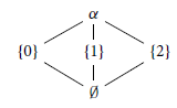
Example 3.3. More complex examples are the ‘k out of n’ algebras for $0 < k \leq n$ given by ${n \choose k} := (A, \leq, \vee, \emptyset, \alpha)$ where $A := \{X \subseteq n ~|~ \left|X\right| < k\} \cup \{\alpha\}$ , the order $\leq$ is such that $X \leq Y$ iff $X \subseteq Y$ for $X, Y \subseteq n$ , and $a \leq \alpha$ for all $a \in A$ . More concretely, observe the Hasse diagram of ${3 \choose 2}$ .

The idea behind ${n \choose k}$ is to view the singleton sets $\{i\}$ as ‘events’ which can occur along a trace. To achieve activation, k distinct ‘events’ need to take place along a segment. As opposed to $\mathbb{B}$ and $\mathbb{F}$ , we are not yet aware of a cyclic proof system whose trace condition is best expressed in terms of some ${n \choose k}$ (except of course ${1 \choose 1}$ which the same as $\mathbb{B}$ ). We conjecture that cyclic proof systems whose trace condition is naturally modelled in some non-trivial ${n \choose k}$ would require a kind of fairness condition of their progressing traces.

For the converse direction, let $P = Q \circ S$ and suppose Q satisfies the trace condition as witnessed by $Q' = Q \circ S'$ and a sequence $\sigma \colon \Pi i \in \omega. Q'(i)$ . It remains to show that there is $P' \subseteq P$ and a suitable sequence $\sigma'' : \Pi i \in \omega.P'(i)$ along it. By fixing $b := S'(0)$ and analysing Definition 3.3, one can conclude there are two sequences $\sigma' \colon \Pi i \in \omega. Q(b + i)$ and $a \colon \omega \to \mathcal{A}$ such that $\sigma'_i\, Q(b + i < b + i + 1)^{a_i}\,\sigma'_{i + 1}$ with $a_i \leq \alpha$ . For $i_j := S'(j) - b$ , we then have $\sigma'_{i_j} = \sigma_j$ and $\bigvee_{i = i_j}^{i < i_{j + 1}} a_i = \alpha$ . Now construct the following sequence:

\begin{align*} k_0 & \,:= \mathrm{least } i \in \omega \mathrm{ such that } S(i) \geq b \\ k_{n + 1} & \,:= \mathrm{least } i > k_n \mathrm{ s.t. } S(k_n) \leq S'(j) < S'(j + 1) \leq S(i) \mathrm{ for some } j \in \omega \end{align*}

We claim setting $S''(i) := S(k_i)$ induces the desired subpath $P' := Q \circ S'' P$ with $P'(i) = P(k_i)$ as witnessed by $\sigma'' \colon \Pi i \in \omega. P'(i)$ given by $\sigma''_{i} := \sigma'_{S(k_i)}$ . For this, we need to check that $\sigma''_{i + 1}\,P'(i < i + 1)^\alpha\,\sigma''_{i + 1}$ . Let $j \in \omega$ be such that $S''(i) \leq S'(j) < S'(j + 1) \leq S''(i + 1)$ . Then, $P'(i < i + 1) = Q(b + i_{j + 1} \leq S(k_{i + 1})) \circ Q(b + i_j < b + i_{j + 1}) \circ Q(S(k_i) \leq b + i_j)$ , meaning

$$\left(\sigma''_i, \underbrace{\bigvee_{l = b + i_{j + 1}}^{l < S(k_{i + 1})} a_{l - b}}_{\leq \alpha} \vee \underbrace{\bigvee_{l = i_j}^{l < i_{j + 1}} a_l}_{= \alpha} \vee \underbrace{\bigvee_{l = S(k_i)}^{l < b + i_{j}} a_{l - b}}_{\leq \alpha}, \underbrace{\sigma'_{k_{i + 1} - b}}_{= \sigma''_{i + 1}}\right) \in P'(i < i + 1)$$

and thus $(\sigma''_i, \alpha, \sigma''_{i + 1}) \in P'(i < i + 1)$ as desired.

We now proceed to demonstrate how trace categories can be used to specify the trace conditions and, thereby, the GTCs of cyclic proof systems. Fix a derivation system and a trace category $\mathcal{T}$ . A trace interpretation $\iota : \mathcal{R} \to \mathcal{T}$ consists of a function mapping sequents to their trace sets and for each rule $r\in \mathcal{R}$ with $\rho(r) = (\Gamma, \Delta_1,\ldots, \Delta_n)$ a morphism $r_i : \iota(\Gamma) \to \iota(\Delta_i)$ for each $1 \leq i \leq n$ called a trace map. Let $(C, \lambda, \delta)$ be a pre-proof and $t \in T^\omega$ be a branch through C. Its corresponding path $P : \omega \to \mathcal{T}$ is defined as follows:

$$P(i) := \iota(\lambda(\pi_i)) \qquad P(i < i + 1) := \begin{cases} r_j : \iota(\lambda(\pi_i)) \to \iota(\lambda(\pi_{i + 1})) & \pi_i \not\in \mathrm{Leaf}(T) \mathrm{ and } \pi_{i + 1} = \pi j \\ 1_{P(i)} & \pi_i \in \mathrm{dom}(\beta) \end{cases}$$

This induces a cyclic proof system in which contains those $\mathcal{R}$ -pre-proofs for which every induced path $P : \omega \to \mathcal{T}$ through them satisfies the trace condition of $\mathcal{T}$ .

In the following, we demonstrate how to specify the trace condition for the modal $\mu$ -calculus by a trace interpretation $\iota : \mu \to \mathbb{F}$ .

Definition 3.4. The trace interpretation $\iota \colon \mu \to \mathcal{T}_\mathbb{F}$ is given by in which . For each $r \in \mu$ with $\rho(r) = (\Gamma, \Delta_1, \ldots, \Delta_n)$ , the trace maps $r_i \colon \iota(\Gamma) \to \iota(\Delta)$ are defined by $ r_i := \{((\varphi, x), a^*, (\varphi', x)) ~|~ \varphi' \leftarrow_r^i \varphi \} $ where $a^*$ is defined by:

$$ a^* := \begin{cases} 2, & \mathrm{ if }r \mathrm{ instance of } \mu, \varphi = \mu y.\theta, \varphi' = \theta[\mu y.\theta / y] \mathrm{ and } y <_{\varphi} x, \\ 1, & \mathrm{ if } r \mathrm{ instance of } \nu, \varphi = \nu x.\theta, \varphi' = \theta[\nu x. \theta / x], \\ 0, & \mathrm{ otherwise.} \end{cases} $$

Suppose $(\Gamma_i)_{i \in \omega}$ has a $\nu$ -trace $(\varphi_i)_{i \in \omega}$ . Then there exists bounded by a $\nu$ -quantifier and an increasing sequence $(j_i)_{i \in \omega}$ such that

1. (i) $\varphi_{j_i} = \nu x.\psi$ and $\varphi_{j_i + 1} = \psi[\varphi_{j_i} / x]$ , and

2. (ii) no formula $\mu y.\theta$ with $y <_{\varphi} x$ is unfolded along $(\varphi_{i})_{i>j_0}$ .

The subpath $P \circ S \subseteq P$ induced by $S(i) := j_{i}$ and the sequence $\sigma_i := (\varphi_{j_{i}}, x)$ witness that P satisfies the trace condition: clearly always $(\sigma_i, a, \sigma_{i + 1}) \in P(j_{i}, j_{i + 1})$ for some $a \in \mathbb{F}$ . We know $1 \leq a$ since between $\Gamma_{j_i}$ and $\Gamma_{j_{i + 1}}$ , $\nu x.\psi$ is unfolded, and further $a < 2$ , as no $\mu y.\theta$ with $y <_{\varphi} x$ is unfolded after $j_0$ , yielding $a = 1$ as desired.

Conversely, suppose P satisfied the trace condition. Then there exist $S \colon \omega \to \omega$ and $\sigma \colon \Pi i \in \omega.~P(S(i))$ such that $(\sigma_{i}, 1, \sigma_{i + 1}) \in P(S(i < i + 1))$ for every $i \in \omega$ . Necessarily, $\sigma_i = (\varphi_i, x)$ for some fixed $\nu$ -variable x and $\varphi_i \in \Gamma_{S(i)}$ . Furthermore, because the activation algebra element along that trace is precisely 1, we can conclude that between $\Gamma_{S(i)}$ and $\Gamma_{S(i + 1)}$ :

1. (i) the formula $\nu x.\psi$ corresponding to x in $\varphi_i$ is unfolded (as $1 \leq \alpha$ ),

2. (ii) no $\mu y.\theta$ with $y <_{\varphi} x$ is unfolded (as $\alpha < 2$ ).

By scrutinising the derivation rules, it can be deduced that $\varphi_{S(0)}$ can be ‘traced back’ to some $\varphi \in \Gamma_0$ and subsequently completed into a trace $(\varphi'_i)_{i \in \omega}$ along $(\Gamma_i)_{i \in \omega}$ with $\varphi'_{S(i)} = \varphi_i$ . By the observations above, this must be a $\nu$ -trace.

For further examples of modelling of the trace conditions of cyclic proof systems in trace categories, in particular, those of cyclic arithmetic (Simpson Reference Simpson, Esparza and Murawski2017), $\mathrm{HFL}_\mathbb{N}$ (Kori et al. Reference Kori, Tsukada, Kobayashi, Baier and Goubault-Larrecq2021) and Grzegorczyk modal logic (Savateev and Shamkanov Reference Savateev and Shamkanov2021), we refer the reader to Wehr (Reference Wehr2021).

We close this section by stressing that the purpose of activation algebras is to specify trace conditions of cyclic proof systems in a natural manner. Indeed, if naturality is of no concern, the following result shows that the trace category $\mathcal{T}_\mathbb{B}$ , or equivalently the formalism of Brotherston (Reference Brotherston2006), is sufficient to model the majority of trace conditions from the literature, including that of the modal $\mu$ -calculus.

Concretely, the notion of naturality we allude to here is embodied in the fact that the information of traces may be separated into two parts: the elements of the trace sets signify which objects is being tracked, while the elements of the activation algebra describe how progress of these trace objects is detected. Indeed, Theorem 3.1 is achieved by collapsing this separation. An example of the importance of maintaining this distinction is given by (Leigh and Wehr Reference Leigh and Wehr2023): the article describes how to generate so-called reset proof systems for cyclic proof systems whose trace condition is specified in terms of a trace interpretation into some $\mathcal{A}$ -activated category. One of the examples considered there is the modal $\mu$ -calculus. The trace interpretation in terms of $\mathbb{F}$ (as in Definition 3.4) leads to a very natural reset system, whereas the reset system induced by the trace interpretation into $\mathbb{B}$ given by Theorem 3.1 would be highly artificial.

Proof. Writing $\mathcal{A} = (A, \leq, \vee, 0, \alpha)$ , take $I(X) := X \times A$ and, for $R : X \to Y$ ,

$$ I(R) :=~ \{((x, a), \bot, (y, a \vee b)) ~|~ a \in A, x R^b y\} \cup~ \{((x, a), \top, (y, 0)) ~|~ a \in A, x R^b y, a \vee b = \alpha\} $$

Suppose that P satisfied the trace condition. That means there is a subpath $P \circ S$ and a sequence $\sigma : \Pi i \in \omega. P(S(i))$ such that $\sigma_{i} P(S(i))^\alpha \sigma_{i + 1}$ . We claim that $\hat{P} \circ S$ is the witnessing subpath of P with the sequence $\hat{\sigma} : \Pi i \in \omega. \hat{P}(S(i))$ given by $\hat{\sigma_i} := (\sigma_i, 0)$ . We prove that $\hat{\sigma}_{i} \hat{P}(S(i < i + 1))^{\top} \hat{\sigma}_{i + 1}$ : There must be $\sigma_i = x_0, ..., x_n = \sigma_{i + 1}$ and $a_0, ..., a_{n - 1}$ for $n := S(i + 1) - S(i)$ and $b := S(i)$ such that $x_j P(b + j)^{a_j} x_{j + 1}$ and $\alpha = \bigvee_{j < n} a_j$ . Then define $\hat{x}_j := (x_j, \bigvee_{k < j - 1}a_k)$ and observe that $\hat{\sigma}_i = \hat{x}_0 \hat{P}(b)^{\bot} \hat{x}_1 \hat{P}(b + 1)^{\bot} ... \hat{x}_{n - 1} \hat{P}(b + n - 1)^{\top} (x_n, 0) = \hat{\sigma}_{i + 1}$ because $\hat{x}_{n-1} = (x_{n-1}, \bigvee_{k < n - 2} a_k)$ and $(\bigvee_{k < n - 2} a_k) \vee a_{n - 1} = \alpha$ .

Conversely, suppose that $\hat{P}$ satisfied the trace condition. Then there is a subpath $\hat{P} \circ S$ and a sequence $\hat{\sigma} : \Pi i \in \omega. \hat{P}(S(i))$ such that $\hat{\sigma}_i \hat{P}(S(i < i + 1))^{\top} \hat{\sigma}_{i + 1}$ . There must be $\sigma_i = (x_0, a_0), ..., (x_n, a_n) = \sigma_{i + 1}$ and $b_0, ..., b_{n - 1} \in \mathbb{B}$ for $n := S(i + 1) - S(i)$ and $k := S(i)$ such that $(x_j, a_j) \hat{P}(k + j)^{b_j} (x_{j + 1}, a_{j + 1})$ and $\top = \bigvee_{j < n} b_j$ . Per construction, the latter means there is some $J < n$ such that $(x_J, a_J) \hat{P}(k + J)^\top (x_{J + 1}, 0)$ . Consider analogous $\sigma_{i + 1} = (x'_0, a'_0), \ldots, (x'_m, a'_m) = \sigma_{i + 2} $ and $b'_0, ..., b'_{m - 1} \in \mathbb{B}$ such that $(x'_j, a'_j) \hat{P}(k' + j)^{b'_j} (x'_{j + 1}, a'_{j + 1})$ with $k' := S(i + 1)$ , yielding an analogous J’ such that $(x'_{J'}, a'_{J'}) \hat{P}(k + J')^\top (x_{{J'} + 1}, 0)$ . Intuitively, this means that the $a_j$ and $a'_j$ between $(x_{J + 1}, 0)$ and $(x'_{J' + 1}, 0)$ ‘accumulate’ activation algebra elements up to $\alpha$ . That is, there must be $c_0, \ldots, c_{l - 1} \in A$ with $l := n - (J + 1) + (J' + 1)$ such that $\alpha = \bigvee_{j < l} c_j$ and $x_{J + 1} P(k + J + 1 < k + J + 2)^{c_0} \ldots P(k + n - 1 < k + n)^{c_{n - J - 1}} x_n = x'_0 P(k' < k' + 1)^{c_{n - J}} \ldots P(k' \!+ J' < k' + J'\!+ 1)^{c_{l-1}} x'_{J' \!+ 1}$ . In other words, $x_{J + 1} P(k + J + 1 < k' + J' + 1)^\alpha x'_{J' + 1}$ , which can be extended to $x_0 P(k < k' + m)^\alpha x'_m$ by observing that necessarily $a_j < \alpha$ and $a'_j < \alpha$ for all $j < n$ and $j < m$ , respectively, for the original trace along $\hat{P}$ to be successful. Based on this observation, we may conclude that the subpath $P \circ S'$ of P with $S'(i) = S(2i)$ satisfies the trace condition for the sequence $\sigma' : \Pi i \in \omega. P(S'(i))$ with $\sigma'_i := \pi_1(\sigma_{2i})$ , that is, $\pi_1(\sigma_{2i}) P(S(2i < 2i + 2))^\alpha \pi_1(\sigma_{2i + 2})$ as demonstrated above.

Remark 3.3. The statement of Theorem 3.1 is given in terms of functions, rather than functors. This is so because the resulting functions fail to be functors on both accounts: preserving identities and distributing over composition. The failure of identity preservation is easily observed. Notice that any $I(1_X)$ will contain triples of the form $((x, \alpha), \top, (x, 0))$ which the identities of $\mathcal{T}_\mathbb{B}$ do not contain. This issue could be alleviated by taking the definition to be

\begin{align*} I(R) :=~ & \{((x, a), \bot, (y, a \vee b)) ~|~ a \in A, x R^b y\} \\ \cup~ & \{((x, a), \top, (y, 0)) ~|~ a \in A \setminus \{\alpha\}, x R^b y, a \vee b = \alpha\} \end{align*}

instead, that is, explicitly excluding that kind of transition. However, as this still does not resolve the distributivity over composition, we chose to forgo this in favour of a simpler definition and proof.

The failure of distributivity over composition is a bit more subtle. For this, suppose there were $a < b < c < \alpha \in A$ such that $a \vee b = \alpha$ and consider $R := \{(\star, b, \star)\} $ and $ R' := \{(\star, c, \star)\}$ . Then clearly, $(\star, a) \, I(R)^{\top}\, (\star, 0)\, I(R')^{\bot}\, (\star, c)$ . However, as $R' \circ R = \{(\star, b \vee c, \star)\}$ , the only two transitions possible via $I(R' \circ R)$ are $(\star, a)\, I(R' \circ R)^{\bot}\, (\star, \alpha)$ and $(\star, a)\, I(R' \circ R)^{\top}\, (\star, 0)$ . Thus, $I(R') \circ I(R) \neq I(R'\circ R)$ .

4. Abstract Cyclic Derivations

This section combines the abstract notions of branches, traces and the trace condition into an abstract presentation of cyclic derivations. Abstract cyclic derivations (ACDs) are pairs $(C, \mathrm{Tr})$ of cyclic trees C and maps Tr which ‘decorate’ the edges of C with maps of a trace category. Such an ACD is considered to be a proof if all paths which can be generated by traversing C satisfy the trace condition imposed by the trace category. To express these ideas in a category theoretical manner, we begin by giving a categorical representation of cyclic trees, by defining the (semi-)category induced by the finite paths through these trees.

Fix a cyclic tree $C = (T, \beta)$ . The finite paths from s to t, denoted by $\mathrm{Path}_C(s, t) \subseteq T^+$ , are defined as the smallest sets satisfying the following three conditions:

1. (1) For any $s \in T$ , we have $s \in \mathrm{Path}_C(s, s)$ ,

2. (2) For any $t, u \in T$ with u child of t, if $p \in \mathrm{Path}_C(s, t)$ then $pu \in \mathrm{Path}_C(s, u)$ ,

3. (3) For any $t \in \mathrm{dom}(\beta)$ , if $p \in \mathrm{Path}_C(s, t)$ then $p\beta(t) \in \mathrm{Path}_C(s, \beta(t))$ .

The category $\mathcal{P}_C$ of paths through $C = (T, \beta)$ has the nodes of T as its objects and fixes . The identities are $1_s = s \colon s \to s$ and, given morphisms $p \colon s \to t$ and $q \colon t \to u$ , we define $q \circ p = pq'$ where $q = tq'$ for $q' \in T^*$ . The semi-category $\mathcal{P}^S_C$ of progressing paths is the same as $\mathcal{P}_C$ except that .

The informal notion of ‘decorating a cyclic tree with trace information’ can thus be expressed as a functor.

We delineate the abstract cyclic proofs from mere ACDs via a GTC.

Requiring P’ to be a semi-functor in the definition above rules out constant ‘paths’ obtained via $P(i) := \mathrm{Tr}(s), P(i < i + 1):= 1_{\mathrm{Tr}(s)}$ which are not generated by traversing the ACD along any branch of the cyclic tree.

As ACDs serve as an abstract representation of pre-proofs, each pre-proof naturally induces an ACD.

Definition 4.3. Let be a cyclic proof system whose soundness condition is induced by a trace interpretation $\iota : \mathcal{R} \to \mathcal{T}$ . Any pre-proof $(C, \lambda, \delta)$ induces an abstract cyclic derivation $(C, \mathrm{Tr})$ with

\begin{align*} \mathrm{Tr}(s) := \iota(\lambda(s)) \qquad \quad \mathrm{Tr}(s < si) := r_i : \iota(\lambda(s)) \to \iota(\lambda(si)) \mathrm{ where } r = \delta(s)\end{align*}

Example 4.1. Consider the $\mu$ -pre-proof and its corresponding ACD depicted in Fig. 3. For the sake of readability, we have opted to write the carrier sets of the ACD as simple sets of variables x, y, etc., instead of sets of pairs $(\varphi, x), (\psi, y)$ , etc., since each variable occurs in only one of the formulas in the sequent. Fully specified, the first set should be $\{(\nu x.x, x), (\mu y.\nu z.y, z)\}$ . The annotated morphisms are $1 := \{(x, 0, x), (z, 0, z)\}$ , $ R_x := \{(x, 1, x), (z, 0, z)\}$ , $R_y := \{(x, 0, x), (z, 2, z)\}$ and $R_z := \{(x, 0, x), (z, 1, z)\}$ .

Figure 3. A $\mu$ -proof and its corresponding ACD, discussed in Example 4.1.

Note that $(z, 2, z) \in R_y$ as $y <_\varphi z$ with $\varphi := \mu y.\nu z.y$ . The $\mu$ -pre-proof above has only one branch $\Gamma$ which has one $\nu$ -trace (that on x) and is thus a proof. Similarly, its corresponding path $\hat{\Gamma} : \omega \to \mathcal{T}_\mathbb{F}$ is a path through the ACD and satisfies the trace condition with $S(i) := 5i$ and $\sigma := i \mapsto x$ . In principle, verifying that the ACD is a proof would require checking infinitely many other paths P. This is because paths through ACDs need not start at their root and a step $P(i < i + 1)$ may correspond to a path segment $p \in \mathrm{Path}_C(s, t)$ with $\left|p\right| > 2$ . However, as all such paths are subpaths of $\hat{\Gamma}$ , they satisfy the trace condition by subpath invariance. Indeed, this observation extends to arbitrary ACDs obtained by transforming concrete cyclic derivations: any path through an ACD is always a subpath of $\hat{\Gamma}$ for some branch $\Gamma$ through the corresponding concrete cyclic derivation. This means that the GTC in Definition 4.2, although it may have seemed stricter than needed, corresponds precisely to that of concrete cyclic proof systems.

We close this section by showing that, via composition of trace maps, ACDs can be transformed into equivalent ACDs whose number of nodes $\left|T\right|$ is linear in their number of cyclic edges $\left|\beta\right|$ . For ACDs generated from concrete cyclic derivations, as defined in Definition 4.3, this will usually result in a drastic reduction of $\left|T\right|$ . The procedure can be viewed as a sort of ‘compression algorithm’ which could prove useful for implementing programs, such as proof checking (cf. Theorem 5.3), that have $\left|T\right|$ as one of their complexity parameters. Indeed, it seems the automated theorem prover CYCLIST already relies on a similar optimisation (see Brotherston et al. Reference Brotherston, Gorogiannis, Petersen, Jhala and Igarashi2012, Section 4.2) though we are not aware of a formal characterisation of this optimisation in the literature. An example illustrating the procedure is given in Figure 4.

Figure 4. Compressing an ACD via the procedure outlined in the proof of Theorem 4.1.

To extend C’ to an ACD D’, take $\mathrm{Tr}'(s) := \mathrm{Tr}(f^{-1}(s))$ for $s \in T'$ . For any $s < t \in T'$ , observe that per construction of T’, there exists a unique path $f^{-1}(s)p_{st}f^{-1}(t) \in \mathrm{Path}_C(f^{-1}(s), f^{-1}(t))$ with the property that $p_{st} \in (T \setminus B)^*$ . Pick $\mathrm{Tr}'(st) := \mathrm{Tr}(f^{-1}(s)p_{st}f^{-1}(t))$ and note that this is both well defined and fully specifies $\mathrm{Tr}' \colon \mathcal{P}_{C'} \to \mathcal{T}$ . The claim now follows from the following fact, which is easily verified: for any path P through D, there exists a path $P' \sim P$ through D’ and vice versa.

5. A Ramsey-based Soundness Condition

This section presents a soundness condition on pre-proofs which is equivalent to the common global trace condition. It is similar to the condition put forward by Lee et al. (Reference Lee, Jones and Ben-Amram2001) for the purpose of program termination based on the size-change principle, a condition analogous to the trace conditions of cyclic proof systems such those put forward in Sprenger and Dam (Reference Sprenger and Dam2003) and Simpson (Reference Simpson, Esparza and Murawski2017). The correctness proof of the soundness condition relies on Ramsey’s (1930) theorem, rather than the automata-theoretic methods prevalent in cyclic proof theory. We employ the notation $[A]^n := \{X \subseteq A ~|~ \left|X\right| = n\}$ .

The central insight motivating the soundness condition is that the Ramsey theorem guarantees the existence of certain well-behaved subpaths of paths through -finite categories. For every $R \colon X \to X$ in a category $\mathcal{T}$ , the periodic R path is $R^\omega \colon \omega \to \mathcal{T}$ with by $R^\omega(i) := X$ and $R^\omega(i < i + 1) := R$ . A morphism $R \colon X \to X$ is idempotent if $R = R \circ R$ .

Similarly to Definition 4.2, we limit our attention to the image of the trace functor $\widehat{\mathrm{T}}\mathrm{r} \colon \mathcal{P}^S_C \to \mathcal{T}$ restricted to the category of progressing paths. Fixing some ACD $(C, \mathrm{Tr}),$ we thus write for , that is, the set of all trace maps that can be generated by walking along some path $p \in \mathrm{Path}_C(s, t)$ with $\left|p\right| >1$ .

Note that this soundness condition can only be stated in a setting like ours, in which the composition of trace maps is considered. This is because the closed collection of compositions, in this case the -set, gives rise to the finite colouring required to apply the Ramsey theorem. The Ramsey trace condition induces a novel algorithm for checking whether an ACD is a proof. This algorithm is analogous to that given for program termination by Lee et al. (Reference Lee, Jones and Ben-Amram2001). A more careful analysis of algorithms of this type in the realm of cyclic proofs is undertaken by Cohen et al. (Reference Cohen, Jabarin, Popescu and Rowe2024).

Proof. By Theorem 5.2, we know that it suffices to check that for each $u \in \mathrm{dom}(\beta)$ and for all idempotent , $R^\omega$ satisfies the trace condition. Thus, simply compute all of the -sets and then check each idempotent endomorphism via procedure (3). The -sets are computed by an iterative procedure with base cases:

$$H^0(u, v) := \{\mathrm{Tr}(uv) ~|~ \mathrm{if } v \mathrm{ child of } u\} \cup \{1_{\mathrm{Tr}(u)} ~|~ \mathrm{if } u \in \mathrm{dom}(\beta) \mathrm{ and } \beta(u) = v \}$$

and the iterative steps, using the procedure from assumption (1),

$$H^{i + 1}(u, v) := H^i(u, v) \cup \{R \circ R' ~|~ w \in T, R' \in H^i(u, w), R \in H^i(w, v)\}. $$

We carry out the procedure until $H^i(u, v) = H^{i + 1}(u, v)$ for all $u, v \in T$ , that is, until a fixed point is reached, which can be detected using procedure (2). That such a fixed point will be reached is guaranteed by the finiteness of the . It is easily observed that . Now check whether D satisfies the Ramsey trace condition by using the procedure (3) on all $R \in H(u, u)$ for $u \in \mathrm{dom}(\beta)$ that satisfy $R = R \circ R$ , which can be detected by using the procedures (1) and (2).

6. Relating Trace Categories and Automata Theory

This section connects our abstract framework for cyclic derivations to automata theory, a field instrumental to cyclic proof theory. The main theorems of this section are abstractions of properties common to many cyclic proof systems. They serve to illustrate that ACDs allow reasoning uniformly about a large class of cyclic proof systems by abstracting away the logic-specific details.

The main point of interaction between cyclic proofs and automata theory is based on the observation that the trace condition of cyclic proof systems tends to be $\omega$ -regular. That is, the branches of cyclic proofs which satisfy the trace condition can be recognised by infinite word automata. We thus begin by recalling Büchi-automata, one of the classes of automata characterising $\omega$ -regularity. A Büchi-automaton is a tuple $\frak{B} = (\Sigma, Q, \Delta, s, F)$ consisting of a finite alphabet $\Sigma$ , a finite set of states Q, a starting state $s \in Q$ , a transition relation $\Delta \subseteq Q \times \Sigma\times Q$ and a set $F \subseteq Q$ called the acceptance condition.

Given a Büchi-automaton $\frak{B}$ and a word $\sigma \in \Sigma^\omega$ , a sequence $\rho \in Q^\omega$ is called a run of $\frak{B}$ on $\sigma$ if $\rho_0 = q_0$ and for each $i \in \omega$ we have $(\rho_i, \sigma_i, \rho_{i + 1}) \in \Delta$ . A run $\rho$ is accepting if there is some $q \in F$ such that $\rho_i = q$ for infinitely many $i \in \omega$ . A word $\sigma$ is accepted by $\frak{B}$ if there exists an accepting run of $\frak{B}$ on $\sigma$ . The set $L(\frak{B}) :=\{\sigma \in \Sigma^\omega ~|~ \sigma \mathrm{ is accepted by } \frak{B}\}$ is the language of $\frak{B}$ .

For most cyclic proof systems, given a cyclic pre-proof, there exists a infinite word automaton which recognises precisely the branches through that pre-proof that satisfy the trace condition (see Niwiński and Walukiewicz Reference Niwiński and Walukiewicz1996 and Sprenger and Dam Reference Sprenger and Dam2003 for examples of such constructions). This principle is extended to the setting of trace categories below.

Definition 6.1. Fix a trace category $\mathcal{T}$ . Its trace condition is $\omega$ -regular if, for any finite set M of morphisms of $\mathcal{T}$ and starting object $S \in \mathrm{Ob}(\mathcal{T})$ , there exists a Büchi-automaton $\frak{B}$ such that

This notion of $\omega$ -recognisably captures most uses of automata theory in the cyclic proof theory literature. For example, it allows us to carry out the most common proof of the decidability of the GTC in our abstract setting.

Proof. For $C = (T, \beta)$ , consider the set of trace maps along the edges of D:

$$M := \{\mathrm{Tr}(uv) ~|~ u \in T, v \in \mathrm{Chld}(u)\} \cup \{1_{\mathrm{Tr}(u)} ~|~ u \in \mathrm{dom}(\beta)\}$$

which is finite as T is. Compute the recognising automaton $\frak{B}$ for $S := \mathrm{Tr}(\varepsilon)$ and construct a second Büchi-automaton $\frak{A} = (T, M, \varepsilon, \Delta, T)$ with

$$\Delta := \{(u, \mathrm{Tr}(uv), v) ~|~ u \in T, v \in \mathrm{Chld}(u)\} \cup \{(u, 1_{\mathrm{Tr}(u)}, \beta(u)) ~|~ u \in \mathrm{dom}(\beta)\}$$

$\frak{A}$ accepts precisely the sequences of morphisms along the infinite branches of D. Thus, deciding whether D satisfies the GTC reduces to deciding $L(\frak{B}) \subseteq L(\frak{A})$ . Such inclusions between Büchi-automata are decidable (McNaughton Reference McNaughton1966).

As a consequence of the Ramsey trace condition Theorem 5.2, every trace category with finite -sets has an $\omega$ -regular trace condition. Note that under computability conditions analogous to those of Theorem 5.3, the $\omega$ -recognisability proven below is ‘computable’ as required for Theorem 6.1. Notably, the result below applies (in a computable manner) to every $\mathcal{A}$ -activated trace category.

Proof. As a corollary to Lemma 5.1, a path $P \colon \omega \to \mathcal{T}$ satisfies the trace condition iff there exists an idempotent $R \colon X \to X$ in $\mathcal{T}$ such that $R^\omega \subseteq P$ and $R^\omega$ satisfies the trace condition. Fix some finite M and $S \in \mathrm{Ob}(\mathcal{T})$ . Define $O := \{\mathrm{dom}(R) ~|~ R \in M\} \cup \{\mathrm{cod}(R) ~|~ R \in M\}$ . Define the set of good, idempotent morphisms on $X \in O$ as:

and construct a Büchi-automaton $\frak{B} = (M, Q, \Delta, F, S)$ with

Q is finite as O and each of the are. First, note that $\frak{B}$ clearly rejects every sequence $\pi \in M^\omega$ which does not represent a well-formed path starting at S. It thus remains to show $\frak{B}$ accepts a path $P \colon \omega \to \mathcal{T}$ iff it is such that $R^\omega \subseteq P$ for some and $X \in O$ . First, suppose $R^\omega = P \circ S$ as desired. Then an accepting run on the sequence $\pi_i := P(i < i + 1)$ is obtained by:

1. • Taking (a)-transitions, reading $\pi[0, S(1) - 1]$ , then taking a (b)-transition on $P(S(1) - 1, S(1))$ , the ‘first part of’ $P(S(1) < S(2))$ : $(X, Y, R, P(S(1) < S(1) + 1))$ where $R \colon X \to X$ . For this, note that $S(1) - 1 \geq 0$ because $S(0) < S(1)$ . Continue reading $\pi[S(1), S(2) - 1]$ , reaching (X, X, R, R) as $P(S(1) < S(2)) = R$ .

2. • From then on, taking (c)-transitions, reading $\pi[S(i), S(i + 1) - 1]$ , always arriving at (X, X, R, R) as $P(S(i < i + 1)) = R$ .

This run is accepting as $(X, X, R, R) \in F$ is passed infinitely often. For the converse direction, simply observe that every accepting run on $\frak{B}$ needs to be structured as above, that is, eventually ‘picking’ an $X \in O$ and via a (b)-transition and then ‘assembling’ R along $\pi$ infinitely often via (c)-transitions, thereby demonstrating $R^\omega \subseteq P$ .

The second result connecting the theories of cyclic proofs and automata we cover in this section relates cyclic proofs and $\infty$ -proofs. $\infty$ -proofs allow ill-founded, finitely branching derivation trees and thus require a soundness condition, similar to cyclic proofs. From this point of view, cyclic proofs are simply regular $\infty$ -proofs, that is, those which are representable as finite graphs. The result states that on finite derivation systems, the cyclic and $\infty$ -proof systems induced by a trace interpretation prove the same sequents. This property does generally not hold for infinite derivation systems: for example, in cyclic arithmetic (Simpson Reference Simpson, Esparza and Murawski2017), the $\infty$ -proofs prove all true sentences of first-order arithmetic, whereas the cyclic proofs only prove the same sentences as Peano arithmetic. We begin by formally defining $\infty$ -proof systems and the infinite tree Büchi-automata, which play a key role in the result’s proof.

Given a derivation system , an $\infty$ -derivation is a triple $(T, \lambda, \delta)$ consisting of a (possibly infinite) tree T and functions and $\delta : T \to \mathcal{R}$ such that for every $t\in T$ with $\mathrm{Chld}(t) = \{t1, \ldots, tn\}$ the functions $\lambda$ and $\delta$ agree: $\rho(\delta(t)) = (\lambda(t), \lambda(t1), \ldots, \lambda(tn))$ . In other words, an $\infty$ -derivation is a derivation which might have infinite branches. Denote the set of $\infty$ -proofs in $\mathcal{R}$ by . An $\infty$ -proof system is a tuple consisting of a derivation system and a set of $\infty$ -derivations called $\infty$ -proofs. An $\infty$ -proof $\Pi = (T,\lambda, \delta)$ with $\lambda(\varepsilon) = \Gamma$ is called a proof of $\Gamma$ . Analogously to the case for cyclic proof systems, a derivation system and a trace interpretation $\iota : \mathcal{R} \to \mathcal{T}$ induce an $\infty$ -proof system in which iff every path along its branches satisfies the trace condition of $\mathcal{T}$ .

For a finite alphabet $\Sigma$ , a $\Sigma$ -labelled tree is a pair $(T,\lambda \colon T \to \Sigma)$ for a tree T. A $\Sigma$ -labelled tree $(T, \lambda)$ is a subtree of $\Sigma$ -labelled $(T', \lambda')$ if it is a ‘suffix’ of T’, that is, there exists some $t \in T'$ such that $T = \{ts \in T' ~|~ s \in T'\}$ and $\lambda(s) = \lambda'(ts)$ . A Büchi tree automaton is a tuple $\frak{A} = (\Sigma, Q, \Delta, s, F)$ consisting of a finite alphabet $\Sigma$ , a set of states Q, a set of transitions $\Delta \subseteq Q \times \Sigma \times Q^*$ , a starting state $s \in Q$ and an acceptance condition $F \subseteq Q$ . Let $(T, \lambda)$ be a $\Sigma$ -labelled tree. A run of $\frak{A}$ on $(T,\lambda)$ is a Q-labelling $\rho \colon T \to Q$ of T such that $\rho(\varepsilon) = s$ and for each $t \in T$ with $\mathrm{Chld}(t) = \{t1, \ldots,tn\}$ the transition $(\rho(t), \lambda(t), \rho(t1), \ldots, \rho(tn)) \in\Delta$ . A run is accepting if for every infinite branch $b \in T^\omega$ of T, there exists a $q \in F$ such that $\rho(b_i) = q$ infinitely often. A $\Sigma$ -labelled tree $(T, \lambda)$ is accepted by $\frak{A}$ if there is an accepting run of $\frak{A}$ on it. The set $L(\frak{A}) :=\{(T, \lambda) ~|~ (T, \lambda) \mathrm{ is accepted by }\frak{A}\}$ is the language of $\frak{A}$ .

Conversely, note that any $\infty$ -derivation $(T, \lambda, \delta)$ in $\mathcal{R}$ thus constitutes a $\mathcal{R}$ -labelled tree $(T, \delta)$ . We begin by constructing a Büchi tree automaton which accepts precisely the $\infty$ -proofs of $\Gamma$ , represented as $\mathcal{R}$ -labelled trees. By $\omega$ -regularity of $\mathcal{T}$ , there exists a Büchi-automaton $\frak{A} = (Q, M, \Delta, s, F)$ for $M := \{ r_i : \iota(\Gamma) \to \iota(\Delta_i) ~|~ r \in \mathcal{R}, \rho(r) = (\Gamma, \Delta_1, \ldots, \Delta_n), i \leq n\}$ and $S := \iota(\Gamma)$ . From it, the desired Büchi tree automaton is constructed, taking

$$ \Delta_\frak{B} := \bigcup_{r \in \mathcal{R}} \left \{ \bigg((\Gamma, q), r, \Big((\Sigma_1, q_1), ..., (\Sigma_n, q_n)\Big)\bigg) ~\middle|~ \begin{array}{l} q \in Q \mathrm{ and } \rho(r) = (\Gamma, \Sigma_1, \ldots, \Sigma_n) \mathrm{ and}\\ (q, r_i : \iota(\Gamma) \to \iota(\Sigma_i), q_i) \in \Delta \mathrm{ for each } i \end{array} \right \}. $$

That is, the automaton takes transition steps corresponding to the derivation rule $r \in \mathcal{R}$ labelling the tree, ‘walking the state from Q along according to $\frak{A}$ ’ for the trace maps $r_i$ chosen by the trace interpretation $\iota$ .

For the correctness of the automaton, observe that by the choice of $\Delta_\mathcal{B}$ , $\frak{B}$ has a run an $\mathcal{R}$ -labelled tree if it constitutes an $\infty$ -derivation with endsequent $\Gamma$ , that is, its rules were applied with matching premises and conclusions. Furthermore, such a run is accepting if and only if the run of the $\mathcal{T}$ -path induced by each infinite branch of the $\infty$ -derivation is accepted by $\frak{A}$ . Thus, $\frak{B}$ accepts precisely the $\infty$ -proofs of $\Gamma$ .

Because there is a $\infty$ -proof of $\Gamma$ , the language $L(\frak{B})$ of $\frak{B}$ is not empty. It is a classic result of infinite tree automata theory (see e.g., Corollary 8.20 in Nieer Reference Nieer, Grädel, Thomas and Wilke2002) that in such a case, $L(\frak{B})$ contains a regular tree $\Pi$ . Such regular trees can be represented as finite graphs, allowing the proof $\Pi$ to be represented as a cyclic proof $\Pi'$ . As any element of $L(\frak{B})$ is a proof of $\Gamma$ , so is $\Pi'$ .

An application of the result above is establishing the equivalence between cyclic proof systems with and without a Cut-rule. Many Cut-elimination procedures for cyclic proof systems in the literature are corecursive algorithms which lazily transform cyclic proofs with Cut-applications into $\infty$ -proofs without Cuts (e.g., Baelde et al. Reference Baelde, Doumane, Saurin, Talbot and Regnier2016; Fortier and Santocanale Reference Fortier, Santocanale and Rocca2013; Savateev and Shamkanov Reference Savateev and Shamkanov2021). If the Cut-free fragment of the derivation system is finite, the result above can then be applied to conclude that there must also exist a Cut-free cyclic proof. An example of the result being applied in this way is given by Savateev and Shamkanov (Reference Savateev and Shamkanov2021). A disadvantage of this method of Cut-elimination is that the Cut-free cyclic proof need not be related to the original Cut-free $\infty$ -proof. This means this Cut-elimination result does not preserve computational content.

The automata construction employed in the proof of Theorem 6.3 also yields a decision procedure for provability in the cyclic and $\infty$ -proof systems. The result again requires some light computability assumptions.

7. PSPACE-Completeness of Cyclic Proof Checking

In addition to putting forward the size-change criterion for program termination, Lee et al. (Reference Lee, Jones and Ben-Amram2001) also prove that the associated decision is PSPACE-complete. This result has been transferred to the setting of cyclic proofs by Nollet et al. (Reference Nollet, Saurin, Tasson, Cerrito and Popescu2019) who prove that checking the GTC of linear logic with least and greatest fixed points ( $\mu$ MALL) is PSPACE-complete. We extend this result to ACDs over $\mathcal{T}_\mathcal{A}$ . The proof of PSPACE-hardness proceeds analogously to Nollet et al. (Reference Nollet, Saurin, Tasson, Cerrito and Popescu2019) by a reduction to Boole program termination. Indeed, the ACDs given in Definition 7.2 are obtained by representing the cyclic derivations given by Nollet et al. as ACDs, applying the compression procedure (Theorem 4.1) and removing some spurious elements from their trace sets.

Definition 7.1. A program is a numbered sequence of instructions $1: I_1;\; 2: I_2; \ldots;\; m : I_m$ composed according to the following grammar

where the labels $\ell, \ell' \in \{0, \ldots, m\}$ and the variables X stem from some stock of variable letters.

Fix a program p of length m making use of the variables $\Xi := \{X_1, \ldots, X_n\}$ . Given assignments $\sigma, \sigma' : \Xi \to \mathbb{B}$ and labels $\ell, \ell' \in \{0, \ldots, m\}$ , we write $(\ell, \sigma) \leadsto (\ell', \sigma')$ if $\ell \neq 0$ and either:

1. (1) the instruction labelled by $\ell$ in p is $X := \neg X$ for some $X \in \Xi$ , $\ell' \equiv \ell + 1 \mod (m + 1)$ and $\sigma' = \sigma[X \mapsto \neg \sigma(X)]$ , or

2. (2) the instruction labelled by $\ell$ in p is for some $X \in \Xi$ , $\ell' = \ell_{\sigma(X)}$ and $\sigma' = \sigma$ .

We write $(\ell, \sigma) \leadsto^* (\ell', \sigma')$ if there are $\ell_1, \ldots, \ell_k$ and $\sigma_1, \ldots, \sigma_k$ such that $(\ell, \sigma) \leadsto (\ell_1, \sigma_1)$ and $(\ell_i, \sigma_i) \leadsto (\ell_{i + 1}, \sigma_{i + 1})$ and $(\ell_k, \sigma_k) \leadsto (\ell', \sigma')$ . To make the labels explicit, we sometimes write $(\ell, \sigma) \leadsto^*_{\ell \ell_1 \ldots \ell_k, \ell'} (\ell', \sigma')$ .

Writing $\phi $ for the constant assignment $ x \mapsto 0$ , define

For the remainder of this section, we fix some program $p = 1 : I_1, \ldots, m :I_m$ making use of variables $X_1, \ldots, X_n$ .

Definition 7.2. The ACD associated with p is $[\![ p ]\!] := (C, \mathrm{Tr} : \mathcal{P}_C \to \mathcal{T}_\mathcal{A})$ for an arbitrary activation algebra $\mathcal{A}$ can be sketched as follows.

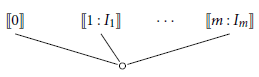
Every node s of C shares the same trace values $\mathrm{Tr}(s) = \{X_1^+, X_1^-, \ldots, X_n^+, X_n^-, R, G_0, \ldots, G_m\}$ . The ‘subtrees’ $[\![ 0 ]\!]$ and $[\![ \ell : I_\ell ]\!]$ each comprise of one or two buds whose companion is the root of $[\![ p ]\!]$ (drawn in white below). We refer to these buds by the names written above them. The $\mathcal{T}_\mathcal{A}$ -morphisms ‘decorating’ the subtrees’ edges are written next to them. For notational convenience, we often treat $\ell^+$ and $\ell^-$ as the label $\ell$ .

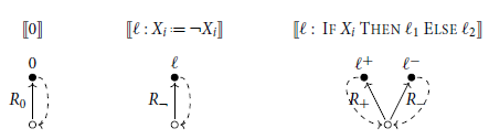
The morphisms are specified below. A dashed line between A and B indicates the pair (A, 0, B), a bold line the pair $(A, \alpha, B)$ and the absence of a connecting line between A and B the absence of all pairs (A, c, B). In $R_\neg$ , $\ell' = \ell + 1 \mod m + 1$ .

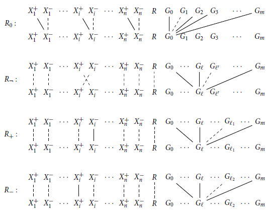
Write B for the set of names for buds of $[\![ p ]\!]$ , that is,

Any path through $[\![ p ]\!]$ corresponds to an infinite sequence $\ell \in B^\omega$ describing the sequence in which the buds of $[\![ p ]\!]$ are passed to generate said path. For this reason, we treat such sequences and paths $P : \mathcal{P}_C \to \mathcal{T}_\mathcal{A}$ interchangeably. The property central to the reduction is that if , then $[\![ p ]\!]$ does not satisfy the trace condition. Thus, sequences $\ell \in B^\omega$ representing unsuccessful runs will satisfy the trace condition. The various aspects of the trace maps given in Definition 7.2 can thus be reframed as ensuring certain conditions on such $\ell \in V^\omega$ .

We begin by showing that all sequences $\ell \in B^\omega$ $\ell \in B^\omega$ which eventually diverge or do not even adhere to the control structure of p have progressing traces through R or the $G_i$ s, respectively. For this, we define the control-graph of p as $G =(B, E)$ with

where, if , then pairs $(\ell_1, \ell_2)$ are included as $(\ell_1,\ell_2^+)$ and $(\ell_1,\ell_2^-)$ . For a sequence $\ell$ of labels from B (finite or infinite), $\ell$ is a path through G, writing $\ell \in G$ , if for each $i < \left|\ell\right|$ , $(\ell_i, \ell_{i +1}) \in E$ .

The only paths through $[\![ p ]\!]$ which remain unclassified are of the shape $u0u_10u_20u_30\ldots$ where each $u_i0$ describes a potential run of p which at least is a path through the control-graph of p. We continue by analysing the traces on the $X_i^\bullet$ along such potential runs. Consider a sequence $u = \ell_0 \ldots \ell_n \in B^{n + 1}$ and denote by $R^i$ the morphism in $[\![ p ]\!]$ from the root to the bud $\ell_i$ . In the following, we denote the trace map of the sequence u by $R_u:= R^{n - 1} \circ \ldots \circ R^0 \circ R_0$ .

With this classification of the potential runs, we can connect the trace condition on branches not covered by Lemma 7.1 to the runs of the program p.

-set finiteness of a trace category $\mathcal{T}$ does not entail PSPACE-hardness. For instance, consider a -set finite trace category $\mathcal{T}$ in which every path satisfies the trace condition and which thus makes checking it trivially O(1). This example also illustrates that $\omega$ -regularity of the trace condition of $\mathcal{T}$ does not entail PSPACE-hardness.

Remark 7.2. Theorem 7.1 does not directly imply that the proof checking of any concrete cyclic proof system is PSPACE-hard, even if its trace condition can be expressed in terms of $\mathcal{A}$ . Instead, Theorem 7.1 only proves that there exist ‘suitably small’ ACDs over $\mathcal{A}$ whose GTC satisfaction codes the termination of -programs. To extend this result to a concrete cyclic proof system, one must prove that for any -program p, there exists a ‘suitably small’ cyclic proof whose (compressed) ACD is $[\![ p ]\!]$ . Usually, this can be accomplished by finding formulas which can produce various traces. For example, for the variables, the following ‘trace gadgets’ are required:

To conclude PSPACE-completeness, it remains to show that proof checking for $\mathcal{T}_\mathcal{A}$ -ACDs is in PSPACE.