2. Bisimulation

The notion of bisimulation was introduced for automata in Park (Reference Park1981), extended by Milner to processes and then further modified to allow internal actions of those processes, Milner (Reference Milner1989). The classical notion is strong bisimulation, defined as a relation between labelled transition systems.

This definition characterises a labelled transition system as a function from labels to unlabelled transition systems. For each label, we get the transition system of actions with that label. By uncurrying F we get an equivalent definition as a function $A\times S \longrightarrow \operatorname{\mathcal P} S$ .

We can now define bisimulation.

• • for all ${s \stackrel{a}{\rightarrow}{s'}}$ , there is t’ such that ${t \stackrel{a}{\rightarrow}{t'}}$ and s’Rt’

• • and for all ${t \stackrel{a}{\rightarrow}{t'}}$ , there is s’ such that ${s \stackrel{a}{\rightarrow}{s'}}$ and s’Rt’.

3. Logical Relations

The idea behind logical relations is to take relations on base types, and extend them to relations on higher types in a structured way. The relations usually considered are binary, but they do not have to be. Even the apparently simple unary logical relations (logical predicates) are a useful tool. In this paper, we will be considering binary relations except for a few throwaway remarks. We will also keep things simple by just working with sets.

As an example, suppose we have a relation $R_0\subseteq S_0 \times T_0$ and a relation $R_1\subseteq S_1 \times T_1$ , then we can construct a relation $[R_0\rightarrow R_1]$ between the function spaces $[S_0\rightarrow S_1]$ and $[T_0\rightarrow T_1]$ . If $f:S_0\longrightarrow S_1$ and $g:T_0\longrightarrow T_1$ , then $f [R_0\rightarrow R_1] g$ if and only if for all s, t such that $s R_0 t$ , then $f(s) R_1 g(t)$ .

The significance of this definition for us is that it arises naturally out of a broader view of the structure. We consider categories of predicates and relations.

Pred also has a logical reading. We can take (P,A) as a predicate on the type A, and associate it with a judgement of the form $a:A \vdash P(a)$ (read “in the context $a:A$ , P(a) is a proposition”). A morphism $t \colon (a:A\vdash P(a)) \to (b:B\vdash Q(b))$ has two parts: a substitution $b\mapsto t(a)$ , and the logical consequence $P(a) \Rightarrow Q(t(a))$ (read “whenever P(a) holds, then so does Q(t(a))”).

Definition 4. The objects of the category ${{\sf Rel}}$ are triples $(R,A_1,A_2)$ where $A_1$ and $A_2$ are sets and R is a subset of $A_1\times A_2$ (a relation between $A_1$ and $A_2$ ). A morphism $(R,A_1,A_2) \longrightarrow (S,B_1,B_2)$ is a pair of functions $f_1 \colon A_1 \longrightarrow B_1$ and $f_2\colon A_2 \longrightarrow B_2$ such that $\forall a_1\in A_1, a_2\in A_2. (a_1,a_2)\in R \implies (f_1(a_1),f_2(a_2)) \in S$ . Identities and composition are inherited from ${\sf Set}\times{\sf Set}$ .

${\sf Rel}_n$ is the obvious generalisation of ${\sf Rel}$ to n-ary relations.

${\sf Pred}$ has a forgetful functor $p\colon {\sf Pred} \longrightarrow{\sf Set}$ , $p(P,A) = A$ , and similarly ${{\sf Rel}}$ has a forgetful functor $q\colon {\sf Rel}\longrightarrow{\sf Set}\times{\sf Set}$ , $q(R,A_1,A_2) = (A_1,A_2)$ , giving rise to two projection functors $\pi_0$ and $\pi_1$ ${\sf Rel}\longrightarrow{\sf Set}$ . These functors carry a good deal of structure and are critical to a deeper understanding of the constructions.

Moreover, both ${{\sf Pred}}$ and ${{\sf Rel}}$ are cartesian closed categories.

So the definition we gave above to extend relations to function spaces can be motivated as the description of the function space in a category of relations.

4. Covariant Powerset

We can do similar things with other type constructions. In particular, we can extend relations to relations between powersets.

• • for all $u\in U$ , there is a $v\in V$ such that uRv

• • and for all $v\in V$ , there is a $u\in U$ such that uRv

Again this arises naturally out of the lifting of a construction on ${\sf Set}$ to a construction on ${{\sf Rel}}$ . In this case, we have the covariant powerset monad, in which the unit $\eta: S \longrightarrow \operatorname{\mathcal P} S$ is $\eta s = \{ s\}$ , and the multiplication $\mu: \operatorname{\mathcal P}{}^2 S \longrightarrow \operatorname{\mathcal P} S$ is $\mu X = {\textstyle \bigcup} X$ .

There are two ways to motivate the definition we have just given. They both arise out of constructions for general monads, and in the case of monads on ${\sf Set}$ they coincide.

In ${{\sf Pred}}$ our powerset operator sends (Q,A) to $(\operatorname{\mathcal P}{Q}, \operatorname{\mathcal P} A)$ with the obvious inclusion. In ${{\sf Rel}}$ it almost sends $(R, A_1, A_2)$ to $(\operatorname{\mathcal P} R,\operatorname{\mathcal P}{A_1}, \operatorname{\mathcal P}{A_2})$ , where the “relation” is as follows: if $U\subseteq R$ (i.e. $U\in\operatorname{\mathcal P} R$ ) then U projects onto $\mathop{\pi_1} U$ and $\mathop{\pi_2} U$ . So for example, if R is the total relation on $\{0,1,2\}$ and $U=\{(0,1),(1,2)\}$ , then U projects onto $\{0,1\}$ and $\{1,2\}$ . The issue is that there are other subsets that project onto the same elements, e.g. $U'=\{(0,1),(1,1),(1,2)\}$ , and hence this association does not give a monomorphic embedding of $\operatorname{\mathcal P} R$ into $\operatorname{\mathcal P}{A_1}\times \operatorname{\mathcal P}{A_2}$ .

1. (1) there is $U\subseteq R$ such that $\mathop{\pi_1} U = P_1$ and $\mathop{\pi_2} U = P_2$

2. (2) for all $a_1\in P_1$ there is an $a_2\in P_2$ such that $a_1 R a_2$ and for all $a_2\in P_2$ there is an $a_1\in P_1$ such that $a_1 R a_2$ .

The latter is the Egli–Milner condition arising in the ordering on the Plotkin powerdomain, Plotkin (Reference Plotkin1976).

Thus for ${{\sf Rel}}$ we take the powerset of $(R,A_1,A_2)$ to be $(\operatorname{\mathcal P} R, \operatorname{\mathcal P}{A_1},\operatorname{\mathcal P}{A_2})$ , where $P_1 (\operatorname{\mathcal P} R) P_2$ if and only if $P_1$ and $P_2$ satisfy the equivalent conditions of Lemma 7.

Covariant powerset as the algebraic theory of complete $\vee$ -semilattices. This form of powerset does not characterise predicates on our starting point. Rather it characterises arbitrary collections of elements of it. To make this precise, consider the following formalisation of the theory of complete sup-semilattices. For each set X, we have an operation $\bigvee_X : L^X \longrightarrow L$ . In addition, for any $f:X\longrightarrow Y$ , composition with $L^f: L^Y\longrightarrow L^X$ is a substitution that takes an operation of arity X into one of arity Y. These operations satisfy the following equations:

1. (1) given a surjection $f: X\longrightarrow Y$ , $\bigvee_X \circ L^f = \bigvee_Y$ .

2. (2) given an arbitrary function $f: X\longrightarrow Y$ , $\bigvee_Y \circ (\lambda {y\in Y}. \bigvee_{f^{-1}\{y\}}\circ L^{i_y}) = \bigvee_X$ , where $i_y : f^{-1}\{y\} \longrightarrow X$ is the inclusion of $f^{-1}\{y\}$ in X.

The first axiom generalises idempotence and commutativity of the $\vee$ -operator. The second says that if we have a collection of sets of elements, take their $\bigvee$ ’s, and take the $\bigvee$ of the results, then we get the same result by taking the union of the collection and taking the $\bigvee$ of that. A particular case is that $\bigvee_\emptyset$ is the inclusion of a bottom element.

The fact that this theory includes a proper class of operators and a proper class of equations does not cause significant problems.

Suppose now that $f: A \longrightarrow B$ and B is a complete sup-semilattice. Then we have a map $f^{\ast} : \operatorname{\mathcal P} A \longrightarrow B$ defined by $f^{\ast} (X) = \bigvee_X (\lambda x\in X. f(x))$ . Equation (1) tells us that the operators $\bigvee_X$ are stable under isomorphisms of X, and hence we do not need to be concerned about that level of detail. Equation (2) now tells us that $f^{\ast}$ is a homomorphism. Moreover, if $X\subseteq A$ then in $\operatorname{\mathcal P} A$ , $X = \bigvee_X (\lambda x\in X. \{ x \})$ . Hence $f^{\ast}$ is the only possible homomorphism extending f. This gives the free property for $\operatorname{\mathcal P} A$ .

Moreover, if $f: (P,A) \longrightarrow (Q,B)$ where (Q,B) is a complete sup-semilattice, then we have $f^{\ast}: \operatorname{\mathcal P} A \longrightarrow B$ and (the restriction of) $f^{\ast}$ also maps $\operatorname{\mathcal P} P \longrightarrow Q$ . The proof is now essentially as in ${\sf Set}$ .

The proof in ${{\sf Rel}}$ is similar.

This type constructor has notable differences from a standard powerset. It (obviously) supports collecting operations of union, including a form of quantifier: $\bigcup : \operatorname{\mathcal P} \operatorname{\mathcal P} X \longrightarrow\operatorname{\mathcal P} X$ . However, it does not support either intersection or a membership operator.

1. (1) $\{a\} \operatorname{\mathcal P} R \{b\}$ and $\{a\} \operatorname{\mathcal P} R \{b'\}$ , but $\{a\}\cap\{a\} = \{a\}$ , while $\{b\}\cap\{b'\} = \emptyset$ , and it is not the case that $\{a\} \operatorname{\mathcal P} R \emptyset$ .

2. (2) aRb’ and $\{a\} \operatorname{\mathcal P} R \{b\}$ , but applying $\in$ to both left and right components of this gives different results: $\in (a,\{a\}) = \top$ , while $\in (b',\{b\}) = \bot$ .

Hence, $\cap$ and $\in$ are not parametric.

Despite the lack of these operations, this type constructor is useful to model non-determinism.

Covariant powerset in ${\sf Rel}$ using image factorisation. Suppose $Q\subseteq A$ , then $\operatorname{\mathcal P} Q\subseteq \operatorname{\mathcal P} A$ , and hence we can easily extend $\operatorname{\mathcal P}$ to Pred. However, if $R\subseteq A\times B$ , then $\operatorname{\mathcal P} R$ is a subset of $\operatorname{\mathcal P} (A\times B)$ , not $\operatorname{\mathcal P} A \times \operatorname{\mathcal P} B$ . The consequence is that $\operatorname{\mathcal P}$ does not automatically extend to ${\sf Rel}$ in the same way.

The second way to get round this is to note that we have projection maps $R \longrightarrow A$ and $R\longrightarrow B$ . Applying the covariant $\operatorname{\mathcal P}$ we get $\operatorname{\mathcal P} R \longrightarrow \operatorname{\mathcal P} A$ and $\operatorname{\mathcal P} R\longrightarrow \operatorname{\mathcal P} B$ , and hence a map $\phi: \operatorname{\mathcal P} R\longrightarrow (\operatorname{\mathcal P} A \times \operatorname{\mathcal P} B)$ . $\phi$ sends $U\subseteq R$ to

\begin{equation*}(\pi_A (U), \pi_B (U)) = (\{a\in A\ |\ \exists b\in B.\ (a,b)\in U\},\{b\in B\ |\ \exists a\in A.\ (a,b)\in U\})\end{equation*}

This map is not necessarily monic:

We therefore take its image factorization:

Using this definition, $\overline{\operatorname{\mathcal P} R}$ is

\begin{equation*}\{ (U,V) \in \operatorname{\mathcal P} A \times \operatorname{\mathcal P} B \ |\ \exists S\subseteq R.\ U=\pi_A S \wedge V = \pi_B S \}\end{equation*}

Now by Lemma 7 we have that this gives the same extension of covariant powerset to relations as the algebraic approach.

1. (1) $ U [\operatorname{\mathcal P} R] V $

2. (2) there is $S\subseteq R$ such that $\mathop{\pi_A} S = U$ and $\mathop{\pi_B} S = V$

3. (3) for all $a \in U$ there is an $b\in V$ such that a R b and for all $b \in V$ there is an $a \in U$ such that a R b.

5. Strong Bisimulation via Logical Relations

This now gives us the ingredients to introduce the notion of a logical relation between transition systems.

The following lemma is trivial to prove, but shows that we could take our uniform approach a step further to include relations on the alphabet of actions:

More significantly, we have

Conversely, if R is a strong bisimulation, then $\lambda as.\ \{s' | {s \stackrel{a}{\rightarrow}{s'}} \}$ and $\lambda at.\ \{t' | {t \stackrel{a}{\rightarrow}{t'}} \}$ are in the relation $[\mbox{ Id}_A \rightarrow [R\rightarrow \operatorname{\mathcal P} R]]$ . We have to check that if $a \mbox{ Id}_A a'$ and sRt then $\{s' | {s \stackrel{a}{\rightarrow}{s'}} \} \operatorname{\mathcal P} R \{t' | {t \stackrel{a'}{\rightarrow}{t'}} \}$ But if $a \mbox{ Id}_A a'$ , then $a=a'$ , so this reduces to $\{s' | {s \stackrel{a}{\rightarrow}{s'}} \} \operatorname{\mathcal P} R \{t' | {t \stackrel{a}{\rightarrow}{t'}} \}$ . Now Definition 6 says that we need to verify that:

• • for all ${s \stackrel{a}{\rightarrow}{s'}}$ , there is t’ such that ${t \stackrel{a}{\rightarrow}{t'}}$ and s’Rt’

• • and for all ${t \stackrel{a}{\rightarrow}{t'}}$ , there is s’ such that ${s \stackrel{a}{\rightarrow}{s'}}$ and s’Rt’.

This is precisely the bisimulation condition.

This means that we have rediscovered strong bisimulation as the specific notion of congruence for transition systems arising out of a more general theory of congruences between typed structures.

6. A Digression on Monads

The covariant powerset functor is an example of a monad, and the two approaches given to extend it to ${\sf Rel}$ at the end of Section 4 extend to general monads. In the case of monads on ${\sf Set}$ , they are equivalent.

${\sf Set}$ satisfies the Axiom Schema of Separation:

\begin{equation*} \forall v. \exists w. \forall x. [ x\in w \leftrightarrow x\in v \wedge \phi (x) ] \end{equation*}

This restricted form of comprehension says that for any predicate $\phi$ on a set v, there is a subset of v containing exactly the elements of v that satisfy $\phi$ . Since this is a set, we can apply functors to it.

Moreover, classical sets have the property that any monic whose domain is a non-empty set has a retraction. It follows that if m is such a monic, then Fm is also monic, where F is any functor.

This means that we can make logical predicates work for monads on ${\sf Set}$ , though there are limitations we will not go into here. We cannot necessarily do the same for monads on arbitrary categories, and we have already seen that this approach does not work for logical relations. In order to extend to logical relations, we have our algebraic and image factorisation approaches.

It is widely known that a large class of monads, monads where the functor preserves filtered (or more generally $\alpha$ -filtered) colimits correspond to algebraic theories. However, it is less commonly understood that arbitrary monads can be considered as being given by operations and equations, and that the property on the functor is really only used to reduce the collection of operations and equations down from a proper class to a set.

Let M be an arbitrary monad on ${\sf Set}$ , and $\theta: MB \longrightarrow B$ be an M-algebra. Let A be an arbitrary set, then any element of MA gives rise to an A-ary operation on B. Specifically, let t be an element of MA. An A-tuple of elements of B is given by a function $e: A\longrightarrow B$ , then we apply t to e by composing $\theta$ and Me and applying this to t: $(\theta\circ (Me))(t)$ . The monad multiplication can be interpreted as a mechanism for applying terms to terms, and we get equations from the functoriality of M and this interpretation of the monad operation.

We can look at models of this algebraic theory in the category ${\sf Rel}$ and interpret MR as the free model of this theory on R. That is the algebraic approach we followed for the covariant powerset $\operatorname{\mathcal P}$ .

Alternatively we can follow the second approach and use image factorisation.

Because of the particular properties of ${\sf Set}$ , monads preserve image factorisation.

1. (1) M preserves surjections: if $f: A\twoheadrightarrow B$ is a surjection from A onto B, then Mf is also a surjection.

2. (2) M preserves image factorisations: if

   
   is the image factorisation of $f = i\circ p$ , then
   
   is the image factorisation of Mf.

Given any monad M on ${\sf Set}$ , $MA\times MB$ is automatically an M-algebra with operation $\langle \mu_A\circ (M\pi_{MA}), \mu_B\circ (M\pi_{MB}) \rangle: M(MA\times MB) \longrightarrow MA\times MB$ . Moreover, $\overline{M R}$ is also an M-algebra.

Proof. This follows immediately from the fact that $\overline{M R}$ is an M sub-algebra of $MA\times MB$ .

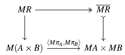
In the diagram above, the bottom horizontal composite is $\langle M\pi_A,M\pi_B\rangle$ , and the top composite is M applied to this. By Lemma 17, M preserves the image factorization in the bottom composite. It is easy to see that the outer rectangle commutes. It follows that there is a unique map across the centre making both squares commute, and hence that $\overline{MR}$ is an M sub-algebra of $MA\times MB$ .

The immediate consequence of this is that $\overline{MR}$ is the free M algebra on R in ${\sf Rel}$ and hence the two constructions by free algebra, and by direct image coincide in the case of monads on ${\sf Set}$ .

7. Monoids

Bisimulation is only one of the early characterisations of equivalence for labelled transition systems. Another was trace equivalence. That talks overtly about possible sequences of actions in a way that bisimulation does not. However, the sequences are buried in the recursive nature of the definition.

We extend our notion of transition from A to $A^{\ast}$ , in the usual way. The following is a simple induction:

• • for all ${s \stackrel{w}{\rightarrow}{s'}}$ , there is t’ such that ${t \stackrel{w}{\rightarrow}{t'}}$ and s’Rt’

• • and for all ${t \stackrel{w}{\rightarrow}{t'}}$ , there is s’ such that ${s \stackrel{w}{\rightarrow}{s'}}$ and s’Rt’.

In other words, we could have used sequences instead of single actions, and we would have got the same notion of bisimulation (but we would have had to work harder to use it).

Another way of looking at this is to observe that the set of transition systems on S, $[S\rightarrow \operatorname{\mathcal P} S]$ , carries a monoid structure. One way of seeing that is to note that $[S\rightarrow \operatorname{\mathcal P} S]$ is equivalent to the set of ${\textstyle \bigcup}$ -preserving endofunctions on $\operatorname{\mathcal P} S$ . Another is that it is the set of endofunctions on S in the Kleisli category for $\operatorname{\mathcal P}$ .

More concretely, the unit of the monoid is $\mbox{ id} = \eta = \lambda s. \{s\}$ , and the product is got from collection, $f_0\cdot f_1 = \lambda s. {\textstyle \bigcup}_{s'\in f_0(s)} f_1(s')$ .

Unsurprisingly, since this structure is essentially obtained from the monad, for any $R\subseteq S\times T$ , $[R\rightarrow \operatorname{\mathcal P} R]$ also carries the structure of a monoid, and the projections to $[S\rightarrow \operatorname{\mathcal P} S]$ and $[T\rightarrow \operatorname{\mathcal P} T]$ are monoid homomorphisms. This means that we could characterise strong bisimulations as relations R for which the monoid homomorphisms giving the transition systems lift to a monoid homomorphism into the relation.

8. Weak Bisimulation

The need for a different form of bisimulation arises when modelling processes. Processes can perform internal computations that do not correspond to actions that can be observed directly or synchronised with. In essence, the state of the system can evolve on its own. This is modelled by incorporating a silent $\tau$ action into the set of labels to represent this form of computation. Strong bisimulation is then too restrictive because it requires a close correspondence in the structure of the internal computations.

In order to remedy this, Milner introduced a notion of “weak” bisimulation. We follow the account given in Milner (Reference Milner1989), in which he refers to this notion just as “bisimulation”.

We write A (this is Milner’s Act), for the set of possible actions including $\tau$ and L for the actions not including $\tau$ . So $L = A - \{\tau\}$ and $A = L + \{\tau\}$ . If $w \in A^{\ast}$ , then we write $\hat{w}$ for the sequence obtained from w by deleting all occurrences of $\tau$ . So $\hat{w}\in L^{\ast}$ . For example, if $w=\tau a_0 a_1 \tau \tau a_0 \tau$ , then $\hat{w} = a_0 a_1 a_0$ , and if $w' = \tau\tau\tau$ , then $\hat{w'} = \epsilon$ , the empty string.

Definition 20. (Milner 1989) Let S be a labelled transition system for $A = L+\{\tau\}$ , and $v\in L^{\ast}$ , then

\begin{equation*} \mbox{${s \stackrel{v}{\rightarrow}{s'}}$ iff there is a $w\in A^{\ast} = (L+\{\tau\})^{\ast}$ such that $v=\hat{w}$ and ${s \stackrel{w}{\rightarrow}{s'}}$.} \end{equation*}

We can type $\rightarrow$ as $\rightarrow: [L^{\ast} \to [S\to\operatorname{\mathcal P} S]]$ , and we refer to it as the system derived from $\rightarrow$ .

Observe that ${s \stackrel{\epsilon}{\rightarrow}{s'}}$ corresponds to ${s \stackrel{\tau^{\ast}}{\rightarrow}{s'}}$ . It follows that $\rightarrow$ is not quite a transition system in the sense previously defined. If S is a labelled transition system for A, then the extension of $\rightarrow$ to $A^{\ast}$ gives a monoid homomorphism $A^{\ast} \longrightarrow [S\to\operatorname{\mathcal P} S]$ . However $\rightarrow$ preserves composition but not the identity. We have therefore only a semigroup homomorphism $L^{\ast} \longrightarrow [S\to\operatorname{\mathcal P} S]$ . This prompts the definition of a lax labelled transition system (Definition 31).

We now return to the classical definition of weak bisimulation from Milner (Reference Milner1989).

• • for all ${s \stackrel{a}{\rightarrow}{s'}}$ , there is t’ such that ${t \stackrel{a}{\rightarrow}{t'}}$ and s’Rt’

• • and for all ${t \stackrel{a}{\rightarrow}{t'}}$ , there is s’ such that ${s \stackrel{a}{\rightarrow}{s'}}$ and s’Rt’.

The combination of two different transition relations in this definition is ugly, but fortunately it is well known that we can clean it up by just using the derived relation.

• • for all ${s \stackrel{\overline{a}}{\rightarrow}{s'}}$ , there is t’ such that ${t \stackrel{\overline{a}}{\rightarrow}{t'}}$ and s’Rt’

• • and for all ${t \stackrel{\overline{a}}{\rightarrow}{t'}}$ , there is s’ such that ${s \stackrel{\overline{a}}{\rightarrow}{s'}}$ and s’Rt’

where for $x \in L$ , $\overline x$ is “x” seen as a one-letter word, and for $x=\tau$ , $\overline x = \epsilon$ .

We can now extend as before to words in $L^{\ast}$ .

• • for all ${s \stackrel{v}{\rightarrow}{s'}}$ , there is t’ such that ${t \stackrel{v}{\rightarrow}{t'}}$ and s’Rt’

• • and for all ${t \stackrel{v}{\rightarrow}{t'}}$ , there is s’ such that ${s \stackrel{v}{\rightarrow}{s'}}$ and s’Rt’.

Note that we can restrict the underlying alphabet from $A = L+\{\tau\}$ to L because $\epsilon\in L^{\ast}$ is playing the role of $\tau\in A$ .

This now looks very similar to the situation for strong bisimulation. But as we have noted above, there is a difference. Previously our transition system was given by a monoid homomorphism $A^{\ast} \longrightarrow [S\rightarrow \operatorname{\mathcal P} S]$ . Here the identity is not preserved and we only have a homomorphism of semi-groups.

In the following sections we present different approaches to understanding weak transition systems.

9. Weak Bisimulation through Saturation

For this section, we enrich our setting. For any S, $\operatorname{\mathcal P} S$ has a natural partial order, and hence so do the transition systems on any set S, given by the inherited partial order on $A \to [S\to \operatorname{\mathcal P} S]$ .

If $A=L+\{\tau\}$ , where $\tau$ is an internal (silent) action, then we shall refer to these as labelled transition systems with internal action and write the partial order as $(L{+}\tau)$ -TS.

The notion of weak bisimulation applies to transition systems with internal action, while strong bisimulation applies to arbitrary transition systems. Our aim is to find a systematic way of deriving the notion of weak bisimulation from strong.

In the following definition, we make use of the fact that $[S\to \operatorname{\mathcal P} S]$ is a monoid, as noted in Section 7.

1. (1) $\mbox{ id} \leq F(\tau)$ and $F(\tau).F(\tau) \leq F(\tau)$ and

2. (2) for all $a\in L$ , $F(\tau).F(a).F(\tau) \leq F(a)$

We write L-Sat-TS for the full subcategory of saturated transition systems with internal actions.

These conditions are purely algebraic, and so can easily be interpreted in more general settings than ${\sf Set}$ .

Note that some of the inequalities are, in fact, equalities:

\begin{equation*}F(\tau) = F(\tau) . \mbox{ id} \leq F(\tau).F(\tau) \leq F(\tau)\end{equation*}

hence $F(\tau).F(\tau) = F(\tau)$ . Similarly $F(a) = \mbox{ id}.F(a).\mbox{ id} \leq F(\tau).F(a).F(\tau) \leq F(a)$ , therefore $F(\tau).F(a).F(\tau)=F(a)$ .

Moreover, if we look at the partial order consisting of unlabelled transition systems on a set S, then the fact that the monoid multiplication preserves the partial order means that $([S\to \operatorname{\mathcal P} S], . , \mbox{ id})$ is a monoidal category. Condition 26.1 says precisely that $F(\tau)$ is a monoid in this monoidal category, and Condition 26.2 that F(a) is an $(F(\tau),F(\tau))$ -bimodule.

The notions of weak and strong bisimulation coincide for saturated transition systems.

• • $a\neq\tau$ : Then, by definition of ${ \stackrel{a}{\Rightarrow}{}}$ , we have $t ({ \stackrel{\tau{}}{\rightarrow}{^{\ast}}}) { \stackrel{a}{\rightarrow}{}} ({ \stackrel{\tau}{\rightarrow}{}})^{\ast} t'$ . But since F is saturated, this implies ${t \stackrel{a}{\rightarrow}{t'}}$ as required.

• • $a=\tau$ : Then $t ({ \stackrel{\tau}{\rightarrow}{}})^{\ast} t'$ , and again since F is saturated, this implies ${{t} \stackrel{\tau}{\rightarrow}{t'}}$ .

Hence, we have ${t \stackrel{a}{\rightarrow}{t'}}$ and tRt’. The symmetric case is identical, so R is a strong bisimulation.

Given any transition system with internal action, there is a least saturated transition system containing it.

• • $\overline{F}(\tau) = F(\tau)^{\ast}$

• • $\overline{F}(a) = \overline{F}(\tau).F(a).\overline{F}(\tau)$ ( $a\neq\tau$ )

1. (1) R is a weak bisimulation between F and G

2. (2) $\overline{F}$ and $\overline{G}$ are in the appropriate logical relation: $(\overline{F},\overline{G})\in[\mbox{ Id}_{L+\{\tau\}}\to [R\to\operatorname{\mathcal P} R]]$

3. (3) R is the state space of a saturated transition system in ${\sf Rel}$ whose first projection is $\overline{F}$ and whose second is $\overline{G}$ .

The consequence of this is that we now have two separate ways of giving semantics to transition systems with inner actions. Given $F\colon(L+\tau)\longrightarrow[S\to\operatorname{\mathcal P} S]$ , we can just take F as a transition system. If we then apply the standard logical relations framework to this definition, we get that two such, F and G, are related by the logical relation $[\mbox{ Id}_{(L+\tau)} \to [R\to\operatorname{\mathcal P} R]]$ if and only if R is a strong bisimulation between F and G. If instead we take the semantics to be $\overline{F}$ , typed as $\overline{F}:(L+\tau)\longrightarrow[S\to\operatorname{\mathcal P} S]$ , then $\overline{F}$ and $\overline{G}$ are related by the logical relation $[\mbox{ Id}_{(L+\tau)} \to [R\to\operatorname{\mathcal P} R]]$ if and only if R is a weak bisimulation between F and G.

10. Lax Transition Systems

Saturated transition systems still include explicit $\tau$ -actions even though these are supposed to be internal actions only indirectly observable. We can however avoid $\tau$ ’s appearing explicitly in the semantics by giving a relaxed variant of the monoid semantics.

We recall that for an arbitrary set of action labels A, the set of A-labelled transition systems $A\longrightarrow[S\to\operatorname{\mathcal P} S]$ is isomorphic to the set of monoid homomorphisms $A^{\ast}\longrightarrow[S\to\operatorname{\mathcal P} S]$ , and moreover that for any transition systems F and G and relation $R\subseteq S\times T$ , F is related to G by $[{\mbox{ Id}_A}\to[R\to\operatorname{\mathcal P} R]]$ iff F is related to G as monoid homomorphism by $[{\mbox{ Id}_{A^{\ast}}}\to [R\to\operatorname{\mathcal P} R]]$ iff R is a strong bisimulation between F and G.

We can model transition systems with internal actions similarly, by saying what transitions correspond to sequences of visible actions. The price we pay is that, since $\tau$ is not visible, we have genuine state transitions corresponding to the empty sequence. We no longer have a monoid homomorphism.

1. (1) $\mbox{ id}\leq F(\epsilon)$ (reflexivity)

2. (2) $F(vw) = F(v).F(w)$ (composition)

1. (1) $\hat{F} (\epsilon) = F(\tau)^{\ast}$

2. (2) $\hat{F} (a) = F(\tau)^{\ast}. F(a). F(\tau)^{\ast}$ , for any $a\in L$ .

3. (3) $\hat{F} (vw) = \hat{F} (v) . \hat{F} (w)$ .

It is trivial that $\hat{F}$ is a lax transition system.

We have reproduced the derived transition system.

Note that if G is a lax transition system, then G(w) depends only on $G(\epsilon)$ and the G(a), all other values are determined by composition. Note also that if F is saturated, then $\hat{F}(\epsilon) = F(\tau)$ and $\hat{F}(a) = F(a)$ .

We can also go the other way. Given a lax transition system, $F:L^{\ast}\longrightarrow [S\to\operatorname{\mathcal P} S]$ , then we can define a transition system with inner action: $\check{F}:(L+\{\tau\})\longrightarrow [S\to\operatorname{\mathcal P} S]$ where

• • $\check{F} (\tau) = F(\epsilon)$

• • $\check{F} (a) = F(a)$

One way of looking at this is that a lax transition system is just a saturated one in thin disguise. But from our perspective it gives us a different algebraic semantics for transition systems with inner action that can also be made to account for weak bisimulation, and this time the $\tau$ actions do not appear in the formal statement.

1. (1) R is a weak bisimulation between F and G

2. (2) $(\hat{F},\hat{G})\in [\mbox{ Id}_{L^{\ast}}\to [R\to\operatorname{\mathcal P} R]]$

3. (3) R is the state space of a lax transition system in ${\sf Rel}$ whose first projection is $\hat{F}$ and whose second is $\hat{G}$ .

11. (Semi-)Branching Bisimulations

In this section, we shall always consider two labelled transition systems $F \colon (L + \{\tau\}) \longrightarrow [ S \to \operatorname{\mathcal P} S]$ and $G \colon (L + \{\tau\}) \longrightarrow [T \to \operatorname{\mathcal P} T]$ with an internal action $\tau$ . We begin by introducing the following notation: we say that $x \overset{\tau^*}{\to} y$ , for x and y in S (or in T) if and only if there is a finite, possibly empty, sequence of $\tau$ actions

\begin{equation*}x \overset \tau \to \cdots \overset \tau \to y;\end{equation*}

if the sequence is empty, then we require $x = y$ .

We now recall the notion of branching bisimulation, which was introduced in van Glabbeek and Weijland (Reference van Glabbeek and Weijland1996).

• • $s \overset{a}{\to} {s'}$ implies $\bigl( (\exists t_1,t_2 \in T \ldotp t \overset {\tau^*} \to {t_1} \overset a \to {t_2} \land s R t_1 \land s' R t_2) \text{ or } ( a = \tau \land s' R t) \bigr)$ ,

• • $t \overset{a}{\to} {t'}$ implies $\bigl( (\exists s_1,s_2 \in S \ldotp s \overset {\tau^*} \to {s_1} \overset a \to {s_2} \land s_1 R t \land s_2 R t') \text{ or } ( a = \tau \land s R t') \bigr)$ .

We show how branching bisimulation is also an instance of logical relation between appropriate derived versions of F and G.

Definition 38. The branching saturation of F, denoted by $\overline{F}^b$ , is a function

\begin{equation*} \overline{F}^b \colon (L+\{\tau\}) \longrightarrow [ S \to \operatorname{\mathcal P} {\!(S \times S)}] \end{equation*}

defined as follows. Given $s \in S$ and $a \in L + \{\tau\}$ ,

\begin{equation*} \overline{F}^b a s = \{ (s_1,s_2) \in S \times S \mid (s \overset {\tau^*} \to s_1 \overset a \to s_2) \text{ or } (a = \tau \text{ and } s=s_1=s_2) \}. \end{equation*}

Suppose then that R is a branching bisimulation, consider s R t and take $(s_1,s_2) \in \overline{F}^b a s$ . We have two possible cases to discuss: $a = \tau \text{ and } s=s_1=s_2$ , or $s \overset {\tau^*} \to s_1 \overset a \to s_2$ . In the first case, consider the pair (t,t): this clearly belongs to $\overline{G}^b a t$ . In the second case, we are in the following situation:

If $\tau^*$ is the empty list, then $s=s_1$ , hence $s_1 R t$ : by definition of branching bisimulation, there are indeed $t_1$ and $t_2$ such that:

hence $(t_1,t_2) \in \overline{G}^b a t$ . If $\tau^*=\tau^n$ , with $n \ge 1$ , then by Remark 37 applied to every $\tau$ in the list $\tau^*$ , there exists t’ in T such that $t \overset{\tau^*}{\to} t'$ and $s_1 R t'$ . Now apply again the definition of branching bisimulation for s R t’: we have that there are $t_1$ and $t_2$ in T such that:

hence $(t_1,t_2)\in \overline{G}^b a t$ . This proves that if R is a branching bisimulation, then $(\overline{F}^b, \overline{G}^b) \in [\mbox{ Id}_{L+\{\tau\}} \to [R \to \operatorname{\mathcal P}{(R \times R)}]]$ .

Conversely, suppose $(\overline{F}^b, \overline{G}^b) \in [\mbox{ Id}_{L+\{\tau\}} \to [R \to \operatorname{\mathcal P}{(R \times R)}]]$ and that we are in the following situation:

Then we have $(s,s') \in \overline{F}^b a s$ , because indeed $s \overset {\tau^*} \to s \overset a \to s'$ . By definition of the relation $\operatorname{\mathcal P}{\!(R \times R)}$ , there exists $(t_1,t_2) \in \overline{G}^b a t$ such that $s R t_1$ and $s' R t_2$ . It is immediate to see that this is equivalent to the condition required by Definition 36, hence R is in fact a branching bisimulation.

In van Glabbeek and Weijland (Reference van Glabbeek and Weijland1996) also a weaker notion of branching bisimulation was introduced, which we recall now.

• • $s \overset{a}{\to} {s'}$ implies $\bigl( (\exists t_1,t_2 \in T \ldotp t \overset {\tau^*} \to {t_1} \overset a \to {t_2} \land s R t_1 \land s' R t_2)$ or $( a = \tau \land \exists t' \in T \ldotp {t \overset {\tau^*} \to t'} \land s R t' \land s' R t') \bigr)$ ,

• • $t \overset{a}{\to} {t'}$ implies $\bigl( (\exists s_1,s_2 \in S \ldotp s \overset {\tau^*} \to {s_1} \overset a \to {s_2} \land s_1 R t \land s_2 R t')$ or $( a = \tau \land \exists s' \in S \ldotp {s \overset {\tau^*} \to s'} \land s' R t \land s' R t') \bigr)$ .

Every branching bisimulation is also semi-branching, but the converse is not true. The difference between branching and semi-branching bisimulation is in what is allowed to happen in the $\tau$ -case. Indeed, if $s \overset{\tau}{\to} s'$ and sRt, in the branching case it must be that either also s’Rt, or t can “evolve” into $t_1$ , for $sRt_1$ , by means of zero or more $\tau$ actions, and then $t_1$ has to evolve into a $t_2$ via a $\tau$ action with $s' R t_2$ . In the semi-branching case, t is always allowed to evolve into t’ with zero or more $\tau$ steps, as long as s is still related to t’, as well as s’ R t’. Figure 1 shows this in graphical terms.

Figure 1. Difference between branching (left) and semi-branching (right) case for $\tau$ actions.

We can prove a result analogous to Theorem 39 for semi-branching bisimulations. To do so, we introduce an appropriate derived version of a labelled transition system $F \colon (L+\{\tau\}) \longrightarrow [S \to \operatorname{\mathcal P}{\!(S\times S)}]$ .

Definition 41. The semi-branching saturation of F, denoted by $\widetilde{F}$ , is a function

\begin{equation*} \widetilde{F} \colon (L+\{\tau\}) \longrightarrow [ S \to \operatorname{\mathcal P}{\!(S \times S)}] \end{equation*}

defined as follows. Given $s \in S$ and $a \in L+\{\tau\}$ ,

\begin{equation*} \widetilde{F} a s = \{ (s_1,s_2) \in S \times S \mid (s \overset {\tau^*} \to s_1 \overset a \to s_2) \text{ or } (a = \tau \text{ and } s_1 = s_2 \text{ and } s \overset {\tau^*} \to s_1 \}. \end{equation*}

Notice that Remark 37 continues to hold for semi-branching bisimulations too.

12. The Almost-Monad

In Section 7, we observed that $[S \to \operatorname{\mathcal P}{S}]$ enjoys a monoid structure inherited from the monadicity of the covariant powerset $\operatorname{\mathcal P}{}$ . Sadly, we cannot say quite the same for $[S \to \operatorname{\mathcal P}{(S \times S)}]$ . Indeed, consider the functor $T(A)=\operatorname{\mathcal P}{(A \times A)}$ :

where $\operatorname{\mathcal P}{(f\times f)}(S) = \{\bigl(f(x),f(y)\bigr) \mid (x,y) \in S\}$ . We can define two natural transformations $\eta \colon \mbox{ Id}_{\sf Set} \longrightarrow T$ and $\mu \colon T^2 \longrightarrow T$ as follows: $\eta_A (a) = \{(a,a)\}$ and

It is not difficult to see that $\eta$ and $\mu$ are indeed natural, and that the following square commutes for every set A:

However, although the left triangle in the following diagram commutes, the right one fails to do so in general:

Indeed, given $S \subseteq A \times A$ , it is true that $S \cup S = S$ , but

\begin{equation*}\mu_A\bigl(T\eta_A(S)\bigr) = \mu_A\Bigl( \left\{ \bigl( \{(x,x)\}, \{(y,y)\} \bigr) \mid (x,y) \in S \right\} \Bigr) = \bigcup_{(x,y)\in S} \bigl( \{(x,x)\} \cup \{(y,y)\} \bigr) \ne S.\end{equation*}

This means that $(T,\eta,\mu)$ falls short of being a monad: it is only a “left-semi-monoid” in the category of endofunctors and natural transformations on ${\sf Set}$ , in the sense that $\eta$ is only a left unit for the multiplication $\mu$ .

One can go further, and build up the “Kleisli non-category” associated to $(T,\eta,\mu)$ , following the usual definition for Kleisli category of a (proper) monad, where morphisms $A \longrightarrow B$ are functions $A \longrightarrow \operatorname{\mathcal P}{(B \times B)}$ , and composition of $f \colon A \longrightarrow \operatorname{\mathcal P}{(B \times B)}$ and $g \colon B \longrightarrow \operatorname{\mathcal P}{(C \times C)}$ is the composite in ${\sf Set}$ :

This composition law has $\eta$ as a left-but-not-right identity. Whereas the set of endomorphisms on A in the Kleisli category of a proper monad is always a monoid with the multiplication defined as the composition above, here we get that $[A \to \operatorname{\mathcal P}{(A \times A)}]$ is only a left-semi-monoid.

We can define a partial order on $[A \to \operatorname{\mathcal P}{(A \times A)}]$ in a canonical way, by setting $f \le g$ if and only if for all $a \in A$ $f(a) \subseteq g(a)$ ; by doing so, we can regard $[A \to \operatorname{\mathcal P}{(A \times A)}]$ as a category. The multiplication $f \cdot g \colon A \longrightarrow \operatorname{\mathcal P}{(A \times A)}$ , defined as $f \cdot g (a)=\bigcup_{(x,y)\in f(a)} (g(x) \cup g(y))$ , preserves the partial order, therefore $[A \to \operatorname{\mathcal P}{(A \times A)}]$ is a “left-semi-monoidal” category.

13. Branching and Semi-branching Saturated Systems

In this section, we investigate the properties of $\overline{F}^b(\tau)$ and $\widetilde{F}(\tau)$ as elements of $[S \to \operatorname{\mathcal P}{(S \times S)}]$ , for $F \colon (A+\{\tau\}) \longrightarrow [S \to \operatorname{\mathcal P}{(S \times S)}]$ , to explore whether it is possible to define an appropriate notion of branching or semi-branching saturated systems, where strong and branching (or semi-branching) bisimulations are the same, cf. weak case in Sections 9 and 10.

Let now $(x,y) \in (\overline{F}^b(\tau) \cdot \overline{F}^b(\tau))(s) = \bigcup_{(s_1,s_2) \in \overline{F}^b \tau (s)} \bigl( \overline{F}^b\tau (s_1) \cup \overline{F}^b \tau(s_2) \bigr)$ : we want to check whether $(x,y) \in \overline{F}^b \tau (s)$ . Suppose that $(x,y) \in \overline{F}^b \tau (s_1)$ for some $(s_1,s_2) \in \overline{F}^b \tau (s)$ . Then we are in one of the following four situations:

In cases 1 and 2, we can conclude that

, while in case 4 we get $s=x=y$ , hence $(x,y) \in \overline{F}^b \tau (s)$ . However, if in case 3 we are in the situation whereby $s \ne s_1$ , then $(x,y)\notin \overline{F}^b \tau (s)$ , as it is neither the case that $s=x=y$ nor

It turns out, however, that the semi-branching saturation of F behaves much better than $\overline{F}^b$ .

Proof. Again, it is immediate to see that $\eta_S \le \widetilde{F}(\tau)$ , because

for any s, given that $\tau^*$ can be the empty list of $\tau$ ’s.

Now we prove that $\widetilde{F} (\tau) \cdot \widetilde{F} (\tau) \le \widetilde{F}(\tau)$ . Let $s \in S$ and $(x,y) \in (\widetilde{F} (\tau) \cdot \widetilde{F} (\tau))(s)$ . Then there exists a pair $(s_1,s_2) \in \widetilde{F} \tau (s)$ such that $(x,y) \in \widetilde{F} \tau (s_1)$ or $(x,y) \in \widetilde{F} \tau (s_2)$ . Suppose that $(x,y) \in \widetilde{F} \tau (s_1)$ , then we are in one of the four following cases:

In every case, we can conclude that $(x,y) \in \widetilde{F} \tau (s)$ . Thus $\widetilde{F}(\tau)$ is a left-semi-monoid.

Finally, we show that $\widetilde{F} (\tau) \cdot \widetilde{F} (a) \le \widetilde{F}(a)$ for all $a \in A$ . Let $s \in S$ and consider $(x,y) \in (\widetilde{F} \tau \cdot \widetilde{F} a)(s)$ . Then $(x,y) \in \widetilde{F} a (s_1)$ or $(x,y) \in \widetilde{F} a (s_2)$ for some $(s_1,s_2) \in \widetilde{F} \tau (s)$ . In the first case (and similarly for the second), it is

and in both cases we have $(x,y) \in \widetilde{F} a (s)$ , as required.

Remark 45. It is not true, in general, that $\widetilde{F} a \cdot \widetilde{F} \tau \le \widetilde{F} a$ . Indeed, consider $s \in S$ and $(x,y) \in (\widetilde{F} a \cdot \widetilde{F} \tau)(s)=\bigcup_{(s_1,s_2) \in \widetilde{F} a (s)} (\widetilde{F} \tau (s_1) \cup \widetilde{F} \tau (s_2))$ . Then the following is one of four possible scenarios:

where it is clear that $(x,y)\notin \widetilde{F} a (s)$ .

14. The Category $\sf Meas$

Our next goal is to discuss bisimulation for continuous Markov processes (see de Vink and Rutten Reference de Vink and Rutten1999; Panangaden Reference Panangaden2009). In order to do this, we need to step cautiously out of the world of sets and functions, and into that of measurable spaces and measurable functions.

We recall that a measurable space $(X,\Sigma)$ is a set X equipped with a $\sigma$ -algebra, $\Sigma$ , the algebra of measurable sets. A measurable function $f \colon (X,\Sigma_X) \longrightarrow(Y,\Sigma_Y)$ is a function $f\colon X \longrightarrow Y$ such that if U is a measurable set of $(Y,\Sigma_Y)$ , then $f^{-1} U$ is a measurable set of $(X,\Sigma_X)$ . Together these form a category, $\sf Meas$ .

Lemma 47.

$\sf Meas$ has coequalisers. If

is a pair of parallel measurable functions, then their coequaliser is $E: (Y,\Sigma_Y)\longrightarrow (Y/{\sim},\overline\Sigma)$ , where $\sim$ is the equivalence relation on Y generated by $fx\sim gx$ , and $\overline\Sigma$ is the largest $\sigma$ -algebra on $Y/{\sim}$ making $Y\longrightarrow Y/{\sim}$ measurable, i.e. $\overline\Sigma = \{ V \ |\ e^{-1} V \in \Sigma_Y \}$ .

However, $\sf Meas$ is not regular because the pullback of a regular epi is not necessarily regular, as exhibited by this counterexample:

The consequence of this is that $\sf Meas$ has all the apparatus to construct a relational calculus, but that calculus does not have all the properties we expect. Specifically it is not an allegory. Accordingly, when we want to construct logical relations on $\sf Meas$ , we will take the measurable spaces as structures in ${\sf Set}$ and use the constructs in ${\sf Set}$ .

15. Probabilistic Bisimulation

We follow the standard approach by defining a continuous Markov process to be a coalgebra for the Giry functor. For simplicity, we will work with unlabelled processes.

• • $\Pi X$ is the set of sub-probability measures on $(X,\Sigma_X)$ .

• • $\Pi\Sigma_X$ is the least $\sigma$ -algebra on $\Pi X$ such that for every $U\in\Sigma_X$ , $\lambda\pi. \pi(U)$ is measurable.

If $f \colon (X,\Sigma_X) \longrightarrow (Y,\Sigma_Y)$ is a measurable function, then $\Pi f (\pi) = \lambda V\in\Sigma_Y. \pi (f^{-1} V)$ . $\Pi$ forms part of a monad in which the unit maps a point x to the Dirac measure for x, and the multiplication is defined by integration, Giry (Reference Giry1982).

There are now two similar, but slightly different approaches to defining the notion of a probabilistic bisimulation. Panangaden (Reference Panangaden2009) follows Larsen and Skou’s original definition for the discrete case. This begins by enabling a state space reduction for a single process and generates a notion of bisimulation between processes as a by-product. The second is the standard notion of bisimulation of coalgebras, as described in Rutten (Reference Rutten2000).

We begin with Panangaden’s extension of the original definition of Larsen and Skou, Panangaden (Reference Panangaden2009), Larsen and Skou (Reference Larsen and Skou1991).

We note that the R-closed measurable sets are exactly those inducing the $\sigma$ -algebra on $S/R$ , and hence that this definition of equivalence corresponds to the ability to quotient the state space to give a continuous Markov process on $S/R$ .

This definition assumes that R is total. However, that is not essential. We could formulate it for relations that are symmetric and transitive, but not necessarily total (partial equivalence relations). In this case, we have a correspondence with subquotients of the coalgebra. We do, however, have to be careful that the domain of R is a well-defined sub-algebra.

Panangaden goes on to define a bisimulation between two coalgebras. We simplify his definition as we do not consider specified initial states.

Given a binary relation R between S and T, we extend R to a binary relation on the single set $S+T$ . In order to apply the previous definition, we will want the equivalence relation on $S+T$ generated by R.

Now $(S+T)\times (S+T) = (S\times S) + (S\times T) + (T\times S) + (T\times T)$ , and each of these components has a simple relation derived from R, specifically $R{R}^\circ $ , R, ${R}^\circ$ and ${R}^\circ R$ .

Secondly, given continuous Markov processes F on S and G on T we can define their sum $F+G$ on $S+T$ :

\begin{equation*}(F+G) x U = \begin{cases}Fx(U \cap S) & \text{if $x \in S$} \\Gx(U \cap T) & \text{if $x \in T$}\end{cases}\end{equation*}

We can now make a definition that seems to us to contain the essence of Panangaden’s approach:

Note that any such relation will be z-closed. Given that $R^{\ast}$ must be total, it also induces an isomorphism between quotients of the continuous Markov processes.

This definition corresponds exactly to what we get by taking the obvious logical relations approach.

Logical relations of continuous Markov Processes. Given a measurable space $(S,\Sigma_S)$ , we treat the $\sigma$ -algebra $\Sigma_S$ as a subset of the function space $[S\to 2]$ , and use the standard mechanisms of logical relations in ${\sf Set}$ to extend a relation $R\subseteq S\times T$ between two measurable spaces to a relation $R_\Sigma$ between $\Sigma_S$ and $\Sigma_{T}$ : $UR_\Sigma V$ if and only if $\forall s,t. sRt \implies (s\in U \iff t\in V)$ .

Unpacking the definition of the Giry functor, a Giry coalgebra structure on the measurable space $(S,\Sigma_S)$ has type $S\longrightarrow [\Sigma_S \to [0,1]]$ , or equivalently $S \times \Sigma_S \longrightarrow [0,1]$ , where for the purposes of defining logical relations we regard $\Sigma_S$ as a subset of $[S\to 2]$ . We again apply the standard machinery to this.

The following lemmas follow readily from the definitions.

So logical relations capture both the concept of strong probabilistic bisimulation (given that the candidate relations are restricted in nature), and the concept of homomorphism of systems. But they do not capture everything.

$\Pi$

-bisimulation. Recall from Rutten (Reference Rutten2000) that for a functor $H \colon \sf C \longrightarrow \sf C$ and two H-coalgebras $f \colon A \longrightarrow HA$ and $g \colon B \longrightarrow HB$ , an H-bisimulation between f and g is a H-coalgebra $h \colon C \longrightarrow HC$ together with two coalgebra-homomorphisms $l \colon C \longrightarrow A$ and $r \colon C \longrightarrow B$ , that is, it is a span in the category of coalgebras for H:

where the above diagram is required to be commutative.

It is implicit in this definition that a bisimulation includes a coalgebra structure, and is not simply a relation. Where the functor H corresponds to a traditional algebra generated by first-order terms and equations, the algebraic structure on the relation is unique. But that is not the case here.

1. (1) a “two independent copies” structure given by

   \begin{equation*}FF (s,s') (U,U') = (F s U) \times (F s' U')\end{equation*}

2. (2) a “two observations of a single copy” structure given by

   \begin{equation*} F^2 (s,s') (U,U') = \begin{cases} F s (U\cap U') & \text{if $s = s'$} \\ F s U \times F s' U' & \text{ if $s \ne s'$} \end{cases} \end{equation*}

Example 64. More specifically, consider the process t modelling a single toss of a fair coin. This can be modelled as a process with three states, $C=\{S,H,T\}$ : Start (S), Head tossed (H) and Tail tossed (T). From S we move randomly to one of H and T and then stay there. The transition matrix is given below. This is a discrete process, and we take all subsets to be measurable.

\begin{equation*}t\mbox{ is given by} \quad\begin{array}{c|ccc} & S & H & T \\ \hline S & 0 & 0.5 & 0.5 \\ H & 0 & 1 & 0\\ T & 0 & 0 & 1 \end{array} \end{equation*}

Now consider the state space $C\times C$ . We define two different process structures on this. The first, $t^{*}$ , is simply the product of the two copies of C. The transition matrix for this is the tensor of the transition matrix for C with itself: the pairwise product of the entries. This represents the process of two independent tosses of a coin.

\begin{equation*}t^{*}\mbox{ is given by } \quad\begin{array}{c|*{9}{c}} & SS & HH & TT & HT & TH & SH & HS & ST & TS \\ \hline SS & 0 & 0.25 & 0.25 & 0.25 & 0.25 & 0 & 0 & 0 & 0 \\ HH & 0 & 1 & 0 & 0 & 0 & 0 & 0 & 0 & 0\\ TT & 0 & 0 & 1 & 0 & 0 & 0 & 0 & 0 & 0\\ HT & 0 & 0 & 0 & 1 & 0 & 0 & 0 & 0 & 0\\ \ldots\\ TS & 0 & 0 & 0.5 & 0 & 0.5 & 0 & 0 & 0 & 0 \end{array} \end{equation*}

The second, $t^{+}$ is identical except for the first row:

\begin{equation*}t^{+}\mbox{ is given by } \quad\begin{array}{c|*{9}{c}} & SS & HH & TT & HT & TH & SH & HS & ST & TS \\ \hline SS & 0 & 0.5 & 0.5 & 0 & 0 & 0 & 0 & 0 & 0 \\ \ldots \end{array} \end{equation*}

This is motivated by the process of two observers watching a single toss of a coin.

The projections are homomorphisms for both these structures. For example, the first projection is a homomorphism for $t^{+}$ because for each I, J, K:

\begin{equation*} t I \{K\} = \sum_L t^{+} IJ \{KL\} \end{equation*}

This means that in order to establish that a relation is a $\Pi$ -bisimulation, we have to define a structure and prove the homomorphisms, and not simply validate some closure conditions.

Moreover, in contrast to the case for first-order theories, this non-uniqueness of algebra structures implies that we cannot always reduce spans of homomorphisms to relations.

We now show that, despite these issues, $\Pi$ -bisimulations give rise to logical relations.

Theorem 66. Suppose

is a $\Pi$ -bisimulation between the continuous Markov processes F and G. Let $R \subseteq S \times T$ be the relation which is the image of $\langle l,r\rangle \colon P \longrightarrow S\times T$ , i.e. sRt iff $\exists p. lp=s \wedge rp=t$ . Then R is a logical relation between F and G.

We begin by showing that $l^{-1}U = r^{-1}V$ . Suppose $p\in P$ , then (lp)R(rp), and hence $p\in l^{-1} U$ iff $lp\in U$ iff $rp\in V$ (since $UR_\Sigma V$ ) iff $p\in r^{-1}V$ . Hence $l^{-1}U = r^{-1}V$ , as required.

Now, since sRt, there is a p such that $lp=s$ and $rp=t$ . Then

\begin{align*} F(s)(U) &= H p (l^{-1} U) &\text{because \textit{l} is a $\Pi$-homomorphism}\\ &= H p (r^{-1} V) &\text{because $l^{-1}U = r^{-1}V$}\\ &= G(t)(V) &\text{because \textit{r} is a $\Pi$-homomorphism}\end{align*}

as required.

Establishing a converse is more problematic. There are a number of issues. One is that $\Pi$ -bisimulations work on spans, not relations. Another is that there might not be much coherence between the relation R and the $\sigma$ -algebras $\Sigma_S$ and $\Sigma_T$ . And a third is the fact that in order to define a $\Pi$ -algebra structure H on R, we have to define H (s,t) W, where W is an element of the $\sigma$ -algebra generated by the sets $R\cap (U\times V)$ , where $U\in\Sigma_S$ and $V\in\Sigma_T$ . It is not clear that such an extension will always exist, and Example 63 shows that there is no canonical way to construct it.

Nevertheless we can show that a logical relation gives rise to a $\Pi$ -bisimulation, unfortunately not on the original algebras, but on others with the same state space but a cruder measure structure.

The following lemma is immediate.

If R is a logical relation between continuous Markov processes F on S and G on T, then R only gives us information about the measurable sets included in $R_\Sigma$ . The following lemmas are immediate from the definitions.

1. (1) $U [R\to\{0,1\}] V$

2. (2) U is closed under $R{R}^\circ$ , and $UR = V\cap \mathop{\mbox{cod}} R$

3. (3) $\pi_{1}^{-1} U = \pi_{2}^{-1} V$ .

1. (1) If $U [R\to\{0,1\}] V$ then $U^{\mathsf{c}} \ [R\to\{0,1\}]\ V^{\mathsf{c}}$

2. (2) If for all $\alpha\in A$ , $U_\alpha [R\to\{0,1\}] V_\alpha$ then ${\textstyle \bigcup}_{\alpha\in A} U_\alpha\ [R\to\{0,1\}]\ {\textstyle \bigcup}_{\alpha\in A} V_\alpha$ .

1. (1) $\Sigma_{R}(S) = \{ U\in \Sigma_S | \exists V\in\Sigma_T. UR_\Sigma V\}$

2. (2) $\Sigma_{R}(T) = \{ V\in \Sigma_T | \exists U\in\Sigma_S. UR_\Sigma V\}$

3. (3) $\begin{array}[t]{cl} \Sigma_R & = \{ W\subseteq R | \exists U\in\Sigma_S, V\in\Sigma_T.\ UR_\Sigma V \wedge W=\pi_{1}^{-1} U \}\\ &= \{ W\subseteq R | \exists U\in\Sigma_S, V\in\Sigma_T.\ UR_\Sigma V \wedge W=\pi_{1}^{-1} U = \pi_{2}^{-1} V\}. \end{array}$

Theorem 71. Suppose $R\subseteq S\times T$ is a relation between the state spaces of two continuous Markov processes F and G. If R is a logical relation then there is a $\Pi$ -bisimulation:

We claim that this is independent of the choice of U and V. Suppose $U'\in\Sigma_{R}(S)$ , $V'\in\Sigma_{R}(T)$ , such that $W=\pi_{1}^{-1} U' = \pi_{2}^{-1} V'$ and $U'R_\Sigma V'$ . Then $\pi_{1}^{-1} U' = \pi_{2}^{-1} V = W$ , and hence $U'R_\Sigma V$ , so $F(s)(U')=G(t)(V)=F(s)(U)$ .

We now define $H(s,t)(W) = F(s)(U)$ .

We need to show that this is a $\Pi$ -algebra structure.

First, we show that H(s,t) is a sub-probability measure. We use a slightly non-standard characterisation of measures:

1. (1) Since $\emptyset\in\Sigma_{R}(S)$ , $H(s,t)\emptyset=F(s)\emptyset = 0$ .

2. (2) For W, W’ in $\Sigma_R$ , let U and U’ be in $\Sigma_{R}(S)$ such that $\pi_{1}^{-1} U = W$ and $\pi_{1}^{-1} U' = W'$ . Then, since F(s) is a measure: $F(s)(U) + F(s)(U') = F(s)(U\cup U') + F(s)(U\cap U')$ . Now, since $\pi_{1}^{-1} {}$ preserves unions and intersections, $H(s,t)(W) + H(s,t)(W') = H(s,t)(W\cup W') + H(s,t)(W\cap W')$ .

3. (3) If $W_i$ is an increasing chain of elements of $\Sigma_R$ , then let $U_i$ be an increasing chain of elements of $\Sigma_{R}(S)$ such that $\pi_{1}^{-1} (U_i) = W_i$ . Then $H(s,t)({\textstyle \bigcup} W_i) = F(s)({\textstyle \bigcup} U_i) = \lim F(s)(U_i) = \lim H(s,t)(U_i)$ .

To complete the proof it suffices to show that for each $W\in\Sigma_R$ , $H(-)(W)$ is a measurable function. Choose $U\in\Sigma_{R}(S)$ and $V\in\Sigma_{R}(T)$ such that $UR_\Sigma V$ and $W=\pi_{1}^{-1} U = \pi_{2}^{-1} V$ . Now, given $q\in [0,1]$ , let $U_q = \{s\in S \mid F(s)(U)\leq q\}$ and $V_q = \{t\in T \mid G(t)(V)\leq q\}$ . Now suppose sRt, then, since R is a logical relation, $F(s)(U)=G(t)(V)$ , hence $s\in U_q$ iff $t\in V_q$ . Therefore, $U_q R_\Sigma V_q$ . Moreover, $H(s,t)(W)=F(s)(U)=G(t)(V)$ , and hence $H(s,t)(W)\leq q$ iff $s\in U_q$ iff $t\in V_q$ . It follows that $\{(s,t) | H(s,t)(W)\leq q \}\in\Sigma_R$ , and hence that $H(-)(W)$ is measurable as required.

Putting this together we see that if we have a logical relation between F and G, then we get the following diagram, in which the non-horizontal maps in the top section are identities on state spaces:

We can view Theorem 71 as saying that we may be given too fine a measure structure on S and T for a logical relation to generate a $\Pi$ -bisimulation, but we can always get a $\Pi$ -bisimulation with a coarser structure. Just how coarse and how useful this structure might be depends on the logical relation and its relationship with the original $\sigma$ -algebras on the state spaces.

Financial support

Edmund Robinson and Alessio Santamaria acknowledge the support of EPSRC grant EP/R006865/1, Interface Reasoning for Interactive Systems. Santamaria also acknowledges the support of the Ministero dell’UniversitÀ e della Ricerca Scientifica of Italy under Grant No. 201784YSZ5, PRIN2017 – ASPRA (Analysis of Program Analyses).