


1. Introduction
Topological graph theory investigates the embedding of graphs into diverse surfaces such as the plane, sphere and torus (Archdeacon Reference Archdeacon1996; Gross and Tucker Reference Gross and Tucker1987; Stahl Reference Stahl1978). The simplest case, graph map into the plane, has generated numerous intriguing characterisations and mathematical results. Kuratowski’s theorem and Wagner’s theorem (Diestel Reference Diestel2012; Rahman Reference Rahman2017) are two such characterisations, both defining planarity by excluding two forbidden minors,
 $K_5$
and
$K_5$
and
 $K_{3,3}$
. Alternative approaches include algebraic methods like MacLane’s theorem (MacLane Reference MacLane1937) and Schnyder’s theorem (Baur Reference Baur2012, Section 3.3).
$K_{3,3}$
. Alternative approaches include algebraic methods like MacLane’s theorem (MacLane Reference MacLane1937) and Schnyder’s theorem (Baur Reference Baur2012, Section 3.3).
One of the most powerful tools in topological graph theory is the combinatorial representation of graph embeddings, called graph maps, also known as rotation systems (Gross and Tucker Reference Gross and Tucker1987). These representations encode what the embedding looks like around each node, characterising the embedding up to isotopy. It is known that for a suitable general class of embeddings into closed surfaces – namely, the cellular ones – the embedding is characterised by the cyclic order of outgoing edges from each node as they lie around the node on the surface.
In this paper, we present a constructive and proof-relevant definition of these combinatorial representations of graph embeddings in homotopy type theory (HoTT for short) (Univalent Foundations Program 2013). HoTT is a variation of dependent-type theory which emphasises the higher-dimensional structure of types. In HoTT, equalities within a type are seen as paths, and the type of all equalities between two elements – the identity type – is thought of as a path space. In this way, HoTT takes seriously the notion of proof-relevancy, and interesting questions arise when considering what the equality between two proofs is.
In this context, we present planarity as a structure imposed on a graph, rather than a simple property of it – as is the case in classical graph theory. The intuitive explanation is that a proof of a graph’s planarity is its embedding into the plane.
The question is then, when are two such embeddings considered equal? A plausible response is that the proofs should be regarded as equal when the embeddings are isotopic, meaning they can be continuously deformed into one another without edge crossing. This will hold true for the concept proposed in this paper. However, to reach a type of graph maps where the identity type corresponds to isotopy, a lot of care must be taken with respect to the definition of embeddings and planarity.
In short, a planar graph will be defined as a graph with a combinatorial embedding into the sphere, along with a designated face for puncturing. The intuition is that an embedding into the plane can be obtained from an embedding into the sphere by puncturing the sphere at a point symbolising infinity (in any direction) on the plane. Up to isotopy, the important data when choosing a point puncture is which face the points lies in.
In contrast to previous works in planarity of graphs and related formal verification, our development adopts Voevodsky’s Univalence Axiom (UA) from HoTT. As a result, isomorphic graphs are equal and share the same structures and properties. This correspondence is crucial for formalising mathematics, as it allows us to understand a graph’s symmetry through its identity type, as in standard mathematical practice. Any automorphism of a graph gives rise to an inhabitant of its identity type and vice versa. By studying its identity type, we can describe the group structure of the set of automorphisms for a graph.
To conclude, let us consider a familiar example to gain a clearer understanding of the concepts presented in this paper.
Example 1.1. Consider the house graph G depicted in Fig. 1. This graph consists of five nodes and six edges: (1,2), (1,3), (2,3), (2,4), (3,5), and (4,5).

Figure 1. Different visual representations for the same graph map of the house graph given in Example 1.1. Note how the cyclic order of edges around each node is preserved consistently across all representations. The first two representations correspond to drawings – the result of planar maps for the house graph, while the last representation does not, as it features an edge crossing, so it is not an embedding.
As previously hinted, a graph map assigns to each node a counterclockwise cycle of its adjacent nodes. Consider
 ${m}$
as a graph map for our house graph induced from Fig. 1 (I). At node 2, the graph map results in the sequence [1,4,3]. This sequence not only lists the adjacent nodes but also specifies a counterclockwise order among the connecting edges. Thus, edge (2,1) is followed by (2,4) and then by (2,3) in this established order, see Fig. 2.
${m}$
as a graph map for our house graph induced from Fig. 1 (I). At node 2, the graph map results in the sequence [1,4,3]. This sequence not only lists the adjacent nodes but also specifies a counterclockwise order among the connecting edges. Thus, edge (2,1) is followed by (2,4) and then by (2,3) in this established order, see Fig. 2.

Figure 2. Graph map m for the house graph G depicted in Fig. 1 (I).
On the planarity of the house graph, we notice that it has six planar drawings split into two sets based on (I) and (II) in Fig. 1, respectively. With the graph map m, there are three options for the outer face, as illustrated in Fig. 3. The absence of edge crossings and the existence of a graph map with an outer face confirm the graph’s planarity, at least for now. To be able to prove this kind of claim in the context of this paper, we must develop our planarity criteria, as detailed in Section 6.

Figure 3. The house graph G and its planar maps. The three distinct planar drawings
 $(G, m, f_i)$
for m are presented. Each drawing corresponds to an individually selected outer face:
$(G, m, f_i)$
for m are presented. Each drawing corresponds to an individually selected outer face:
 $f_1$
,
$f_1$
,
 $f_2$
and
$f_2$
and
 $f_3$
. These faces, enclosed by a pentagon, triangle and rectangle, respectively, are differentiated by distinct shading. The unbounded region of the plane, represented as a splashed area, denotes the outer face in each planar drawing.
$f_3$
. These faces, enclosed by a pentagon, triangle and rectangle, respectively, are differentiated by distinct shading. The unbounded region of the plane, represented as a splashed area, denotes the outer face in each planar drawing.
1.1 Outline
The paper is structured as follows: Section 2 introduces the basic terminology and notation. Next, the category of graphs, along with pertinent examples, is described in Section 3. In Section 4, we present different types for graph-theoretic concepts, which allows us to define planar maps and, consequently, planar graphs in HoTT. The construction of larger planar graphs, including the proof of planarity for cyclic graphs and graph extensions, is detailed in Section 6. Connections between this work and other developments are explored in Section 7. Finally, Section 8 concludes the paper with a discussion on future work and some concluding remarks.
1.2 Formalisation
Working with systems like HoTT brings the opportunity to produce machine-verified proofs (Harrison Reference Harrison2008). We employ Agda, a proof assistant rooted in Martin-Löf type theory (The Agda Development Team 2023), for verification of the fundamental constructions in this paper. Agda, a robust dependently typed programming language, facilitates working at an abstraction-level equivalent to our paper-based mathematical reasoning. This rigorous approach instills confidence and enables us to formalise mathematical concepts and proofs.
Machine-verified proofs not only provide insights into new proofs and theorems (Avigad and Harrison Reference Avigad and Harrison2014) but also help identify overlooked flaws and corner cases. Therefore, special attention must be given to definitions and theorems, being the primary input for these systems. The process of formalising on a computer is both exciting and challenging, replete with intricate details and technical issues (Appel and Haken Reference Appel and Haken1986; Gonthier Reference Gonthier2008).
We use Agda v2.6.2.2-442c76b for type-checking the formalisation (Prieto-Cubides 2022a) of this paper’s essential parts. The flags without-K (Cockx et al. Reference Cockx, Devriese and Piessens2016) and exact-split are used to ensure compatibility with HoTT and to guarantee that all clauses in a definition are definitional equalities, respectively.
2. Mathematical Foundation
In this paper, we work with HoTT, a Martin-Löf intensional type theory extended with the UA (Awodey Reference Awodey2018; Voevodsky Reference Voevodsky2010), and some higher inductive types (HITs), such as propositional truncation (Escardó Reference Escardó2018; Univalent Foundations Program 2013). The presentation of our constructions is informal, in a similar style as in the HoTT book (Univalent Foundations Program 2013).
HoTT emphasises the role of the identity type as a path type. The intended interpretation is that elements,
 $a,a' : A$
, are points and that a witness of an equality
$a,a' : A$
, are points and that a witness of an equality
 $p : a = a'$
is a path from a to a’ in A. Since the identity type is again a type, we can iterate the process, which gives each type the structure of an
$p : a = a'$
is a path from a to a’ in A. Since the identity type is again a type, we can iterate the process, which gives each type the structure of an
 $\infty$
-groupoid (Awodey Reference Awodey2012).
$\infty$
-groupoid (Awodey Reference Awodey2012).
This may at first seem of little relevance when working with finite combinatorics, as one would expect only types with trivial path types (sets) to show up in combinatorics. However, we will see that types with non-trivial path types do arise naturally in combinatorics – which should come as no surprise to anyone familiar with the role of groups and groupoids in this field, such as Joyal’s work on combinatorial species (Baez et al. Reference Baez, Hoffnung and Walker2009−08; Yorgey Reference Yorgey2014) – and that the paths in these types are often various forms of permutations.
2.1 Notation
An informal type theoretical notation derived from the HoTT book (Univalent Foundations Program 2013) and the formal system Agda (Norrell Reference Norrell2007) is used throughout this paper. The following list summarises the most important conventions and notations used in this paper.
-
⊳ Definitions are introduced by (
 $:\equiv $
), while judgemental equalities use (
$\equiv $
).
$:\equiv $
), while judgemental equalities use (
$\equiv $
). -
⊳ The type
$\mathscr{U}$
is a univalent universe. -
⊳ The notation
$A : \mathscr{U}$
indicates that A is a type. A term a of type A is denoted by
$a : A$
and A is referred to as a type inhabited. -
⊳ The equality sign of the identity type of A is denoted by (
$=_{A}$
). The constructor of the identity type
$x =_{A} x$
is denoted by
$\mathsf{relf}(x)$
for
$x : A$
. If the type A can be inferred from the context, we simply write
$({=})$
. The equalities between
$x,y: A$
are of type
$x = y$
. -
⊳ The type of non-dependent functions between A and B is denoted by
$A \to B$
. -
⊳ Type equivalences are denoted by (
$\simeq $
). The canonical map for types is the function
$\mathsf{idtoequiv}$
of type
$A = B \to A \simeq B$
and its inverse function is called
$\mathsf{ua}$
. Given the equivalence
$e : A \simeq B$
, the application,
$\mathsf{ua} (e)$
is denoted by
$\overline{e}$
, while the underlying function of the equivalence e of type
$A \to B$
can be also denoted by e. Moreover, the coercion along a path
$p : A = B$
is the function denoted by
$\mathsf{coe}(p)$
of type
$A \to B$
. -
⊳ The point-wise equality for functions (also known as homotopy) is denoted by (
$\sim$
). The function
$\mathsf{happly}$
is of type
$f = g \to f \sim g$
and its inverse function is called
$\mathsf{funext}$
. -
⊳ The coproduct of two types A and B is denoted by
$A + B$
. The corresponding data constructors are the functions
$\mathsf{inl} : A \to A + B$
and
$\mathsf{inr}: B \to A+B$
. -
⊳ Dependent product types (
$\Pi$
-types) are denoted by
$\Pi_{x:A} B(x)$
for a type A and a type family
$B : A \to \mathscr{U}$
, while dependent sum types (
$\Sigma$
-types) are denoted by
$\Sigma_{x:A} B(x)$
. If
$x : A$
and
$y : B(x)$
, then the pair (x,y) is of type
$\Sigma_{x:A} B(x)$
. The corresponding projection functions for a pair are denoted by
$\pi_1$
and
$\pi_2$
so that
$\pi_1(x,y) :\equiv x$
and
$\pi_2(x,y) :\equiv y$
. If the type family B over A is constant, then we may denote the type
$\Sigma_{x:A} B(x)$
by
$A \times B$
, and the
$\Pi_{x:A} B(x)$
by
$A \to B$
. -
⊳ The empty type and the unit type are denoted by
$\mathbb{0}$
and
$\mathbb{1}$
, respectively. -
⊳ The type
$x \neq y$
denotes the function type
$(x = y) \to \mathbb{0}$
. -
⊳ Natural numbers are of type
$\mathbb{N}$
.
$0 : \mathbb{N}$
. The successor of
$n : \mathbb{N}$
is denoted by S(n) or
$n+1$
. The variable n is of type
$\mathbb{N}$
, unless stated otherwise. -
⊳ Given
$n : \mathbb{N}$
, the standard type with n elements is denoted by
$[\![ n]\!]$
. -
⊳ The universe
$\mathscr{U}$
is closed under the type formers considered above. -
⊳ The function transport/substitution is denoted by
$\mathsf{tr}$
of type
$\Pi_{u : x = x'} B(x) \to B(x')$
, where
$x,x' : A$
and
$B : A \to \mathscr{U}$
. Furthermore, we denote by
$\mathsf{tr}_2$
the function of type
$\Pi_{p : a_{1} = a_{2}}\,{{\mathsf{tr}^{B}(p,b_1)}} = b_2 \to C(a_1, b_1) \to C(a_2,b_2),$
where the type family B is indexed by the type A,
$a_1,a_2 : A$
,
$b_1 : B(a_1)$
,
$b_2 : B(a_2)$
, and the type C is of type
$\Pi_{x :A}~(B(x) \to \mathscr{U})$
.


In the next sections, we will use variables A,B and X to denote types, unless stated otherwise. To define some inductive types, we adopt a similar notation as in Agda, including the keyword
 $\mathsf{data}$
and the curly braces for implicit arguments, for example,
$\mathsf{data}$
and the curly braces for implicit arguments, for example,
 $\{a : A\}$
denotes a is of type A, and it is an implicit variable. The type may be omitted in the former notation, as they can usually be inferred from the context.
$\{a : A\}$
denotes a is of type A, and it is an implicit variable. The type may be omitted in the former notation, as they can usually be inferred from the context.
2.2 Homotopy levels
The following establishes a level hierarchy for types with respect to the non-trivial homotopy structure of the identity type.
Definition 2.1. Let n be an integer such that
 $n \geq -2$
. One states that a type A is an n-type and that it has homotopy level n if the type
$n \geq -2$
. One states that a type A is an n-type and that it has homotopy level n if the type
 $\mathsf{is\mbox{-}level}(n,A)$
is inhabited:
$\mathsf{is\mbox{-}level}(n,A)$
is inhabited:
 \begin{align*} \mathsf{is\mbox{-}level}({-}2, A) & :\equiv \sum_{(c~:~A)} \prod_{(x~:~A)} (c = x), \\ \mathsf{is\mbox{-}level}(n+1, A) & :\equiv \prod_{(x,y~:~A)}\,\mathsf{is\mbox{-}level}(n,x = y). \end{align*}
For this document, the first four homotopy levels are enough to express the mathematical objects we want to construct. They are referred to in order, starting from
 $-2$
, as contractible types, propositions, sets and groupoids. For convenience, we use the following predicates:
$-2$
, as contractible types, propositions, sets and groupoids. For convenience, we use the following predicates:
-
⊳
$\mathsf{isContr}(A) :\equiv \mathsf{is\mbox{-}level}({-}2, A)$
, -
⊳;
$\mathsf{isProp}(A):\equiv \mathsf{is\mbox{-}level}({-}1, A)$
, -
⊳
$\mathsf{isSet}(A):\equiv \mathsf{is\mbox{-}level}(0, A)$
, and -
⊳
$\mathsf{isGroupoid}(A):\equiv \mathsf{is\mbox{-}level}(1, A)$
.


Types that are propositions are of type
 $\mathsf{hProp}$
and similarly with the other levels. If A is an inhabited proposition, then we say that A holds. Additionally, it is possible to have an n-type out of any type A for
$\mathsf{hProp}$
and similarly with the other levels. If A is an inhabited proposition, then we say that A holds. Additionally, it is possible to have an n-type out of any type A for
 $n \ge -2$
. This can be done using the construction of a HIT called n-truncation (Univalent Foundations Program 2013, Section 7.3) denoted by
$n \ge -2$
. This can be done using the construction of a HIT called n-truncation (Univalent Foundations Program 2013, Section 7.3) denoted by
 $\|A\|_n$
. The case for
$\|A\|_n$
. The case for
 $({-1})$
-truncation is called propositional truncation (or reflection) and is often simply denoted by
$({-1})$
-truncation is called propositional truncation (or reflection) and is often simply denoted by
 $\|A\|$
.
$\|A\|$
.
Definition 2.2. Propositional truncation of a type A denoted by
 $\| A \|_{-1}$
is the universal solution to the problem of mapping A to a proposition P. The elimination principle of this construction gives rise to a map of type
$\| A \|_{-1}$
is the universal solution to the problem of mapping A to a proposition P. The elimination principle of this construction gives rise to a map of type
 $\| A \| \to P$
, which requires a map
$\| A \| \to P$
, which requires a map
 $f : A \to P$
and a proof that P is a proposition.
$f : A \to P$
and a proof that P is a proposition.
Propositional truncation allows us to model the mere existence of inhabitants of type A. We state that x is merely equal to y when
 $\|x = y\|$
for
$\|x = y\|$
for
 $x,y : A$
. If
$x,y : A$
. If
 $\|A\|$
is inhabited, then we say that type A is non-empty.
$\|A\|$
is inhabited, then we say that type A is non-empty.
Definition 2.3. Given
 $x:A$
, the connected component of x in A is the type
$x:A$
, the connected component of x in A is the type
 $\Sigma_{y:A} \| y = x \|.$
Definition 2.4. The type A is called connected if
 $\|A\|$
holds and each
$\|A\|$
holds and each
 $x:A$
belongs to the same connected component.
$x:A$
belongs to the same connected component.
Theorem 2.5. Let
 $P : A \to\mathsf{hProp}$
and
$P : A \to\mathsf{hProp}$
and
 $x, y : A$
. If
$x, y : A$
. If
 $\| y = x \|$
, then
$\| y = x \|$
, then
 $P(x) \simeq P(y)$
. Thus, terms in the same connected component share the same propositional properties.
$P(x) \simeq P(y)$
. Thus, terms in the same connected component share the same propositional properties.
Proof. The proof is established by constructing a term of type
 $\| x = y \| \to \Sigma_{f : P(x) \to P(y)} \mathsf{isEquiv}(f)$
. The type
$\| x = y \| \to \Sigma_{f : P(x) \to P(y)} \mathsf{isEquiv}(f)$
. The type
 $\mathsf{isEquiv(g)}$
is the proposition that f is an equivalence; see the HoTT book (Univalent Foundations Program 2013, Section 4). We apply the elimination principle of propositional truncation to obtain this map, given that its codomain is a proposition, as it is a
$\mathsf{isEquiv(g)}$
is the proposition that f is an equivalence; see the HoTT book (Univalent Foundations Program 2013, Section 4). We apply the elimination principle of propositional truncation to obtain this map, given that its codomain is a proposition, as it is a
 $\Sigma$
-type of propositions. Further, we apply path induction over a path of type
$\Sigma$
-type of propositions. Further, we apply path induction over a path of type
 $x = y$
, setting a new goal to find an equivalence of type
$x = y$
, setting a new goal to find an equivalence of type
 $P(x) \simeq P(x)$
, which is the trivial provided by the identity function.
$P(x) \simeq P(x)$
, which is the trivial provided by the identity function.
2.3 Finite types
In the following, we make precise the intuition that a type is finite when it is equivalent to
 $[\![ n]\!]$
for some
$[\![ n]\!]$
for some
 $n: \mathbb{N}$
. The type
$n: \mathbb{N}$
. The type
 $[\![ n]\!]$
is the standard type with n elements, which can be defined as the following
$[\![ n]\!]$
is the standard type with n elements, which can be defined as the following
 $\Sigma$
-type:
$\Sigma$
-type:
 \begin{equation}[\![ n ]\!] :\equiv \sum_{(m\,:\,\mathbb{N})} m < n,\end{equation}
where the binary relation
 $({<})$
can be defined by cases, that is,
$({<})$
can be defined by cases, that is,
 $0 < m + 1$
for all m and for all n if
$0 < m + 1$
for all m and for all n if
 $m < n$
then
$m < n$
then
 $m+1 < n+1$
.
$m+1 < n+1$
.
Definition 2.6. A type X is finite if the type
 $\mathsf{isFinite}(X)$
in (2) is inhabited:
$\mathsf{isFinite}(X)$
in (2) is inhabited:
 \begin{equation}\mathsf{isFinite}(X) :\equiv \sum_{(n~:~\mathbb{N})} \left\| X \simeq [\![ n]\!] \right\|. \end{equation}
The finiteness of a type A is the existence of a bijection between A and the type
 $[\![ n]\!]$
for some
$[\![ n]\!]$
for some
 $n:\mathbb{N}$
. However, this description is not a structure on A, which provides it with a specific equivalence
$n:\mathbb{N}$
. However, this description is not a structure on A, which provides it with a specific equivalence
 $A \simeq [\![ n]\!]$
, but rather a property, a mere proposition. This ensures that the identity type on the total type of finite types is free to permute the elements, without having to respect a chosen equivalence.
$A \simeq [\![ n]\!]$
, but rather a property, a mere proposition. This ensures that the identity type on the total type of finite types is free to permute the elements, without having to respect a chosen equivalence.
Theorem 2.7. The type
 $\mathsf{isFinite}(X)$
is a proposition.
$\mathsf{isFinite}(X)$
is a proposition.
Proof. Let
 $(n, p), (m, q) : \mathsf{isFinite}(X)$
, which we want to prove equal. Since p and q are elements of a family of propositions, it is sufficient to show that
$(n, p), (m, q) : \mathsf{isFinite}(X)$
, which we want to prove equal. Since p and q are elements of a family of propositions, it is sufficient to show that
 $n=m$
. This equation is a proposition, so we can apply the truncation-elimination principle to get
$n=m$
. This equation is a proposition, so we can apply the truncation-elimination principle to get
 $X \simeq [\![ n]\!]$
and
$X \simeq [\![ n]\!]$
and
 $X \simeq [\![ m]\!]$
. Thus, from
$X \simeq [\![ m]\!]$
. Thus, from
 $[\![ n]\!] \simeq [\![ m]\!]$
follows that
$[\![ n]\!] \simeq [\![ m]\!]$
follows that
 $n = m$
by a well-known result on finite sets.
$n = m$
by a well-known result on finite sets.
The natural number n in (2) is referred to as the cardinal number of X, which is also denoted by
 $\# X$
. If X and Y are finite and the identity type
$\# X$
. If X and Y are finite and the identity type
 $X=Y$
is inhabited, then both types have the same cardinal number and Y is a permutation of X. Furthermore, Definition 2.6 is equivalent to the type
$X=Y$
is inhabited, then both types have the same cardinal number and Y is a permutation of X. Furthermore, Definition 2.6 is equivalent to the type
 $\exists_{n:\mathbb{N}} (X = [\![ n]\!])$
. However, the former definition makes it easier to obtain the cardinal number n by projecting on the first coordinate. This is more practical for certain proofs, such as Theorem 2.15. Additionally, any property of
$\exists_{n:\mathbb{N}} (X = [\![ n]\!])$
. However, the former definition makes it easier to obtain the cardinal number n by projecting on the first coordinate. This is more practical for certain proofs, such as Theorem 2.15. Additionally, any property of
 $[\![ n]\!]$
, like ‘being a set’ and ‘being discrete’ can be transferred to any finite type.
$[\![ n]\!]$
, like ‘being a set’ and ‘being discrete’ can be transferred to any finite type.
Theorem 2.8 (Hedberg’s theorem). Any type A with decidable equality, that is,
 $x = y$
+
$x = y$
+
 $x \neq y$
for all
$x \neq y$
for all
 $x,y : A$
, is a set. Types like A are below referred to as discrete sets.
$x,y : A$
, is a set. Types like A are below referred to as discrete sets.
Theorem 2.9. Finite sets are closed under (co) products, type equivalences,
 $\Sigma$
-types,
$\Sigma$
-types,
 $\Pi$
-types and propositional truncation.
$\Pi$
-types and propositional truncation.
2.4 Cyclic types
We want to define a notion of cyclic type to capture the idea of a finite type together with a permutation within orbiting freely over the whole type. To do so, we use the
 $\mathsf{pred}$
function which generates a cyclic subgroup (of order n) of the group of permutations on
$\mathsf{pred}$
function which generates a cyclic subgroup (of order n) of the group of permutations on
 $[\![ n]\!]$
. An equivalent cyclic subgroup can be defined by means of the
$[\![ n]\!]$
. An equivalent cyclic subgroup can be defined by means of the
 $\mathsf{suc}$
function, where the function
$\mathsf{suc}$
function, where the function
 $\mathsf{suc}$
is the inverse of
$\mathsf{suc}$
is the inverse of
 $\mathsf{pred}$
.
$\mathsf{pred}$
.
Definition 2.10. Let
 $\mathsf{pred}$
be a function from
$\mathsf{pred}$
be a function from
 $[\![ n+1]\!]$
to itself defined by induction on n and the following equations. If
$[\![ n+1]\!]$
to itself defined by induction on n and the following equations. If
 $n = 0$
, then
$n = 0$
, then
 $\mathsf{pred}$
is the trivial function. If
$\mathsf{pred}$
is the trivial function. If
 $n > 0$
, then,
$n > 0$
, then,
 \begin{equation*} \begin{array}[ht]{ll} &\mathsf{pred} : [\![ n+1]\!] \to [\![ n+1]\!].\\ &\mathsf{pred}((0, !)) :\equiv (n , p).\\ &\mathsf{pred}((m+1, q)) :\equiv (m, r). \end{array} \end{equation*}
Where p is a proof that
 $n < n+1$
and r is a proof that
$n < n+1$
and r is a proof that
 $m < n+1$
using q, which is a proof that
$m < n+1$
using q, which is a proof that
 $m+1 < n+1$
.
$m+1 < n+1$
.
Definition 2.11.
 $\mathsf{Cyclic}(A)$
defines the type of cyclic structures on type A:
$\mathsf{Cyclic}(A)$
defines the type of cyclic structures on type A:
 \begin{equation}\mathsf{Cyclic}(A) :\equiv \sum_{(\varphi~:~A \to A)}\, \sum_{(n~:~\mathbb{N})} \left \|\,\sum_{(e~:~A\,\simeq \,[\![ n]\!])} (e \circ \varphi = \mathsf{pred} \circ e)\,\right \|. \end{equation}
Notice that the type
 $\mathsf{Cyclic}(A)$
mirrors the structure of
$\mathsf{Cyclic}(A)$
mirrors the structure of
 $[\![ n]\!]$
given by
$[\![ n]\!]$
given by
 $\mathsf{pred}$
for any finite type A along with an endomap
$\mathsf{pred}$
for any finite type A along with an endomap
 $\varphi :A \to A$
. This is reflected in (3) by establishing a structure-preserving map between
$\varphi :A \to A$
. This is reflected in (3) by establishing a structure-preserving map between
 $(A, \varphi)$
and
$(A, \varphi)$
and
 $([\![ n]\!],\mathsf{pred})$
. Therefore, a type A with cyclic structure is a triple such as
$([\![ n]\!],\mathsf{pred})$
. Therefore, a type A with cyclic structure is a triple such as
 $\langle A, f, n\rangle$
where
$\langle A, f, n\rangle$
where
 $(f, n, \mbox{-}) : \mathsf{Cyclic}(A)$
. Given such a triple, we refer to A as an n-cyclic and f as the corresponding cyclic function. As a notation, if
$(f, n, \mbox{-}) : \mathsf{Cyclic}(A)$
. Given such a triple, we refer to A as an n-cyclic and f as the corresponding cyclic function. As a notation, if
 $p : \mathsf{Cyclic}(A)$
and
$p : \mathsf{Cyclic}(A)$
and
 $x : A$
, then p(x) is the image of x under the cyclic function f.
$x : A$
, then p(x) is the image of x under the cyclic function f.
Theorem 2.12. Let P be a family of propositions of type
 $\Pi_{X:\mathscr{U}} (X \to X) \to \mathsf{hProp}$
and an n-cyclic structure
$\Pi_{X:\mathscr{U}} (X \to X) \to \mathsf{hProp}$
and an n-cyclic structure
 $\langle A, f, n\rangle$
. If
$\langle A, f, n\rangle$
. If
 $P([\![ n]\!],\mathsf{pred})$
, then P(A, f).
$P([\![ n]\!],\mathsf{pred})$
, then P(A, f).
Proof. It follows from Theorem 2.5. Note that being cyclic for a type is equivalent to saying (A,f) and
 $([\![ n]\!], \mathsf{pred})$
are connected in
$([\![ n]\!], \mathsf{pred})$
are connected in
 $\Sigma_{X:\mathscr{U}} (X \to X)$
.
$\Sigma_{X:\mathscr{U}} (X \to X)$
.
Theorem 2.13. Let P be a family of propositions of type
 $\mathscr{U} \to \mathsf{hProp}$
and an n-cyclic structure
$\mathscr{U} \to \mathsf{hProp}$
and an n-cyclic structure
 $\langle A, f, n\rangle$
. If
$\langle A, f, n\rangle$
. If
 $P([\![ n]\!])$
, then P(A).
$P([\![ n]\!])$
, then P(A).
By Theorems 2.12 and 2.13, one could prove that any n-cyclic type
 $\langle A, f, n\rangle$
is a finite set and that the function f is a bijection. For convenience, we denote f by
$\langle A, f, n\rangle$
is a finite set and that the function f is a bijection. For convenience, we denote f by
 $\mathsf{pred}$
and its inverse by
$\mathsf{pred}$
and its inverse by
 $\mathsf{suc}$
. To define the functions
$\mathsf{suc}$
. To define the functions
 $\mathsf{pred}$
and
$\mathsf{pred}$
and
 $\mathsf{suc}$
for a cyclic structure
$\mathsf{suc}$
for a cyclic structure
 $\langle A, f, n \rangle$
, we borrow the notation from group theory, expressing permutations as products of cycles. For example, a permutation in
$\langle A, f, n \rangle$
, we borrow the notation from group theory, expressing permutations as products of cycles. For example, a permutation in
 $[\![ 3 ]\!]$
can be defined as the product of two cycles:
$[\![ 3 ]\!]$
can be defined as the product of two cycles:
 $\mathsf{pred} :\equiv (0)(12)$
, meaning that 0 is fixed and the elements 1 and 2 are swapped.
$\mathsf{pred} :\equiv (0)(12)$
, meaning that 0 is fixed and the elements 1 and 2 are swapped.
Theorem 2.14. Let A be a type. If
 $\mathsf{Cyclic}(A)$
is inhabited, then A is a finite set.
$\mathsf{Cyclic}(A)$
is inhabited, then A is a finite set.
Proof. Let A be an n-cyclic type. The conclusion follows immediately from Theorem 2.13 and the fact that the standard finite type
 $[\![ n ]\!]$
is a finite set.
$[\![ n ]\!]$
is a finite set.
In any finite type, every element is searchable. In particular, given an n-cyclic type
 $\langle A, f, n\rangle$
, one can search any element by iterating the function f on any other element at most n times.
$\langle A, f, n\rangle$
, one can search any element by iterating the function f on any other element at most n times.
Theorem 2.15. If A is an n-cyclic type, then for every a and b in A, there exists a unique number k with
 $k<n$
such that
$k<n$
such that
 $\mathsf{pred}_{A}^k(a) = b$
.
$\mathsf{pred}_{A}^k(a) = b$
.
The total type,
 $\Sigma_{A:\mathscr{U}} \mathsf{Cyclic}(A)$
, is the classifying type of finite cyclic groups (Bezem et al. Reference Bezem, Buchholtz and Cagne2022, Section 4.6-7). Let us now compute the identity type between two finite cyclic types that we use, for example, in Example 5.12 to enumerate the maps of the bouquet graph
$\Sigma_{A:\mathscr{U}} \mathsf{Cyclic}(A)$
, is the classifying type of finite cyclic groups (Bezem et al. Reference Bezem, Buchholtz and Cagne2022, Section 4.6-7). Let us now compute the identity type between two finite cyclic types that we use, for example, in Example 5.12 to enumerate the maps of the bouquet graph
 $B_2$
.
$B_2$
.
Theorem 2.16. Given two cyclic types,
 $\mathscr{A}$
and
$\mathscr{A}$
and
 $\mathscr{B}$
, defined by
$\mathscr{B}$
, defined by
 $\langle A , f , n \rangle$
and
$\langle A , f , n \rangle$
and
 $\langle B , g , m \rangle$
, respectively, the identity type between them is given by the following equivalence:
$\langle B , g , m \rangle$
, respectively, the identity type between them is given by the following equivalence:

Proof. We show the equivalence via calculation (4a). In (4b), we unfold the cycle-type definitions for
 $\mathscr{A}$
and
$\mathscr{A}$
and
 $\mathscr{B}$
. The numbers n and m are the cardinalities of the types A and B, respectively, and p and q are propositions of the truncation appearing in the type in (3). The type in the equivalence in (4c) follows from the characterisation of the identity type between pairs in a
$\mathscr{B}$
. The numbers n and m are the cardinalities of the types A and B, respectively, and p and q are propositions of the truncation appearing in the type in (3). The type in the equivalence in (4c) follows from the characterisation of the identity type between pairs in a
 $\Sigma$
-type (Univalent Foundations Program 2013, Section 3.7). In (4c), we have the product of two propositions, the identity types,
$\Sigma$
-type (Univalent Foundations Program 2013, Section 3.7). In (4c), we have the product of two propositions, the identity types,
 $n = m$
and
$n = m$
and
 $p = q$
. These two types are, in fact, contractible, therefore, equivalent to the one-point type. The numbers n and m are equal because A and B are finite and equal by
$p = q$
. These two types are, in fact, contractible, therefore, equivalent to the one-point type. The numbers n and m are equal because A and B are finite and equal by
 $\alpha$
, and p and q are equal because truncation of any type is also a proposition. We can then simplify the inner
$\alpha$
, and p and q are equal because truncation of any type is also a proposition. We can then simplify the inner
 $\Sigma$
-type to its base in (4d) to obtain by the equivalence
$\Sigma$
-type to its base in (4d) to obtain by the equivalence
 $\Sigma_{x:A} \mathbb{1} \simeq A$
in (4e):
$\Sigma_{x:A} \mathbb{1} \simeq A$
in (4e):
 \begin{align}& (\mathscr{A} = \mathscr{B}) \equiv \end{align}
 \begin{align} & ((A, (f, n, p )) = (B , (g, m, q))) \simeq \end{align}
 \begin{align} & \sum_{(\alpha~:~A~=~B)} \sum_{(\beta~:~{{\mathsf{tr}^{\,\lambda X. X \to X}(\alpha,f)}}~=~g)} (n = m) \times (p = q) \simeq \end{align}
 \begin{align} & \sum_{(\alpha~:~A~=~B)} \sum_{(\beta~:~{{\mathsf{tr}^{\,\lambda X.X \to X}(\alpha,f)}}~=~g)} \mathbb{1} \simeq \end{align}
 \begin{align} & \sum_{(\alpha~:~A~=~B)} {{\mathsf{tr}^{\,\lambda X.X \to X}(\alpha,f)}}=g \simeq \end{align}
 \begin{align} & \sum_{(\alpha~:~A~=~B)} {{\mathsf{coe}}}\left (\alpha\right) \circ f = g \circ {{\mathsf{coe}}}\left (\alpha\right). \end{align}
Finally, as a consequence of transporting functions along the equality
 $\alpha$
, we obtain the type in (4f). The conclusion is that the identity type
$\alpha$
, we obtain the type in (4f). The conclusion is that the identity type
 $\mathscr{A}=\mathscr{B}$
is equivalent to the type of equalities between A and B along with a proof that the structure of f is preserved in the structure of g.
$\mathscr{A}=\mathscr{B}$
is equivalent to the type of equalities between A and B along with a proof that the structure of f is preserved in the structure of g.
Theorem 2.17.
 $\mathsf{Cyclic}(A)$
is a finite set for any type A.
$\mathsf{Cyclic}(A)$
is a finite set for any type A.
Proof. We unfold the definition of
 $\mathsf{Cyclic}(A)$
to obtain the type
$\mathsf{Cyclic}(A)$
to obtain the type
 $\Sigma_{\varphi~:~A \to A}\, \Sigma_{n~:~\mathbb{N}} \left \|\,P(A, n) \,\right \|$
where
$\Sigma_{\varphi~:~A \to A}\, \Sigma_{n~:~\mathbb{N}} \left \|\,P(A, n) \,\right \|$
where
 $P(A,n) :\equiv \Sigma_{e:A\,\simeq \,[\![ n]\!]} (e \circ \varphi = \mathsf{pred} \circ e)$
.
$P(A,n) :\equiv \Sigma_{e:A\,\simeq \,[\![ n]\!]} (e \circ \varphi = \mathsf{pred} \circ e)$
.
Given the finiteness of type A, it follows that
 $A \to A$
is finite. We now aim to show that
$A \to A$
is finite. We now aim to show that
 $\Sigma_{n : \mathbb{N}} \| P(A,n) \|$
is finite. We can show this by establishing the equivalence:
$\Sigma_{n : \mathbb{N}} \| P(A,n) \|$
is finite. We can show this by establishing the equivalence:
 \begin{equation}\sum_{(n : \mathbb{N})} \| P(A,n) \| \simeq \| P(A, \# A) \| \end{equation}
and demonstrating that the type
 $P(A, \# A)$
is finite. Once established, we can conclude that the equivalence preserves the finiteness of the type
$P(A, \# A)$
is finite. Once established, we can conclude that the equivalence preserves the finiteness of the type
 $\| P(A, \# A) \|$
, by the closure property of finite types under
$\| P(A, \# A) \|$
, by the closure property of finite types under
 $\Sigma$
-types and propositional truncation.
$\Sigma$
-types and propositional truncation.
To establish the equivalence in (5), as both types are propositions, we only need to construct two functions f and g as follows using the propositional truncation elimination principle:
 \begin{equation*} \begin{array}{l} f : \sum_{(n : \mathbb{N})} \| P(A,n) \| \to \| P(A, \# A) \|. \\ f((n, | p |)) :\equiv | p |. \\[1ex] g : \| P(A, \# A) \| \to \sum_{(n : \mathbb{N})} \| P(A,n) \|. \\ g(| r |) :\equiv ( \# A, | r |). \end{array} \end{equation*}
The
 $\Sigma$
-type,
$\Sigma$
-type,
 $P(A, \# A)$
, is finite given that the base type is an equivalence between two finite types, A and
$P(A, \# A)$
, is finite given that the base type is an equivalence between two finite types, A and
 $[\![ \# A]\!]$
, and each fibre is an identity type over a finite type, which is finite. This leads us to conclude that the type
$[\![ \# A]\!]$
, and each fibre is an identity type over a finite type, which is finite. This leads us to conclude that the type
 $\Sigma_{n : \mathbb{N}} \| P(A,n) \| $
is finite, thereby implying that
$\Sigma_{n : \mathbb{N}} \| P(A,n) \| $
is finite, thereby implying that
 $\mathsf{Cyclic}(A)$
is finite.
$\mathsf{Cyclic}(A)$
is finite.
3. Notions of Graph Theory
Graphs are a fundamental mathematical concept that has found widespread applications in various fields, including mathematics and computer science. They are used to modelling relationships between objects or entities, making them a versatile tool for analysing complex systems. However, the definition of a graph can vary depending on the context in which it is used. The choice of a specific notion of a graph in a given context depends on the application, such as power graphs in computational biology, quivers in category theory, and networks in network theory. In some cases, graphs are undirected, while in others, they are directed. Additionally, the inclusion of self-edges may be allowed or prohibited.
3.1 The type of graphs
The following is our working definition of graphs. We later introduce concepts such as graph homomorphism, finite graphs, and cyclic graphs.
Definition 3.1. A graph is an term of type
 ${{\mathsf{Graph}}}$
. The corresponding data of a graph consists of a set N whose elements are referred to as points, vertices or nodes. Additionally, for every pair of nodes a and b, there is a family of sets E, each of which corresponds to the edges connecting a and b. The elements of these sets are called edges:
${{\mathsf{Graph}}}$
. The corresponding data of a graph consists of a set N whose elements are referred to as points, vertices or nodes. Additionally, for every pair of nodes a and b, there is a family of sets E, each of which corresponds to the edges connecting a and b. The elements of these sets are called edges:
 \begin{equation*}{{\mathsf{Graph}}} :\equiv \sum_{({{\mathsf{N}}}~:~\mathscr{U})}\sum_{({{\mathsf{E}}}~:~{{\mathsf{N}}} \rightarrow {{\mathsf{N}}} \rightarrow\mathscr{U})}\, {{\mathsf{isSet}({{\mathsf{N}}})}} \times \prod_{(x,y~:~{{\mathsf{N}}})} {{\mathsf{isSet}({{\mathsf{E}}}(x,y))}}.\end{equation*}
Given a graph G, for brevity, the set of nodes and the family of edges are denoted by
 ${{\mathsf{N}}}_{G}$
and
${{\mathsf{N}}}_{G}$
and
 ${{\mathsf{E}}}_{G}$
, respectively. In this way, the graph G is defined as
${{\mathsf{E}}}_{G}$
, respectively. In this way, the graph G is defined as
 $({{\mathsf{N}}}_{G},{{\mathsf{E}}}_{G},(p_{G},q_{G}))$
where
$({{\mathsf{N}}}_{G},{{\mathsf{E}}}_{G},(p_{G},q_{G}))$
where
 $p_{G}:{{\mathsf{isSet}({{\mathsf{N}}}_{G})}}$
and
$p_{G}:{{\mathsf{isSet}({{\mathsf{N}}}_{G})}}$
and
 $q_{G}:\prod_{x,y:{{\mathsf{N}}}_{G}}{{\mathsf{isSet}({{\mathsf{E}}}_{G}(x,y))}}$
. We may refer to G only as the pair
$q_{G}:\prod_{x,y:{{\mathsf{N}}}_{G}}{{\mathsf{isSet}({{\mathsf{E}}}_{G}(x,y))}}$
. We may refer to G only as the pair
 $({{\mathsf{N}}}_{G},{{\mathsf{E}}}_{G})$
, unless we require showing the remaining data, the propositions
$({{\mathsf{N}}}_{G},{{\mathsf{E}}}_{G})$
, unless we require showing the remaining data, the propositions
 $p_{G}$
and
$p_{G}$
and
 $q_{G}$
. For example, we define the empty graph and the unit graph, respectively, as
$q_{G}$
. For example, we define the empty graph and the unit graph, respectively, as
 $(\mathbb{0}, \lambda\,u\,v.\mathbb{0})$
and
$(\mathbb{0}, \lambda\,u\,v.\mathbb{0})$
and
 $(\mathbb{1},\lambda\,u\,v.\mathbb{0})$
. We will use variables G and H as graphs, and variables x, y, and z as nodes in G, unless otherwise specified.
$(\mathbb{1},\lambda\,u\,v.\mathbb{0})$
. We will use variables G and H as graphs, and variables x, y, and z as nodes in G, unless otherwise specified.
Remark 3.2. Our primary objective is to provide a comprehensive characterisation of graph planarity. To achieve this, we utilise a set-level concept of graphs, which includes directed multigraphs and those with self-edges, diverging from the traditional focus on undirected graphs. The choice of a set-level structure is based on the common use of sets in the objects and relations studied within graph theory. However, this constraint can be easily modified for different applications.
Definition 3.3. A graph homomorphism from G to H is a pair of functions
 $(\alpha, \beta)$
such that
$(\alpha, \beta)$
such that
 $\alpha:{{\mathsf{N}}}_{G}\rightarrow{{\mathsf{N}}}_{H}$
and
$\alpha:{{\mathsf{N}}}_{G}\rightarrow{{\mathsf{N}}}_{H}$
and
 $\beta:\prod_{x,y:{{\mathsf{N}}}_{G}}{{\mathsf{E}}}_{G}(x,y)\rightarrow{{\mathsf{E}}}_{H}(\alpha(x),\alpha(y))$
. We denote by
$\beta:\prod_{x,y:{{\mathsf{N}}}_{G}}{{\mathsf{E}}}_{G}(x,y)\rightarrow{{\mathsf{E}}}_{H}(\alpha(x),\alpha(y))$
. We denote by
 ${{\mathsf{Hom}({G},{H})}}$
the type of these pairs.
${{\mathsf{Hom}({G},{H})}}$
the type of these pairs.
We denote by
 $\mathsf{id}_{G}$
, for any graph G, the identity graph homomorphism where the corresponding
$\mathsf{id}_{G}$
, for any graph G, the identity graph homomorphism where the corresponding
 $\alpha$
and
$\alpha$
and
 $\beta(x,y)$
are the corresponding identity functions.
$\beta(x,y)$
are the corresponding identity functions.
Theorem 3.4. The type
 ${{\mathsf{Hom}({G},{H})}}$
forms a set.
${{\mathsf{Hom}({G},{H})}}$
forms a set.
Proof. Since sets are closed under
 $\Pi$
- and
$\Pi$
- and
 $\Sigma$
-types, and given that both
$\Sigma$
-types, and given that both
 ${{\mathsf{N}}}_{G} \rightarrow {{\mathsf{N}}}_{H}$
and
${{\mathsf{N}}}_{G} \rightarrow {{\mathsf{N}}}_{H}$
and
 $\prod_{x,y:{{\mathsf{N}}}_{G}} {{\mathsf{E}}}_{G}(x,y)\rightarrow {{\mathsf{E}}}_{H}(\alpha(x),\alpha(y))$
are function types with set codomains, it follows that
$\prod_{x,y:{{\mathsf{N}}}_{G}} {{\mathsf{E}}}_{G}(x,y)\rightarrow {{\mathsf{E}}}_{H}(\alpha(x),\alpha(y))$
are function types with set codomains, it follows that
 ${{\mathsf{Hom}({G},{H})}}$
, being comprised of these types, is a set.
${{\mathsf{Hom}({G},{H})}}$
, being comprised of these types, is a set.
3.2 The category of graphs
Graphs as objects and graph homomorphisms as the corresponding arrows form a small pre-category. In fact, the type of graphs is a small univalent category in the sense of the HoTT book (Univalent Foundations Program 2013, Section 9.1.1). This fact follows from Theorem 3.7 and, morally, because the
 ${{\mathsf{Graph}}}$
type is a set-level structure.
${{\mathsf{Graph}}}$
type is a set-level structure.
In a (pre-) category, an isomorphism is a morphism which has an inverse. In the particular case of graphs, this can be formulated in terms of the underlying maps being equivalences.
Theorem 3.5. Let h be a graph homomorphism given by the pair-function
 $(\alpha, \beta)$
. The claim h is an isomorphism, denoted by
$(\alpha, \beta)$
. The claim h is an isomorphism, denoted by
 $\mathsf{isIso}(h)$
, is a proposition equivalent to stating that the functions
$\mathsf{isIso}(h)$
, is a proposition equivalent to stating that the functions
 $\alpha$
and
$\alpha$
and
 $\beta(x,y)$
for all
$\beta(x,y)$
for all
 $x,y:{{\mathsf{N}}}_{G}$
, are all bijections:
$x,y:{{\mathsf{N}}}_{G}$
, are all bijections:
 \begin{equation*} \mathsf{isIso}(h) :\equiv \operatorname{isEquiv}(\alpha) \times\prod_{(x,y:{{\mathsf{N}}}_{G})}\operatorname{isEquiv}(\beta(x,y)).\end{equation*}
The type of all isomorphisms between G and H is denoted by
 $G \cong H$
and defined as:
$G \cong H$
and defined as:
 \begin{equation}G \cong H :\equiv \sum_{(h:{{\mathsf{Hom}({G},{H})}})}\mathsf{isIso}(h) ,\end{equation}
or equivalently, as the following type,
 \begin{equation}\sum_{(\alpha : {{\mathsf{N}}}_{G} \simeq {{\mathsf{N}}}_{H})}\prod_{(x,y : {{\mathsf{N}}}_{G})} {{\mathsf{E}}}_{G}(x,y) \simeq {{\mathsf{E}}}_{H}(\alpha(x),\alpha(y)).\end{equation}
If the type
 $G \cong H$
is inhabited, it is said that G and H are isomorphic.
$G \cong H$
is inhabited, it is said that G and H are isomorphic.
Theorem 3.6. The type
 $G \cong H$
forms a set.
$G \cong H$
forms a set.
Proof. Given
 $G \cong H$
as a subtype of
$G \cong H$
as a subtype of
 ${{\mathsf{Hom}({G},{H})}}$
, and by Theorem 3.4 asserting that
${{\mathsf{Hom}({G},{H})}}$
, and by Theorem 3.4 asserting that
 ${{\mathsf{Hom}({G},{H})}}$
is a set, it immediately follows from (6) that
${{\mathsf{Hom}({G},{H})}}$
is a set, it immediately follows from (6) that
 $G \cong H$
inherits the set structure.
$G \cong H$
inherits the set structure.
We define a type to compare the sameness in graphs in Theorem 3.5; the type of graph isomorphisms. In HoTT, the identity type (
 $=$
) serves the same purpose, and one expects the two notions to coincide (Coquand and Danielsson Reference Coquand and Danielsson2013). In Theorem 3.7, we prove that they are, in fact, homotopy equivalent. The same correspondence for graphs also arises for many other structures, for example, groups and topological spaces (Ahrens and North Reference Ahrens and North2019; Ahrens et al. Reference Ahrens, North, Shulman and Tsementzis2020).
$=$
) serves the same purpose, and one expects the two notions to coincide (Coquand and Danielsson Reference Coquand and Danielsson2013). In Theorem 3.7, we prove that they are, in fact, homotopy equivalent. The same correspondence for graphs also arises for many other structures, for example, groups and topological spaces (Ahrens and North Reference Ahrens and North2019; Ahrens et al. Reference Ahrens, North, Shulman and Tsementzis2020).
Theorem 3.7 (Equivalence principle). The canonical map
 $${{\mathsf{idtoiso}}} : (G = H) \rightarrow (G \cong H)$$
is an equivalence and its inverse function is denoted by
 ${{\mathsf{isotoid}}}$
.
${{\mathsf{isotoid}}}$
.
Proof. It is sufficient to show that
 $(G = H) \simeq (G\cong H)$
. Remember that being an equivalence for a function constitutes a proposition. We consider the following type families to shorten the presentation:
$(G = H) \simeq (G\cong H)$
. Remember that being an equivalence for a function constitutes a proposition. We consider the following type families to shorten the presentation:
-
⊳
$F_1(X):\equiv X \to X \to \mathscr{U}$
and -
⊳
$F_2(X,R):\equiv \Pi_{x, y : X} {{\mathsf{isSet}(R(x,y))}}$
where R is of type
$F_1(X)$
.


The required equivalence follows from the calculation below in (8):


We first unfold definitions in (8b). The equivalence in (8c) follows from the characterisation of the identity type between pairs in a
 $\Sigma$
-type (Lemma 3.7 in HoTT book). The equivalence in (8d) stems from the fact that being a set is a mere proposition and, thus, equations between proofs of such are contractible, similarly as in (2.16). To get (8f), we apply function extensionality twice in the inner equality in (8e). By the UA, we replace in (8g) equalities by equivalences. Finally, (8h) follows from (3.5) completing the calculation from which the conclusion follows.
$\Sigma$
-type (Lemma 3.7 in HoTT book). The equivalence in (8d) stems from the fact that being a set is a mere proposition and, thus, equations between proofs of such are contractible, similarly as in (2.16). To get (8f), we apply function extensionality twice in the inner equality in (8e). By the UA, we replace in (8g) equalities by equivalences. Finally, (8h) follows from (3.5) completing the calculation from which the conclusion follows.
Theorem 3.8. The type of graphs is a groupoid.
Proof. Consider graphs G and H. We want to show that the identity type
 $G=H$
is a set, for which we apply Theorem 3.7. This yields an equivalence between the type
$G=H$
is a set, for which we apply Theorem 3.7. This yields an equivalence between the type
 $G=H$
and the set of isomorphisms
$G=H$
and the set of isomorphisms
 $G \cong H$
(refer to Theorem 3.6). Since equivalences preserve set structures, it follows that
$G \cong H$
(refer to Theorem 3.6). Since equivalences preserve set structures, it follows that
 $G=H$
is indeed a set.
$G=H$
is indeed a set.
3.3 Subtypes and structures on graphs
In graph theory, graphs are often classified according to their structure in different graph classes. This can be mirrored in type theory by considering type families over the type
 ${{\mathsf{Graph}}}$
. These type families result in a subtype of graphs if they are propositions; otherwise, they might provide a structure on graphs.
${{\mathsf{Graph}}}$
. These type families result in a subtype of graphs if they are propositions; otherwise, they might provide a structure on graphs.
A notable example of such a structure is our characterisation of planar graphs. We define a type family
 $\mathsf{Planar}$
over
$\mathsf{Planar}$
over
 ${{\mathsf{Graph}}}$
and establish that
${{\mathsf{Graph}}}$
and establish that
 $\mathsf{Planar}(G)$
is a set, not a proposition, for any graph G. Here are some informal examples of graph subtypes that one can define in type theory.
$\mathsf{Planar}(G)$
is a set, not a proposition, for any graph G. Here are some informal examples of graph subtypes that one can define in type theory.
-
⊳ Simple graphs: The edge relation is propositional.
-
⊳ Undirected graphs: The edge relation is symmetric.
-
⊳ Connected graphs: A walk exists between any two nodes.
-
⊳ Complete graphs: Each node is connected to every other node by an edge.
-
⊳ Trees: These are connected graphs without cycles.
-
⊳ Regular graphs: Each node has the same number of connected edges.
-
⊳ Bipartite graphs: Nodes can be split into two disjoint sets with all edges connecting a node in one set to a node in the other.
In HoTT, constructions preserve the structure of their constituents; thus, graph subtypes are stable under isomorphisms. Theorem 3.7 enables property transport across isomorphic graphs, affirming that they share any property – a manifestation of the Leibniz principle for graphs. For further discussion on a related principle, equivalence induction, see Escardó (Reference Escardó2019, Section 3.15).
3.4 Finite graphs
A graph is finite if its node set and each edge set are finite sets, as stated in Definition 3.9. Like finite types, a finite graph has an associated cardinal number for the count of nodes and edges. Hence, we can demonstrate that equality is decidable on both the node set and each edge set for finite graphs.
Definition 3.9. A graph G is said to be finite when the following proposition
 $\mathsf{isFiniteGraph}(G)$
holds.
$\mathsf{isFiniteGraph}(G)$
holds.

For a finite graph G, the cardinality of the node set and edge set are represented as
 $\# {{\mathsf{N}}}_{G}$
and
$\# {{\mathsf{N}}}_{G}$
and
 $\# {{\mathsf{E}}}_{G}$
, respectively.
$\# {{\mathsf{E}}}_{G}$
, respectively.
3.5 Walks and strongly connected graphs
A graph G is considered to be strongly connected or (connected for short) when for any pair of nodes x and y, there is a walk from x to y in G. Intuitively, a walk in a graph is a sequence of edges that forms a chain, of the type stated in Definition 3.10.
Definition 3.10. A walk in G from x to y is a sequence of connected edges that we construct using the following inductive data type:
 \begin{equation*}\begin{aligned}\mathsf{\textbf{data}} \; \mathsf{W}~ & :~ {{\mathsf{N}}}_{G} \to {{\mathsf{N}}}_{G} \to \mathscr{U} \\\langle \_\rangle ~ & :~ (x~:~{{\mathsf{N}}}_{G}) \to \mathsf{W}(x,x) \\(\_\hspace{-1mm}\odot\hspace{-1mm}\_) ~ & :~ \Pi\,\{x\,y\,z~:~{{\mathsf{N}}}_{G}\}\,.\,{{\mathsf{E}}}_{G}(x,y) \to \mathsf{W}(y,z) \to \mathsf{W}(x,z) .\end{aligned}\end{equation*}
Consider w as a walk from x to y, that is, a term of type
 $\mathsf{W}_{G}(x,y)$
. Here, x and y are the head and end of w, respectively. A trivial or one-point walk is denoted by
$\mathsf{W}_{G}(x,y)$
. Here, x and y are the head and end of w, respectively. A trivial or one-point walk is denoted by
 $\langle x\rangle$
. If w takes the form
$\langle x\rangle$
. If w takes the form
 $(e \odot \langle x \rangle)$
, it represents a one-edge walk e. Walks of the form
$(e \odot \langle x \rangle)$
, it represents a one-edge walk e. Walks of the form
 $(e\odot w)$
are non-trivial, and a loop signifies a walk with identical head and end. The notion of walk can also be understood as a path, as suggested in Remark 3.14.
$(e\odot w)$
are non-trivial, and a loop signifies a walk with identical head and end. The notion of walk can also be understood as a path, as suggested in Remark 3.14.
Theorem 3.11. The type of walks for any graph forms a set.
Proof. Consider the type of walks
 $\mathsf{W}(x,y)$
for any graph G and nodes x and y. One can show that such a type is equivalent to
$\mathsf{W}(x,y)$
for any graph G and nodes x and y. One can show that such a type is equivalent to
 $\Sigma_{n :\mathbb{N}}\,\hat{W}(n,x,y)$
with
$\Sigma_{n :\mathbb{N}}\,\hat{W}(n,x,y)$
with
 $\hat{W}$
defined as follows:
$\hat{W}$
defined as follows:

It suffices to show that the type
 $\hat{W}(n,x,y)$
forms a set for
$\hat{W}(n,x,y)$
forms a set for
 $n:\mathbb{N}$
, which will be proven by induction on n. If
$n:\mathbb{N}$
, which will be proven by induction on n. If
 $n=0$
, one obtains the proposition
$n=0$
, one obtains the proposition
 $x = y$
, which is a set. Consequently, we must now show that the type in (9c) is a set. By the graph definition, the base type
$x = y$
, which is a set. Consequently, we must now show that the type in (9c) is a set. By the graph definition, the base type
 ${{\mathsf{N}}}_{G}$
and
${{\mathsf{N}}}_{G}$
and
 ${{\mathsf{E}}}_{G}$
are both sets. Thus, one only requires that
${{\mathsf{E}}}_{G}$
are both sets. Thus, one only requires that
 $\hat{W}(n, k,y)$
forms a set, which is precisely the induction hypothesis.
$\hat{W}(n, k,y)$
forms a set, which is precisely the induction hypothesis.
Definition 3.12. A graph G is said to be connected when the proposition
 $\mathsf{Connected}(G)$
holds.
$\mathsf{Connected}(G)$
holds.
 \begin{equation*}{{\mathsf{Connected}}}(G) :\equiv \prod_{(x,y~:~{{\mathsf{N}}}_{G})} \| {{\mathsf{E}}}_{W(G)}(x,y)\|.\end{equation*}
3.6 Graph families
Let us define some graph families indexed by the type of natural numbers.
Definition 3.13. The path graph with n nodes is the non-connected graph
 $P_n$
, defined as:
$P_n$
, defined as:
 \begin{equation*} P_n :\equiv ([\![ n ]\!], \lambda\,u\,v. \mathsf{toNat}(u) + 1 = \mathsf{toNat}(v)), \end{equation*}
where
 \begin{equation*} \begin{array}[ht]{ll} & \mathsf{toNat} : [\![ n ]\!] \to \mathbb{N}. \\ & \mathsf{toNat}\,(k, !) :\equiv k. \end{array} \end{equation*}
The length of path graph
 $P_n$
is defined as the number of edges in
$P_n$
is defined as the number of edges in
 $P_n$
. Graphs
$P_n$
. Graphs
 $P_0$
and
$P_0$
and
 $P_1$
have zero length, and
$P_1$
have zero length, and
 $P_2$
has one edge. Therefore, for
$P_2$
has one edge. Therefore, for
 $n > 0$
,
$n > 0$
,
 $P_n$
has length
$P_n$
has length
 $n-1$
.
$n-1$
.
Remark 3.14. The path graph definition allows us to alternatively define graph walks. Specifically, a walk in a connected graph G of length n between nodes a and b can be defined as a graph homomorphism from
 $P_{n+1}$
to G for
$P_{n+1}$
to G for
 $n>0$
. This homomorphism maps node 0 to a and n to b. A trivial walk is a graph homomorphism from
$n>0$
. This homomorphism maps node 0 to a and n to b. A trivial walk is a graph homomorphism from
 $P_1$
to G, selecting only one node a in G. If a equals b, the walk is closed. Closed walks, also known as cycles, are introduced using an alternative definition in Definition 3.18 that reflects cyclic types.
$P_1$
to G, selecting only one node a in G. If a equals b, the walk is closed. Closed walks, also known as cycles, are introduced using an alternative definition in Definition 3.18 that reflects cyclic types.
Definition 3.15. An n-cycle graph denoted by
 $C_n$
is a graph with n edges defined as:
$C_n$
is a graph with n edges defined as:
 \begin{equation*} C_n :\equiv ([\![ n ]\!], \lambda\,u\,v.u = {{\mathsf{pred}(v)}}), \end{equation*}
when
 $n\geq 1$
. Otherwise,
$n\geq 1$
. Otherwise,
 $C_0$
is the one-point graph with one trivial loop. The function
$C_0$
is the one-point graph with one trivial loop. The function
 $\mathsf{pred}$
is defined in Definition 2.10. Similarly to path graphs, the length of an n-cycle graph is n.
$\mathsf{pred}$
is defined in Definition 2.10. Similarly to path graphs, the length of an n-cycle graph is n.

In the treatment of embeddings of graphs on surfaces, we found that bouquet graphs, besides their simple structure, have non-trivial embeddings.
Definition 3.16. The family of bouquet graphs
 $B_n$
, given by:
$B_n$
, given by:
 \begin{equation*} B_n:\equiv (\mathbb{1}, \lambda\,u\,v.[\![ n ]\!]), \end{equation*}
consists of graphs obtained by considering a single point with n self-loops.

Definition 3.17. A graph of n nodes is called complete when every pair of distinct nodes is joined by an edge. The complete standard graph with node set
 $[\![ n ]\!]$
is denoted by
$[\![ n ]\!]$
is denoted by
 $K_{n}$
:
$K_{n}$
:
 \begin{equation*} K_n:\equiv ([\![ n ]\!], \lambda\,u\,v. u \neq v). \end{equation*}

For brevity, we will use a double arrow in the pictures from now on to denote a pair of edges in opposite directions.
3.7 Cyclic graphs
Similarly, as for cyclic types, we introduce a type of graphs with a cyclic structure. A graph is cyclic when it is in the connected component of an n-cycle graph in the
 ${{\mathsf{Graph}}}$
type.
${{\mathsf{Graph}}}$
type.
Let us consider the homomorphism
 $\mathsf{rot} : {{\mathsf{Hom}({C_n},{C_n})}}$
that acts similarly as the function
$\mathsf{rot} : {{\mathsf{Hom}({C_n},{C_n})}}$
that acts similarly as the function
 $\mathsf{pred}$
in Definition 2.11. The homomorphism
$\mathsf{pred}$
in Definition 2.11. The homomorphism
 $\mathsf{rot}$
is an isomorphism on
$\mathsf{rot}$
is an isomorphism on
 $C_n$
, and then we can iterate it k times to obtain the isomorphism denoted by
$C_n$
, and then we can iterate it k times to obtain the isomorphism denoted by
 $\mathsf{rot}^{k}$
. Any of these isomorphisms can be used to define what it means for a graph to be cyclic.
$\mathsf{rot}^{k}$
. Any of these isomorphisms can be used to define what it means for a graph to be cyclic.
In particular, the cyclic structure for graphs can be defined as the property of preserving the structure in
 $C_n$
induced by the morphism
$C_n$
induced by the morphism
 $\mathsf{rot}$
. We will make use of the same notation as for cyclic sets to refer to cyclic graphs.
$\mathsf{rot}$
. We will make use of the same notation as for cyclic sets to refer to cyclic graphs.
Definition 3.18. A graph G is considered to be cyclic if the type
 $\mathsf{CyclicGraph}(G)$
is inhabited:
$\mathsf{CyclicGraph}(G)$
is inhabited:
 \begin{equation*} \mathsf{CyclicGraph} (G):\equiv \sum_{(\varphi~:~{{\mathsf{Hom}({G},{G})}})} \sum_{(n~:~\mathbb{N})} \mathsf{isCyclic}(G, \varphi,n), \end{equation*}
where
 $\mathsf{isCyclic}(G, \varphi,n) :\equiv \| (G , \varphi) = (C_{n}, \mathsf{rot})\|.$
3.8 The identity type on graphs
For any element, x of a groupoid type, X, the type
 $\mathsf{Aut}_X(x):\equiv (x=x)$
has a group structure given by reflexivity, symmetry and path composition. Applying this definition to the groupoid of graphs, the equivalence principle of Theorem 3.7 gives that for any graph G, we identify
$\mathsf{Aut}_X(x):\equiv (x=x)$
has a group structure given by reflexivity, symmetry and path composition. Applying this definition to the groupoid of graphs, the equivalence principle of Theorem 3.7 gives that for any graph G, we identify
 $\mathsf{Aut}(G)$
with its automorphisms,
$\mathsf{Aut}(G)$
with its automorphisms,
 $G\cong G$
. This allows us to compute
$G\cong G$
. This allows us to compute
 $\mathsf{Aut}(G) :\equiv G\cong G$
in the examples below:
$\mathsf{Aut}(G) :\equiv G\cong G$
in the examples below:
-
(1)
$\mathsf{Aut}(B_2)$
is the group of two elements. With only two edges in
$B_2$
and one node, we can only have, besides the identity function, the function that swaps the two edges. In general, the identity type
$B_n = B_n$
is equivalent to the group
$S_n$
, the group which contains the permutations of n elements. -
(2) Any isomorphism in
$\mathsf{Aut}(C_{n})$
is completely determined by how it acts on a fixed node in
$C_n$
, stated in the following.


Theorem 3.19. Let
 $n : \mathbb{N}$
. If
$n : \mathbb{N}$
. If
 $n > 0$
, then there exists an equivalence between the type
$n > 0$
, then there exists an equivalence between the type
 $\mathsf{Aut}(C_{n})$
and the type
$\mathsf{Aut}(C_{n})$
and the type
 $[\![ n ]\!]$
.
$[\![ n ]\!]$
.
Proof. The result follows from considering the isomorphism
 $\mathsf{rot}$
as introduced in Definition 3.18 and the isomorphisms
$\mathsf{rot}$
as introduced in Definition 3.18 and the isomorphisms
 $\mathsf{rot}^{k}$
for
$\mathsf{rot}^{k}$
for
 $k<n$
. The equivalence between the type
$k<n$
. The equivalence between the type
 $[\![ n ]\!]$
and the collection of isomorphisms
$[\![ n ]\!]$
and the collection of isomorphisms
 $C_{n} \cong C_{n}$
is then given by the following function f and its inverse g.
$C_{n} \cong C_{n}$
is then given by the following function f and its inverse g.
 \begin{equation*} \begin{array}[t]{lc@{\qquad}l} f : [\![ n ]\!] \to (C_{n} \cong C_{n}). & & g : (C_{n} \cong C_{n}) \to [\![ n ]\!]. \\ f(k, !) :\equiv (\mathsf{rot}^{k}, p). & & g(h, !) :\equiv (r, s). \\ \end{array} \end{equation*}
The term p used to define f is the proof that
 $\mathsf{rot}^k$
is an isomorphism. The term r is the solution to the equation
$\mathsf{rot}^k$
is an isomorphism. The term r is the solution to the equation
 $\mathsf{rot}^{r} = h$
, and s is the proof that
$\mathsf{rot}^{r} = h$
, and s is the proof that
 $r < n$
. Now, since
$r < n$
. Now, since
 $[\![ n ]\!]$
is a set, we obtain a homotopy
$[\![ n ]\!]$
is a set, we obtain a homotopy
 $g \circ f \sim \mathsf{id}_{[\![ n ]\!]}$
. The other homotopy condition, that is,
$g \circ f \sim \mathsf{id}_{[\![ n ]\!]}$
. The other homotopy condition, that is,
 $f \circ g \sim \mathsf{id}_{(C_{n} \cong C_{n})}$
, can be derived from the intermediate result, stating that if
$f \circ g \sim \mathsf{id}_{(C_{n} \cong C_{n})}$
, can be derived from the intermediate result, stating that if
 $\mathsf{rot}^{p} = \mathsf{rot}^{q}$
and
$\mathsf{rot}^{p} = \mathsf{rot}^{q}$
and
 $p,q < n$
, then
$p,q < n$
, then
 $p = q$
.
$p = q$
.
The family of graphs
 $C_{n}$
is presented intentionally, serving as a crucial component in defining the type of faces of a combinatorial map, referenced in Section 5. The previous result contributes to the proof that the type of faces of a given map for a graph forms a set, elaborated in Theorem 5.7.
$C_{n}$
is presented intentionally, serving as a crucial component in defining the type of faces of a combinatorial map, referenced in Section 5. The previous result contributes to the proof that the type of faces of a given map for a graph forms a set, elaborated in Theorem 5.7.
4. Graph Maps
We explore the use of graph maps as an alternative approach to directly working with surfaces on which graphs are embedded. Our aim is to characterise graphs with no edge crossing in the two-dimensional plane without needing to represent the surface explicitly. This is motivated by the fact that the concept of surface is not well defined in HoTT, and for our purpose, working with real numbers can be laborious, as discussed in Yamamoto et al. (Reference Yamamoto, Thomas Schubert, Windley and Alves-Foss1995).
To avoid the complexities associated with the explicit notion of the surface in type theory, we focus on representing the drawings of graphs in a more abstract way, which is defining the type of graph maps, also called cellular embeddings, using their combinatorial characterisation (Stahl Reference Stahl1978). By leveraging the power of combinatorial representation of graph maps, we provide a more comprehensive framework for analysing graph planarity, rather than focusing exclusively on the geometric properties and how two-edges cross in the plane, which can be more challenging to study.
4.1 Symmetrisation of graphs
Here, we introduce the symmetrisation construction which allows us to establish two key concepts related to graph maps, stars and faces. The symmetrisation of a graph G, denoted by
 $\mathsf{Sym}(G)$
, is one solution used here to encode how the edges are oriented in a graph map. This construction is similar to the concept of half-edges for signed rotation maps in the literature of embedded undirected graphs (Ellis-Monaghan and Moffatt Reference Ellis-Monaghan and Moffatt2013, Section 1.1.8).
$\mathsf{Sym}(G)$
, is one solution used here to encode how the edges are oriented in a graph map. This construction is similar to the concept of half-edges for signed rotation maps in the literature of embedded undirected graphs (Ellis-Monaghan and Moffatt Reference Ellis-Monaghan and Moffatt2013, Section 1.1.8).
Definition 4.1. The symmetrisation of a graph G is the graph
 $\mathsf{Sym}(G)$
defined as follows:
$\mathsf{Sym}(G)$
defined as follows:
 \begin{equation*} \begin{split} &\mathsf{Sym} : {{\mathsf{Graph}}} \to {{\mathsf{Graph}}}.\\ &\mathsf{Sym}(G) :\equiv ({{\mathsf{N}}}_{G}, \lambda x y. {{\mathsf{E}}}_{G}(x,y) + {{\mathsf{E}}}_{G}(y,x), p_{G} , r(q_{G})), \end{split} \end{equation*}
where r is a proof that the coproduct
 ${{\mathsf{E}}}_{G}(x,y) + {{\mathsf{E}}}_{G}(y,x)$
is a set using
${{\mathsf{E}}}_{G}(x,y) + {{\mathsf{E}}}_{G}(y,x)$
is a set using
 $q_{G}$
as a proof that
$q_{G}$
as a proof that
 ${{\mathsf{E}}}_{G}(x,y)$
is a set for all
${{\mathsf{E}}}_{G}(x,y)$
is a set for all
 $x,y : {{\mathsf{N}}}_{G}$
.
$x,y : {{\mathsf{N}}}_{G}$
.
Every edge
 $a : {{\mathsf{E}}}_{G}(x,y)$
in G induces two edges in
$a : {{\mathsf{E}}}_{G}(x,y)$
in G induces two edges in
 $\mathsf{Sym}(G)$
. The first is
$\mathsf{Sym}(G)$
. The first is
 $\mathsf{inl}(a)$
keeping the same direction as a. This edge is denoted by
$\mathsf{inl}(a)$
keeping the same direction as a. This edge is denoted by
 $\overleftarrow{a}$
for short. The second is
$\overleftarrow{a}$
for short. The second is
 $\mathsf{inr}(a)$
, which goes in the opposite direction of a. This edge is denoted by
$\mathsf{inr}(a)$
, which goes in the opposite direction of a. This edge is denoted by
 $\overrightarrow{a}$
for short. Since the nodes of
$\overrightarrow{a}$
for short. Since the nodes of
 $\mathsf{Sym}(G)$
are the same as the nodes of G, we will use the same notation for the nodes of both graphs. The following is an immediate consequence of the induced edges in
$\mathsf{Sym}(G)$
are the same as the nodes of G, we will use the same notation for the nodes of both graphs. The following is an immediate consequence of the induced edges in
 $\mathsf{Sym}(G)$
by the edges in G.
$\mathsf{Sym}(G)$
by the edges in G.
Theorem 4.2. Consider a graph G. For every walk w in G, we can induce a corresponding walk in the symmetrisation
 $\mathsf{Sym}(G)$
, denoted by
$\mathsf{Sym}(G)$
, denoted by
 $\mathsf{sym}(w)$
.
$\mathsf{sym}(w)$
.
Proof. The function
 $\mathsf{sym}$
in (10) generates the induced walk in
$\mathsf{sym}$
in (10) generates the induced walk in
 $\mathsf{Sym}(G)$
from a walk w in G:
$\mathsf{Sym}(G)$
from a walk w in G:
 \begin{equation}\begin{split} &\mathsf{sym}\,:\,\prod_{(x,y : {{\mathsf{N}}}_{G})} \mathsf{W}_{G}(x,y) \to \mathsf{W}_{\mathsf{Sym}(G)}(x,y).\\ &\mathsf{sym}(x,\_,\langle x \rangle) :\equiv \langle x \rangle.\\ &\mathsf{sym}(x,y, e \odot w ) :\equiv \mathsf{inl}(e) \odot \mathsf{sym}(\_,y,w). \end{split} \end{equation}
Theorem 4.3. The
 $\mathsf{Sym}$
operation on a graph G preserves the following properties:
$\mathsf{Sym}$
operation on a graph G preserves the following properties:
-
connectedness of G and
-
finiteness of G.
Proof. Let us begin by proving the first property. Assume that G is connected, and our objective is to show that
 $\mathsf{Sym}(G)$
is also connected. This can be established by showing the existence of a function of type:
$\mathsf{Sym}(G)$
is also connected. This can be established by showing the existence of a function of type:
 \begin{equation*} \left \| \prod_{(x,y : {{\mathsf{N}}}_{G})} \mathsf{W}_{G}(x,y) \right \| \to \left \| \prod_{(x,y : {{\mathsf{N}}}_{\mathsf{Sym}(G)})} \mathsf{W}_{\mathsf{Sym}(G)}(x,y) \right \|. \end{equation*}
Since the fact that G is connected is a proposition, we can construct such a function using the elimination rule for propositional truncation and the function
 $\mathsf{sym}$
defined in Theorem 4.2 when applied to a walk in G. In general, for A and B types, a function of type
$\mathsf{sym}$
defined in Theorem 4.2 when applied to a walk in G. In general, for A and B types, a function of type
 $A \to B$
can be lifted
$A \to B$
can be lifted
 $\| A \| \to \| B \|$
by similar reasoning.
$\| A \| \to \| B \|$
by similar reasoning.
On the other hand, to prove that
 $\mathsf{Sym}(G)$
is finite when G is finite, we only need to consider the family of edges in
$\mathsf{Sym}(G)$
is finite when G is finite, we only need to consider the family of edges in
 $\mathsf{Sym}(G)$
. This family consists of finite coproducts, as it is the coproduct of two finite sets. Furthermore, the set of nodes in
$\mathsf{Sym}(G)$
. This family consists of finite coproducts, as it is the coproduct of two finite sets. Furthermore, the set of nodes in
 $\mathsf{Sym}(G)$
is identical to the set of nodes in G, which is finite by assumption.
$\mathsf{Sym}(G)$
is identical to the set of nodes in G, which is finite by assumption.
4.2 Stars
Definition 4.4. Given a node x in a graph G, its star is defined as the type
 $\mathsf{Star}_{G}(x)$
consisting of all edges incident to x:
$\mathsf{Star}_{G}(x)$
consisting of all edges incident to x:
 \begin{equation}\mathsf{Star}_{G}(x) :\equiv \sum_{(y~:~{{\mathsf{N}}}_{G})} {{\mathsf{E}}}_{\mathsf{Sym}(G)}(x,y). \end{equation}
Let y be a node in G. If
 $e : {{\mathsf{E}}}_{G}(x,y)$
, then the pair
$e : {{\mathsf{E}}}_{G}(x,y)$
, then the pair
 $(y,\mathsf{inl}(e))$
is referred to as an outgoing edge in the start at x. Similarly, if
$(y,\mathsf{inl}(e))$
is referred to as an outgoing edge in the start at x. Similarly, if
 $e : {{\mathsf{E}}}_{G}(y,x)$
, then the pair
$e : {{\mathsf{E}}}_{G}(y,x)$
, then the pair
 $(y, \mathsf{inr}(e))$
is referred to as an incoming edge in the start at x. An incident edge of x is either an outgoing or an incoming edge in the star at x. The cardinality of the set of incident edges at x is known as the valency of x.
$(y, \mathsf{inr}(e))$
is referred to as an incoming edge in the start at x. An incident edge of x is either an outgoing or an incoming edge in the star at x. The cardinality of the set of incident edges at x is known as the valency of x.
Example 4.5. The graph
 $C_n$
is a basic example of a planar graph and a building block to construct more complex planar graphs. To enable this construction, we need to characterise the stars at any node in
$C_n$
is a basic example of a planar graph and a building block to construct more complex planar graphs. To enable this construction, we need to characterise the stars at any node in
 $C_n$
for
$C_n$
for
 $n>0$
. The case when n is zero is trivial, as the star at any node in the empty graph is empty.
$n>0$
. The case when n is zero is trivial, as the star at any node in the empty graph is empty.
As
 $C_n$
is a graph consisting of n nodes in
$C_n$
is a graph consisting of n nodes in
 $[\![ n ]\!]$
arranged in a polygon/cycle, one can associate the previous and the next node in the cycle,
$[\![ n ]\!]$
arranged in a polygon/cycle, one can associate the previous and the next node in the cycle,
 $\mathsf{pred}(x)$
and
$\mathsf{pred}(x)$
and
 $\mathsf{suc}(x)$
, for each node x in
$\mathsf{suc}(x)$
, for each node x in
 $C_n$
, respectively. We will prove that the valency of any node in
$C_n$
, respectively. We will prove that the valency of any node in
 $C_n$
is two by proving that there exists an equivalence
$C_n$
is two by proving that there exists an equivalence
 $f_x$
from
$f_x$
from
 $\mathsf{Star}_{C_n}(x)$
to
$\mathsf{Star}_{C_n}(x)$
to
 $[\![ 2]\!]$
for every node x in
$[\![ 2]\!]$
for every node x in
 $C_n$
. The candidate to be the inverse of
$C_n$
. The candidate to be the inverse of
 $f_x$
is the function
$f_x$
is the function
 $g_x$
defined below:
$g_x$
defined below:
 \begin{equation}\begin{array}{lcl} f_{x} : \mathsf{Star}_{C_n}(x) \to [\![ 2]\!]. & &g_{x} : [\![ 2]\!] \to \mathsf{Star}_{C_n}(x).\\ f_{x}\,(y, \mathsf{inl}(p)) :\equiv (0,!). & &g_{x}\,(0,!) :\equiv (\mathsf{suc}(x), \mathsf{inl}(a^{+})).\\ f_{x}\,(y, \mathsf{inr}(p)) :\equiv (1,!). & &g_{x}\,(1,!) :\equiv (\mathsf{pred}(x), \mathsf{inr}(a)). \end{array}\end{equation}
One can easily prove that both
 ${{\mathsf{E}}}_{C_n}(\mathsf{pred}(x), x)$
and
${{\mathsf{E}}}_{C_n}(\mathsf{pred}(x), x)$
and
 ${{\mathsf{E}}}_{C_n}(x, \mathsf{suc}(x))$
are contractible types. Therefore, without loss of generality, we write
${{\mathsf{E}}}_{C_n}(x, \mathsf{suc}(x))$
are contractible types. Therefore, without loss of generality, we write
 $a^{+}$
to denote the edge from x to
$a^{+}$
to denote the edge from x to
 $\mathsf{suc}(x)$
and a to denote the edge from
$\mathsf{suc}(x)$
and a to denote the edge from
 $\mathsf{pred}(x)$
to x in
$\mathsf{pred}(x)$
to x in
 $C_n$
.
$C_n$
.
To complete the proof that
 $f_x$
is an equivalence, we need to show that
$f_x$
is an equivalence, we need to show that
 $f_x \circ g_x \sim \mathsf{id}_{[\![ 2]\!]}$
and
$f_x \circ g_x \sim \mathsf{id}_{[\![ 2]\!]}$
and
 $g_x \circ f_x \sim\mathsf{id}_{\mathsf{Star}_{C_n}(x)}$
. The first is immediate by case analysis. For example,
$g_x \circ f_x \sim\mathsf{id}_{\mathsf{Star}_{C_n}(x)}$
. The first is immediate by case analysis. For example,
 $(f_x \circ g_x)((0,!)) \equiv f_x(g_x((0,!))) \equiv f_x(\mathsf{suc}(x), \mathsf{inl}(p)) \equiv (0,!)$
, and one can similarly show that
$(f_x \circ g_x)((0,!)) \equiv f_x(g_x((0,!))) \equiv f_x(\mathsf{suc}(x), \mathsf{inl}(p)) \equiv (0,!)$
, and one can similarly show that
 $f_x \circ g_x((1,!)) = (1,!)$
.
$f_x \circ g_x((1,!)) = (1,!)$
.
To prove the second part, we show that
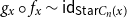 $g_x \circ f_x \sim\mathsf{id}_{\mathsf{Star}{C_n}(x)}$
by performing a case analysis on the second component of a term
$g_x \circ f_x \sim\mathsf{id}_{\mathsf{Star}{C_n}(x)}$
by performing a case analysis on the second component of a term
 $(y, z) : \mathsf{Star}_{C_n}(x)$
. Specifically, we consider whether z is either
$(y, z) : \mathsf{Star}_{C_n}(x)$
. Specifically, we consider whether z is either
 $\mathsf{inl}(u)$
or
$\mathsf{inl}(u)$
or
 $\mathsf{inr}(v)$
. For the first case, we need to prove that
$\mathsf{inr}(v)$
. For the first case, we need to prove that
 $g_x (f_x ((y, \mathsf{inl}(u)))) = (y,\mathsf{inl}(u))$
. Evaluating the expression of the composite, we obtain an equality with the question mark below, which we need to show one can inhabit:
$g_x (f_x ((y, \mathsf{inl}(u)))) = (y,\mathsf{inl}(u))$
. Evaluating the expression of the composite, we obtain an equality with the question mark below, which we need to show one can inhabit:
 \begin{equation*} \begin{split} &g_x (f_x ((y, \mathsf{inl}(u)))) \equiv g_x((0,!)) \equiv (\mathsf{suc}(x), \mathsf{inl}(a^{+})) \overset{?}{=} (y, \mathsf{inl}(u)). \end{split}\end{equation*}
However, we can establish the required equality by noting that
 ${{\mathsf{E}}}_{C_n}(x,\mathsf{suc}(x))$
is contractible. This implies that
${{\mathsf{E}}}_{C_n}(x,\mathsf{suc}(x))$
is contractible. This implies that
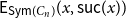 ${{\mathsf{E}}}_{\mathsf{Sym}(C_n)}(x, \mathsf{suc}(x))$
is a proposition, which in turn implies that
${{\mathsf{E}}}_{\mathsf{Sym}(C_n)}(x, \mathsf{suc}(x))$
is a proposition, which in turn implies that
 $a^{+} = u$
and that we have
$a^{+} = u$
and that we have
 $y = \mathsf{suc}(x)$
. Similarly, we can show that
$y = \mathsf{suc}(x)$
. Similarly, we can show that
 $g_x (f_x ((y, \mathsf{inr}(v)))) = (y, \mathsf{inr}(v))$
. This completes the proof that
$g_x (f_x ((y, \mathsf{inr}(v)))) = (y, \mathsf{inr}(v))$
. This completes the proof that
 $f_x$
is an equivalence and shows that
$f_x$
is an equivalence and shows that
 $\mathsf{Star}_{C_n}(x)$
has only two elements.
$\mathsf{Star}_{C_n}(x)$
has only two elements.
Theorem 4.6. If G is a (finite) graph, then the type
 $\mathsf{Star}_{G}(x)$
is a (finite) set.
$\mathsf{Star}_{G}(x)$
is a (finite) set.
Proof. The conclusion follows since the base type in Definition 4.4 is the set of edges in the graph, and each of the fibres of the
 $\Sigma$
-type is a set since they are coproducts of sets. In particular, if the graph is finite, then all the types appearing in the type
$\Sigma$
-type is a set since they are coproducts of sets. In particular, if the graph is finite, then all the types appearing in the type
 $\mathsf{Star}_{G}(x)$
are finite sets, and then our conclusion follows.
$\mathsf{Star}_{G}(x)$
are finite sets, and then our conclusion follows.
4.3 The type of graph maps
A combinatorial map is a specific type of data structure that is used to represent a graph that is embedded in a surface. This data structure offers a powerful substitute for traditional analytic/geometric techniques for representing such embeddings. Unlike geometric methods, combinatorial maps allow us to represent the combinatorial structure of the topological embedding without the need to explicitly work with the surface in which the graph is embedded.
In this work, we focus on defining the type of combinatorial maps in type theory; see Definition 4.7. We then turn our attention to a particular kind of embedding, cellular embeddings. The reason for this focus is that all graph maps in the two-dimensional plane are cellular embeddings. Therefore, drawing graphs in the plane without edge crossings can be represented by cellular embeddings.
Cellular embeddings are particularly interesting because they can be characterised combinatorially up to isotopy by the cyclic order they induce in the set of nodes around each node in the graph (Gross and Tucker Reference Gross and Tucker1987), as illustrated in Fig. 5(b). This characterisation is minimal, as no additional information is required beyond the cyclic orders.
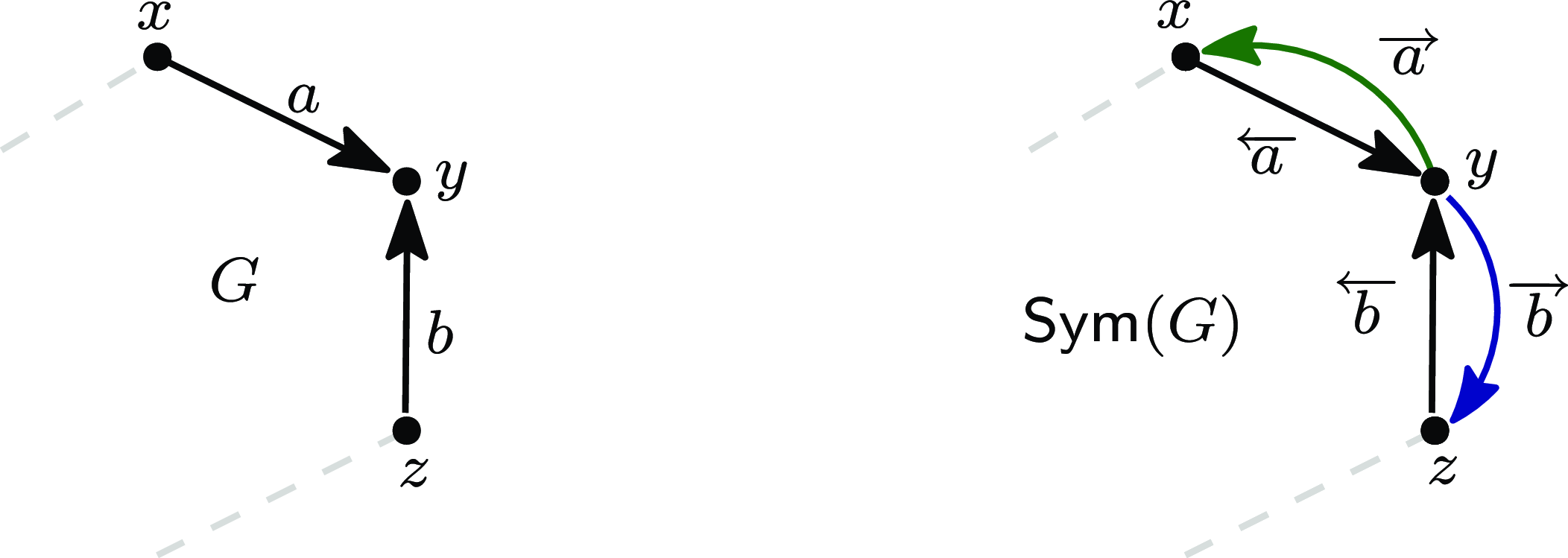
Figure 4. On the left we show a part of a graph G with two distinguished edges, a and b. On the right we show the corresponding symmetrisation,
 $\mathsf{Sym}(G)$
, including the two edges,
$\mathsf{Sym}(G)$
, including the two edges,
 $\overleftarrow{a}$
and
$\overleftarrow{a}$
and
 $\overrightarrow{a}$
induced by a, and similarly,
$\overrightarrow{a}$
induced by a, and similarly,
 $\overleftarrow{b}$
and
$\overleftarrow{b}$
and
 $\overrightarrow{b}$
induced by b. For brevity, we will only draw a segment representing related edges in the symmetrisation, as in Fig. 5(b).
$\overrightarrow{b}$
induced by b. For brevity, we will only draw a segment representing related edges in the symmetrisation, as in Fig. 5(b).

Figure 5. We show in (a) the drawing of a graph G with edge crossings. A representation of the graph G embedded in the sphere is shown in (b). The corresponding faces of the graph map shaded in (b) are named
 $F_i$
for i from 1 to 6. It is shown in (c) with fuchsia colour the incident edges at the node a in
$F_i$
for i from 1 to 6. It is shown in (c) with fuchsia colour the incident edges at the node a in
 $\mathsf{Sym}(G)$
. The rotation system at a, that is, the cyclic set denoted by
$\mathsf{Sym}(G)$
. The rotation system at a, that is, the cyclic set denoted by
 $(ba\,ad\,ax)$
, is shown in green colour. The dashed lines represent edges not visible to the view.
$(ba\,ad\,ax)$
, is shown in green colour. The dashed lines represent edges not visible to the view.
One observation is that not all finite graphs can be drawn in the plane, but all finite graphs can be drawn on some orientable surface (Stahl Reference Stahl1978). The literature in graph theory has proven that a graph cannot have a cellular embedding on any surface if it has at least one node of infinite valency (Mohar Reference Mohar1988, Proposition Section S3.2). As our focus is on cellular embeddings, we will only examine locally finite graphs throughout the document.
Definition 4.7.
 $\mathsf{Map}(G)$
is the type of combinatorial maps (maps for short) for a graph G defined as follows:
$\mathsf{Map}(G)$
is the type of combinatorial maps (maps for short) for a graph G defined as follows:
 \begin{align*} \mathsf{Map}(G) & :\equiv \prod_{(x\,:\,{{\mathsf{N}}}_{G})} \mathsf{Cyclic}(\mathsf{Star}_{G}(x)). \end{align*}
Definition 4.8. A graph G is locally finite if the set of incident edges at the star at any node x in G, is a finite set.
Theorem 4.9. If the type
 $\mathsf{Map}(G)$
is inhabited, then the graph G is locally finite.
$\mathsf{Map}(G)$
is inhabited, then the graph G is locally finite.
Proof. A map of G provides each node a cyclic order on its star. Since these orders are finite by Theorem 2.17, the local finiteness of G follows.
Theorem 4.10. The type of maps for a (finite) graph forms a (finite) set.
Proof. The type
 $\mathsf{Map}(G)$
is a set using the closure property of
$\mathsf{Map}(G)$
is a set using the closure property of
 $\Pi$
-types under (finite) sets. The type
$\Pi$
-types under (finite) sets. The type
 $\mathsf{Cyclic}(\mathsf{Star}_{G}(x))$
is a finite set by Theorem 2.17.
$\mathsf{Cyclic}(\mathsf{Star}_{G}(x))$
is a finite set by Theorem 2.17.
For brevity, we use from now the variable
 $\mathscr{M}$
to denote a map of the graph G.
$\mathscr{M}$
to denote a map of the graph G.
Example 4.11. The possible maps for the cycle
 $C_n$
for
$C_n$
for
 $n>0$
can be listed considering the cyclic structures of the two-point type. These correspond to the cyclic structures of the stars of
$n>0$
can be listed considering the cyclic structures of the two-point type. These correspond to the cyclic structures of the stars of
 $C_n$
, see the correspondence exhibited in Example 4.5. The two maps are given by the following functions:
$C_n$
, see the correspondence exhibited in Example 4.5. The two maps are given by the following functions:
-
⊳
$c_1 :\equiv \langle [\![ 2]\!], \mathsf{pred}, 2\rangle$
and -
•
$c_2 :\equiv \langle [\![ 2]\!], \mathsf{suc}, 2\rangle$
.
5. The Type of Faces
In the context of cellular embeddings, faces correspond to regions homeomorphic, to the open disk. Combinatorially, a face associated with a graph map consists of a cyclic walk in the embedded graph where no edges are inside the cycle, and no node occurs twice. Definition 5.3 is our attempt to make this intuition formal.
The first component of a face, as in Definition 5.3, captures the concept that its edges form a cyclic walk in the embedded graph. While working with such walks would typically necessitate a fixed starting point, this point does not contribute to the face’s combinatorial structure. Hence, we can employ a cyclic graph to represent all such cyclic walks, thereby obviating the need for any distinguished starting point in such walks.
The second component, the map-compatibility property, explicitly defines the ‘no edges on the inside’ criterion for a face. This criterion is captured by the fact that each pair of consecutive edges on the face is a successor-predecessor pair in the cyclic order of the edges around their common node. In other words, when we move along the edges of the face either clockwise or counterclockwise, we will never come across an edge that goes through the inside of the face. As our graphs are directed, we must traverse the edges in the symmetrisation of the graph rather than the graph itself.
The following two definitions are used in the definition of the type of faces.
Definition 5.1. A graph homomorphism h from G to H given by
 $(\alpha, \beta)$
is edge-injective, denoted by
$(\alpha, \beta)$
is edge-injective, denoted by
 $\mathsf{isEdgeInj}(h)$
, if the function f defined below is an embedding:
$\mathsf{isEdgeInj}(h)$
, if the function f defined below is an embedding:
 \begin{align*} & f : \sum_{(x,y~:~{{\mathsf{N}}}_{G})} {{\mathsf{E}}}_{G}(x,y) \to \sum_{(x,y~:~{{\mathsf{N}}}_{H})} {{\mathsf{E}}}_{H}(x,y). \\ & f~(x,y,e) :\equiv (\alpha(x), \alpha(y), \beta(x,y,e)). \end{align*}
Definition 5.2. The function
 $\mathsf{flip}$
changes the direction of an edge in
$\mathsf{flip}$
changes the direction of an edge in
 $\mathsf{Sym}(G)$
:
$\mathsf{Sym}(G)$
:
 \begin{equation*} \begin{split} &\mathsf{flip}\,:\prod_{(x,y\,:{{\mathsf{N}}}_{G})} {{\mathsf{E}}}_{\mathsf{Sym}(G)}(x,y)~\to~{{\mathsf{E}}}_{\mathsf{Sym}(G)}(y,x).\\ &\mathsf{flip}~(x,y,\mathsf{inl}(e))~:\equiv ~\mathsf{inr}(e).\\ &\mathsf{flip}~(x,y,\mathsf{inr}(e))~:\equiv ~\mathsf{inl}(e). \end{split} \end{equation*}
Since the first two arguments of the function
 $\mathsf{flip}$
are inferrable from the third argument, we will omit them below.
$\mathsf{flip}$
are inferrable from the third argument, we will omit them below.
Definition 5.3. The type
 $\mathsf{Face}(G, \mathscr{M})$
is the type of faces of a combinatorial map
$\mathsf{Face}(G, \mathscr{M})$
is the type of faces of a combinatorial map
 $\mathscr{M}$
of a graph G. A face of type
$\mathscr{M}$
of a graph G. A face of type
 $\mathsf{Face}(G, \mathscr{M})$
consists of:
$\mathsf{Face}(G, \mathscr{M})$
consists of:
-
(1) a cyclic graph A,
-
(2) a graph homomorphism h given by
$(\alpha, \beta)$
of type
${{\mathsf{Hom}({A},{\mathsf{Sym}(G)})}}$
, such that-
a. h is edge-injective,
-
b. h is map-compatible, denoted by
$\mathsf{isMapComp}(h)$
, meaning that h is star-compatible and corner-preserving, properties defined below, respectively.-
* h is star-compatible, if the condition in (13) holds for every
$x : {{\mathsf{N}}}_{A}$
, (13)
\begin{equation}\mathsf{isStarComp}(h)(x):\equiv \| \mathsf{Star}_{G}(\alpha(x)) \| \to \|\mathsf{Star}_{A}(x) \|. \end{equation}
-
* h is corner-compatible, if there is evidence that h is compatible with the edge-ordering given by the map
$\mathscr{M}$
at the node
$\alpha(x)$
and the edge-ordering coming from the star at that node x in A. To state this property, let us consider the following notation.-
* The previous edge at x is the edge
$a : {{\mathsf{E}}}_{{{\mathsf{N}}}_{A}}(\mathsf{pred}(x), x)$
, -
* the edge after
$a_x$
is the edge denoted by
$a_x^{+}$
of type
${{\mathsf{E}}}_{{{\mathsf{N}}}_{A}}(x , \mathsf{suc}(x))$
, as illustrated in Fig. 6, and -
* since
$\mathscr{M}(\alpha(x))$
is a triple like
$\langle f, m , ! \rangle$
of type for some function
$$\mathsf{Cyclic}(\mathsf{Star}_{G}(\alpha(x)))$$
$f : \mathsf{Star}_{G}(\alpha(x)) \to \mathsf{Star}_{G}(\alpha(x))$
and some number m (the cardinality of the star at
$\alpha(x)$
), we abuse notation and use
$\mathscr{M}(\alpha(x))$
to denote the function f. See more on the cyclic type in Definition 2.11: (14)
\begin{equation}\begin{split}\mathsf{isCornerComp}(h)(x) :\equiv & \mathscr{M}(\alpha(x))((\alpha (\mathsf{pred}(x)) , \mathsf{flip}(\beta(\mathsf{pred}(x),x,a))))\\ &=_{\mathsf{Star}_{G}(\alpha(x))} (\,\alpha(\mathsf{suc}(x))\,,\,\beta(x, \mathsf{suc}(x),a^{+})\,). \end{split} \end{equation}
-
-
-


Figure 6. On the right side, we shade the face F of the graph G embedded in the sphere given in Fig. 5. We have the cycle graph
 $C_3$
and
$C_3$
and
 $h:\mathsf{Hom}(C_3,\mathsf{Sym}(G))$
given by
$h:\mathsf{Hom}(C_3,\mathsf{Sym}(G))$
given by
 $(\alpha, \beta)$
on the left side.
$(\alpha, \beta)$
on the left side.
 $C_3$
and h can be used to define the face F using
$C_3$
and h can be used to define the face F using
 $C_3$
as the graph A in Definition 5.3.
$C_3$
as the graph A in Definition 5.3.
It should be noted that the truncation in (13) is intentional. By incorporating this, we aim to emphasise that if the graph G has at least one edge at a given node, then a face covering that node, represented by the cyclic graph A, must have at least one edge at the corresponding node as well. Without this condition, the type of faces could be inhabited with empty faces using A as the cyclic graph without edges (
 $C_0$
) at every node of the graph G. In Fig. 6, we illustrate a portion of the required data to define a face
$C_0$
) at every node of the graph G. In Fig. 6, we illustrate a portion of the required data to define a face
 $F_1$
for the map of graph G given in Fig. 5(b).
$F_1$
for the map of graph G given in Fig. 5(b).
Theorem 5.4. For a graph homomorphism, being edge-injective is a proposition.
Proof. Edge-injectivity is a proposition by iteratively applying the closure of
 $\Pi$
-types to propositions. Ultimately, we need to show that for any two terms
$\Pi$
-types to propositions. Ultimately, we need to show that for any two terms
 $(x , y , e_1)$
and
$(x , y , e_1)$
and
 $(x' , y' , e_2)$
in
$(x' , y' , e_2)$
in
 $\Sigma_{x,y~:~{{\mathsf{N}}}_{G}} {{\mathsf{E}}}_{G}(x,y)$
, the identity type
$\Sigma_{x,y~:~{{\mathsf{N}}}_{G}} {{\mathsf{E}}}_{G}(x,y)$
, the identity type
 $(x , y , e_1) = (x' , y' , e_2)$
is a proposition. This is true because the
$(x , y , e_1) = (x' , y' , e_2)$
is a proposition. This is true because the
 $\Sigma$
-type in question is a set, and sets are closed under
$\Sigma$
-type in question is a set, and sets are closed under
 $\Sigma$
-types, given that both
$\Sigma$
-types, given that both
 ${{\mathsf{N}}}_{G}$
and
${{\mathsf{N}}}_{G}$
and
 ${{\mathsf{E}}}_{G}(x,y)$
are sets.
${{\mathsf{E}}}_{G}(x,y)$
are sets.
Theorem 5.5. For a graph homomorphism, being map-compatible is a proposition.
Proof. For a graph homomorphism h, map-compatibility decomposes into star-compatibility and corner-compatibility. We must show each type in this product is a proposition. Star-compatibility is a proposition as it involves a function type with a propositional codomain – the propositional truncation of a set. Corner-compatibility is also a proposition, being a function type whose codomain is the identity type on
 $\mathsf{Star}_{G}(\alpha(x))$
at
$\mathsf{Star}_{G}(\alpha(x))$
at
 $\alpha(x)$
. This identity type is a proposition since stars are sets, as established in Theorem 4.6.
$\alpha(x)$
. This identity type is a proposition since stars are sets, as established in Theorem 4.6.
We devote the rest of this section to proving that the type of faces forms a set in Theorem 5.7. This claim rests on the fact that (i) the type of cyclic graphs forms a set, (ii) the type of graph homomorphisms forms a set, and (iii) the conditions, edge-injective and map-compatible in, Definition 5.3 are propositions. One might suspect that this type forms a groupoid based on previous facts. However, the edge-injectivity property of the underlying graph homomorphism of each face suffices to show that the type of faces is a set.
Theorem 5.6. Let f and g be edge-injective graph homomorphisms from
 $C_{n}$
to a graph G and
$C_{n}$
to a graph G and
 $n>0$
. Then the type
$n>0$
. Then the type
 $\Sigma_{e : C_{n} = C_{n}}~({{\mathsf{tr}^{\lambda X.{{\mathsf{Hom}({X},{G})}}}(e,f)}} = g)$
is a proposition.
$\Sigma_{e : C_{n} = C_{n}}~({{\mathsf{tr}^{\lambda X.{{\mathsf{Hom}({X},{G})}}}(e,f)}} = g)$
is a proposition.

Proof. The result follows from the proof that the
 $\Sigma$
-type in question is equivalent to a proposition. The corresponding equivalence is given in (15), in which we use some known results about Univalence and Theorem 3.19, as in the very last step:
$\Sigma$
-type in question is equivalent to a proposition. The corresponding equivalence is given in (15), in which we use some known results about Univalence and Theorem 3.19, as in the very last step:


It remains to show that the last equivalent type is a proposition. Let
 $(k_1 , p_1)$
and
$(k_1 , p_1)$
and
 $(k_2, p_2)$
be of type
$(k_2, p_2)$
be of type
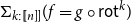 $\Sigma_{k : [\![ n]\!]} (f = g \circ \mathsf{rot}^{k})$
. We must show that
$\Sigma_{k : [\![ n]\!]} (f = g \circ \mathsf{rot}^{k})$
. We must show that
 $(k_1 , p_1)$
is equal to
$(k_1 , p_1)$
is equal to
 $(k_2, p_2)$
. Since
$(k_2, p_2)$
. Since
 ${{\mathsf{Hom}({C_n},{G})}}$
is a set, we only need to prove that
${{\mathsf{Hom}({C_n},{G})}}$
is a set, we only need to prove that
 $k_1$
is equal to
$k_1$
is equal to
 $k_2$
. To show that, Theorem 3.19 is used in the proof. By computing the identity type of graph isomorphisms, we obtain that
$k_2$
. To show that, Theorem 3.19 is used in the proof. By computing the identity type of graph isomorphisms, we obtain that
 $p_1^{-1} \cdot p_2$
of type
$p_1^{-1} \cdot p_2$
of type
 $g \circ \mathsf{rot}^{k_1} = g \circ \mathsf{rot}^{k_2}$
is equivalent to having two equalities:
$g \circ \mathsf{rot}^{k_1} = g \circ \mathsf{rot}^{k_2}$
is equivalent to having two equalities:
-
⊳
$p :\pi_1(g \circ \mathsf{rot}^{k_1}) = \pi_1(g \circ \mathsf{rot}^{k_2})$
and -
⊳
$q : {{\mathsf{tr}^{\lambda e.\prod_{x,y~:~{{\mathsf{N}}}_{C_n}} {{\mathsf{E}}}_{C_n}(x,y) \to {{\mathsf{E}}}_{G}(e(x),e(y)) }(, )}} {p}{\pi_2(g \circ \mathsf{rot}^{k_1})} = \pi_2(g \circ \mathsf{rot}^{k_2})$
.


By characterising the identity of the
 $\Sigma$
-types and with the previous equalities, p and q, one can get another equality r of the type in (16) for
$\Sigma$
-types and with the previous equalities, p and q, one can get another equality r of the type in (16) for
 $x,y:{{\mathsf{N}}}_{C_n}$
and
$x,y:{{\mathsf{N}}}_{C_n}$
and
 $e:{{\mathsf{E}}}_{C_n}(x,y)$
:
$e:{{\mathsf{E}}}_{C_n}(x,y)$
:
 \begin{equation}\begin{array}{lll} ( (\pi_1(g \circ \mathsf{rot}^{k_{i}}))(x) , & (\pi_1(g \circ \mathsf{rot}^{k_{i}}))(y) , & (\pi_2(g \circ \mathsf{rot}^{k_{i}}))(x,y,e) ) = \\ ( (((\pi_1(g))(\pi_1(\mathsf{rot}^{k_{i}}))) (x)) , & (((\pi_1(g))(\pi_1(\mathsf{rot}^{k_{i}}))) (y)) , & (((\pi_2(g))(\pi_2(\mathsf{rot}^{k_{i}}))) (x,y,e)) ). \end{array} \end{equation}
Now since the graph homomorphism g is edge-injective, applying Definition 5.1 to the equality r, one gets an equality r’ of the type below in (17). By applying Theorem 3.19 to r’, we conclude that
 $k_1$
is equal to
$k_1$
is equal to
 $k_2$
from which the required conclusion follows:
$k_2$
from which the required conclusion follows:
 \begin{equation} \begin{aligned}&( (\pi_1(\mathsf{rot}^{k_{1}}))(x) , (\pi_1(\mathsf{rot}^{k_{1}}))(y) , (\pi_2(\mathsf{rot}^{k_{1}}))(x,y,e))=\\ &( (\pi_1(\mathsf{rot}^{k_{2}}))(x) , (\pi_1(\mathsf{rot}^{k_{2}}))(y) , (\pi_2(\mathsf{rot}^{k_{2}}))(x,y,e)). \end{aligned} \end{equation}
Theorem 5.7. The type of faces for a graph map forms a set.
Proof. Let
 $F_1$
and
$F_1$
and
 $F_2$
be two faces of a map
$F_2$
be two faces of a map
 $\mathscr{M}$
. We will show that the type
$\mathscr{M}$
. We will show that the type
 $F_1 = F_2$
is a proposition in (18), with the following conventions.
$F_1 = F_2$
is a proposition in (18), with the following conventions.
-
⊳
$\mathscr{A}$
is the cyclic graph related to the face
$F_1$
:
\begin{equation*} \mathscr{A} :\equiv (A, (\varphi_{A}, n,\mathsf{isCyclic}(A,\varphi_{A},n))). \end{equation*}
-
⊳
$\mathscr{B}$
is the cyclic graph related to the face
$F_2$
:
\begin{equation*} \mathscr{B} :\equiv (B, (\varphi_{B}, m,\mathsf{isCyclic}(B,\varphi_{B},m))). \end{equation*}


We first unfold the definitions of
 $F_1$
and
$F_1$
and
 $F_2$
in (18a) and simplify the propositions in (18b), namely
$F_2$
in (18a) and simplify the propositions in (18b), namely
 $\mathsf{isEdgeInj}$
,
$\mathsf{isEdgeInj}$
,
 $\mathsf{isMapComp}$
and
$\mathsf{isMapComp}$
and
 $\mathsf{isCyclic}$
. Then, by expanding the definitions of
$\mathsf{isCyclic}$
. Then, by expanding the definitions of
 $\mathscr{A}$
and
$\mathscr{A}$
and
 $\mathscr{B}$
in (18c) and simplifying the propositions in terms such as being a cyclic graph, one gets (18d). Next, we reorder in (18d) the tuple equalities to create an opportunity for path induction towards the application of Theorem 5.6. Now, since we want to prove that the type of faces is a set, and that itself is a proposition, the truncation elimination principle is applied to the propositions
$\mathscr{B}$
in (18c) and simplifying the propositions in terms such as being a cyclic graph, one gets (18d). Next, we reorder in (18d) the tuple equalities to create an opportunity for path induction towards the application of Theorem 5.6. Now, since we want to prove that the type of faces is a set, and that itself is a proposition, the truncation elimination principle is applied to the propositions
 $\mathsf{isCyclic}(A,\varphi_{A},n)$
and
$\mathsf{isCyclic}(A,\varphi_{A},n)$
and
 $\mathsf{isCyclic}(A,\varphi_{A},n)$
. Then, the graphs A and B become, respectively,
$\mathsf{isCyclic}(A,\varphi_{A},n)$
. Then, the graphs A and B become, respectively,
 $C_n$
and
$C_n$
and
 $C_m$
in (18e). The step in (18f) follows from the characterisation of the identity type between tuples in a nested
$C_m$
in (18e). The step in (18f) follows from the characterisation of the identity type between tuples in a nested
 $\Sigma$
-type: calc]proof:face-is-set
$\Sigma$
-type: calc]proof:face-is-set


It only remains to show that the type in (18f) is a proposition. We show this by proving that each type in (18f) is a proposition. First, we unfold the cyclic graph definition for
 $C_n$
and
$C_n$
and
 $C_m$
, using Definition 3.18. Second, a case analysis on n and m is performed. This approach creates four cases where n and m can be zero or positive. However, we only keep the cases where n and m are structurally equal. One can show that the other cases are imposible with an equality between n and m.
$C_m$
, using Definition 3.18. Second, a case analysis on n and m is performed. This approach creates four cases where n and m can be zero or positive. However, we only keep the cases where n and m are structurally equal. One can show that the other cases are imposible with an equality between n and m.
-
1. If n and m are zero, then, by definition,
$C_n$
and
$C_m$
are the one-point graph. In this case, the conclusion follows easily. The base type
$n = m$
of the total space in (18f) is a proposition because
$\mathbb{N}$
is a set. The type
$C_0 = C_0$
is a proposition, since it is contractible. The identity graph homomorphism is the unique automorphism of
$C_0$
. Lastly, because
${{\mathsf{Hom}({C_n},{C_n})}}$
is a set, the remaining type of the
$\Sigma$
-type is a proposition, completing the proof obligations. -
2. If n and m are positive, we reason similarly. The type
$n = m$
is a proposition. By path induction on
$p : n = m$
, the second base type of the
$\Sigma$
-type becomes the type in (19): (19)which is a proposition by Theorem 5.6. The remaining type of the
\begin{equation}\sum_{(e~:~C_{n} = C_{n})} ({{\mathsf{tr}^{\lambda X .{{\mathsf{Hom}({X},{\mathsf{Sym}(G)})}}}(e,f)}} = g), \end{equation}
$\Sigma$
-type is a proposition, because
${{\mathsf{Hom}({C_n},{C_n})}}$
is a set. Therefore, the
$\Sigma$
-type in (18f) is a proposition as required.


5.1 The boundary of a face
Each face
 $\mathscr{F}$
of a map
$\mathscr{F}$
of a map
 $\mathscr{M}$
consisting of a cyclic graph A, a homomorphism h and some extra data as described in Definition 5.3 induced a closed walk that follows the edges of its defining polygon, which we refer to as its boundary.
$\mathscr{M}$
consisting of a cyclic graph A, a homomorphism h and some extra data as described in Definition 5.3 induced a closed walk that follows the edges of its defining polygon, which we refer to as its boundary.
Definition 5.8. Let
 $\mathscr{F}$
be a face for a map of the graph G, the boundary of
$\mathscr{F}$
be a face for a map of the graph G, the boundary of
 $\partial \mathscr{F}$
is the subgraph of the image of the associated function, h, given in the definition of the type of
$\partial \mathscr{F}$
is the subgraph of the image of the associated function, h, given in the definition of the type of
 $\mathscr{F}$
:
$\mathscr{F}$
:
 \begin{equation*} \partial \mathscr{F} \equiv \partial ((A, (h, -))) :\equiv \mathsf{Img}(h). \end{equation*}
Here,
 $\mathsf{Img}(h)$
is the induced subgraph of G by the image of h. More specifically, it is defined as:
$\mathsf{Img}(h)$
is the induced subgraph of G by the image of h. More specifically, it is defined as:
 \begin{equation*} \mathsf{Img}(h) :\equiv (\Sigma_{x:{{\mathsf{N}}}_{A}},\pi_1(h)(x), \lambda x.\lambda y.\lambda e. \pi_2(h)(x,y,e)). \end{equation*}
The degree of a face
 $\mathscr{F}$
is the length of
$\mathscr{F}$
is the length of
 $\partial \mathscr{F}$
, which is the number of nodes in A. The boundary
$\partial \mathscr{F}$
, which is the number of nodes in A. The boundary
 $\partial \mathscr{F}$
can be walked in two directions with respect to the orientation given by its map.
$\partial \mathscr{F}$
can be walked in two directions with respect to the orientation given by its map.
As illustrated by Fig. 7, given two different nodes x and y in
 $\partial \mathscr{F}$
, we can connect x to y using the walk in the clockwise direction,
$\partial \mathscr{F}$
, we can connect x to y using the walk in the clockwise direction,
 $\mathsf{cw}_{\mathscr{F}}(x,y)$
. Similarly, one can connect x to y using the walk in the counterclockwise direction,
$\mathsf{cw}_{\mathscr{F}}(x,y)$
. Similarly, one can connect x to y using the walk in the counterclockwise direction,
 $\mathsf{ccw}_{\mathscr{F}}(x,y)$
. Such walks are induced by the walks in the cyclic graph A, see Theorem 5.10.
$\mathsf{ccw}_{\mathscr{F}}(x,y)$
. Such walks are induced by the walks in the cyclic graph A, see Theorem 5.10.
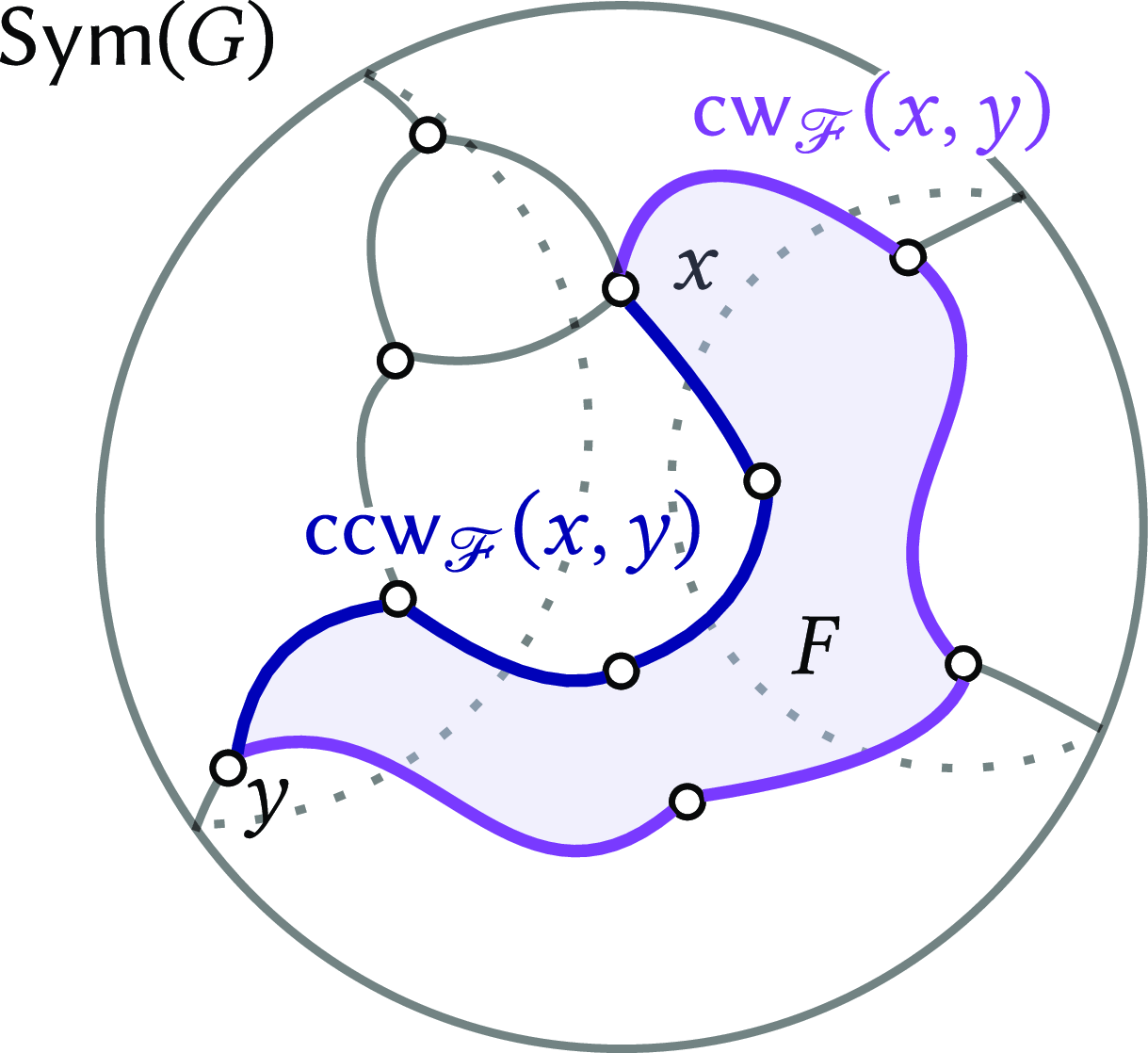
Figure 7. The graph embedding
 $\mathsf{Sym}(G)$
, as depicted in Fig. 5, is associated with a face
$\mathsf{Sym}(G)$
, as depicted in Fig. 5, is associated with a face
 $\mathscr{F}$
defined by
$\mathscr{F}$
defined by
 $\langle A , f\rangle$
. The underlying cyclic graph A contains two highlighted walks between distinct nodes x and y. These walks correspond to clockwise and counterclockwise closed walks in
$\langle A , f\rangle$
. The underlying cyclic graph A contains two highlighted walks between distinct nodes x and y. These walks correspond to clockwise and counterclockwise closed walks in
 $\mathsf{Sym}(G)$
, represented as
$\mathsf{Sym}(G)$
, represented as
 $\mathsf{cw}_{\mathscr{F}}(x,y)$
and
$\mathsf{cw}_{\mathscr{F}}(x,y)$
and
 $\mathsf{ccw}_{\mathscr{F}}(x,y)$
, respectively.
$\mathsf{ccw}_{\mathscr{F}}(x,y)$
, respectively.
For brevity, we omit the proofs of Theorems 5.9 and 5.10. These lemmas refer to properties inherent in the construction of
 $C_n$
and its symmetrisation, see Fig. 4. Thus, the proofs are straightforward applications of definitions.
$C_n$
and its symmetrisation, see Fig. 4. Thus, the proofs are straightforward applications of definitions.
Theorem 5.9. Supposing
 $x,y:{{\mathsf{N}}}_{C_{n}}$
, the following claims hold for the cycle graph
$x,y:{{\mathsf{N}}}_{C_{n}}$
, the following claims hold for the cycle graph
 $C_{n}$
.
$C_{n}$
.
-
(1) The type
${{\mathsf{E}}}_{C_{n}}(x,y)$
is a proposition. -
(2) For
$n>0$
, there exists an edge of type
${{\mathsf{E}}}_{C_{n}}(\mathsf{pred}(x), x)$
and an edge of type
${{\mathsf{E}}}_{C_{n}}(x, \mathsf{suc}(x))$
. -
(3) For
$n>0$
, there exists a walk going in the clockwise direction denoted by
$\mathsf{cw}_{C_n}(x,y)$
from x to y.


Theorem 5.10. Supposing
 $x,y:{{\mathsf{N}}}_{C_{n}}$
, the following claims hold for the graph
$x,y:{{\mathsf{N}}}_{C_{n}}$
, the following claims hold for the graph
 $\mathsf{Sym}(C_n)$
.
$\mathsf{Sym}(C_n)$
.
-
(1) If
$n > 1$
, then the type
${{\mathsf{E}}}_{\mathsf{Sym}(C_{n})}(x,y)$
is a proposition. -
(2) There exists an edge of type
${{\mathsf{E}}}_{\mathsf{Sym}(C_{n})}(\mathsf{pred}(x), x)$
and of type
${{\mathsf{E}}}_{\mathsf{Sym}(C_{n})}(x, \mathsf{suc}(x))$
. -
(3) There exist two walks from x to y in
$\mathsf{Sym}(C_{n})$
, denoted by
$\mathsf{cw}_{\mathsf{Sym}(C_{n})}(x,y)$
and
$\mathsf{ccw}_{\mathsf{Sym}(C_{n})}(x,y)$
, respectively.-
a. The walk
$\mathsf{cw}_{\mathsf{Sym}(C_{n})}(x,y)$
represents the walk in the clockwise direction from x to y. -
b. On the other hand, the walk
$\mathsf{ccw}_{\mathsf{Sym}(C_{n})}(x,y)$
represents the walk in the counterclockwise direction from x to y. In case
$x = y$
, the walk
$\mathsf{ccw}_{\mathsf{Sym}(C_{n})}(x,y)$
corresponds to the trivial walk
$\langle x \rangle$
.
-


Example 5.11. For cycle graphs
 $C_n$
, only one combinatorial map exists. Cyclic structures of two-point type
$C_n$
, only one combinatorial map exists. Cyclic structures of two-point type
 $c_1$
and
$c_1$
and
 $c_2$
, defined in Example 4.5, precisely induce the maps of
$c_2$
, defined in Example 4.5, precisely induce the maps of
 $C_n$
. In other words, one can obtain a map
$C_n$
. In other words, one can obtain a map
 $\mathscr{M}$
using
$\mathscr{M}$
using
 $c_1$
by (20) and
$c_1$
by (20) and
 \begin{equation*} (\mathsf{pred}, 2, |(\mathsf{ideqv}, \mathsf{refl}_{\mathsf{pred}}) |) : \mathsf{Cyclic}([\![ 2]\!]).\end{equation*}
Moreover, using function extensionality, Theorem 2.16 implies that the map induced by
 $c_2$
and the map
$c_2$
and the map
 $\mathscr{M}$
are equal.
$\mathscr{M}$
are equal.

Example 5.12. Recall that a graph consisting of a single node and n loop edges is referred to as an n-bouquet, denoted by
 $B_n$
. To enumerate the maps of
$B_n$
. To enumerate the maps of
 $B_2$
, we can label the edges of its sole star as (
$B_2$
, we can label the edges of its sole star as (
 $\overrightarrow{x}$
,
$\overrightarrow{x}$
,
 $\overleftarrow{x}$
,
$\overleftarrow{x}$
,
 $\overrightarrow{y}$
, and
$\overrightarrow{y}$
, and
 $\overleftarrow{y}$
). It is important to note that reflection is not treated as symmetry here. Consequently, we identify six distinct combinatorial maps for
$\overleftarrow{y}$
). It is important to note that reflection is not treated as symmetry here. Consequently, we identify six distinct combinatorial maps for
 $B_2$
, each distinct cyclic permutation of the set of edges creates a map in this case, as depicted in Fig. 8.
$B_2$
, each distinct cyclic permutation of the set of edges creates a map in this case, as depicted in Fig. 8.

Figure 8. The six possible maps of the bouquet
 $B_2$
. Respectively, they are denoted and defined as follows:
$B_2$
. Respectively, they are denoted and defined as follows:
 $a :\equiv (\overrightarrow{x},\overleftarrow{x}, \overrightarrow{y}, \overleftarrow{y})$
,
$a :\equiv (\overrightarrow{x},\overleftarrow{x}, \overrightarrow{y}, \overleftarrow{y})$
,
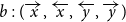 $b : (\overrightarrow{x},\overleftarrow{x}, \overleftarrow{y}, \overrightarrow{y})$
,
$b : (\overrightarrow{x},\overleftarrow{x}, \overleftarrow{y}, \overrightarrow{y})$
,
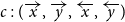 $c : (\overrightarrow{x}, \overrightarrow{y},\overleftarrow{x}, \overleftarrow{y})$
,
$c : (\overrightarrow{x}, \overrightarrow{y},\overleftarrow{x}, \overleftarrow{y})$
,
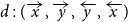 $d : (\overrightarrow{x}, \overrightarrow{y}, \overleftarrow{y},\overleftarrow{x})$
,
$d : (\overrightarrow{x}, \overrightarrow{y}, \overleftarrow{y},\overleftarrow{x})$
,
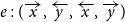 $e : (\overrightarrow{x}, \overleftarrow{y},\overleftarrow{x}, \overrightarrow{y})$
and
$e : (\overrightarrow{x}, \overleftarrow{y},\overleftarrow{x}, \overrightarrow{y})$
and
 $f :(\overrightarrow{x}, \overleftarrow{y}, \overrightarrow{y},\overleftarrow{x})$
.
$f :(\overrightarrow{x}, \overleftarrow{y}, \overrightarrow{y},\overleftarrow{x})$
.
6. Planar Maps
In this section, we examine the type of graphs with an embedding in the two-dimensional plane. Such embeddings are called planar embeddings or planar maps. A graph is planar if it has a planar map and the graph embedded is called a plane graph. To discuss the notion of planar embeddings, we take inspiration from topological graph theory (Gross and Tucker Reference Gross and Tucker1987, Section 3). Then one can work with combinatorial maps that represent graph maps into a surface – up to isotopy. In the following, we focus on describing embeddings of graphs in the sphere called spherical maps. These graph maps are used later to establish the type of planar embeddings for a given graph.
6.1 Spherical maps and homotopy for walks
Any graph map gives rise to an implicit surface. For planar embeddings, this surface is a space homeomorphic to the sphere. In particular, any embedding in the sphere induces an embedding in the plane. To see this, for a graph embedded in the sphere, one can puncture the sphere at some distinguished point, and subsequently, apply the stereographic projection to it.
The sphere in topology has two main invariants: path-connectedness and simply-connectedness. The former states that a path connects any pair of points in the sphere, and the latter states that any two paths with the same endpoints in the sphere can be deformed into one another.
If we now consider a walk as a path in the corresponding space induced by the map, then the path-connectedness property coincides with being connected for the graph embedded. However, if we want to address simply connectedness for the surface induced by a graph embedding, then we need to have an equivalent notion to saying how a pair of walks can be deformed into one the other. One proposal of such a notion is homotopy for walks in directed multigraphs (Prieto-Cubides 2022b).
In this subsection, we present a binary relation, denoted by
 $(\sim_{\mathscr{M}}\!)$
, on the set of walks between fixed endpoints in a graph as in introduced in Prieto-Cubides (2022b). This relation is designed to capture the behaviour of walks in an embedded graph in a surface such as the two-dimensional plane, where all the walks can be deformed one into another along the faces of the graph map in use.
$(\sim_{\mathscr{M}}\!)$
, on the set of walks between fixed endpoints in a graph as in introduced in Prieto-Cubides (2022b). This relation is designed to capture the behaviour of walks in an embedded graph in a surface such as the two-dimensional plane, where all the walks can be deformed one into another along the faces of the graph map in use.
Definition 6.1. Let
 $w_1,w_2$
be two walks from x to y in
$w_1,w_2$
be two walks from x to y in
 $\mathsf{Sym}(G)$
. The expression
$\mathsf{Sym}(G)$
. The expression
 ${{w_1\sim_{\mathscr{M}}w_2}}$
denotes that one can deform
${{w_1\sim_{\mathscr{M}}w_2}}$
denotes that one can deform
 $w_1$
into
$w_1$
into
 $w_2$
along the faces of
$w_2$
along the faces of
 $\mathscr{M}$
. We acknowledge evidence of this deformation as a walk homotopy between
$\mathscr{M}$
. We acknowledge evidence of this deformation as a walk homotopy between
 $w_1$
and
$w_1$
and
 $w_2$
, of type
$w_2$
, of type
 ${{w_1\sim_{\mathscr{M}}w_2}}$
.
${{w_1\sim_{\mathscr{M}}w_2}}$
.
The relation
 $(\sim_{\mathscr{M}}\!)$
has four constructors, as follows. The first three constructors are functions to indicate that homotopy for walks is an equivalence relation; they are
$(\sim_{\mathscr{M}}\!)$
has four constructors, as follows. The first three constructors are functions to indicate that homotopy for walks is an equivalence relation; they are
 $\mathsf{hrefl}$
,
$\mathsf{hrefl}$
,
 $\mathsf{hsym}$
and
$\mathsf{hsym}$
and
 $\mathsf{htrans}$
. Let
$\mathsf{htrans}$
. Let
 $x,y : {{\mathsf{N}}}_{G}$
.
$x,y : {{\mathsf{N}}}_{G}$
.
 \begin{equation} \begin{split} \mathsf{hrefl} &: \prod_{(w_1 : \mathsf{W}_{\mathsf{Sym}(G)}(x,y))}\,w_1 \sim_{\mathscr{M}} w_1.\\ \mathsf{hsym} &: \prod_{(w_1 , w_2 : \mathsf{W}_{\mathsf{Sym}(G)}(x,y))}\,w_1 \sim_{\mathscr{M}} w_2 \to w_2 \sim_{\mathscr{M}} w_1.\\ \mathsf{htrans} &: \prod_{(w_1 , w_2, w_3 : \mathsf{W}_{\mathsf{Sym}(G)}(x,y))}\,w_1 \sim_{\mathscr{M}} w_2 \to w_2 \sim_{\mathscr{M}} w_3 \to w_1 \sim_{\mathscr{M}} w_3. \end{split}\end{equation}
The fourth constructor, illustrated in Fig. 9, is the
 $\mathsf{hcollapse}$
function that establishes the walk homotopy:
$\mathsf{hcollapse}$
function that establishes the walk homotopy:
 \begin{equation*}{{(w_1 \cdot \mathsf{ccw}_{\mathscr{F}}(a,b) \cdot w_2)\sim_{\mathscr{M}} }}{(w_1 \cdot \mathsf{cw}_{\mathscr{F}}(a,b) \cdot w_2)},\end{equation*}
supposing one has the following,
-
(i) a face
$\mathscr{F}$
given by
$\langle A, f \rangle$
of the map
$\mathscr{M}$
, -
(ii) a walk
$w_1$
of type
$\mathsf{W}_{\mathsf{Sym}(G)}(x,f(a))$
for a node x in G with a node a in A, and -
(iii) a walk
$w_2$
of type
$\mathsf{W}_{\mathsf{Sym}(G)}(f(b),y)$
for a node b in A with a node y in G.


Figure 9. Given a face
 $\mathscr{F}$
of a map
$\mathscr{F}$
of a map
 $\mathscr{M}$
, we illustrate here
$\mathscr{M}$
, we illustrate here
 $\mathsf{hcollapse}$
, one of the four constructors of the homotopy relation on walks in Definition 6.1. The arrow
$\mathsf{hcollapse}$
, one of the four constructors of the homotopy relation on walks in Definition 6.1. The arrow
 $(\Downarrow)$
represents a homotopy of walks.
$(\Downarrow)$
represents a homotopy of walks.
One consequence of Definition 6.1 is that, in each face
 $\mathscr{F}$
, there is a walk homotopy between
$\mathscr{F}$
, there is a walk homotopy between
 $\mathsf{ccw}_{\mathscr{F}}(x,y)$
and
$\mathsf{ccw}_{\mathscr{F}}(x,y)$
and
 $\mathsf{cw}_{\mathscr{F}}(x,y)$
using the constructor
$\mathsf{cw}_{\mathscr{F}}(x,y)$
using the constructor
 $\mathsf{hcollapse}$
.
$\mathsf{hcollapse}$
.
The following shows how to compose walk homotopies horizontally and vertically. We consider a map
 $\mathscr{M}$
for a graph G and distinguishable nodes, x,y, and z where w,
$\mathscr{M}$
for a graph G and distinguishable nodes, x,y, and z where w,
 $w_1$
and
$w_1$
and
 $w_2$
are walks from x to y.
$w_2$
are walks from x to y.
Theorem 6.2. The following claims hold for the homotopy relation on walks.
-
(1) (Right whiskering) Let
$w_3$
be a walk of type
$\mathsf{W}_{\mathsf{Sym}(G)}(y,z)$
. If
${{w_1\sim_{\mathscr{M}}w_2}}$
then
${{(w_1 \cdot w_3)\sim_{\mathscr{M}}(w_2 \cdot w_3)}}$
.


-
(2) (Left whiskering) Let
$p_1,p_2$
be walks of type
$\mathsf{W}_{\mathsf{Sym}(G)}(y,z)$
. If
${{p_1\sim_{\mathscr{M}}p_2}}$
, then
${{(w \cdot p_1)\sim_{\mathscr{M}}(w \cdot p_2)}}$
.


-
(3) (Horizontal composition) Let
$p_1,p_2$
be walks of type
$\mathsf{W}_{\mathsf{Sym}(G)}(y,z)$
. If
${{w_1\sim_{\mathscr{M}}w_2}}$
and
${{p_1\sim_{\mathscr{M}}p_2}}$
, then
${{(w_1 \cdot p_1)\sim_{\mathscr{M}}(w_2 \cdot p_2)}}$
.


6.2 The type of spherical maps
In topology, the property of being simply connected to the sphere states that one can freely deform/contract any walk on the sphere into another whenever they share the same endpoints. This property of the sphere leads to the predicate in Definition 6.3, which sets the criteria for a graph to be embeddable in the 2-sphere.
Definition 6.3. Given a graph G, a map
 $\mathscr{M}$
for G is said to be spherical if the type in (22) is inhabited:
$\mathscr{M}$
for G is said to be spherical if the type in (22) is inhabited:
 \begin{equation}\mathsf{isSpherical}(\mathscr{M}):\equiv \prod_{(x,y : {{\mathsf{N}}}_{\mathsf{Sym}(G)})} \prod_{(w_1, w_2 : \mathsf{W}_{\mathsf{Sym}(G)}(x,y))}\parallel{{w_1\sim_{\mathscr{M}}w_2}} \parallel.\end{equation}
Theorem 6.4. Being spherical for a map is a proposition.
Proof. Since the codomain of the function type in (22) is a propositional truncation of a set of walk homotopies, it follows that it is indeed a proposition.
Theorem 6.5. The collection of all spherical maps for a graph forms a set.
Proof. Spherical maps constitute a subtype within the set of all graph maps by Theorem 6.4, thus forming a set.
Remark 1. When examining the definition of spherical maps in Definition 6.3, it becomes clear that showing that a map is spherical is not a simple task. To label a map as spherical, as per (22), one must evaluate all potential walk pairs for every node pair. This task can be daunting unless the set of walks exhibits a particular property. As a result, we suggest an alternative formulation for spherical maps based on a loop reduction procedure within a graph with a discrete node set.
Specifically, employing walk homotopies within a graph with a discrete node set and a pre-existing spherical map allows the reduction of any walk to an inner loop-free form, termed the normal form of a walk. The idea stems from the redundancy of loops, or the potential to simplify a loop into a point. Eradicating these loops results in a more tractable, yet equivalent, definition for spherical maps based on a loop reduction procedure for walks. Each walk is walk-homotopic to its normal form. It is also worth noting that one can determine if a map is spherical for graphs with a discrete node set. Additionally, the number of spherical maps for a graph is finite. For these results and their proofs, which exceed the scope of this text, we refer the reader to Prieto-Cubides (2022b).
6.3 The type of planar maps
Our goal is to characterise graph planarity within the framework of HoTT, guided by the intuitive idea that edges on a plane should not intersect. Defining the concept of edge intersection with precision poses a significant challenge. If we align with the geometric essence of this intuitive description, using the two-dimensional plane as our basis, it requires the use of real numbers (Univalent Foundations Program 2013, Section 10). This implies defining edge intersections in terms of points on the
 $\mathbb{R}^2$
plane and considering edges as curves within it. However, given its complexity, we opt for a combinatorial approach instead. As previously discussed, this method enables us to represent graph maps on the plane or, equivalently, a punctured 2-sphere, without any mention of real numbers.
$\mathbb{R}^2$
plane and considering edges as curves within it. However, given its complexity, we opt for a combinatorial approach instead. As previously discussed, this method enables us to represent graph maps on the plane or, equivalently, a punctured 2-sphere, without any mention of real numbers.
Definition 6.6. A connected and locally finite graph G is planar if the type
 $\mathsf{Planar}(G)$
is inhabited. Elements of
$\mathsf{Planar}(G)$
is inhabited. Elements of
 $\mathsf{Planar}(G)$
are called planar maps of G:
$\mathsf{Planar}(G)$
are called planar maps of G:
 \begin{equation*} \mathsf{Planar}(G) :\equiv \sum_{(\mathscr{M}~:~\mathsf{Map}(G))} \mathsf{isSpherical}(\mathscr{M}) \times \underbrace{{{\mathsf{Face}({G,\mathscr{M}}\!)}}}_{\mathrm{outer face}}.\end{equation*}
We define the type
 $\mathsf{Planar}(G)$
to represent all possible embeddings of G into the plane, specifically focusing on plane graphs. Although
$\mathsf{Planar}(G)$
to represent all possible embeddings of G into the plane, specifically focusing on plane graphs. Although
 $\mathsf{Planar}(G)$
is not a planarity test in itself, it can be used to determine if a finite graph is planar or not by generating all the maps of the graph and subsequently verifying their spherical nature and the presence of an outer face, see Theorem 6.4.
$\mathsf{Planar}(G)$
is not a planarity test in itself, it can be used to determine if a finite graph is planar or not by generating all the maps of the graph and subsequently verifying their spherical nature and the presence of an outer face, see Theorem 6.4.
Theorem 6.7. The type of all planar maps of a graph forms a set.
Proof. The type of planar maps in Definition 6.6 is not a proposition. It encompasses two sets: the set of combinatorial maps, see Theorem 4.10, and the set of faces, see Theorem 5.7. Since being spherical for a map is a mere proposition, one concludes that the
 $\Sigma$
-type collecting all planar maps of a graph forms a set.
$\Sigma$
-type collecting all planar maps of a graph forms a set.
In addition to their simple structure, cyclic graphs, and in particular
 $C_n$
graphs, are building blocks in a few relevant constructions in formal systems related to the study of the planarity of graphs, such as planar triangulations and the characterisation of all 2-connected planar graphs.
$C_n$
graphs, are building blocks in a few relevant constructions in formal systems related to the study of the planarity of graphs, such as planar triangulations and the characterisation of all 2-connected planar graphs.
Example 6.8. To show the planarity of
 $C_n$
, we begin with the base case
$C_n$
, we begin with the base case
 $n=0$
. The graph
$n=0$
. The graph
 $C_0$
is a unit graph, a graph with a single node
$C_0$
is a unit graph, a graph with a single node
 $\star$
and no edges. Without edges, the type of functions mapping this node to any cyclic order of its star is a contractible type, yielding a unique, trivially spherical map. The map is spherical since the only walk to consider is the empty walk, which is trivially homotopic to itself. Planarity follows as
$\star$
and no edges. Without edges, the type of functions mapping this node to any cyclic order of its star is a contractible type, yielding a unique, trivially spherical map. The map is spherical since the only walk to consider is the empty walk, which is trivially homotopic to itself. Planarity follows as
 $C_0$
is connected by definition and possesses an outer face. To define this face, we use as the base cyclic graph, the graph
$C_0$
is connected by definition and possesses an outer face. To define this face, we use as the base cyclic graph, the graph
 $C_0$
itself along with identity graph homomorphism h, see that
$C_0$
itself along with identity graph homomorphism h, see that
 $\mathsf{Sym}(C_0) \cong C_0$
. The other conditions to inhabit the type of faces for our map are thus trivially satisfied.
$\mathsf{Sym}(C_0) \cong C_0$
. The other conditions to inhabit the type of faces for our map are thus trivially satisfied.
For
 $n>0$
,
$n>0$
,
 $C_n$
is connected and locally finite as shown by Theorem 5.9. Its planarity is supported by Example 5.11, which confirms the existence of a unique map
$C_n$
is connected and locally finite as shown by Theorem 5.9. Its planarity is supported by Example 5.11, which confirms the existence of a unique map
 $\mathscr{M}$
for
$\mathscr{M}$
for
 $C_n$
. To show this map is spherical, it suffices to show that any two walks
$C_n$
. To show this map is spherical, it suffices to show that any two walks
 $w_1$
and
$w_1$
and
 $w_2$
with identical endpoints are homotopic. Inner loops in walks can be ignored since they are irrelevant to walk homotopy, as shown in Prieto-Cubides (2022b). Let us now consider the following cases. For
$w_2$
with identical endpoints are homotopic. Inner loops in walks can be ignored since they are irrelevant to walk homotopy, as shown in Prieto-Cubides (2022b). Let us now consider the following cases. For
 $n=1$
, the only walk is the trivial one, which is self-homotopic. For
$n=1$
, the only walk is the trivial one, which is self-homotopic. For
 $n>1$
, when examining nodes x and y in
$n>1$
, when examining nodes x and y in
 $C_n$
, we have:
$C_n$
, we have:
-
⊳ If
$x\neq y$
, the relevant walks are
$\mathsf{ccw}_{\mathsf{Sym}(C_{n})}(x,y)$
and
$\mathsf{cw}_{\mathsf{Sym}(C_{n})}(x,y)$
, as per Theorem 5.10. These walks are homotopic via
$\mathsf{hcollapse}(\mathscr{F}, x, y, x, y, \langle x \rangle, \langle y \rangle),$
where
$\mathscr{F}$
denotes the face associated with
$\mathsf{Sym}(C_{n})$
where these walks form the boundary of
$\mathscr{F}$
. -
• If
$x = y$
, the walks under consideration are the trivial walk at x and
$\mathsf{cw}_{\mathsf{Sym}(C_{n})}(x,x)$
. Similarly to the previous case, these walks are homotopic via
$\mathsf{hcollapse}$
.


Finally, the outer face of
 $\mathscr{M}$
is naturally induced by
$\mathscr{M}$
is naturally induced by
 $C_n$
, which satisfies Definition 5.3 by construction. In fact, the definition of faces in Definition 5.3 was informed by the structure of
$C_n$
, which satisfies Definition 5.3 by construction. In fact, the definition of faces in Definition 5.3 was informed by the structure of
 $C_n$
. Hence, we conclude that
$C_n$
. Hence, we conclude that
 $C_n$
is planar for all n.
$C_n$
is planar for all n.
In order to expand our collection of planar map examples, we will now explore the concept of planar extensions in the context of graph maps. This approach will provide a deeper understanding and additional instances of planar structures in graph theory.
6.4 Planar extensions
This subsection outlines the construction of planar maps from existing ones using the path addition operation. The inspiration for this construction derives from ear decompositions (Bang-Jensen and Gutin Reference Bang-Jensen and Gutin2009, Section 5.3), reliable networks, extensions of planar graphs for undirected graphs (Gross et al. Reference Gross, Yellen and Anderson2018, Section 5.2,7.3) and the characterisation of 2-connected graphs (Whitney Reference Whitney1932).
Definition 6.9. Let G be a graph with nodes u, v and
 $P_n$
denote a path graph of n nodes as defined in Definition 3.13. The (simple) path addition of
$P_n$
denote a path graph of n nodes as defined in Definition 3.13. The (simple) path addition of
 $P_n$
to G at nodes u and v in G is a new graph constructed using the function
$P_n$
to G at nodes u and v in G is a new graph constructed using the function
 $\mathsf{path\mbox{-}addition}$
with arguments
$\mathsf{path\mbox{-}addition}$
with arguments
 $G, u, v, n$
and r showing that n is positive, as illustrated in Fig. 13(a). For short, this new graph is denoted by
$G, u, v, n$
and r showing that n is positive, as illustrated in Fig. 13(a). For short, this new graph is denoted by
 $G \bullet_{u,v} P_n$
. Here, u and v are referred to as the endpoints of the addition:
$G \bullet_{u,v} P_n$
. Here, u and v are referred to as the endpoints of the addition:
 \begin{align*} &\mathsf{path\mbox{-}addition} : \prod_{(G : {{\mathsf{Graph}}}{})}\,\prod_{(u,\,v : {{\mathsf{N}}}_{G})}\,\prod_{(n : \mathbb{N})}\,(0 < n) \to {{\mathsf{Graph}}}{}.\\ &\mathsf{path\mbox{-}addition}\,(G, u, v, n, r) :\equiv (N', E', h_1, h_2). \end{align*}
The types of nodes N’ and the family of edges E’ are defined below. The functions
 $h_1$
and
$h_1$
and
 $h_2$
are well defined, although not elaborated here, see Prieto-Cubides (2022a) for details on these functions, their properties and other functions related to path additions:
$h_2$
are well defined, although not elaborated here, see Prieto-Cubides (2022a) for details on these functions, their properties and other functions related to path additions:
 \begin{align*} &N' :\equiv {{\mathsf{N}}}_{G} + [\![ n ]\!]. \\ &E' : N' \to N' \to \mathscr{U}. \\ &E'(\mathsf{inl}(x) , \mathsf{inl}(y))\,:\equiv {{\mathsf{E}}}_{G}(x,y). \\ &E'(\mathsf{inl}(x) , \mathsf{inr}(y))\,:\equiv (x = u) \times (y = (0 , r)). \\ &E'(\mathsf{inr}(x) , \mathsf{inl}(y))\,:\equiv (x = \mathsf{pred}((0 , r))) \times (y = v). \\ &E'(\mathsf{inr}(x) , \mathsf{inr}(y))\,:\equiv {{\mathsf{E}}}_{P_{n}}(x,y). \end{align*}
Remember that the path graph
 $P_n$
with n nodes can be defined as follows:
$P_n$
with n nodes can be defined as follows:
 \begin{equation*} P_n :\equiv ([\![ n ]\!], \lambda\,u\,v. \mathsf{toNat}(u) + 1 = \mathsf{toNat}(v)), \end{equation*}
where
 $\mathsf{toNat}$
is defined as follows:
$\mathsf{toNat}$
is defined as follows:
 \begin{equation*} \begin{array}[ht]{ll} & \mathsf{toNat} : [\![ n ]\!] \to \mathbb{N}. \\ & \mathsf{toNat}(k, !) :\equiv k. \end{array} \end{equation*}
We also conveniently define the non-simple path addition of
 $P_n$
to G at nodes u and v in G. This operation mirrors the symmetrisation of a simple path addition. This construction of non-simple path addition is needed for subsequent sections, as it is used to establish the planar graphs, which involve the symmetrisation of the given graph.
$P_n$
to G at nodes u and v in G. This operation mirrors the symmetrisation of a simple path addition. This construction of non-simple path addition is needed for subsequent sections, as it is used to establish the planar graphs, which involve the symmetrisation of the given graph.
Definition 6.10. Let G be a graph with nodes u, v. The non-simple path addition of
 $P_n$
to G at these nodes yields a new graph. This graph is constructed in a similar fashion as the simple path addition, by linking G and the graph
$P_n$
to G at these nodes yields a new graph. This graph is constructed in a similar fashion as the simple path addition, by linking G and the graph
 $\mathsf{Sym}(P_n)$
using four edges. Two of these edges go from node u to 0 in
$\mathsf{Sym}(P_n)$
using four edges. Two of these edges go from node u to 0 in
 $\mathsf{Sym}(P_n)$
and back. The other two edges link v to n in
$\mathsf{Sym}(P_n)$
and back. The other two edges link v to n in
 $\mathsf{Sym}(P_n)$
and back.
$\mathsf{Sym}(P_n)$
and back.
To ease the upcoming discussion, we must introduce the following conventions:
-
⊳ G is a locally connected finite graph with decidable equality on its nodes.
-
⊳ n is a positive natural number.
-
⊳ In the graph
$G \bullet_{u,v} P_n$
, we denote the walk from u to v via the addition of
$P_n$
to G as p. This is illustrated in Fig. 10(a). By an abuse of notation, we may also refer to this walk as
$e_0\cdot P_n \cdot e_{n}$
. Here,
$e_0$
and
$e_{n}$
are the edges connecting nodes u to 0 and nodes
$n-1$
to v, respectively. The remaining edges, denoted as
$e_i$
, connect nodes
$i-1$
and i and represent the new additions from the path addition.Figure 10. Path graph additions of
$P_n$
to G. The left figure illustrates the path addition
$G \bullet_{u,v} P_n$
, achieved by adding path graph
$P_n$
to graph G at nodes u and v. This process introduces two new edges,
$e_0$
and
$e_{n}$
, along with n new nodes from path
$P_n$
. We define p as the walk
$e_0 \cdot P_n \cdot e_{n}$
from u to v in
$G\bullet_{u,v} P_n$
, simplifying notation. Similarly, the right figure depicts the non-simple path addition of
$P_n$
to G at nodes u and v, extending graph G with
$P_n$
’s symmetrisation and four additional edges. -
⊳ For brevity, we denote
$G \bullet_{u,v} P_n$
by
$G \bullet p$
. This notation is often used below when the specifics of n and u,v are not crucial to the discussion. -
⊳ We denote
$G \bullet_{u,v} \mathsf{Sym}(P_n)$
by
$G \bullet \overline{p}$
. Here,
$\overline{p}$
represents the subgraph added to G through the non-simple path addition of
$P_n$
at nodes u and v. This is illustrated in Fig. 10(b). -
⊳ In
$G \bullet \overline{p}$
, we adopt similar notation regarding edges in the symmetrisation of a graph, as introduced in Fig. 4. The walk
$\overleftarrow{p}$
signifies the walk in
$\overline{p}$
induced by the sequence
$\overleftarrow{e_0} \cdot \overleftarrow{e_{1}} \cdot \dots \cdot \overleftarrow{e_{n}}$
. Conversely,
$\overrightarrow{p}$
denotes the opposite direction walk, induced by the sequence
$\overrightarrow{e_{n}} \cdot \overrightarrow{e_{n-1}} \cdot \dots \cdot \overrightarrow{e_{0}}$
. See Fig. 10(b) for an illustration. -
⊳ Both
$G \bullet p$
and
$G \bullet \overline{p}$
are referred to as graph extensions. -
⊳ The operator
$(\!\bullet\!)$
is left associative. -
⊳ The variables
$p_i$
denote finite path graphs of positive length, with respective endpoints
$u_i$
and
$v_i$
, adhering to the same considerations as for p in the previous items. -
⊳ A simple cyclic addition to G is the path addition
$G \bullet_{u,u} p$
for some p, where u is a node in G.


Theorem 6.11. If a graph G is connected, then both
 $G\bullet p$
and
$G\bullet p$
and
 $G\bullet \overline{p}$
remain connected.
$G\bullet \overline{p}$
remain connected.
Proof. To show the connectedness of
 $G \bullet_{u,v} P_n$
, it suffices to consider connectivity between all node pairs in the augmented graph. The case for
$G \bullet_{u,v} P_n$
, it suffices to consider connectivity between all node pairs in the augmented graph. The case for
 $G \bullet_{u,v} \mathsf{Sym}(P_n)$
is analogous. Additionally, we assume a walk can always be constructed to connect any two nodes in G. This is justified by eliminating the propositional truncation in the definition of connectedness since we want to prove connectedness for a graph, which is a proposition itself. The proof is followed by cases, depending on the location of the nodes in the augmented graph.
$G \bullet_{u,v} \mathsf{Sym}(P_n)$
is analogous. Additionally, we assume a walk can always be constructed to connect any two nodes in G. This is justified by eliminating the propositional truncation in the definition of connectedness since we want to prove connectedness for a graph, which is a proposition itself. The proof is followed by cases, depending on the location of the nodes in the augmented graph.
Let x and y be distinct nodes in
 $G \bullet_{u,v} P_n$
; for identical nodes, a trivial walk suffices. If both are in G, their connectivity is inherent. If x is in G and y is in
$G \bullet_{u,v} P_n$
; for identical nodes, a trivial walk suffices. If both are in G, their connectivity is inherent. If x is in G and y is in
 $P_n$
, their connectivity is established via a concatenated walk from x to u within G, followed by the subwalk of
$P_n$
, their connectivity is established via a concatenated walk from x to u within G, followed by the subwalk of
 $e_0\cdot P_n \cdot e_n$
that connects 0 to y. If x and y lie in
$e_0\cdot P_n \cdot e_n$
that connects 0 to y. If x and y lie in
 $P_n$
, say they correspond to i and j, we can use as the walk to connect them,
$P_n$
, say they correspond to i and j, we can use as the walk to connect them,
 $e_{i+1} \cdot \dots \cdot e_j$
if
$e_{i+1} \cdot \dots \cdot e_j$
if
 $i < j$
. Otherwise, the walk is
$i < j$
. Otherwise, the walk is
 $e_i \cdot \dots \cdot e_n \cdot w \cdot e_0 \cdot \dots \cdot e_j$
, where w denotes a given walk from v to u in G.
$e_i \cdot \dots \cdot e_n \cdot w \cdot e_0 \cdot \dots \cdot e_j$
, where w denotes a given walk from v to u in G.
We establish that graph symmetrisation is functorial with respect to path addition.
Theorem 6.12.
 $\mathsf{Sym}(G \bullet p) \cong \mathsf{Sym}(G) \bullet\overline{p}$
.
$\mathsf{Sym}(G \bullet p) \cong \mathsf{Sym}(G) \bullet\overline{p}$
.
Proof. To show these graphs are isomorphic, we compare their node and edge sets for equivalence. By definitions of
 $\mathsf{Sym}$
and
$\mathsf{Sym}$
and
 $\mathsf{path\mbox{-}addition}$
, the node sets are identical:
$\mathsf{path\mbox{-}addition}$
, the node sets are identical:
 \begin{equation*} {{\mathsf{N}}}_{\mathsf{Sym}(G \bullet p)} \equiv {{\mathsf{N}}}_{G} + [\![ n ]\!] \equiv {{\mathsf{N}}}_{\mathsf{Sym}(G)} + [\![ n ]\!] \equiv {{\mathsf{N}}}_{\mathsf{Sym}(G) \bullet \overline{p}}. \end{equation*}
For the edge sets, we want to show that for given nodes x and y,
 \begin{equation*} {{\mathsf{E}}}_{\mathsf{Sym}(G \bullet p)}(x,y) \simeq {{\mathsf{E}}}_{\mathsf{Sym}(G) \bullet \overline{p}}(x,y). \end{equation*}
To address this equivalence, we notice how the path addition operation affects the edge sets of the original graph. This operation affects the edges differently based on the location of x and y, but within G or
 $P_n$
, and because symmetrisation does not alter the edge sets:
$P_n$
, and because symmetrisation does not alter the edge sets:
 \begin{equation*} {{\mathsf{E}}}_{\mathsf{Sym}(G \bullet p)}(x,y) \equiv {{\mathsf{E}}}_{\mathsf{Sym}(G)}(x,y) \equiv {{\mathsf{E}}}_{\mathsf{Sym}(G) \bullet \overline{p}}(x,y). \end{equation*}
When x is in G and y in
 $P_n$
, or vice versa, symmetry allows us to consider two cases:
$P_n$
, or vice versa, symmetry allows us to consider two cases:
 $x\equiv u$
and
$x\equiv u$
and
 $y\equiv 0$
, or
$y\equiv 0$
, or
 $x\equiv v$
and
$x\equiv v$
and
 $y\equiv n$
. In both scenarios, the new edges introduced by path addition result in equivalent edge sets:
$y\equiv n$
. In both scenarios, the new edges introduced by path addition result in equivalent edge sets:
 \begin{equation*} {{\mathsf{E}}}_{\mathsf{Sym}(G \bullet_{u,v} P_n)}(u,0) \simeq [\![ 2 ]\!] \simeq {{\mathsf{E}}}_{\mathsf{Sym}(G) \bullet \overline{p}}(u,0). \end{equation*}
The first part of this chain, the equivalence,
 ${{\mathsf{E}}}_{\mathsf{Sym}(G \bullet_{u,v} P_n)}(u,0) \simeq [\![ 2 ]\!]$
which is due to the fact that u and 0 are adjacent in
${{\mathsf{E}}}_{\mathsf{Sym}(G \bullet_{u,v} P_n)}(u,0) \simeq [\![ 2 ]\!]$
which is due to the fact that u and 0 are adjacent in
 $\mathsf{Sym}(G \bullet_{u,v} P_n)$
. These two edges are the one induced in
$\mathsf{Sym}(G \bullet_{u,v} P_n)$
. These two edges are the one induced in
 $G \bullet_{u,v} P_n$
and the other one from the symmetrisation process. On the other hand, the equivalence
$G \bullet_{u,v} P_n$
and the other one from the symmetrisation process. On the other hand, the equivalence
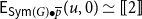 ${{\mathsf{E}}}_{\mathsf{Sym}(G) \bullet \overline{p}}(u,0) \simeq [\![ 2 ]\!]$
follows by applying
${{\mathsf{E}}}_{\mathsf{Sym}(G) \bullet \overline{p}}(u,0) \simeq [\![ 2 ]\!]$
follows by applying
 $(\bullet \overline{p})$
to
$(\bullet \overline{p})$
to
 $\mathsf{Sym}(G)$
. The case for
$\mathsf{Sym}(G)$
. The case for
 $x\equiv v$
and
$x\equiv v$
and
 $y\equiv n$
is analogous. Consequently, the edge sets coincide, confirming the expected isomorphism.
$y\equiv n$
is analogous. Consequently, the edge sets coincide, confirming the expected isomorphism.
Theorem 6.13. Let
 $\mathscr{M}$
represent a planar map of G,
$\mathscr{M}$
represent a planar map of G,
 $\mathscr{F}$
a specific face, and u and v two nodes on the boundary walk of
$\mathscr{F}$
a specific face, and u and v two nodes on the boundary walk of
 $\mathscr{F}$
. An extended planar map of
$\mathscr{F}$
. An extended planar map of
 $G \bullet p$
can be constructed from
$G \bullet p$
can be constructed from
 $\mathscr{M}$
, where p is situated onto
$\mathscr{M}$
, where p is situated onto
 $\mathscr{F}$
, splitting it into two faces.
$\mathscr{F}$
, splitting it into two faces.
The proof of Theorem 6.13 unfolds in several steps. We first define a map that extends
 $\mathscr{M}$
to a proper map of
$\mathscr{M}$
to a proper map of
 $G \bullet p$
with defined values for the nodes in p. Next, as illustrated in Fig. 12, we establish two faces resulting from placing p onto
$G \bullet p$
with defined values for the nodes in p. Next, as illustrated in Fig. 12, we establish two faces resulting from placing p onto
 $\mathscr{F}$
. The final step involves demonstrating that the candidate map for
$\mathscr{F}$
. The final step involves demonstrating that the candidate map for
 $G \bullet p$
is planar. That is, per Definition 6.6, that all pairs of walks in the symmetrisation of
$G \bullet p$
is planar. That is, per Definition 6.6, that all pairs of walks in the symmetrisation of
 $G \bullet p$
are walk-homotopic with respect to the given map.
$G \bullet p$
are walk-homotopic with respect to the given map.
Proof
of Theorem 6.13. Let
 $\mathscr{M}$
be a planar map of G,
$\mathscr{M}$
be a planar map of G,
 $\mathscr{F}$
a specific face, and u and v two nodes on the boundary walk of
$\mathscr{F}$
a specific face, and u and v two nodes on the boundary walk of
 $\mathscr{F}$
. We denote the graph
$\mathscr{F}$
. We denote the graph
 $G \bullet p$
as H and the prospective planar map for this graph as
$G \bullet p$
as H and the prospective planar map for this graph as
 $\mathscr{M'}$
. In the context of Definition 5.3, within the face walk boundary
$\mathscr{M'}$
. In the context of Definition 5.3, within the face walk boundary
 $\partial \mathscr{F}$
of the given face
$\partial \mathscr{F}$
of the given face
 $\mathscr{F}$
, we identify an edge preceding u, represented as
$\mathscr{F}$
, we identify an edge preceding u, represented as
 $a:{{\mathsf{E}}}_{G}(\mathsf{pred}(u),u)$
, and its succeeding edge
$a:{{\mathsf{E}}}_{G}(\mathsf{pred}(u),u)$
, and its succeeding edge
 $a^{+}:{{\mathsf{E}}}_{G}(u, \mathsf{suc}(u))$
. Analogously for v, we have
$a^{+}:{{\mathsf{E}}}_{G}(u, \mathsf{suc}(u))$
. Analogously for v, we have
 $b:{{\mathsf{E}}}_{G}(\mathsf{pred}(v),v)$
and
$b:{{\mathsf{E}}}_{G}(\mathsf{pred}(v),v)$
and
 $b^{+}:{{\mathsf{E}}}_{G}(v,\mathsf{suc}(v))$
, as depicted in Fig. 11(a).
$b^{+}:{{\mathsf{E}}}_{G}(v,\mathsf{suc}(v))$
, as depicted in Fig. 11(a).

Figure 11. Figure (a) in the caption illustrates the path addition
 $G \bullet p$
as detailed in Theorem 6.13. Figure (b) presents the planar map for G from Fig. 5(b), showcasing three graph extensions: the path addition of p, cyclic addition of q and spike addition of r. Though it is feasible to define the construction of r, it is not necessary for this discussion. The additions of p and q split faces
$G \bullet p$
as detailed in Theorem 6.13. Figure (b) presents the planar map for G from Fig. 5(b), showcasing three graph extensions: the path addition of p, cyclic addition of q and spike addition of r. Though it is feasible to define the construction of r, it is not necessary for this discussion. The additions of p and q split faces
 $F_2$
and
$F_2$
and
 $F_3$
from Fig. 5, generating two new faces each. The spike addition of r substitutes
$F_3$
from Fig. 5, generating two new faces each. The spike addition of r substitutes
 $F_4$
with a face of higher degree.
$F_4$
with a face of higher degree.
We define the map
 $\mathscr{M'}$
at each node x in H. We begin with the endpoints of p, that is,
$\mathscr{M'}$
at each node x in H. We begin with the endpoints of p, that is,
 $x = u$
and
$x = u$
and
 $x = v$
. For
$x = v$
. For
 $x = u$
, we alter the cycle
$x = u$
, we alter the cycle
 $\mathscr{M}(u)$
by introducing
$\mathscr{M}(u)$
by introducing
 $e_0$
between the edges a and
$e_0$
between the edges a and
 $a^{+}$
, resulting in the cycle
$a^{+}$
, resulting in the cycle
 $\mathscr{M'}(u) = (\cdot sa\,e_0\,a^{+}\cdot s)$
. Similarly, for
$\mathscr{M'}(u) = (\cdot sa\,e_0\,a^{+}\cdot s)$
. Similarly, for
 $x = v$
, the modified cycle
$x = v$
, the modified cycle
 $\mathscr{M'}(v)$
is
$\mathscr{M'}(v)$
is
 $(\cdot s b\,e_{n}\,b^{+}\cdot s)$
. For internal nodes of p, that is, nodes x in
$(\cdot s b\,e_{n}\,b^{+}\cdot s)$
. For internal nodes of p, that is, nodes x in
 $P_n$
, the map
$P_n$
, the map
 $\mathscr{M'}$
is defined directly. At each of these nodes, we encounter only two edges, denoted as
$\mathscr{M'}$
is defined directly. At each of these nodes, we encounter only two edges, denoted as
 $e_{i}$
and
$e_{i}$
and
 $e_{i+1}$
, where i ranges from 0 to
$e_{i+1}$
, where i ranges from 0 to
 $n-1$
. Remember that
$n-1$
. Remember that
 $e_0$
connects nodes u and 0,
$e_0$
connects nodes u and 0,
 $e_{n}$
links nodes
$e_{n}$
links nodes
 $n-1$
and v, and for the remaining,
$n-1$
and v, and for the remaining,
 $e_i$
bridges nodes
$e_i$
bridges nodes
 $i-1$
and i.
$i-1$
and i.
Assume the face
 $\mathscr{F}$
, induced by (A, h) of degree m according to Definition 5.3. Here, h is an edge-injective graph homomorphism from A to
$\mathscr{F}$
, induced by (A, h) of degree m according to Definition 5.3. Here, h is an edge-injective graph homomorphism from A to
 $\mathsf{Sym}(H)$
, satisfying the map-compatibility condition. Let
$\mathsf{Sym}(H)$
, satisfying the map-compatibility condition. Let
 $\partial \mathscr{F}$
be the boundary walk of
$\partial \mathscr{F}$
be the boundary walk of
 $\mathscr{F}$
of length k and define
$\mathscr{F}$
of length k and define
 $n_1,n_2$
as
$n_1,n_2$
as
 $k+(n+1)$
and
$k+(n+1)$
and
 $(m-k)+(n+1)$
, respectively.
$(m-k)+(n+1)$
, respectively.
Let us denote
 $F_1, F_2$
as faces induced by
$F_1, F_2$
as faces induced by
 $(C_{n_1}, h_1)$
and
$(C_{n_1}, h_1)$
and
 $(C_{n_2}, h_2)$
, respectively, where
$(C_{n_2}, h_2)$
, respectively, where
 $h_1 = (\alpha_1, \beta_1)$
and
$h_1 = (\alpha_1, \beta_1)$
and
 $h_2 =(\alpha_2, \beta_2)$
are morphisms of type
$h_2 =(\alpha_2, \beta_2)$
are morphisms of type
 $\mathsf{Hom}(C_{n_i},\mathsf{Sym}(H))$
for
$\mathsf{Hom}(C_{n_i},\mathsf{Sym}(H))$
for
 $i=1,2$
. The boundary walks of these faces,
$i=1,2$
. The boundary walks of these faces,
 $\partial F_1$
and
$\partial F_1$
and
 $\partial F_2$
, are defined as
$\partial F_2$
, are defined as
 $\mathsf{cw}_{\mathscr{F}}(u,v)\cdot \overrightarrow{p}$
and
$\mathsf{cw}_{\mathscr{F}}(u,v)\cdot \overrightarrow{p}$
and
 $\mathsf{ccw}_{\mathscr{F}}(u,v)\cdot \overrightarrow{p}$
, respectively. The subsequent image provides a visual representation of this concept.
$\mathsf{ccw}_{\mathscr{F}}(u,v)\cdot \overrightarrow{p}$
, respectively. The subsequent image provides a visual representation of this concept.
To establish the planarity of
 $\mathscr{M}'$
, we must first demonstrate that for each face
$\mathscr{M}'$
, we must first demonstrate that for each face
 $F_1$
and
$F_1$
and
 $F_2$
of
$F_2$
of
 $\mathscr{M}'$
,
$\mathscr{M}'$
,
 $h_1$
and
$h_1$
and
 $h_2$
satisfy the map-compatibility condition and uphold the edge-injectivity property. Beginning with
$h_2$
satisfy the map-compatibility condition and uphold the edge-injectivity property. Beginning with
 $h_1$
, consider the nodes in
$h_1$
, consider the nodes in
 $C_{n_1}$
, namely
$C_{n_1}$
, namely
 $0,1,\ldots,{n_1}-1$
. Each node
$0,1,\ldots,{n_1}-1$
. Each node
 $i : {{\mathsf{N}}}_{C_{n_1}}$
maps to a node defined by
$i : {{\mathsf{N}}}_{C_{n_1}}$
maps to a node defined by
 $\alpha$
from
$\alpha$
from
 $\mathscr{F}$
. Specifically,
$\mathscr{F}$
. Specifically,
 $\alpha_1(i)$
equals
$\alpha_1(i)$
equals
 $\alpha(i)$
for
$\alpha(i)$
for
 $i<k$
, while
$i<k$
, while
 $\alpha_(i)$
positions the node in
$\alpha_(i)$
positions the node in
 $\mathsf{cw}_{\mathscr{F}}(u,v)$
. For the corresponding edges,
$\mathsf{cw}_{\mathscr{F}}(u,v)$
. For the corresponding edges,
 $e:{{\mathsf{E}}}_{C_{n_1}}(i,i+1)$
, we employ the function
$e:{{\mathsf{E}}}_{C_{n_1}}(i,i+1)$
, we employ the function
 $\beta$
from
$\beta$
from
 $\mathscr{F}$
to define
$\mathscr{F}$
to define
 $\beta_1$
, such that
$\beta_1$
, such that
 $\beta_1(i,i+1,e)$
corresponds to
$\beta_1(i,i+1,e)$
corresponds to
 $\beta(i,i+1,e)$
.
$\beta(i,i+1,e)$
.
However, if
 $k\leq i \leq n_1$
, node i must be placed in
$k\leq i \leq n_1$
, node i must be placed in
 $\overline{p}$
, then
$\overline{p}$
, then
 $\alpha_1(i)$
is
$\alpha_1(i)$
is
 $n-i$
. Correspondingly, for edges, we set
$n-i$
. Correspondingly, for edges, we set
 $\beta_1(i,i+1,e)$
as the edge
$\beta_1(i,i+1,e)$
as the edge
 $\mathsf{inl}(e_{i})$
in
$\mathsf{inl}(e_{i})$
in
 $\mathsf{Sym}(H)$
. It is clear by construction that
$\mathsf{Sym}(H)$
. It is clear by construction that
 $h_1$
is an edge-injective, map-compatible graph homomorphism with the map
$h_1$
is an edge-injective, map-compatible graph homomorphism with the map
 $\mathscr{M'}$
, properties naturally inherited from h. In a similar vein, it can be proven that
$\mathscr{M'}$
, properties naturally inherited from h. In a similar vein, it can be proven that
 $h_2$
is well defined and fulfils the map-compatibility condition and the edge-injectivity property.
$h_2$
is well defined and fulfils the map-compatibility condition and the edge-injectivity property.
To prove that
 $\mathscr{M'}$
is planar, we must first show that it is spherical. To see this, we rely on Theorem 6.4, which allows us to apply the elimination of the propositional truncation to the evidence that
$\mathscr{M'}$
is planar, we must first show that it is spherical. To see this, we rely on Theorem 6.4, which allows us to apply the elimination of the propositional truncation to the evidence that
 $\mathscr{M}$
is spherical. This enables us to obtain a walk homotopy for any pair of walks in
$\mathscr{M}$
is spherical. This enables us to obtain a walk homotopy for any pair of walks in
 $\mathsf{Sym}(G)$
sharing endpoints, which is perhaps used henceforth without explicit mention. This entails that homotopic walks in
$\mathsf{Sym}(G)$
sharing endpoints, which is perhaps used henceforth without explicit mention. This entails that homotopic walks in
 $\mathsf{Sym}(G)$
, deforming along faces other than
$\mathsf{Sym}(G)$
, deforming along faces other than
 $\mathscr{F}$
, maintain their homotopy in
$\mathscr{F}$
, maintain their homotopy in
 $\mathsf{Sym}(H)$
. Therefore, our focus narrows down to:
$\mathsf{Sym}(H)$
. Therefore, our focus narrows down to:
-
(i) the set of walks in
$\mathsf{Sym}(G)$
deforming along
$\mathscr{F}$
, and -
(ii) the set of walks resulting from possible compositions of
$\overline{p}$
with existing walks in
$\mathsf{Sym}(G)$
.


For both walks originating from set (i), their homotopy is defined by the vertical composition of homotopies along
 $F_1$
and
$F_1$
and
 $F_2$
, as referenced in Theorem 6.2, (Prieto-Cubides 2022b, Section 5).
$F_2$
, as referenced in Theorem 6.2, (Prieto-Cubides 2022b, Section 5).
In case (ii), we consider walks without inner loops, following Lemma 5.8 in Prieto-Cubides (2022b). We examine three subcases without loss of generality, where the walk
 $\overline{p}$
from u to v decomposes into
$\overline{p}$
from u to v decomposes into
 $p_1$
and
$p_1$
and
 $p_2$
. Here,
$p_2$
. Here,
 $p_1$
is a walk from u to node y in
$p_1$
is a walk from u to node y in
 $\mathsf{Sym}(G \bullet p)$
, and
$\mathsf{Sym}(G \bullet p)$
, and
 $p_2$
from y to v, as shown in Fig. 13. Recall that a walk homotopy for any pair of walks in
$p_2$
from y to v, as shown in Fig. 13. Recall that a walk homotopy for any pair of walks in
 $\mathsf{Sym}(G)$
sharing endpoints is always accessible by hypothesis.
$\mathsf{Sym}(G)$
sharing endpoints is always accessible by hypothesis.

Figure 12. The figure demonstrates the partitioning of face
 $\mathscr{F}$
into two,
$\mathscr{F}$
into two,
 $F_1$
and
$F_1$
and
 $F_2$
, via
$F_2$
, via
 $G \bullet p$
when p resides on face
$G \bullet p$
when p resides on face
 $\mathscr{F}$
.
$\mathscr{F}$
.

Figure 13. The figure shows a part of the graph
 $\mathsf{Sym}(G\bullet p)$
embedded in the 2-sphere. As constructed in the proof of Theorem 6.13, the faces,
$\mathsf{Sym}(G\bullet p)$
embedded in the 2-sphere. As constructed in the proof of Theorem 6.13, the faces,
 $F_1$
and
$F_1$
and
 $F_2$
, of the map
$F_2$
, of the map
 $\mathscr{M'}$
are given by a face division of
$\mathscr{M'}$
are given by a face division of
 $\mathscr{F}$
by the path p. Such gives rise to new walk homotopies, as
$\mathscr{F}$
by the path p. Such gives rise to new walk homotopies, as
 $h_{F_1}$
and
$h_{F_1}$
and
 $h_{F_2}$
in the picture. The walk
$h_{F_2}$
in the picture. The walk
 $\overleftarrow{p}$
from u to v is the walk composition of
$\overleftarrow{p}$
from u to v is the walk composition of
 $p_1$
, a walk from u to y, and
$p_1$
, a walk from u to y, and
 $p_2$
, a walk from y to v. The walks
$p_2$
, a walk from y to v. The walks
 $\delta_1$
and
$\delta_1$
and
 $\delta_2$
are walks in
$\delta_2$
are walks in
 $\mathsf{Sym}(G)$
from x to z.
$\mathsf{Sym}(G)$
from x to z.
-
(a) Either
$w_1$
,
$w_2$
, or both, include
$\overleftarrow{p}$
as a subwalk from x to z. If
$w_1$
composes as
$\delta_1 \cdot \overleftarrow{p} \cdot \delta_2$
, and
$\overleftarrow{p}$
is not a subwalk of
$w_2$
, with
$\delta_1$
and
$\delta_2$
being walks in
$\mathsf{Sym}(G)$
from x to u and v to z, a homotopy of walks can be obtained as in the calculation below. The remaining cases are demonstrated similarly: -
(b) The walks
$w_1$
and
$w_2$
from x to y share a suffix (
$p_1$
) or a prefix (
$p_2$
). Without loss of generality, let
$w_1 = \delta_1 \cdot p_1$
and
$w_2 = \delta \cdot p_1$
, where
$\delta$
is a walk from x to u. These walks are homotopic in
$\mathsf{Sym}(G)$
via the spherical map
$\mathscr{M}$
, that is,
$\delta_1 \sim_{\mathscr{M}} \delta$
. The construction of
$\mathscr{M'}$
ensures
$\delta_1 \sim_{\mathscr{M}'} \delta$
. Utilising right whiskering, we deduce
$\delta_1 \cdot p_1 \sim_{\mathscr{M}'} \delta \cdot p_1$
, thereby reaching our desired conclusion. Similarly, if
$w_1$
is
$p_2\cdot \delta_2$
and
$w_2$
is
$p_2 \cdot \delta$
, where
$\delta$
is a walk from v to z, one can show that
$\delta_2 \sim_{\mathscr{M}} \delta$
, and hence
$\delta_2 \cdot p_2 \sim_{\mathscr{M}'} \delta \cdot p_2$
by left whiskering.


(c) The walks
 $w_1$
and
$w_1$
and
 $w_2$
from x to y can be expressed as composites of
$w_2$
from x to y can be expressed as composites of
 $\delta \cdot p_1$
and
$\delta \cdot p_1$
and
 $\delta' \cdot \overrightarrow{p_2}$
, respectively. Here,
$\delta' \cdot \overrightarrow{p_2}$
, respectively. Here,
 $\delta$
and
$\delta$
and
 $\delta'$
are walks from x to u and x to v, without sharing a common prefix or suffix subwalk. We aim to show
$\delta'$
are walks from x to u and x to v, without sharing a common prefix or suffix subwalk. We aim to show
 $w_1 \sim_{\mathscr{M}'} w_2$
via
$w_1 \sim_{\mathscr{M}'} w_2$
via
 $F_2$
deformation:
$F_2$
deformation:

Concluding our proof of Theorem 6.13, we have shown that
 $\mathscr{M}$
extends to a spherical map
$\mathscr{M}$
extends to a spherical map
 $\mathscr{M'}$
of
$\mathscr{M'}$
of
 $G\bullet p$
. By identifying
$G\bullet p$
. By identifying
 $F_1$
as the outer face, we further establish that
$F_1$
as the outer face, we further establish that
 $\mathscr{M'}$
is a planar map.
$\mathscr{M'}$
is a planar map.
Given that
 $\mathscr{M}$
is a planar map, we denote its planar extension derived from Theorem 6.13 by
$\mathscr{M}$
is a planar map, we denote its planar extension derived from Theorem 6.13 by
 $E(\mathscr{M}, \mathscr{F}, u, v,P_n)$
. To shorten the notation, this planar extension is denoted by
$E(\mathscr{M}, \mathscr{F}, u, v,P_n)$
. To shorten the notation, this planar extension is denoted by
 $E(\mathscr{M}, \mathscr{F}, p)$
, when the specifics of u, v and
$E(\mathscr{M}, \mathscr{F}, p)$
, when the specifics of u, v and
 $P_n$
are not really crucial to the discussion. We refer to this as the face division of
$P_n$
are not really crucial to the discussion. We refer to this as the face division of
 $\mathscr{F}$
by p, since this construction results in the placement of p in
$\mathscr{F}$
by p, since this construction results in the placement of p in
 $\mathscr{F}$
, dividing it into two new faces.
$\mathscr{F}$
, dividing it into two new faces.
Definition 6.14. For a finite graph G with map
 $\mathscr{M}$
, the Euler characteristic
$\mathscr{M}$
, the Euler characteristic
 $\chi_{\mathscr{M}}$
is defined as the number
$\chi_{\mathscr{M}}$
is defined as the number
 $v - e + f$
, where v, e and f denote the cardinalities of the sets of nodes, edges and faces, respectively:
$v - e + f$
, where v, e and f denote the cardinalities of the sets of nodes, edges and faces, respectively:
 \begin{equation}\chi_{\mathscr{M}} :=q v - e + f.\end{equation}
Theorem 6.15. For a graph G with planar map
 $\mathscr{M}$
, any planar extension of
$\mathscr{M}$
, any planar extension of
 $\mathscr{M}$
maintains Euler’s characteristic. That is, for any face
$\mathscr{M}$
maintains Euler’s characteristic. That is, for any face
 $\mathscr{F}$
of
$\mathscr{F}$
of
 $\mathscr{M}$
and nodes u, v within
$\mathscr{M}$
and nodes u, v within
 $\mathscr{F}$
connected by a path
$\mathscr{F}$
connected by a path
 $P_n$
, we have
$P_n$
, we have
 $\chi_{\mathscr{M}}$
equals
$\chi_{\mathscr{M}}$
equals
 $\chi_{E(\mathscr{M}, \mathscr{F}, u, v, P_n)}$
.
$\chi_{E(\mathscr{M}, \mathscr{F}, u, v, P_n)}$
.
Proof. The lemma follows from the construction detailed in the proof of Theorem 6.13. The path addition of
 $P_n$
between nodes u and v on face
$P_n$
between nodes u and v on face
 $\mathscr{F}$
increases the node count by
$\mathscr{F}$
increases the node count by
 $n+1$
, edges by
$n+1$
, edges by
 $n+2$
and faces by 1, preserving the Euler characteristic.
$n+2$
and faces by 1, preserving the Euler characteristic.
Euler characteristic serves as a planarity criterion for connected finite graphs. Specifically, according to Euler’s formula, a graph G is planar under the map
 $\mathscr{M}$
if and only if
$\mathscr{M}$
if and only if
 $\chi_{\mathscr{M}}$
equals 2. The constructions detailed in this section facilitate the verification of Euler’s formula for graphs constructed via path additions, an approach also employed later for biconnected planar graphs.
$\chi_{\mathscr{M}}$
equals 2. The constructions detailed in this section facilitate the verification of Euler’s formula for graphs constructed via path additions, an approach also employed later for biconnected planar graphs.
However, for arbitrary graphs not derived from graph extensions, validating Euler’s formula remains challenging, primarily due to the non-trivial task of determining the cardinality of the set of faces for an arbitrary map
 $\mathscr{M}$
of a given graph G, that is, computing the set of elements of type
$\mathscr{M}$
of a given graph G, that is, computing the set of elements of type
 $\mathsf{Face}(G,\mathscr{M})$
(see Definition 5.3). Progress was made by establishing that the type of faces forms a finite set. This suggests the feasibility of extracting this number in practice, possibly utilising the employed proof-assistant. We leave this to future work.
$\mathsf{Face}(G,\mathscr{M})$
(see Definition 5.3). Progress was made by establishing that the type of faces forms a finite set. This suggests the feasibility of extracting this number in practice, possibly utilising the employed proof-assistant. We leave this to future work.
6.5 Planar synthesis of graphs
Inductive graph construction methods abound, such as Whitney–Robbins synthesis, ear decomposition of a graph and the
 $K_4$
construction depicted in Fig. 14. Drawing inspiration from these methods and face divisions as in Theorem 6.13, we propose a method to build larger planar graphs using graph extensions, ensuring that we remain within the type of planar graphs.
$K_4$
construction depicted in Fig. 14. Drawing inspiration from these methods and face divisions as in Theorem 6.13, we propose a method to build larger planar graphs using graph extensions, ensuring that we remain within the type of planar graphs.

Figure 14. The figure illustrates a planar synthesis for constructing a
 $K_4$
planar map using a
$K_4$
planar map using a
 $C_3$
planar map. Initially, face
$C_3$
planar map. Initially, face
 $\mathscr{F}$
is divided into
$\mathscr{F}$
is divided into
 $F_1$
and
$F_1$
and
 $F_2$
. Subsequently,
$F_2$
. Subsequently,
 $F_1$
is split into
$F_1$
is split into
 $F_3$
and
$F_3$
and
 $F_4$
. The resulting map ends up with four faces, including the outer face.
$F_4$
. The resulting map ends up with four faces, including the outer face.
Definition 6.16. A Whitney synthesis (synthesis for short) of graph G from graph H is defined as a sequence of graphs
 $G_0,G_1, \cdot s, G_n$
, where
$G_0,G_1, \cdot s, G_n$
, where
 $G_0$
is H,
$G_0$
is H,
 $G_n$
is G, and each
$G_n$
is G, and each
 $G_i$
results from the path addition of
$G_i$
results from the path addition of
 $p_{i}$
to
$p_{i}$
to
 $G_{i-1}$
for i in the range 1 to n. Consequently, G can be viewed as the result of adding paths
$G_{i-1}$
for i in the range 1 to n. Consequently, G can be viewed as the result of adding paths
 $p_1, p_2, \cdot s, p_n$
to H:
$p_1, p_2, \cdot s, p_n$
to H:
 $$ G \equiv H \bullet p_1 \bullet p_2 \bullet \cdot s \bullet p_n .$$
The length of this synthesis is n. A simple synthesis refers to a sequence containing only simple additions. Conversely, a sequence composed solely of non-simple additions is termed a non-simple synthesis.
Theorem 6.17. Syntheses preserve graph-connectedness. Specifically, if a graph H is connected and G is synthesised from H, then each intermediate graph
 $G_i$
in the synthesis sequence is also connected.
$G_i$
in the synthesis sequence is also connected.
Proof. We prove this by induction on the length of the synthesis and the fact that path additions preserve connectedness, Theorem 6.11.
Definition 6.18. Given a planar map
 $\mathscr{M}$
of the graph H with outer face
$\mathscr{M}$
of the graph H with outer face
 $\mathscr{F}$
, we define a planar synthesis of G from H of length n as a sequence:
$\mathscr{F}$
, we define a planar synthesis of G from H of length n as a sequence:
 $$(G_0, \mathscr{M}_0, \mathscr{F}_0), (G_1, \mathscr{M}_1, \mathscr{F}_1)\cdot s, (G_n, \mathscr{M}_n, \mathscr{F}_n),$$
where
-
⊳
$(G_0, \mathscr{M}_0, \mathscr{F}_0)$
is equivalent to
$(H ,\mathscr{M}, \mathscr{F})$
, and -
⊳
$(G_n, \mathscr{M}_{n})$
corresponds to
$(G,E(\mathscr{M}_{n-1},\mathscr{F}_{n-1}, p_{n-1}))$
.


For each i in the range 1 to n, the graph
 $G_i$
is
$G_i$
is
 $G_{i-1} \bullet p_i$
, and the map
$G_{i-1} \bullet p_i$
, and the map
 $\mathscr{M}_i$
is
$\mathscr{M}_i$
is
 $E(\mathscr{M}_{i-1},\mathscr{F}_{i-1}, p_{i-1})$
, where
$E(\mathscr{M}_{i-1},\mathscr{F}_{i-1}, p_{i-1})$
, where
 $\mathscr{F}_{i-1}$
is a face of
$\mathscr{F}_{i-1}$
is a face of
 $\mathscr{M}_{i-1}$
.
$\mathscr{M}_{i-1}$
.
Theorem 6.19 If a graph G is synthesised from a planar graph H via planar synthesis, then G and every graph in the corresponding sequence are planar.
Proof. Through planar synthesis, each
 $G_i$
is derived from
$G_i$
is derived from
 $G_{i-1}$
via path addition, ensuring planarity by Theorem 6.11.
$G_{i-1}$
via path addition, ensuring planarity by Theorem 6.11.
While we have not yet employed non-simple additions, they have become relevant when we characterise planar biconnected graphs in the next section. It is possible to extend the face division theorem and its construction to utilise non-simple additions, Theorem 6.13, allowing us to adapt not only the planar synthesis in Definition 6.18 to non-simple planar syntheses but also Theorem 6.19 to accommodate non-simple additions. Hence, given a map
 $\mathscr{M}$
for G with a face
$\mathscr{M}$
for G with a face
 $\mathscr{F}$
, the corresponding planar map for
$\mathscr{F}$
, the corresponding planar map for
 $G \bullet \overline{p}$
is denoted as
$G \bullet \overline{p}$
is denoted as
 $E(\mathscr{M},\mathscr{F},\overline{p})$
, maintaining a similar notation as before. As with path additions, extending the map with non-simple additions introduces new faces.
$E(\mathscr{M},\mathscr{F},\overline{p})$
, maintaining a similar notation as before. As with path additions, extending the map with non-simple additions introduces new faces.
Taking into account
 $G \bullet_{u,v} \mathsf{Sym}(P_n)$
and the map
$G \bullet_{u,v} \mathsf{Sym}(P_n)$
and the map
 $E(\mathscr{M},\mathscr{F},\overline{p})$
, the number of faces increases to
$E(\mathscr{M},\mathscr{F},\overline{p})$
, the number of faces increases to
 $n+3$
, the number of nodes increases to
$n+3$
, the number of nodes increases to
 $v+n+1$
and the number of edges increases to
$v+n+1$
and the number of edges increases to
 $2\cdot (n+2)$
, as illustrated in Figure 15. Consequently, the Euler characteristic of
$2\cdot (n+2)$
, as illustrated in Figure 15. Consequently, the Euler characteristic of
 $E(\mathscr{M},\mathscr{F},\overline{p})$
is equal to the Euler characteristic of
$E(\mathscr{M},\mathscr{F},\overline{p})$
is equal to the Euler characteristic of
 $\mathscr{M}$
.
$\mathscr{M}$
.

Figure 15. The figure illustrates the face division of
 $\mathscr{F}$
by a non-simple path addition.
$\mathscr{F}$
by a non-simple path addition.
Consequently, the Euler characteristic of
 $E(\mathscr{M},\mathscr{F},\overline{p})$
is equal to the Euler characteristic of
$E(\mathscr{M},\mathscr{F},\overline{p})$
is equal to the Euler characteristic of
 $\mathscr{M}$
:
$\mathscr{M}$
:
 \begin{equation*} \chi_{E(\mathscr{M},\overline{p})} :\equiv (v + (n+1)) - (e + 2\cdot (n + 2)) + (f+(n+3)) \equiv \chi_{\mathscr{M}}.\end{equation*}
Fig. 13(b) demonstrates the construction of larger planar graphs using various path, cycle and spike additions. A spike addition to G, although not precisely defined here, as it is not extensively used for further constructions, can be essentially described as a path addition sharing only one node with G. With a given map for G, a simple addition of a spike creates a new face of a higher degree than the face where the spike is inserted. Consequently, non-simple spike additions also increase the number of faces for the extended map due to the emergence of new faces between edge pairs that share endpoints.
The remainder of this section aims to characterise the construction of all 2-connected planar graphs. In general, a graph is k-connected if it cannot be disconnected by removing less than k nodes. Depending on k, there are various methods to construct the set of k-connected graphs. For instance, any undirected 2-connected graph can be constructed by applying path additions to an appropriate cyclic graph (Diestel Reference Diestel2012, Section 3). Our focus in the following will be on the construction of 2-connected planar graphs.
Definition 6.20. A graph G is defined as 2-connected, or biconnected, when the proposition
 $\mathsf{Biconnected}(G)$
holds. This is, when the resulting graph
$\mathsf{Biconnected}(G)$
holds. This is, when the resulting graph
 $G - x$
, formed by removing a node x from G, remains connected.
$G - x$
, formed by removing a node x from G, remains connected.
Specifically,
 $G - x$
is the graph made up of the set of nodes,
$G - x$
is the graph made up of the set of nodes,
 $\Sigma_{y : {{\mathsf{N}}}_{G}} (x \neq y)$
, and their corresponding edges in G:
$\Sigma_{y : {{\mathsf{N}}}_{G}} (x \neq y)$
, and their corresponding edges in G:
 \begin{equation*} \mathsf{Biconnected}(G):\equiv \prod_{(x\,:\,{{\mathsf{N}}}_{G})}\, \mathsf{Connected}(G - x). \end{equation*}
Theorem 6.21. If G is a cyclic graph, then
 $\mathsf{Sym}(G)$
is 2-connected.
$\mathsf{Sym}(G)$
is 2-connected.
Proof. The cyclic nature of G ensures that in
 $\mathsf{Sym}(G)$
, there are two inner loop-free walks between any pair of nodes: a direct walk following the cycle of G and a reverse walk counter to the cycle. These walks are edge-disjoint and thus preserve the graph’s connectivity despite the removal of any single node-only one of the walks might be affected, leaving the other intact to sustain connectedness.
$\mathsf{Sym}(G)$
, there are two inner loop-free walks between any pair of nodes: a direct walk following the cycle of G and a reverse walk counter to the cycle. These walks are edge-disjoint and thus preserve the graph’s connectivity despite the removal of any single node-only one of the walks might be affected, leaving the other intact to sustain connectedness.
The property of 2-connectedness in a graph does not remain invariant under simple path additions. Clearly, removing a node from the added path p disconnects
 $G \bullet p$
. Yet, through non-simple path additions, it is possible to maintain and even augment 2-connected graphs.
$G \bullet p$
. Yet, through non-simple path additions, it is possible to maintain and even augment 2-connected graphs.
Theorem 6.22. Let G denote a 2-connected graph. The graph extensions,
 $G \bullet\overline{p}$
and
$G \bullet\overline{p}$
and
 $\mathsf{Sym}(G) \bullet \overline{p}$
, preserve the 2-connected graph property.
$\mathsf{Sym}(G) \bullet \overline{p}$
, preserve the 2-connected graph property.
Proof. To show that
 $G \bullet_{u,v} \mathsf{Sym}(P_n) - x$
remains connected for any node x in
$G \bullet_{u,v} \mathsf{Sym}(P_n) - x$
remains connected for any node x in
 $G \bullet \overline{p}$
, we consider the location of x. If x is within G, then
$G \bullet \overline{p}$
, we consider the location of x. If x is within G, then
 $G - x$
is connected by hypothesis. Applying Theorem 6.11, it follows that
$G - x$
is connected by hypothesis. Applying Theorem 6.11, it follows that
 $G \bullet\overline{p} - x$
is also connected, showing the 2-connectivity of
$G \bullet\overline{p} - x$
is also connected, showing the 2-connectivity of
 $G \bullet\overline{p}$
. Otherwise, if x lies on
$G \bullet\overline{p}$
. Otherwise, if x lies on
 $\overline{p}$
, its removal divides
$\overline{p}$
, its removal divides
 $\overline{p}$
into two parts,
$\overline{p}$
into two parts,
 $p_1$
and
$p_1$
and
 $p_2$
. For any two nodes in
$p_2$
. For any two nodes in
 $G \bullet\overline{p} - x$
, we show they are connected. If both nodes are in G or the same part
$G \bullet\overline{p} - x$
, we show they are connected. If both nodes are in G or the same part
 $p_i$
, they are connected by prior arguments or direct traversal, respectively. If they are located in distinct subgraphs, say x is in
$p_i$
, they are connected by prior arguments or direct traversal, respectively. If they are located in distinct subgraphs, say x is in
 $p_1$
and y is in
$p_1$
and y is in
 $p_2$
. We can construct a walk from x to u, another walk across G from u to v (since G is connected), and then to the second node, Hence,
$p_2$
. We can construct a walk from x to u, another walk across G from u to v (since G is connected), and then to the second node, Hence,
 $G \bullet \overline{p}$
maintains 2-connectivity.
$G \bullet \overline{p}$
maintains 2-connectivity.
Inspired by Yamamoto’s work (Yamamoto et al. Reference Yamamoto, Thomas Schubert, Windley and Alves-Foss1995), our focus is on the construction of 2-connected planar graphs. Within a different theoretical setting (HOL) and using a different graph definition, Yamamoto shows that any undirected 2-connected planar graph can be inductively built by adding diverse paths to circuits (their term for cyclic graphs). In our context, we initiate constructions with any 2-connected graph
 $\mathsf{Sym}(C_n)$
and subsequently extend these graphs by non-simple planar additions.
$\mathsf{Sym}(C_n)$
and subsequently extend these graphs by non-simple planar additions.
Theorem 6.23. In a non-simple Whitney synthesis of G originating from a 2-connected graph H, with planarity ensured by a map
 $\mathscr{M}$
, each graph in the synthesis maintains 2-connectivity and planarity via planar extension of
$\mathscr{M}$
, each graph in the synthesis maintains 2-connectivity and planarity via planar extension of
 $\mathscr{M}$
using non-simple additions.
$\mathscr{M}$
using non-simple additions.
Proof. Assuming a non-simple Whitney synthesis of G from H of length n is given, we proceed by induction on n.
-
⊳ Base case (
$n=0$
). The graph G is H, and by hypothesis, H is a 2-connected planar graph. Thus, the conclusion follows. -
⊳ Inductive step. For the inductive step, we assume that the claim holds for a sequence of length n, thus establishing
$G_n$
as a 2-connected planar graph via map
$\mathscr{M}_n$
. We then aim to demonstrate that G, defined as
$G_n \bullet \overline{p_i}$
for some path
$p_i$
, also qualifies as a 2-connected planar graph. -
⊳ Given that
$G_n$
is 2-connected, it follows from Theorem 6.22 that
$G_n \bullet \overline{p_i}$
also retains this property. We then extend the planar map
$\mathscr{M}_n$
of
$G_n$
to a planar map
$\mathscr{M}$
for G, preserving the outer face or selecting a new outer face from the additions. This construction of
$\mathscr{M}$
follows the method in Theorem 6.13, where we expand planar maps using simple additions, as required here.


Theorem 6.24. Any graph synthesised from
 $\mathsf{Sym}(C_n)$
through non-simple Whitney syntheses is a 2-connected planar graph.
$\mathsf{Sym}(C_n)$
through non-simple Whitney syntheses is a 2-connected planar graph.
Proof. Given that
 $C_n$
is planar by Example 6.8 and consequently connected,
$C_n$
is planar by Example 6.8 and consequently connected,
 $\mathsf{Sym}(C_n)$
is 2-connected by Theorem 6.21. By repeatedly applying Theorem 6.23 to each step in the given synthesis sequence, we ensure the resulting graph’s 2-connectivity and planarity.
$\mathsf{Sym}(C_n)$
is 2-connected by Theorem 6.21. By repeatedly applying Theorem 6.23 to each step in the given synthesis sequence, we ensure the resulting graph’s 2-connectivity and planarity.
Lemma 3 and Proposition 4 in Yamamoto et al. (Reference Yamamoto, Thomas Schubert, Windley and Alves-Foss1995) discuss undirected 2-connected planar graphs similar to the converse of Theorem 6.24. It is possible to follow Yamamoto’s argument closely, even though it was presented in an informal way. However, this requires preliminary formalisation of several technicalities, such as maximal subgraphs, adjacent faces and edge sequence deletion. Subsequently, one can assert that non-simple Whitney syntheses entirely determine 2-connected planar graphs, as expressed similarly in Diestel (Reference Diestel2012, Section 3). In essence, any graph defined as planar in Definition 6.6 and 2-connected in Definition 6.20 can be inductively generated from
 $\mathsf{Sym}(C_n)$
via iterative non-simple path additions and proper map extensions.
$\mathsf{Sym}(C_n)$
via iterative non-simple path additions and proper map extensions.
Further exploration of graph extensions, such as amalgamations, appendages, deletions, contractions and subdivisions, should be considered to generate planar graphs (Gross et al. Reference Gross, Yellen and Anderson2018, Section 7.3).
7. Related Work
The study of planar graphs and more general graph-theoretic topics can be found in relevant projects and large libraries formalised in Coq (Doczkal and Pous Reference Doczkal and Pous2020), Isabelle/HOL (Noschinski Reference Noschinski2015), and most recently, in Agda (Rijke et al. Reference Rijke, Bonnevier, Prieto-Cubides and Bakke2023), and Lean (The Mathlib Community 2020). Examples of notable projects on the subject include the formal proof of the Four-Colour Theorem (FCT) in Coq (Gonthier Reference Gonthier2008), the proof of the discrete form of the Jordan Curve Theorem in Coq (Dufourd and Puitg Reference Dufourd and Puitg2000), and the verification of Kepler’s Conjecture in HOL (Hales et al. Reference Hales, Adams and Bauer2017).
Different approaches have been proposed to address the planarity of graphs in formal systems. These works use different mathematical objects depending on the system. We use combinatorial maps in this work, but other related constructions are, for example, root maps defined in terms of permutations (Dubois et al. Reference Dubois, Giorgetti, Genestier, Aichernig and Furia2016) and hypermaps (Dufourd Reference Dufourd2009; Dufourd and Puitg Reference Dufourd and Puitg2000; Gonthier Reference Gonthier2008), among others. In particular, one can see that the notion of a hypermap is a generalisation of a combinatorial map for undirected finite graphs. Such a concept is one fundamental construction to formalise mathematics of graph maps amongst in theorem provers, along with the computer-checked proof of FCT. Additionally, Dufourd states and proves the Euler’s polyhedral formula and the Jordan Curve Theorem using an inductive characterisation of hypermaps (Dufourd Reference Dufourd2009; Dufourd and Puitg Reference Dufourd and Puitg2000). Recently, for a more standard representation of finite graphs, Doczkal proved that, according to his notion of a plane map based on hypermaps, every
 $K_{3,3}$
-free graph and
$K_{3,3}$
-free graph and
 $K_{5}$
-free graph without isolating nodes is planar, a direction of Wagner’s theorem (Doczkal Reference Doczkal2021).
$K_{5}$
-free graph without isolating nodes is planar, a direction of Wagner’s theorem (Doczkal Reference Doczkal2021).
An alternate strategy for planar graphs is to build them iteratively. For example, in Yamamoto et al. (Reference Yamamoto, Thomas Schubert, Windley and Alves-Foss1995), the authors showed that any biconnected and finite planar graph can be decomposed as a finite set of cycle graphs, where every face is the region bounded by a closed walk (Gross et al. Reference Gross, Yellen and Anderson2018, Sections 5.2, 7.3). This construction defines an inductive data type that begins with a cycle graph
 $C_n$
serving as the base case, and by repeatedly merging new instances of cycle graphs, one gets the final planar graph. Bauer formalises in Isabelle/HOL a similar construction of planar graphs from a set of faces (Bauer and Nipkow 2002; Bauer Reference Bauer2005). A related approach in our setting is of the treatment of planar graph extensions, as described in Section 6.4.
$C_n$
serving as the base case, and by repeatedly merging new instances of cycle graphs, one gets the final planar graph. Bauer formalises in Isabelle/HOL a similar construction of planar graphs from a set of faces (Bauer and Nipkow 2002; Bauer Reference Bauer2005). A related approach in our setting is of the treatment of planar graph extensions, as described in Section 6.4.
To our knowledge, previous work in type theory related to graph planarity has been conducted within different formal systems and for distinct classes and notions of graphs. These studies predominantly define planarity for undirected finite graphs. In contrast, our definition encompasses the broader class of connected and locally finite directed multigraphs. Our research aligns more closely with the foundations of mathematics, particularly the formalisation of mathematics in HoTT, rather than the practical aspects of graph theory. This necessitates proposing new constructs, occasionally even for the most fundamental concepts within the theory.
8. Concluding Remarks
This document is a case study of graph-theoretic concepts in constructive mathematics using HoTT. An elementary characterisation of planarity of connected and locally finite directed multigraphs is presented in Section 6.3. We collected all the maps of a graph in the two-dimensional plane – identified up to isotopy – in a homotopy set, see Theorem 6.7. The type of these planar maps displays some of our main contributions, for example, the type of spherical maps stated in Definition 6.3 and the type of faces for a given map in Definition 5.3. As far as we know, the presentation of these types in a dependent type theory like HoTT is novel. For example, besides its rather technical definition, we believe the type of faces encodes in a better combinatorial way the essence of the topological intuition behind it, rather than, being defined as simply cyclic lists of nodes, as by other authors (Bauer Reference Bauer2005; Gonthier Reference Gonthier2008; Yamamoto et al. Reference Yamamoto, Thomas Schubert, Windley and Alves-Foss1995), see Section 5. We did not include a proof that the type of faces of a map of a finite graph is finite. We omitted it here due to its technical complexity, involving multiple applications of finiteness results and identification of convenient equivalences. This detailed proof is included in an upcoming thesis by the first author, an extended version of this work and related formalisations in Agda.
Additionally, as a way to construct planar graphs inductively, we presented extensions for planar maps. We demonstrated that any cycle graph is planar, and by means of planar extensions such as path additions, one can construct larger planar graphs; for example, to illustrate this approach, a planar map for
 $K_4$
using simply path additions from a planar map of
$K_4$
using simply path additions from a planar map of
 $C_3$
is illustrated in Fig. 14. Other relevant notions for this work are cyclic types, cyclic graphs, homotopy for walks (Prieto-Cubides 2022b) and spherical maps.
$C_3$
is illustrated in Fig. 14. Other relevant notions for this work are cyclic types, cyclic graphs, homotopy for walks (Prieto-Cubides 2022b) and spherical maps.
We chose HoTT as the reasoning framework to directly study the symmetry of our mathematical constructions. Many of the proofs supporting our development could only be constructed by adopting the UA, a main principle in HoTT. A primary example of using Univalence in this paper is the structural identity principle for graphs, as stated in Theorem 3.7.
Another contribution of this work includes the (computer-checked) proofs. Not all but the relevant concepts in this document have been formalised in the proof assistant Agda, in a fully self-contained development (Prieto-Cubides 2022a). However, for technical reasons, the formalisation of Example 6.8 and further in-depth studies on the main results in Section 6.4 like Theorems 6.13 and 6.24 are left for future work.
This work can serve as a starting point for further developments of graph theory in HoTT or related dependently typed theories. We expect further research to provide other interesting results, such as the equivalences between different characterisations of planarity for graphs, for example, the Kuratowski’s and Wagner’s characterisations for planar graphs, and the realisation of planar graphs defined via HITs.
Acknowledgements
We express our gratitude to the anonymous reviewers and Marc Bezem, whose insightful comments significantly enhanced this paper. Our thanks also extend to the organisers of TYPES2019 and the referees for their valuable critique on our initial presentation of the backbone of this work. The first author would like to express appreciation to the organisers of the Midlands Graduate School 2019 and particularly to Noam Zeilberger for engaging discussions on rooted maps, planarity criteria and an early version of this work. Thanks to Benjamin Chetioui and Tam Thanh Truong for their assistance in proofreading earlier drafts. Lastly, we acknowledge the unwavering support of the Agda Team in maintaining the Agda proof assistant.

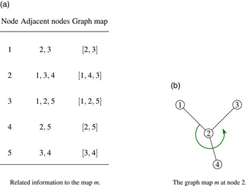
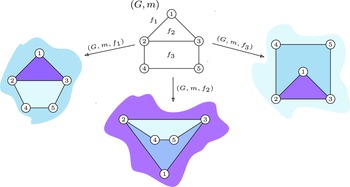


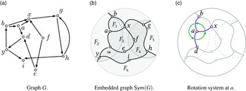


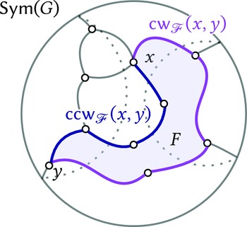


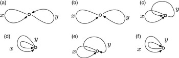


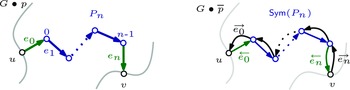


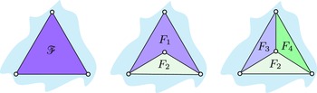


 Open access