


1. Introduction
A majority of currently popular classification models map a specific input $\boldsymbol{x}$
(e.g., a token or a sentence) to an output
$\boldsymbol{x}$
(e.g., a token or a sentence) to an output $\hat{\boldsymbol{y}}$
(Bishop Reference Bishop2006) where
$\hat{\boldsymbol{y}}$
(Bishop Reference Bishop2006) where $\hat{\boldsymbol{y}}$
can be a class, a sequence (e.g., a generated text) or an answer span extracted from a text context, for example. Typically, the
$\hat{\boldsymbol{y}}$
can be a class, a sequence (e.g., a generated text) or an answer span extracted from a text context, for example. Typically, the $\boldsymbol{x} \rightarrow \hat{\boldsymbol{y}}$
mapping involves various modulations and abstractions of
$\boldsymbol{x} \rightarrow \hat{\boldsymbol{y}}$
mapping involves various modulations and abstractions of $\boldsymbol{x}$
in a latent space (e.g., hidden layers of a neural network) but does not support variations or trajectories of
$\boldsymbol{x}$
in a latent space (e.g., hidden layers of a neural network) but does not support variations or trajectories of $\hat{\boldsymbol{y}}$
.Footnote a Humans, on the other hand, rarely come to a single decision right away but follow a complex thought process that involves reflecting on initial decisions (taking into consideration various constraints, such as knowledge, beliefs, and intuition), comparing different hypotheses, or resolving contradictions.
$\hat{\boldsymbol{y}}$
.Footnote a Humans, on the other hand, rarely come to a single decision right away but follow a complex thought process that involves reflecting on initial decisions (taking into consideration various constraints, such as knowledge, beliefs, and intuition), comparing different hypotheses, or resolving contradictions.
While the human “trains-of-thought” process has been studied extensively in cognitive sciences and philosophy—one particular example being Hegel’s dialectics (Maybee Reference Maybee2020)—“trains-of-thought” theories have not been further explored by the machine learning community. However, with increasingly complex tasks that have large output spaces (such as question answering (QA)Footnote b), or tasks that require multiple reasoning steps (such as multi-hop QA), pose nontrivial practical challenges because learning to directly hit the right prediction in one shot might be more difficult than to learn to self-correct an initial prediction iteratively.
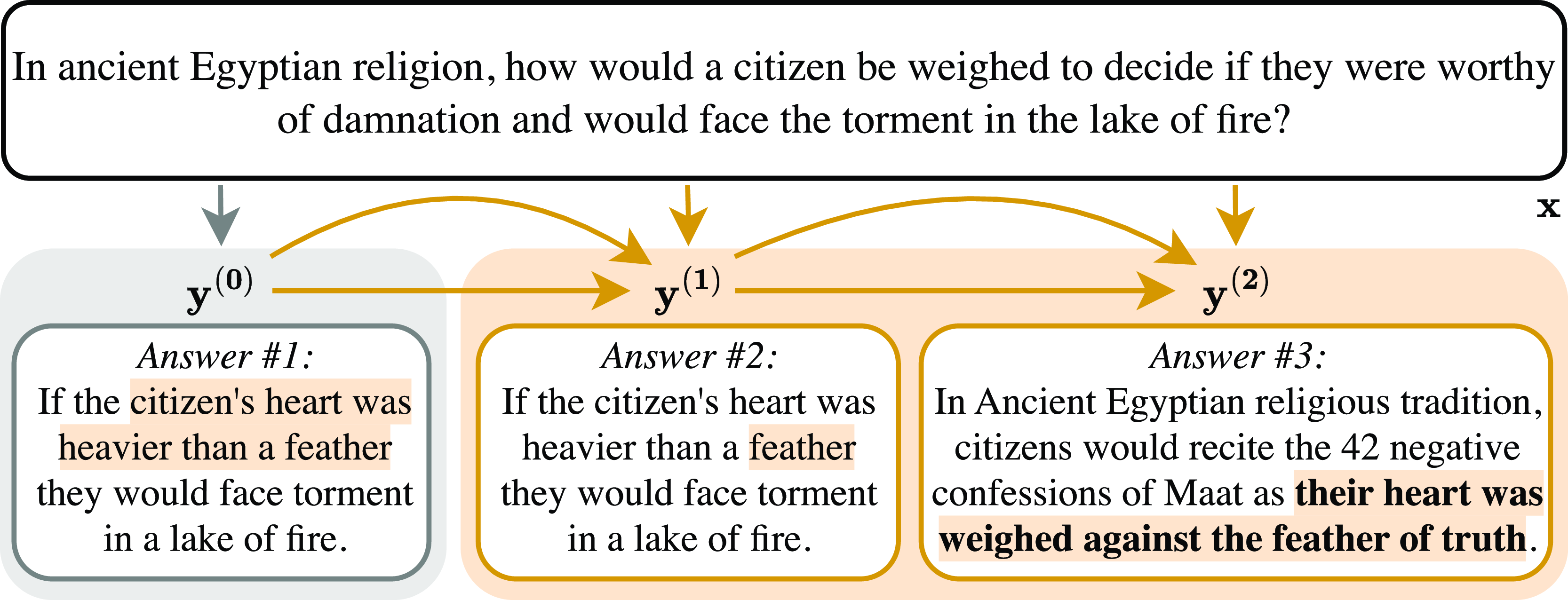
Figure 1. In contrast to the vanilla approach of mapping an input to an output in a single step (grey box), we propose a method that allows models to sequentially “reconsider” and update their predictions through a “thought flow” extension which can correct an incorrect (false) answer. In this (real) QA example, the orange box marks our thought flow extension, which corrects a flawed answer in two steps and ultimately returns the correct ground-truth answer (marked in bold).
In this paper, we propose and evaluate a “thought flow” method for iterative self-correction of predictions via sequences of interdependent probability distributions with the goal of (a) increasing prediction performance and (b) providing a perspective onto the model’s “reasoning” path that can provide explanatory value to humans. Furthermore, we propose a simple correction module to implement this concept. It can be used on top of any model that provides output logits of one or multiple distributions. In particular, it is inspired by the three moments of Hegel’s dialectics which we map onto forward and backward passes in a model architecture, trained to judge whether the predicted class distribution corresponds to a correct prediction.
In our experiments on QA, we demonstrate our method’s ability to self-correct incorrect (false) answer span predictions and identify qualitative patterns of self-correction, such as answer span reductions or extensions. Fig. 1 shows a real example of a thought flow which corrects a prediction ( $\mathbf{y^{(0)}}$
) output by a standard model to a new prediction (
$\mathbf{y^{(0)}}$
) output by a standard model to a new prediction ( $\mathbf{y^{(2)}}$
) via two steps, namely an answer span reduction and a cross-sentence answer jump. We find that our method can improve performance by up to 9.6% (absolute) in
$\mathbf{y^{(2)}}$
) via two steps, namely an answer span reduction and a cross-sentence answer jump. We find that our method can improve performance by up to 9.6% (absolute) in $\text{F}_1$
on a QA data set.
$\text{F}_1$
on a QA data set.
Finally, we assess the impact of thought flow predictions on human users within a crowdsourcing study. We find that thought flow predictions are perceived as significantly more correct, understandable, helpful, natural, and intelligent than single-answer predictions and/or top-3 predictions and they result in the overall best user performance without increasing completion times or mental effort.
In summary, our main contributions consist of (i) a formalization of a “thought flow” concept inspired by Hegel’s dialectics, (ii) a novel correction module and a corresponding gradient-based update scheme to incorporate a thought flow into state-of-the-art Transformer networks, (iii) experiments on QA that demonstrate its strong correction capabilities and identify qualitative patterns of self-correction, (iv) a crowdsourcing user study that demonstrates that thought flows can improve perceived system performance as well as actual real-world user performance using the system, and (v) a demonstration of how our thought flow method can be applied beyond natural language processing using the example of a vision task.
2. Thought flow networks
In this section, we present background on Hegel’s dialectics (Section 2.1), formalize thought flows based on it (Section 2.2), and describe a concrete implementation for QA (Section 2.3).
2.1 Inspiration: Hegel’s dialectics
Drawing inspiration from Hegel’s dialectics, our proposed method enables an existing model architecture to reflect and refine its predictions. In the following, we introduce the fundamental notion of the three “moments” in Hegel’s dialectics and describe how we designed our thought flow concept. We provide further background on Hegel’s dialectics in Appendix A.
Hegel’s dialectics distinguishes three moments: (i) the moment of understanding, (ii) the dialectical moment, and (iii) the speculative moment. The moment of understanding refers to the initial, “seemingly stable” determination of a concept, object, or idea. In the second moment, the ostensible stability is lost due to the one-sidedness or restrictedness of the initial determination causing it to sublate Footnote c itself into its own negation. The speculative moment ultimately unifies and resolves the contradictory determinations by negating the contradiction (Maybee Reference Maybee2020).Footnote d
2.2 Formalization of thought flow concept
We now translate the high-level description of these three moments into a simplified mathematical setting that can be implemented in any (neural) model that uses a vector-valued representation of the input (such as an embedding) and outputs (tuples of) logits. In particular, we formalize and embed Hegel’s dialectics in a framework with which we can obtain an initial “thought” vector and update it iteratively via the three “moments.” Table 1 provides an overview of these moments and their corresponding elements in our thought flow method. In the following, we discuss these in detail.
Note that our formalization of Hegel’s dialectics is approximative in nature, intended to inspire the development of novel machine learning models in general and thought flow nets in particular. For a detailed discussion of a formalization of Hegel’s Dialectics and its logical status, we refer to, i.a., Ficara and Priest (Reference Ficara and Priest2023), Nuzzo (Reference Nuzzo2023), and Priest (Reference Priest2023).
Thought. We represent a thought as $\hat{\boldsymbol{z}} \in Z$
, a vector of logits corresponding to a model’s prediction and
$\hat{\boldsymbol{z}} \in Z$
, a vector of logits corresponding to a model’s prediction and $Z \subseteq \mathbb{R}^c$
being the logit space of a prediction.Footnote e
$Z \subseteq \mathbb{R}^c$
being the logit space of a prediction.Footnote e $\hat{\boldsymbol{z}}$
serves as a representation of the model’s “decision state” as it captures implicit information about the most probable output (i.e., the decision itself) but also possible alternatives and uncertainty estimates encoded in the respective probability distribution. We want to emphasize that this representation of a “thought” should be understood as a metaphor that is necessarily lossy and simplistic and not as a neurologically plausible description.
$\hat{\boldsymbol{z}}$
serves as a representation of the model’s “decision state” as it captures implicit information about the most probable output (i.e., the decision itself) but also possible alternatives and uncertainty estimates encoded in the respective probability distribution. We want to emphasize that this representation of a “thought” should be understood as a metaphor that is necessarily lossy and simplistic and not as a neurologically plausible description.
Moment of Understanding. The first moment relates to an initial, seemingly stable determination of a concept, object, or idea in the model. We capture the moment of understanding through the initial value of $\hat{\boldsymbol{z}}^{(\textbf{0})}$
, which is the output of a prediction function
$\hat{\boldsymbol{z}}^{(\textbf{0})}$
, which is the output of a prediction function $f_{\text{pred}}\,:\, \Phi \rightarrow Z$
applied to a model with an encoded input
$f_{\text{pred}}\,:\, \Phi \rightarrow Z$
applied to a model with an encoded input $\phi (\mathbf{x})$
, an encoding function
$\phi (\mathbf{x})$
, an encoding function $\phi \,:\, \mathbb{R^d} \rightarrow \Phi$
, and an encoding space
$\phi \,:\, \mathbb{R^d} \rightarrow \Phi$
, and an encoding space $\Phi \subseteq \mathbb{R}^e$
(see Fig. 2(a)) where
$\Phi \subseteq \mathbb{R}^e$
(see Fig. 2(a)) where $e$
denotes the dimensionality of the encoding space. Concretely, our formalization of the moment of understanding thus is the first model prediction represented as a probability distribution over the class labels.Footnote f
$e$
denotes the dimensionality of the encoding space. Concretely, our formalization of the moment of understanding thus is the first model prediction represented as a probability distribution over the class labels.Footnote f
Table 1. Overview of the concepts from Hegel’s dialectics which we draw inspiration from (left), their main characteristics (middle), and their corresponding elements in our proposed thought flow method (right)
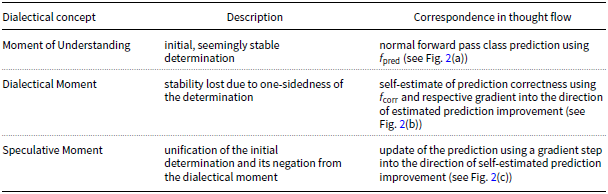
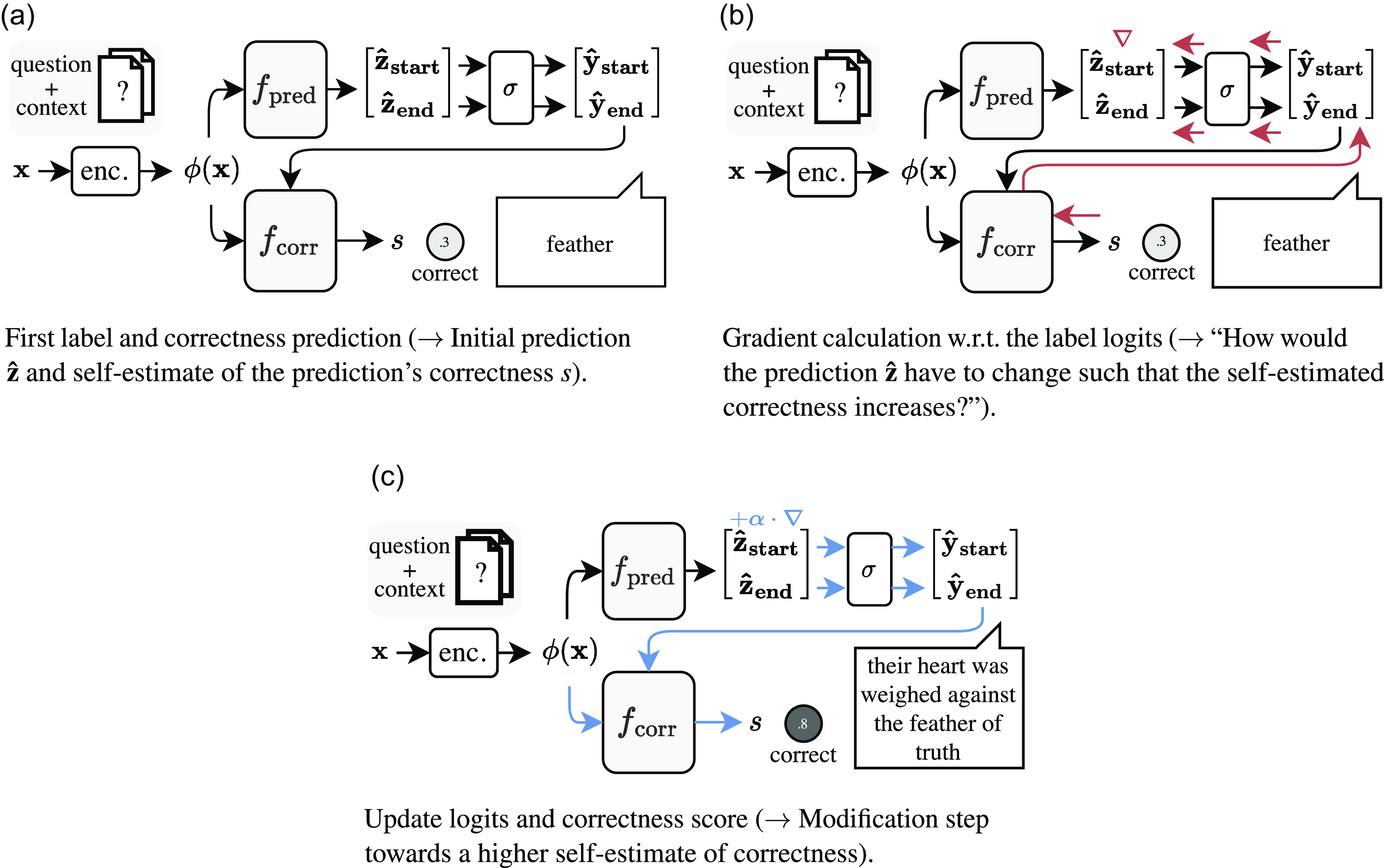
Figure 2. The steps of our prediction update scheme. The example shows the second answer change from Fig. 1. $\boldsymbol{x}$
refers to the model input and represents the question and its given textual context, “enc.” denotes an encoder function (e.g., a Transformer model),
$\boldsymbol{x}$
refers to the model input and represents the question and its given textual context, “enc.” denotes an encoder function (e.g., a Transformer model), $f_{\text{pred}}$
maps the encoding
$f_{\text{pred}}$
maps the encoding $\phi (\boldsymbol{x})$
to logits that correspond to probability distributions over start and end positions of the respectively predicted answer. In addition to this standard model architecture, we propose the addition of a function
$\phi (\boldsymbol{x})$
to logits that correspond to probability distributions over start and end positions of the respectively predicted answer. In addition to this standard model architecture, we propose the addition of a function $f_{\text{corr}}$
that is trained to predict an estimate of a correctness score
$f_{\text{corr}}$
that is trained to predict an estimate of a correctness score $s$
(e.g.,
$s$
(e.g., $\text{F}_1$
score) given
$\text{F}_1$
score) given $\phi (\boldsymbol{x})$
and the probability distributions predicted by
$\phi (\boldsymbol{x})$
and the probability distributions predicted by $f_{\text{pred}}$
.
$f_{\text{pred}}$
.
Dialectical Moment. At the second moment, the determination of the concept, object, or idea becomes unstable due to the initial determination’s one-sidedness or restrictedness. To model this, we apply a new function $f_{\text{corr}}\,:\, Z \times \Phi \rightarrow \mathbb{R}$
that differentiably maps
$f_{\text{corr}}\,:\, Z \times \Phi \rightarrow \mathbb{R}$
that differentiably maps $\hat{\boldsymbol{z}}^{(\textbf{0})}$
to a correctness score
$\hat{\boldsymbol{z}}^{(\textbf{0})}$
to a correctness score $s \in \mathbb{R}$
which is an estimate of the quality of the model prediction corresponding to
$s \in \mathbb{R}$
which is an estimate of the quality of the model prediction corresponding to $\hat{\boldsymbol{z}}^{(\textbf{0})}$
while being conditioned on
$\hat{\boldsymbol{z}}^{(\textbf{0})}$
while being conditioned on $\phi (\boldsymbol{x})$
. Intuitively,
$\phi (\boldsymbol{x})$
. Intuitively, $f_{\text{corr}}(\hat{\boldsymbol{z}}^{(\textbf{0})}, \phi (\boldsymbol{x}))$
quantifies an estimate of how good the current prediction corresponding to
$f_{\text{corr}}(\hat{\boldsymbol{z}}^{(\textbf{0})}, \phi (\boldsymbol{x}))$
quantifies an estimate of how good the current prediction corresponding to $\hat{\boldsymbol{z}}^{(\textbf{0})}$
is given the model input corresponding to
$\hat{\boldsymbol{z}}^{(\textbf{0})}$
is given the model input corresponding to $\phi (\boldsymbol{x})$
. Note that
$\phi (\boldsymbol{x})$
. Note that $f_{\text{corr}}$
does not have access to the (unknown) ground-truth label, but only relies on the predicted logits and the input representation. Intuitively,
$f_{\text{corr}}$
does not have access to the (unknown) ground-truth label, but only relies on the predicted logits and the input representation. Intuitively, $f_{\text{corr}}$
thus quantifies how plausible the combination of the prediction
$f_{\text{corr}}$
thus quantifies how plausible the combination of the prediction $\hat{\boldsymbol{z}}^{(\textbf{0})}$
and the encoded input
$\hat{\boldsymbol{z}}^{(\textbf{0})}$
and the encoded input $\phi (\boldsymbol{x})$
is. This quantification can rely on (a) individual features of the prediction (e.g., a prediction with a very high entropy can be more likely to be erroneous), (b) individual features of the encoded input (e.g., instances from a specific subdomain can be harder to predict than instances from another subdomain), or (c) the combination of both (e.g., a high entropy in a certain subdomain can signal an error).
$\phi (\boldsymbol{x})$
is. This quantification can rely on (a) individual features of the prediction (e.g., a prediction with a very high entropy can be more likely to be erroneous), (b) individual features of the encoded input (e.g., instances from a specific subdomain can be harder to predict than instances from another subdomain), or (c) the combination of both (e.g., a high entropy in a certain subdomain can signal an error).
Using our definition of $f_{\text{corr}}$
, we formalize the dialectical moment with the gradient of the correctness score with respect to
$f_{\text{corr}}$
, we formalize the dialectical moment with the gradient of the correctness score with respect to $\hat{\boldsymbol{z}}^{(\textbf{0})}$
, that is
$\hat{\boldsymbol{z}}^{(\textbf{0})}$
, that is $\nabla ^T_{\hat{\boldsymbol{z}}^{(0)}} s$
(see Fig. 2(b)) where “
$\nabla ^T_{\hat{\boldsymbol{z}}^{(0)}} s$
(see Fig. 2(b)) where “ $\cdot ^T$
” denotes transposition and
$\cdot ^T$
” denotes transposition and $s$
the correctness score. The gradient calculation determines how the thought
$s$
the correctness score. The gradient calculation determines how the thought $\hat{\boldsymbol{z}}^{(\textbf{0})}$
needs to change to receive a higher correctness self-estimate. The gradient, therefore, represents the determination’s instability: as it creates tension away from the current
$\hat{\boldsymbol{z}}^{(\textbf{0})}$
needs to change to receive a higher correctness self-estimate. The gradient, therefore, represents the determination’s instability: as it creates tension away from the current $\hat{\boldsymbol{z}}^{(\boldsymbol{i})}$
towards the new
$\hat{\boldsymbol{z}}^{(\boldsymbol{i})}$
towards the new $\hat{\boldsymbol{z}}^{(\textbf{i+1})}$
, it is destabilized, thus “negating” the initial determination in the sense that it modulates and thereby invalidates its initial value.
$\hat{\boldsymbol{z}}^{(\textbf{i+1})}$
, it is destabilized, thus “negating” the initial determination in the sense that it modulates and thereby invalidates its initial value.
Speculative Moment. The third moment unites the initial determination with the negationFootnote g from the dialectical moment. We formalize this by modifying $\hat{\boldsymbol{z}}^{(\textbf{0})}$
with a gradient step into the direction of an increased estimate of the correctness score
$\hat{\boldsymbol{z}}^{(\textbf{0})}$
with a gradient step into the direction of an increased estimate of the correctness score $s$
that yields
$s$
that yields
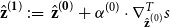 \begin{equation} \hat{\boldsymbol{z}}^{(\textbf{1})} \,:\!=\, \hat{\boldsymbol{z}}^{(\textbf{0})} + \alpha ^{(0)} \cdot \nabla ^T_{\hat{\boldsymbol{z}}^{(0)}} s \end{equation}
where $\alpha ^{(0)}$
is a (potentially dynamic) step width and
$\alpha ^{(0)}$
is a (potentially dynamic) step width and $\hat{\boldsymbol{z}}^{(\textbf{1})}$
again constitutes the subsequent first moment of the next iteration (see Fig. 2(c)).
$\hat{\boldsymbol{z}}^{(\textbf{1})}$
again constitutes the subsequent first moment of the next iteration (see Fig. 2(c)).
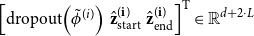
Iteration. Iterative application of the dialectical and the speculative moment’s formalizations yield a sequence of logits $\Big(\hat{\boldsymbol{z}}^{(\boldsymbol{k})}\Big)_{k=0}^{N}$
and predictions
$\Big(\hat{\boldsymbol{z}}^{(\boldsymbol{k})}\Big)_{k=0}^{N}$
and predictions $\Big(\hat{\boldsymbol{y}}^{(\boldsymbol{k})}\Big)_{k=0}^{N}$
where
$\Big(\hat{\boldsymbol{y}}^{(\boldsymbol{k})}\Big)_{k=0}^{N}$
where $k$
iterates between the initial prediction for
$k$
iterates between the initial prediction for $k=0$
and the ultimate prediction for
$k=0$
and the ultimate prediction for $k=N$
by applying
$k=N$
by applying $N$
gradient updates resulting from Equation (1).
$N$
gradient updates resulting from Equation (1).
In the following, we present a concrete implementation of this abstract formalization, focusing on the QA domain.
2.3 Implementation on Transformers for QA
Fig. 2 visualizes our formalization around the QA example introduced in Fig. 1. We now discuss QA-related implementation details.
2.3.1 Choosing parameters and functions
To apply our abstract thought flow method to a concrete model architecture, we have to (a) determine how we structure the model prediction logit vector $\hat{\boldsymbol{z}}$
; (b) choose an input representation
$\hat{\boldsymbol{z}}$
; (b) choose an input representation $\phi (\boldsymbol{x})$
(that is passed to
$\phi (\boldsymbol{x})$
(that is passed to $f_{\text{pred}}$
as well as
$f_{\text{pred}}$
as well as $f_{\text{corr}}$
); (c) choose a parametrization of the self-estimated correctness score prediction function
$f_{\text{corr}}$
); (c) choose a parametrization of the self-estimated correctness score prediction function $f_{\text{corr}}$
; and (d) define what the score
$f_{\text{corr}}$
; and (d) define what the score $s$
measures. In the following, we describe how these aspects can be realized in a Transformer-based QA model.
$s$
measures. In the following, we describe how these aspects can be realized in a Transformer-based QA model.
Composing $\hat{\boldsymbol{z}}$
. In extractive QA, a typical approach to answer span extraction from a context of
$\hat{\boldsymbol{z}}$
. In extractive QA, a typical approach to answer span extraction from a context of $L$
tokens is to use two probability distributions: (i)
$L$
tokens is to use two probability distributions: (i) $\hat{\boldsymbol{y}}_{\text{start}} \in [0,1]^L$
that assigns to each token a probability of starting the answer span, and (ii) a respective end token distribution
$\hat{\boldsymbol{y}}_{\text{start}} \in [0,1]^L$
that assigns to each token a probability of starting the answer span, and (ii) a respective end token distribution $\hat{\boldsymbol{y}}_{\text{end}} \in [0,1]^L$
for the probability of ending the answer span. To match our previously defined formalization, we define
$\hat{\boldsymbol{y}}_{\text{end}} \in [0,1]^L$
for the probability of ending the answer span. To match our previously defined formalization, we define $\hat{\boldsymbol{z}}^{(\boldsymbol{i})} \,:\!=\, \begin{bmatrix}\hat{\boldsymbol{z}}_{\text{start}}^{(\boldsymbol{i})} & {\hat{\boldsymbol{z}}_{\text{end}}^{(\boldsymbol{i})}}\end{bmatrix}^{\text{T}}$
which is linked to the corresponding probability distributions via the softmax function
$\hat{\boldsymbol{z}}^{(\boldsymbol{i})} \,:\!=\, \begin{bmatrix}\hat{\boldsymbol{z}}_{\text{start}}^{(\boldsymbol{i})} & {\hat{\boldsymbol{z}}_{\text{end}}^{(\boldsymbol{i})}}\end{bmatrix}^{\text{T}}$
which is linked to the corresponding probability distributions via the softmax function $\sigma$
:
$\sigma$
:
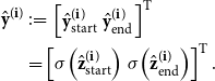 \begin{align*} \hat{\boldsymbol{y}}^{(\boldsymbol{i})} &\,:\!=\, \begin{bmatrix}\hat{\boldsymbol{y}}_{\text{start}}^{(\boldsymbol{i})} & {\hat{\boldsymbol{y}}_{\text{end}}^{(\boldsymbol{i})}}\end{bmatrix}^{\text{T}}\\ &= \begin{bmatrix}\sigma \!\left(\hat{\boldsymbol{z}}_{\text{start}}^{(\boldsymbol{i})}\right) & \sigma \!\left({\hat{\boldsymbol{z}}_{\text{end}}^{(\boldsymbol{i})}}\right)\end{bmatrix}^{\text{T}}. \end{align*}
Input Representation $\phi (\boldsymbol{x})$
. In contrast to Transformer-based classification models that conventionally rely on the embedding of the [CLS] token, typical Transformer-based QA models apply a linear function on top of each token’s embedding that maps the embedding to a start and an end logit. We follow this convention and define
$\phi (\boldsymbol{x})$
. In contrast to Transformer-based classification models that conventionally rely on the embedding of the [CLS] token, typical Transformer-based QA models apply a linear function on top of each token’s embedding that maps the embedding to a start and an end logit. We follow this convention and define
 \begin{align} \phi (\boldsymbol{x})& \,:\!=\, \left [ \mathbf{e_1}, \mathbf{e_2}, \ldots, \mathbf{e_{L}} \right ] \in \mathbb{R}^{d \times L} \end{align}
that is, as the sequence of $L$
contextualized embeddings with embedding dimension
$L$
contextualized embeddings with embedding dimension $d$
.
$d$
.
Choosing $f_{\text{corr}}$
. To represent the input within
$f_{\text{corr}}$
. To represent the input within $f_{\text{corr}}$
, we need a representation of
$f_{\text{corr}}$
, we need a representation of $\phi (\mathbf{x})$
that focuses on the relevant parts of the (potentially very long) input that were relevant to predict the start and end logits. We thus choose a weighted average over all token embeddings to retain as much as possible of the important information from the input while heavily reducing its available representation dimensionality to a single vector. As weights, we choose the element-wise product of the predicted start and end probabilities. We thus define a modified input encoding
$\phi (\mathbf{x})$
that focuses on the relevant parts of the (potentially very long) input that were relevant to predict the start and end logits. We thus choose a weighted average over all token embeddings to retain as much as possible of the important information from the input while heavily reducing its available representation dimensionality to a single vector. As weights, we choose the element-wise product of the predicted start and end probabilities. We thus define a modified input encoding $\tilde{\phi }^{(i)}(\mathbf{x}) \in \mathbb{R}^d$
where
$\tilde{\phi }^{(i)}(\mathbf{x}) \in \mathbb{R}^d$
where $d$
denotes the dimension of the embeddingsFootnote h as follows:
$d$
denotes the dimension of the embeddingsFootnote h as follows:
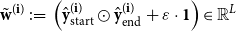 \begin{align} {\tilde{\boldsymbol{w}}^{(\boldsymbol{i})}} \,:\!=\, \left ( \hat{\boldsymbol{y}}_{\text{start}}^{(\boldsymbol{i})} \odot {\hat{\boldsymbol{y}}_{\text{end}}^{(\boldsymbol{i})}} + \varepsilon \cdot \mathbf{1} \right ) & \in \mathbb{R}^{L} \end{align}
 \begin{align} \tilde{\phi }(\mathbf{x})^{(i)} \,:\!=\, \phi (\mathbf{x}) \cdot \frac{{\tilde{\boldsymbol{w}}^{(\boldsymbol{i})}}}{\Sigma _j {\tilde{\boldsymbol{w}}^{(\boldsymbol{i})}}_j} & \in \mathbb{R}^d\qquad \qquad\quad\end{align}
where $\varepsilon$
is a small constant that ensures that we do not divide by zero,
$\varepsilon$
is a small constant that ensures that we do not divide by zero, $e_i$
is the embedding of the
$e_i$
is the embedding of the $i$
-th token,
$i$
-th token, $\odot$
is element-wise multiplication, and
$\odot$
is element-wise multiplication, and $L$
is the maximum number of tokens in the context. This modified input representation
$L$
is the maximum number of tokens in the context. This modified input representation $\tilde{\phi }(\mathbf{x})^{(i)}$
can be regarded to be a dynamic perspective onto
$\tilde{\phi }(\mathbf{x})^{(i)}$
can be regarded to be a dynamic perspective onto $\phi (\mathbf{x})$
that highlights these parts of
$\phi (\mathbf{x})$
that highlights these parts of $\phi (\boldsymbol{x})$
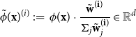
that are most important to the model’s answer prediction. The intuition behind this is that the correction module should have access to all information about the context that the prediction model focused on. Based on initial empirical findings, we choose to use a two-layer multi-layer perceptron (MLP) with scaled exponential linear unit (SELU) activation (Klambauer et al. Reference Klambauer, Unterthiner, Mayr and Hochreiter2017) to map the concatenated vector
$\phi (\boldsymbol{x})$
that are most important to the model’s answer prediction. The intuition behind this is that the correction module should have access to all information about the context that the prediction model focused on. Based on initial empirical findings, we choose to use a two-layer multi-layer perceptron (MLP) with scaled exponential linear unit (SELU) activation (Klambauer et al. Reference Klambauer, Unterthiner, Mayr and Hochreiter2017) to map the concatenated vector
 \begin{equation} \begin{bmatrix}\text{dropout}\!\left(\tilde{\phi }^{(i)}\right) & {\hat{\boldsymbol{z}}^{(\boldsymbol{i})}_{\text{start}}} & {\hat{\boldsymbol{z}}^{(\boldsymbol{i})}_{\text{end}}}\end{bmatrix}^{\text{T}} \in \mathbb{R}^{d+2\cdot L} \end{equation}
to an estimated correctness score $s$
. Note that
$s$
. Note that $f_{\text{corr}}$
does not receive the decoded answer text but uses the start and end logits directly to provide differentiability.
$f_{\text{corr}}$
does not receive the decoded answer text but uses the start and end logits directly to provide differentiability.
Correctness Score $s$
. Following standard evaluation metrics for QA, we use the
$s$
. Following standard evaluation metrics for QA, we use the $\text{F}_1$
-score of the predicted answer as the correctness score target that
$\text{F}_1$
-score of the predicted answer as the correctness score target that $f_{\text{corr}}$
is trained to predict.
$f_{\text{corr}}$
is trained to predict.
2.3.2 Training
To train $f_{\text{corr}}$
, we freeze the parameters of
$f_{\text{corr}}$
, we freeze the parameters of $f_{\text{pred}}$
. Then, we pass the training instances through the whole model (including
$f_{\text{pred}}$
. Then, we pass the training instances through the whole model (including $\phi$
,
$\phi$
, $f_{\text{pred}}$
, and
$f_{\text{pred}}$
, and $f_{\text{corr}}$
) as shown in Fig. 2(a) to obtain the target of the predicted correctness score
$f_{\text{corr}}$
) as shown in Fig. 2(a) to obtain the target of the predicted correctness score $s$
. We determine the ground-truth correctness score by calculating the
$s$
. We determine the ground-truth correctness score by calculating the $\text{F}_1$
-score between the ground-truth answer and the answer prediction from
$\text{F}_1$
-score between the ground-truth answer and the answer prediction from $f_{\text{pred}}$
. We define the correctness estimate prediction loss as the mean squared error between the calculated score, and the predicted
$f_{\text{pred}}$
. We define the correctness estimate prediction loss as the mean squared error between the calculated score, and the predicted $s$
and train
$s$
and train $f_{\text{corr}}$
to minimize it. Overall, we thus train
$f_{\text{corr}}$
to minimize it. Overall, we thus train $f_{\text{corr}}$
to score how correct a model prediction (represented by the start and end logits) is given a model input (represented by the condensed input encoding
$f_{\text{corr}}$
to score how correct a model prediction (represented by the start and end logits) is given a model input (represented by the condensed input encoding $\tilde{\phi }(\mathbf{x})$
) and use the model’s predictions on the training set to generate ground-truth correctness scores (using
$\tilde{\phi }(\mathbf{x})$
) and use the model’s predictions on the training set to generate ground-truth correctness scores (using $\text{F}_1$
-score).
$\text{F}_1$
-score).
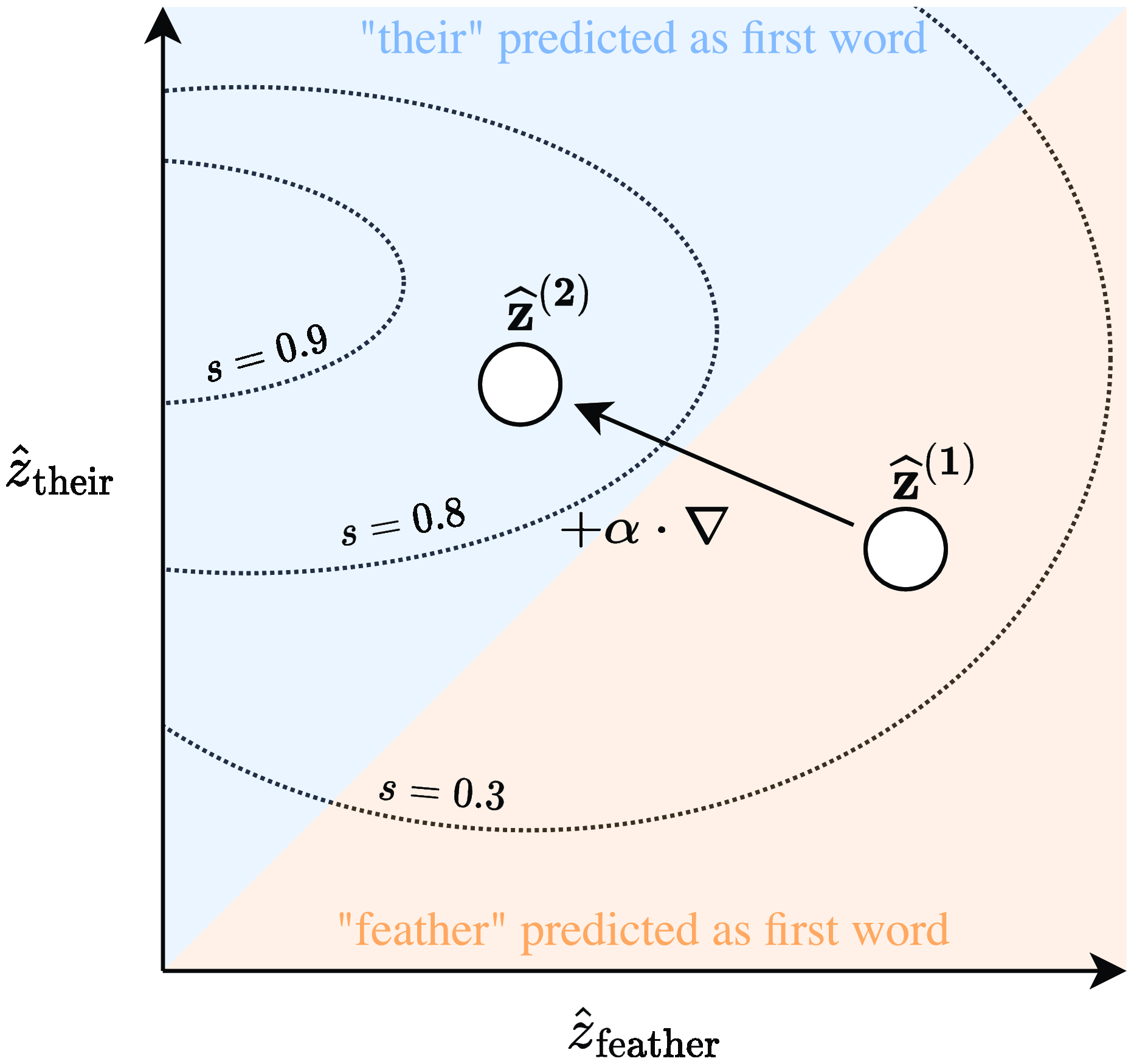
Figure 3. Simplified visualization of the modification step (during inference) shown in Fig. 2 depicted within a cut through the logits space. The axes correspond to the elements of ${\hat{\boldsymbol{z}}_{\text{start}}}$
that represent the index positions of the words “feather” and “their” as shown in the example in Fig. 1. The dotted isolines correspond to the self-estimated correctness scores obtained from
${\hat{\boldsymbol{z}}_{\text{start}}}$
that represent the index positions of the words “feather” and “their” as shown in the example in Fig. 1. The dotted isolines correspond to the self-estimated correctness scores obtained from $f_{\text{corr}}$
. Before the modification, the system’s prediction corresponding to
$f_{\text{corr}}$
. Before the modification, the system’s prediction corresponding to $\hat{\boldsymbol{z}}^{(\textbf{1})}$
would be an answer starting at “feather.” The gradient
$\hat{\boldsymbol{z}}^{(\textbf{1})}$
would be an answer starting at “feather.” The gradient $\nabla$
points in the direction of an improvement of self-estimated correctness of
$\nabla$
points in the direction of an improvement of self-estimated correctness of $\hat{\boldsymbol{z}}^{(\textbf{1})}$
. After a gradient step into the direction of
$\hat{\boldsymbol{z}}^{(\textbf{1})}$
. After a gradient step into the direction of $\nabla$
, the change in logits towards
$\nabla$
, the change in logits towards ${\hat{\boldsymbol{z}}^{(2)}}$
leads to a shift of the answer start position. The modification behavior emerges solely from the logit modifications and can lead to complex modification patterns (see Section 3.3).
${\hat{\boldsymbol{z}}^{(2)}}$
leads to a shift of the answer start position. The modification behavior emerges solely from the logit modifications and can lead to complex modification patterns (see Section 3.3).
2.3.3 Inference
At inference time, we encode a new input and predict (i) the answer start and end logits using $f_{\text{pred}}$
and (ii) an estimated
$f_{\text{pred}}$
and (ii) an estimated $\text{F}_1$
-score
$\text{F}_1$
-score $s$
of the predicted answer span using the correction module
$s$
of the predicted answer span using the correction module $f_{\text{corr}}$
as shown in Fig. 2(a). Instead of directly using the initial logits as the model’s prediction—as would be done in a standard model—we iteratively update the logits with respect to the estimated correctness score’s gradient following our formalization from Section 2.2 as shown in Fig. 2(b),(c). Fig. 3 depicts a simplified visualization of one gradient update that changes the model’s prediction.
$f_{\text{corr}}$
as shown in Fig. 2(a). Instead of directly using the initial logits as the model’s prediction—as would be done in a standard model—we iteratively update the logits with respect to the estimated correctness score’s gradient following our formalization from Section 2.2 as shown in Fig. 2(b),(c). Fig. 3 depicts a simplified visualization of one gradient update that changes the model’s prediction.
Update Rule. As described in Section 2.2, we aim at modifying $\hat{\boldsymbol{z}}^{(i)}$
so that the correction module assigns an increased correctness (i.e.,
$\hat{\boldsymbol{z}}^{(i)}$
so that the correction module assigns an increased correctness (i.e., $\text{F}_1$
-score in our QA application). To apply Equation (1), we have to define how the step size
$\text{F}_1$
-score in our QA application). To apply Equation (1), we have to define how the step size $\alpha$
is chosen in our QA application. We choose
$\alpha$
is chosen in our QA application. We choose $\alpha$
such that a predefined probability mass
$\alpha$
such that a predefined probability mass $\delta$
is expected to move. To this end, we first take a probing step of length one, calculate the distance as the
$\delta$
is expected to move. To this end, we first take a probing step of length one, calculate the distance as the $L_1$
norm between the initial distribution and the probe distribution, and choose the step width
$L_1$
norm between the initial distribution and the probe distribution, and choose the step width $\alpha \in \mathbb{R}^+$
such that it scales the linearized
$\alpha \in \mathbb{R}^+$
such that it scales the linearized $L_1$
distance to the hyperparameter
$L_1$
distance to the hyperparameter $\delta$
as follows:
$\delta$
as follows:
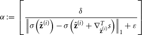 \begin{equation} \alpha \,:\!=\, \left [\frac{\delta }{\left\|\sigma \!\left(\hat{\boldsymbol{z}}^{(i)}\right) - \sigma \!\left(\hat{\boldsymbol{z}}^{(i)} + \nabla ^T_{\hat{\boldsymbol{z}}^{(i)}} s\right)\right\|_1 + \varepsilon } \right ] \end{equation}
where $\sigma ({\cdot})$
denotes the softmax function,
$\sigma ({\cdot})$
denotes the softmax function, $s$
is the correctness score as defined above, and
$s$
is the correctness score as defined above, and $\varepsilon \in \mathbb{R^+}$
is a small constant for numerical stability.
$\varepsilon \in \mathbb{R^+}$
is a small constant for numerical stability.
Monte Carlo Dropout Stabilization. The gradient $\nabla _{\hat{\boldsymbol{z}}^{(i)}} s$
is deterministic but it can, as we found in our preliminary experiments, be sensitive to small changes in the input representation
$\nabla _{\hat{\boldsymbol{z}}^{(i)}} s$
is deterministic but it can, as we found in our preliminary experiments, be sensitive to small changes in the input representation $\phi (\mathbf{x})$
. We therefore stabilize our correction gradient estimation by sampling and averaging gradients instead. For this, we use the dropped-out input encoding from Equation (5) and sample five gradients for every step using MCDrop (Gal and Ghahramani Reference Gal and Ghahramani2016).
$\phi (\mathbf{x})$
. We therefore stabilize our correction gradient estimation by sampling and averaging gradients instead. For this, we use the dropped-out input encoding from Equation (5) and sample five gradients for every step using MCDrop (Gal and Ghahramani Reference Gal and Ghahramani2016).
3. Question answering experiments
3.1 Data, model, and training
3.1.1 Data set
We choose the HotpotQA data set (distractor setting) (Yang et al. Reference Yang, Qi, Zhang, Bengio, Cohen, Salakhutdinov and Manning2018) to evaluate our models because it contains complex questions that require multi-hop reasoning over two Wikipedia articles. In the distractor setting, the model is “distracted” by eight irrelevant articles which are passed to the model alongside a pair of relevant articles. In addition to yes/no/answer span annotations, HotpotQA also provides explanation annotations in the form of binary relevance labels over the paragraphs of the relevant articles which we do not use when training our models. As the public test set is undisclosed, we use the official validation set as our test set and a custom validation set with 10k instances sampled from the training set leaving 80,564 instances for training.
3.1.2 Base model
Our underlying QA model is Longformer-largeFootnote i (Beltagy, Peters, and Cohan Reference Beltagy, Peters and Cohan2020) with a final linear layer that maps token embeddings to start and end logits. The model reaches 63.5% $\text{F}_1$
(SD = 0.6) on the HotpotQA validation set averaged over three random seeds and can handle input lengths of up to 4096 tokens which enables us to feed in the entire context as a single instance without truncation. The model’s input is a single token sequence that contains the question followed by the answer context (i.e., the concatenation of 8 + 2 Wikipedia articles). The model outputs two distributions over the input tokens (i.e., two 4096-dimensional distributions), namely (a) one for the answer start position and (b) another for the answer end position, respectively. In this commonly used extractive QA setting, the model can choose its answer from any text span within the context. We prepend a “yes” and a “no” token to the context (instead of adding a categorical prediction head for these answer options) because doing so makes it easier to align distributions across answer options and text span options. In total, this model has 435 M parameters of which only 331k parameters are added by our MLP implementation of
$\text{F}_1$
(SD = 0.6) on the HotpotQA validation set averaged over three random seeds and can handle input lengths of up to 4096 tokens which enables us to feed in the entire context as a single instance without truncation. The model’s input is a single token sequence that contains the question followed by the answer context (i.e., the concatenation of 8 + 2 Wikipedia articles). The model outputs two distributions over the input tokens (i.e., two 4096-dimensional distributions), namely (a) one for the answer start position and (b) another for the answer end position, respectively. In this commonly used extractive QA setting, the model can choose its answer from any text span within the context. We prepend a “yes” and a “no” token to the context (instead of adding a categorical prediction head for these answer options) because doing so makes it easier to align distributions across answer options and text span options. In total, this model has 435 M parameters of which only 331k parameters are added by our MLP implementation of $f_{\text{corr}}$
.
$f_{\text{corr}}$
.
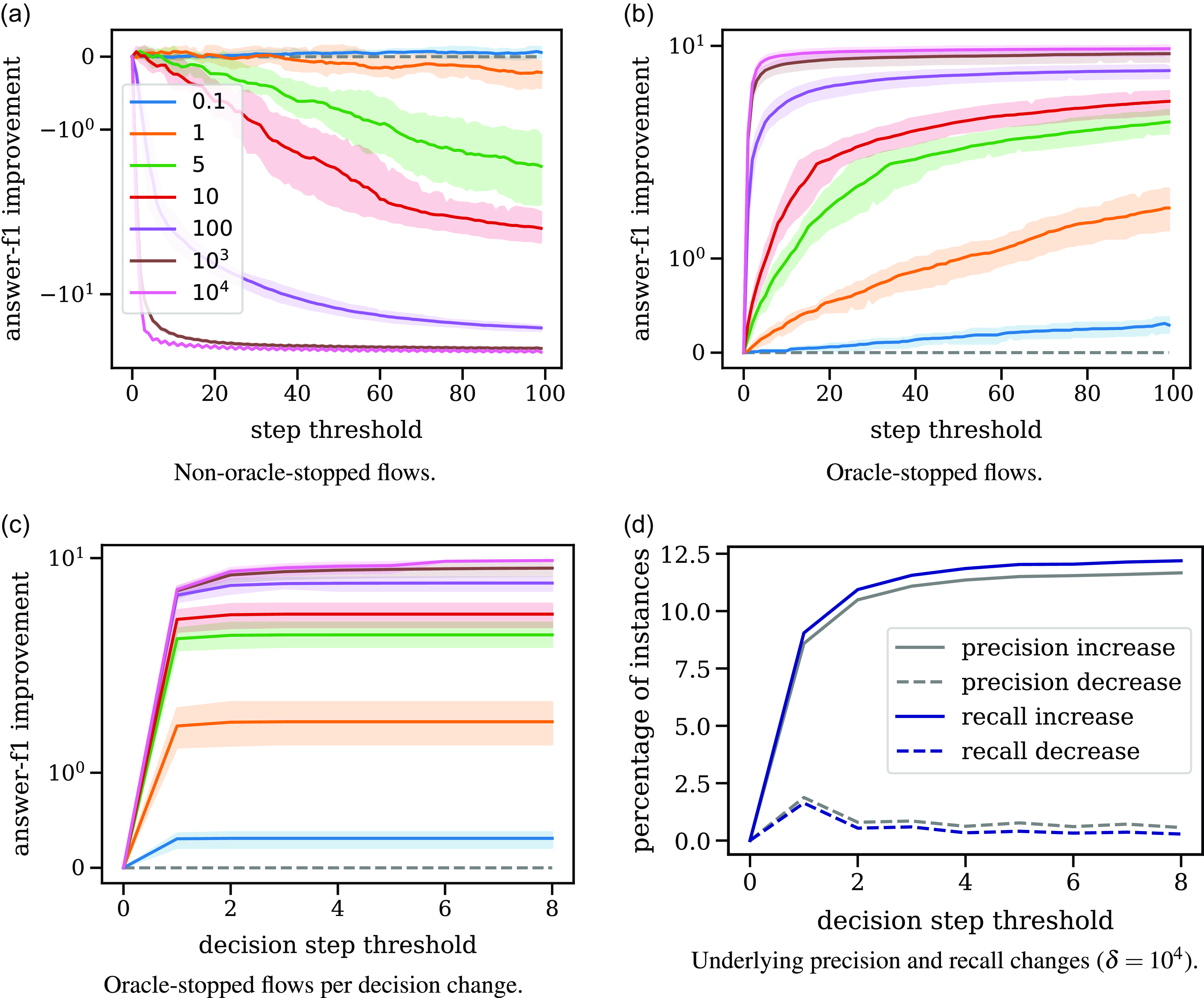
Figure 4. Thought flows with different gradient scaling targets $\delta$
averaged over three seeds of a QA model. Higher values for
$\delta$
averaged over three seeds of a QA model. Higher values for $\delta$
correspond to more aggressive decision changes. Without a stopping oracle that stops when the thought flow no longer improves an answer (top left), only
$\delta$
correspond to more aggressive decision changes. Without a stopping oracle that stops when the thought flow no longer improves an answer (top left), only $\delta =0.1$
provides consistently stable, but very small
$\delta =0.1$
provides consistently stable, but very small $\text{F}_1$
improvements. With an oracle (top right), higher values for
$\text{F}_1$
improvements. With an oracle (top right), higher values for $\delta$
reach higher and faster
$\delta$
reach higher and faster $\text{F}_1$
improvements up to
$\text{F}_1$
improvements up to $\gt$
9%. Nearly all performance gains are achieved by the first decision change (bottom left). A detailed analysis of flows using
$\gt$
9%. Nearly all performance gains are achieved by the first decision change (bottom left). A detailed analysis of flows using $\delta =10^4$
shows that the observed
$\delta =10^4$
shows that the observed $\text{F}_1$
improvements are the result of slight decreases and stronger increases in both precision and recall (bottom right). y axes of plots (a), (b), and (c) use a symlog scale. Improvements are reported as absolute
$\text{F}_1$
improvements are the result of slight decreases and stronger increases in both precision and recall (bottom right). y axes of plots (a), (b), and (c) use a symlog scale. Improvements are reported as absolute $\text{F}_1$
score differences to the base model performance of 63.5%
$\text{F}_1$
score differences to the base model performance of 63.5% $\text{F}_1$
.
$\text{F}_1$
.
3.1.3 Training details
We first train the base models for five epochs on a single V100 GPU using a learning rate of $10^{-5}$
, an effective batch size of 64, an AdamW optimizer (Loshchilov and Hutter Reference Loshchilov and Hutter2019), early stopping, and a cross-entropy loss on the start/end logits. We subsequently train the correction modules using the same setting but with the mean squared error loss function for
$10^{-5}$
, an effective batch size of 64, an AdamW optimizer (Loshchilov and Hutter Reference Loshchilov and Hutter2019), early stopping, and a cross-entropy loss on the start/end logits. We subsequently train the correction modules using the same setting but with the mean squared error loss function for $\text{F}_1$
-score prediction training. Training a single model each took approximately three days. In the following, we report all results as averages over three random seeds including standard deviations.
$\text{F}_1$
-score prediction training. Training a single model each took approximately three days. In the following, we report all results as averages over three random seeds including standard deviations.
3.2 Performance improvements
3.2.1 Performance over steps
Fig. 4(a) shows how $\text{F}_1$
-scores per gradient scaling target
$\text{F}_1$
-scores per gradient scaling target $\delta$
evolve over 100 steps. We observe that small
$\delta$
evolve over 100 steps. We observe that small $\delta$
values lead to small
$\delta$
values lead to small $\text{F}_1$
improvements. While
$\text{F}_1$
improvements. While $\delta =0.1$
consistently improves
$\delta =0.1$
consistently improves $\text{F}_1$
-scores, all other
$\text{F}_1$
-scores, all other $\delta$
values eventually deteriorate
$\delta$
values eventually deteriorate $\text{F}_1$
-scores. The higher the
$\text{F}_1$
-scores. The higher the $\delta$
value, the faster the
$\delta$
value, the faster the $\text{F}_1$
decrease. We conclude that (i) very small
$\text{F}_1$
decrease. We conclude that (i) very small $\delta$
values fail to offer notable performance gains and that (ii) a larger
$\delta$
values fail to offer notable performance gains and that (ii) a larger $\delta$
can improve performance at the beginning but then “overshoot” with their corrections. We hypothesize that a remedy to this tradeoff is to use larger
$\delta$
can improve performance at the beginning but then “overshoot” with their corrections. We hypothesize that a remedy to this tradeoff is to use larger $\delta$
values but stop the modification process at the right time.
$\delta$
values but stop the modification process at the right time.
3.2.2 Stopping via an oracle
To test the hypothesis that stopping modifications at the right time can unlock notable performance improvements, we introduce a stopping function which uses an oracle to stop the thought flow when the best $\text{F}_1$
performance level is detected. Fig. 4(b) shows that, with this oracle function, thought flows can reach performance improvements of up to 9.6%
$\text{F}_1$
performance level is detected. Fig. 4(b) shows that, with this oracle function, thought flows can reach performance improvements of up to 9.6% $\text{F}_1$
(SD = 0.61) corresponding to an absolute best average performance of 73.1%
$\text{F}_1$
(SD = 0.61) corresponding to an absolute best average performance of 73.1% $\text{F}_1$
using
$\text{F}_1$
using $\delta =10^4$
.
$\delta =10^4$
.
Fig. 4(c) shows that almost all performance improvements are due to the first decision change within the thought flows. Moreover, answer spans improve constantly and do not randomly shift across the context. This observation suggests that singular thought flow changes are highly effective and can make substantial corrections rapidly.
Fig. 4(d) shows that the observed $\text{F}_1$
improvements are the result of an overall increase in precision and recall. In turn, these increases are composed of small decreases in precision and recall that are outweighed by stronger increases across all decision step thresholds. Fig. 4(d) displays the fraction of instances for which precision/recall values decrease/increase for thought flows with
$\text{F}_1$
improvements are the result of an overall increase in precision and recall. In turn, these increases are composed of small decreases in precision and recall that are outweighed by stronger increases across all decision step thresholds. Fig. 4(d) displays the fraction of instances for which precision/recall values decrease/increase for thought flows with $\delta = 10^4$
. We provide the respective analyses for additional
$\delta = 10^4$
. We provide the respective analyses for additional $\delta$
values in Figure B1 in Appendix B.2.
$\delta$
values in Figure B1 in Appendix B.2.
3.3 Thought flow patterns
In the following, we investigate which answer span modifications lead to the observed performance improvements. Note that we did not manually specify or limit the possible answer span modification types. Instead, all observed modification patterns emerge solely based on changes in the underlying start and end position distributions, and these changes are induced by gradient steps in the direction of improved self-estimated prediction correctness.
Table 2. Emergent thought flow modification patterns identified in 150 randomly sampled thought flows using $\delta =1$
. The correct answer is marked in bold, and the predicted answer per flow step is marked in orange
$\delta =1$
. The correct answer is marked in bold, and the predicted answer per flow step is marked in orange
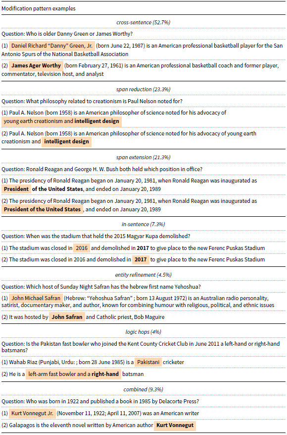
We randomly sample 150 instances from the subset of the official validation split for which the thought flow changed the initial answer prediction. We identify six (non-exclusive) basic modification patterns as well as two additional composed modification patterns that all emerge from the combination of correctness self-estimation and iterative prediction updates and show selected examples in Table 2. We provide additional examples for each correction pattern in Table B1. Further, Table 3 shows additional thought flow examples using three modification steps.
Cross-Sentence. With 52.7%, this is the most frequent type of modification pattern. The thought flow moves the predicted answer span from one sentence to another.
Span Reduction. The thought flow can shorten the predicted span to modify the answer.
Span Extension. Similarly, the thought flow can also expand a predicted answer span to modify it.
In-Sentence. Beyond in-sentence span reduction/extension, the thought flow can also shift between non-overlapping spans within a sentence.
Entity Refinement. In this modification pattern, the thought flow keeps predicting the same entity but switches the predicted answer to an alternative mention of the entity.
Logic Hops. The thought flow performs a step-wise reasoning that first resolves the first step of a two-step reasoning structure before jumping to the second step, that is the modified answer.
Combinations. We observe various combinations of the aforementioned patterns. A model can, for instance, jump between sentences, refine entities, and reduce the answer span.
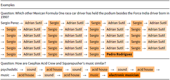
Sequential Modifications. Modifications can also occur sequentially as shown in the examples in Table 3. While the example in the upper part of Table 3 demonstrates a combination of a cross-sentence modification followed by a span reduction modification, the example in the lower part illustrates how a span extension modification can iteratively improve a prediction. We additionally observe flow patterns with very high numbers of answer modifications. These typically correspond to sequences of modifications in which the answer periodically alternates between two or three answer alternatives or in which the change of answers exhibits seemingly chaotic behavior. Table 4 shows two example flows that contain 45 and 12 decision changes. The first example shows a frequently observed long-flow modification pattern in which the initial decision is followed by a 2-cycle between two alternative decisions before the answer changes to the final answer that was not predicted before.
Table 3. Multi-step modification examples ( $\delta =1$
). The correct answer is marked in bold, the predicted answer per flow step is marked in orange
$\delta =1$
). The correct answer is marked in bold, the predicted answer per flow step is marked in orange
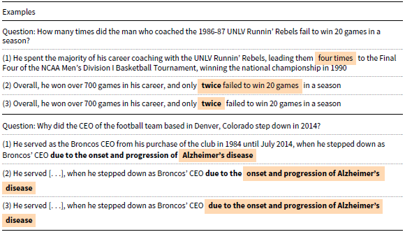
Table 4. Examples of long thought flows. The table shows two questions for which the resulting thought flow contains 45 prediction changes and 12 decision changes respectively. In contrast to previous tables, the answer contexts are omitted and only the predicted answer spans are displayed. Different shades of orange background reflect repeated answer spans and highlights, for example, a 2-cycle for the first example
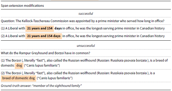
While the previous examples showed thought flow modifications that result in a successful modification of a wrong or incomplete answer to the correct answer, thought flow modifications can also deteriorate answer correctness. We provide comparisons of successful and unsuccessful modifications for two frequent modification patterns (i.e., cross-sentence and span extension modifications) in Table 5 and Table 6. Overall, we do not observe a systematic correspondence between successful/unsuccessful modification and specific modification pattern types or question characteristics. We provide additional examples of the discussed modification patterns in Appendix B.2.
Table 5. Examples of successful (incorrect $\rightarrow$
correct) and unsuccessful cross-sentence modifications. The correct answer is marked in bold, and the predicted answer per flow step is marked in orange
$\rightarrow$
correct) and unsuccessful cross-sentence modifications. The correct answer is marked in bold, and the predicted answer per flow step is marked in orange
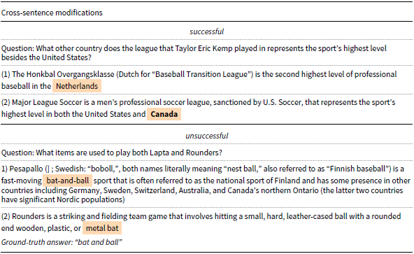
Table 6. Examples of successful (incorrect $\rightarrow$
correct) and unsuccessful span extension modifications. The correct answer is marked in bold, and the predicted answer per flow step is marked in orange
$\rightarrow$
correct) and unsuccessful span extension modifications. The correct answer is marked in bold, and the predicted answer per flow step is marked in orange
4. Human evaluation
While the previous section showed that thought flows can yield complex prediction modification patterns and can reach promising performance gains, we now investigate how thought flow predictions affect human users in an AI-assisted QA task.
4.1 Experiment design
We choose a within-subject design in which each participant is exposed to three variations of a QA system.
4.1.1 Conditions
We aim to assess the effect of the thought flow concept on users and therefore present the outputs of the oracle-stopped thought flow in one condition (TF) and compare it to two baseline conditions. As baselines, we use top-1 predictions ( single ) (to compare against standard models) and top-3 predictions ( top-3) (to compare to an alternative approach to show several predictions). For all conditions, we present the predicted answer(s) along with the sentence in which they appear in the context.
4.1.2 Dependent variables
We study the effect of the condition (single, TF, and top-3) on a set of dependent variables. We include variables on a per-question level (after each question) and on a per-system level (after all questions of one condition).
The per-question variables include the following: (i) human answer correctness, (ii) perceived model correctness, (iii) perceived understanding, (iv) perceived helpfulness, and (v) completion time. The per-system variables include: (vi) usability using the Usability Metric for User Experience (UMUX) questionnaire (Finstad Reference Finstad2010, Reference Finstad2013), (vii) mental effort using the Paas scale (Paas Reference Paas1992), (viii) anthropomorphism using the respective subscale of the Godspeed questionnaire (Bartneck et al. Reference Bartneck, Kulic, Croft and Zoghbi2009), (ix) perceived intelligence using the subscale from the same questionnaire, and (x) average completion time.Footnote j We provide a list of all questionnaires in the appendix.
4.1.3 Apparatus
We sample 100 instances from the HotpotQA validation instances in which a thought flow using $\delta =1$
made at least one prediction change.Footnote k From these, we sample 30 instances per participant and randomly assign the instances to three bins of 10 questions (one bin per condition).Footnote l We balance the six possible condition orders across participants and include three attention checks per participant. Fig. 5 shows our user study interface for the TF condition in the example of the previously discussed thought flow instance. We provide screenshots of all conditions’ interfaces in the appendix.
$\delta =1$
made at least one prediction change.Footnote k From these, we sample 30 instances per participant and randomly assign the instances to three bins of 10 questions (one bin per condition).Footnote l We balance the six possible condition orders across participants and include three attention checks per participant. Fig. 5 shows our user study interface for the TF condition in the example of the previously discussed thought flow instance. We provide screenshots of all conditions’ interfaces in the appendix.
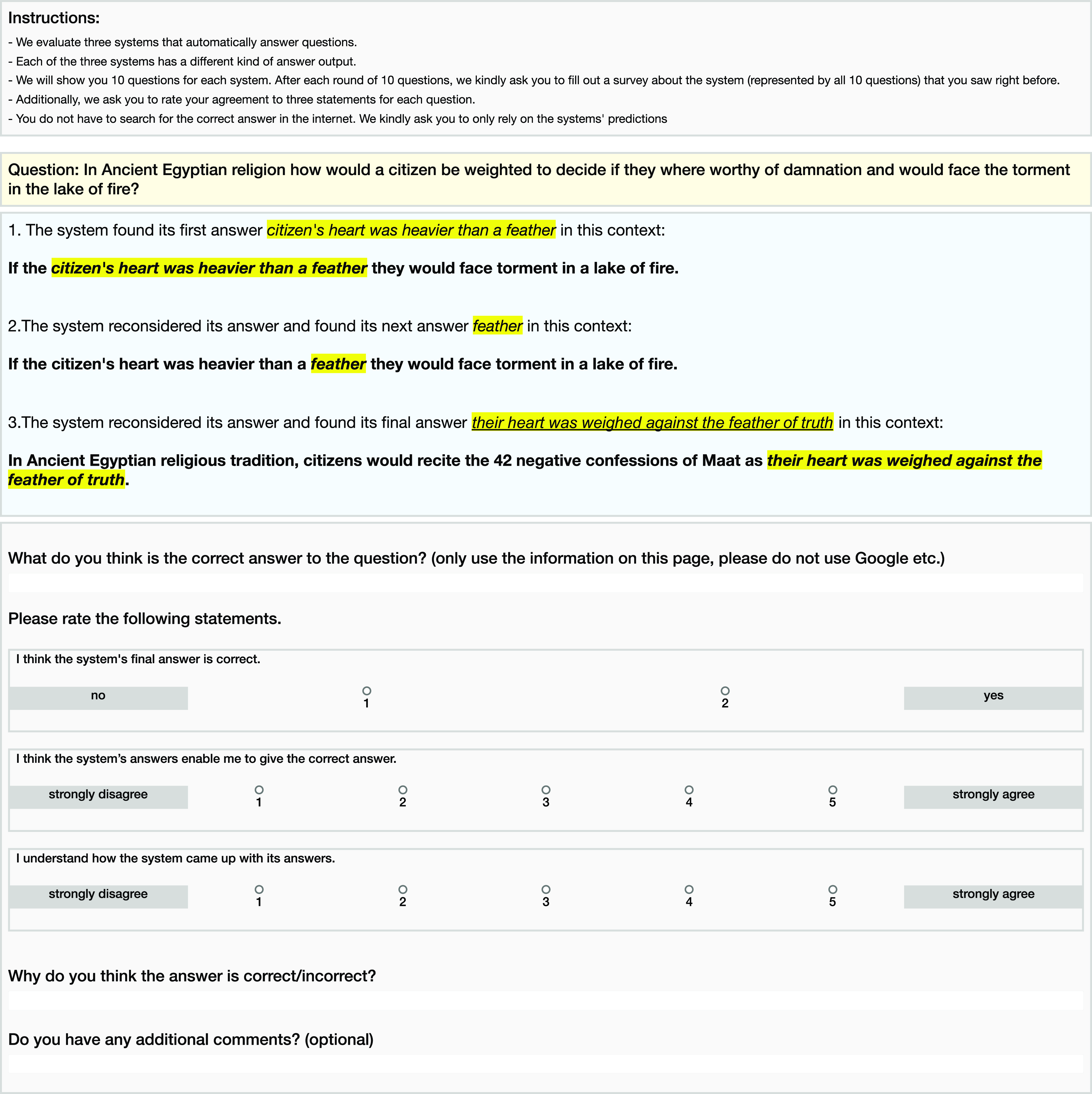
Figure 5. User study interface showing the TF condition (ours).
4.2 Quantitative results
We use MTurkFootnote m to recruit US-based crowdworkers with $\gt$
90% approval rate and the MTurk Masters qualification to be consistent with previous human evaluations of explainability on the HotpotQA data set (i.a., Schuff et al. Reference Schuff, Vanderlyn, Adel and Vu2023a). We collect responses from 55 workers.Footnote n
$\gt$
90% approval rate and the MTurk Masters qualification to be consistent with previous human evaluations of explainability on the HotpotQA data set (i.a., Schuff et al. Reference Schuff, Vanderlyn, Adel and Vu2023a). We collect responses from 55 workers.Footnote n
4.2.1 Statistical models
Per-System Ratings. To test for statistically significant effects of the choice of QA system (single answer, top-3, and thought flow) on the per-system ratings, we make use of Friedman tests (Pereira, Afonso, and Medeiros Reference Pereira, Afonso and Medeiros2015) to account for the paired responses induced by the within-subject design.Footnote o We use Holm-corrected Conover post hoc tests to identify significant pairwise differences.Footnote p
Per-Item Ratings. Note that the within-subject design of our study possibly introduces inter-dependencies within ratings that we have to account for using an appropriate statistical model. Additionally, our dependent variables are measured on different levels, for example completion time is measured on a ratio scale while human answer correctness is measured on a nominal (dichotomous) scale.Footnote q We, therefore, use (generalized) linear mixed models (GLMM) and cumulative link mixed models (CLMM) to (i) account for random effects of question and subject IDs, and (ii) account for the variables’ respective measurement scales.Footnote r We use Likelihood-ratio tests (LRT) between the full model and the model without the condition variable to identify main effects of the condition variable and conduct Holm-corrected Tukey post hoc tests.
Table 7. Statistical results of our human evaluation ( $N=55$
). “
$N=55$
). “ $^{*}$
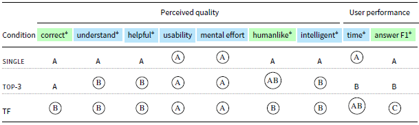
” marks dependent variables on which a significant effect of the system condition was observed (Friedman tests and LRT tests for GLMM/CLMM). Pairwise differences between conditions (Holm-adjusted Tukey/Conover tests) are reported as compact letter display codings. For example, the “human-like” column shows that the post hoc test detected a significant difference between single and TF but no significant difference between any other pair. Similarly, the last column shows pairwise differences between all conditions and the TF condition reaches significantly higher human answer
$^{*}$
” marks dependent variables on which a significant effect of the system condition was observed (Friedman tests and LRT tests for GLMM/CLMM). Pairwise differences between conditions (Holm-adjusted Tukey/Conover tests) are reported as compact letter display codings. For example, the “human-like” column shows that the post hoc test detected a significant difference between single and TF but no significant difference between any other pair. Similarly, the last column shows pairwise differences between all conditions and the TF condition reaches significantly higher human answer $\text{F}_1$
-scores than any other conditions. Variables for which TF is among the best-performing models are marked in cyan, variables for which it is found to be the sole superior system are marked in green
$\text{F}_1$
-scores than any other conditions. Variables for which TF is among the best-performing models are marked in cyan, variables for which it is found to be the sole superior system are marked in green


4.2.2 Results
We find significant differences for all dependent variables except usability and mental effort. We summarize the results of our statistical analysis in Table 7 using CLD codings (Piepho Reference Piepho2004). Table 8 provides the $p$
values for main effects and each pairwise comparison. In the following, we discuss our findings for each dependent variable for which we found a significant main effect.
$p$
values for main effects and each pairwise comparison. In the following, we discuss our findings for each dependent variable for which we found a significant main effect.
Perceived Answer Correctness. While there is no statistically significant difference between showing single answers or top-3 predictions to users, displaying thought flows leads to significantly higher answer correctness ratings.
Understanding. Top-3 as well as thought flow predictions significantly increased the subjectively perceived level of understanding of how the system came up with its answer compared to single predictions.
Helpfulness. Similarly, top-3 and the thought flow predictions significantly improve perceived system helpfulness compared to single predictions.
Anthropomorphism. While we observe no significant difference in anthropomorphism ratings between single and top-3 predictions, the thought flow predictions are perceived as significantly more human-like/natural than single answers.
Perceived intelligence. Both, top-3 and the thought flow predictions lead to significantly increased perceived system intelligence.
Completion Time. We observe that the top-3 predictions significantly improve completion times compared to single answers although there is no significant increase for thought flows.
User Performance. Compared to single answers, top-3 predictions already improve user performance in terms of $\text{F}_1$
-score of the answer which the user decided on using the system. However, thought flow predictions allow for even higher human-AI performances which are significantly higher than answers given in the single answer or top-3 conditions. We additionally analyze user answers using exact match scores and observe the same effects and model orders.
$\text{F}_1$
-score of the answer which the user decided on using the system. However, thought flow predictions allow for even higher human-AI performances which are significantly higher than answers given in the single answer or top-3 conditions. We additionally analyze user answers using exact match scores and observe the same effects and model orders.
Overall, our results indicate that thought flows are better than or as good as single answer or top-3 predictions across all dimensions evaluated. In particular for perceived answer correctness, humanlikeness, and user performance, thought flows are significantly better than both single answers and top-3 predictions. While comparable (statistically indistinguishable) improvements of understanding, helpfulness, naturalness, and intelligence can also be achieved using top-3 predictions, these come at the cost of significantly increased completion times compared to single answers. In contrast, we do not find a significant time increase using thought flows.
5. Application to other tasks and domains
So far, we explored our thought flow method in the context of QA systems. As our method only requires a model to provide a vector representation of the model input and a differentiably linked model output, it can be applied to the vast majority of, e.g., classification models within as well as outside NLP. In the following, we demonstrate an exemplary application to image classification.
We use a pre-trained vision Transformer model (Dosovitskiy et al. Reference Dosovitskiy, Beyer, Kolesnikov, Weissenborn, Zhai, Unterthiner, Dehghani, Minderer, Heigold, Gelly, Uszkoreit and Houlsby2020) as base model and fine-tune the model on the CIFAR-10 and CIFAR-100 image classification datasets (Krizhevsky Reference Krizhevsky2009). We use the ViT-L-32 model variant pre-trained on the ILSVRC-2012 ImageNet and the ImageNet-21k datasets (Deng et al. Reference Deng, Dong, Socher, Li, Li and Fei-Fei2009) as described by Dosovitskiy et al. (Reference Dosovitskiy, Beyer, Kolesnikov, Weissenborn, Zhai, Unterthiner, Dehghani, Minderer, Heigold, Gelly, Uszkoreit and Houlsby2020).Footnote s
As for our QA implementation discussed in Section 2.3, we have to specify our choice of logit vector $\hat{\boldsymbol{z}}$
, input representation
$\hat{\boldsymbol{z}}$
, input representation $\phi (\boldsymbol{x})$
, correctness score
$\phi (\boldsymbol{x})$
, correctness score $s$
, and correctness score prediction function
$s$
, and correctness score prediction function $f_{\text{corr}}$
. While our QA span extraction model did yield two probability distributions (one for the start position and one for the end position), we now only have to consider a single distribution over image classes. Following our notation in Section 2.3, we thus define
$f_{\text{corr}}$
. While our QA span extraction model did yield two probability distributions (one for the start position and one for the end position), we now only have to consider a single distribution over image classes. Following our notation in Section 2.3, we thus define $\hat{\boldsymbol{z}}$
to be the predicted class logits. As input representation
$\hat{\boldsymbol{z}}$
to be the predicted class logits. As input representation $\phi (\mathbf{x})$
, we use the vision Transformer’s embedding of the [CLS] token as—in contrast to our QA model which used each token’s embeddings—our image classifier only relies on the [CLS] embedding when predicting the image class. While we used
$\phi (\mathbf{x})$
, we use the vision Transformer’s embedding of the [CLS] token as—in contrast to our QA model which used each token’s embeddings—our image classifier only relies on the [CLS] embedding when predicting the image class. While we used $\text{F}_1$
-score as correctness score in our QA experiments, we use a probability score
$\text{F}_1$
-score as correctness score in our QA experiments, we use a probability score $s$
now, that is the correction module predicts a probability estimate that the label prediction is correct.Footnote t As for our QA implementation, we implement
$s$
now, that is the correction module predicts a probability estimate that the label prediction is correct.Footnote t As for our QA implementation, we implement $f_{\text{corr}}$
as a two-layer multilayer perceptron (MLP) with scaled exponential linear unit (SELU) activation. We train the correction module using cross-entropy loss. Overall, we train five models for each of the datasets using different random seeds.
$f_{\text{corr}}$
as a two-layer multilayer perceptron (MLP) with scaled exponential linear unit (SELU) activation. We train the correction module using cross-entropy loss. Overall, we train five models for each of the datasets using different random seeds.
We observe that applying our thought flow can successfully correct erroneous predictions. Fig. 6 shows two examples. In Fig. 6(a), the wrong prediction worm is corrected to snake after eight gradient steps. Similarly, Fig. 6(b) shows a correction from forest to bridge. While the probability mass is redistributed over the course of the thought flow, the class road gains probability as well which can be interpreted as a sensible “change of mind” as the central object could be a road on a bridge as well.
In terms of accuracy, our models yield consistent but small performance gains ( $\lt$
0.3% for both datasets). However, as our baseline models reach 98.7% (SD = 0.7) accuracy on CIFAR-10 and 92.5% (SD = 0.7) accuracy on CIFAR-100, there is much less room for improvement than in our QA experiments for which our base model reached 63.5%
$\lt$
0.3% for both datasets). However, as our baseline models reach 98.7% (SD = 0.7) accuracy on CIFAR-10 and 92.5% (SD = 0.7) accuracy on CIFAR-100, there is much less room for improvement than in our QA experiments for which our base model reached 63.5% $\text{F}_1$
-score.
$\text{F}_1$
-score.
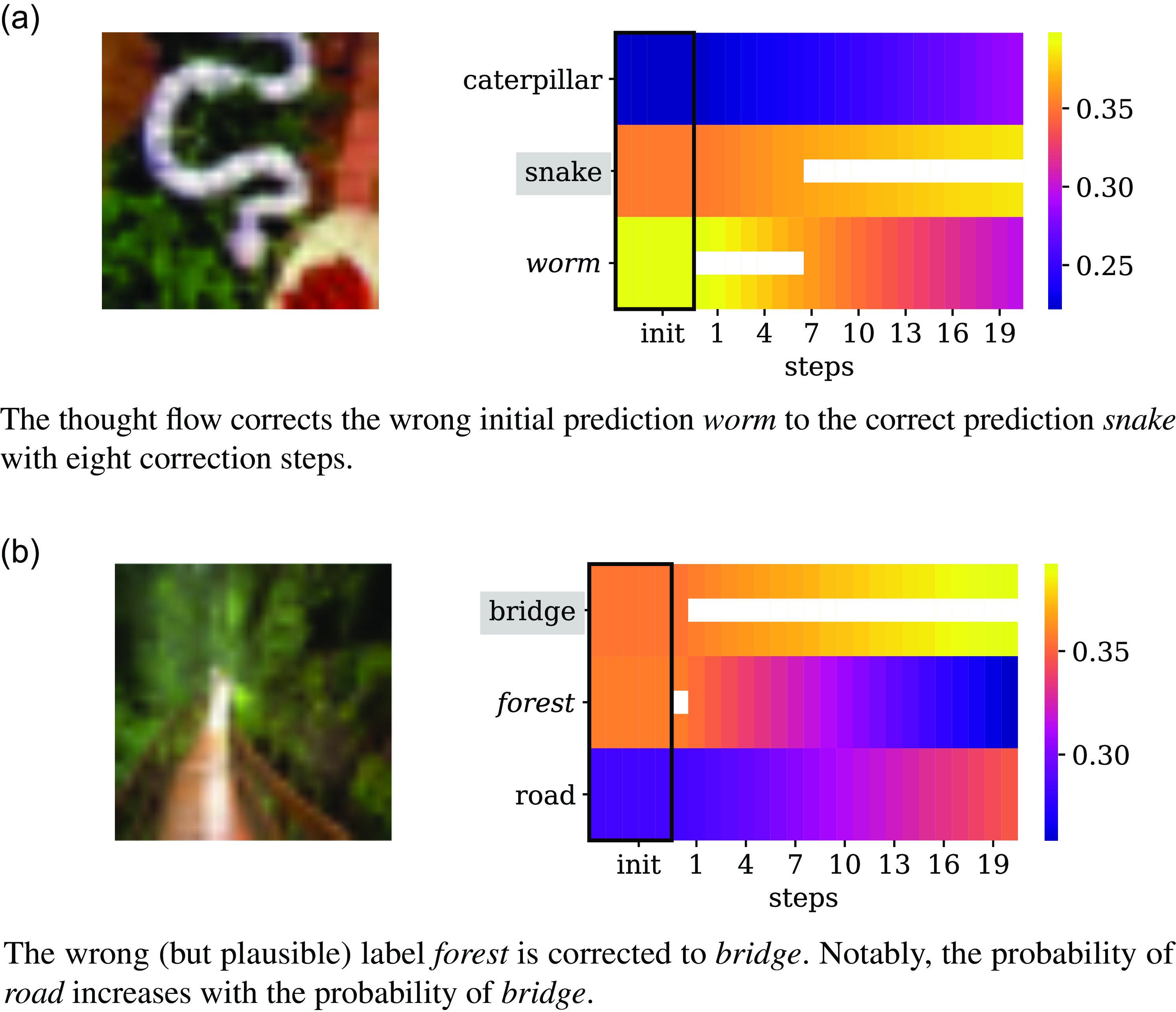
Figure 6. Exemplary thought flows on CIFAR-100 instances. The black rectangle shows the initial class probabilities from the base model (step 0), that is, the unmodified prediction, from a bird’s eye perspective. The corresponding predicted label is marked in italics. On the right side of the black rectangle, the thought flow is depicted. The white lines mark the maximum probability across classes for each step. The ground-truth label is marked with a gray box. For readability, we only show classes that reach a probability of at least 1% within the thought flow.
We provide a detailed analysis of thought flow patterns for image classification similar to our analysis for QA in Section 3.3 in Appendix D.
Overall, we observe that our thought flow method is applicable beyond QA and can correct model predictions of image classifiers. As for the QA thought flow patterns discussed in Section 3.3, we observe numerous correction patterns that exhibit a surprisingly high complexity and motivate a deeper study of the correction dynamics in future work.
6. Related work
6.1 Cognitive modeling and systems
The fields of cognitive modeling and cognitive systems have developed and evaluated numerous theories and models of human thinking (Rupert Reference Rupert2009; Busemeyer and Diederich Reference Busemeyer and Diederich2010; Levine Reference Levine2018; Lake et al. Reference Lake, Ullman, Tenenbaum and Gershman2017). While work in these fields is often oriented towards accurate descriptions of human cognition, our method does not aim to provide a plausible description of cognitive process per se. We instead aim to apply a mature, well-studied philosophical concept to machine learning in order to improve classification performance and user utility.
6.2 Confidence estimation
Of the existing methods to estimate a model’s confidence and the correctness of its predictions, the broader approach which trains secondary models for predicting the main model’s uncertainty (e.g., Blatz et al. Reference Blatz, Fitzgerald, Foster, Gandrabur, Goutte, Kulesza, Sanchis and Ueffing2004; DeVries and Taylor Reference DeVries and Taylor2018) is the closest to our work. ConfidNet (Corbière et al. Reference Corbière, Thome, Bar-Hen, Cord and Pérez2019) is particularly relevant to our approach as it predicts the true-class probability of the main model. In contrast, our correction module receives the class probabilities of the main model as input and predicts a correctness score. Unlike methods which aim at estimating accurate confidence scores, we predict such scores only as an auxiliary task in order to generate a gradient that allows us to update the model prediction.
6.3 Model corrections
Regarding model correction, the arguably most established approach to learning corrections of model predictions is gradient boosting (Friedman Reference Friedman2001) including its popular variant XGBoost (Chen and Guestrin Reference Chen and Guestrin2016). Unlike these methods which aim at using an ensemble of weak learners, we propose a lightweight correction module that is applicable on top of any existing classification model. Furthermore, in our method, the correction module receives the main model’s predictions and is able to directly adapt them.
6.4 Sequences of predictions
The idea of iteratively predicting and correcting model responses has been explored for a long time. Early work includes Mori et al. who present a non-neural iterative correction method tailored to estimate elevation maps from aerial stereo imagery (Mori, Kidode, and Asada Reference Mori, Kidode and Asada1973). Katupitiya et al. propose to iterate two neural networks to address the problem of predicting inputs of a mechanical process given the outputs of the process (Katupitiya and Gock Reference Katupitiya and Gock2005). While their method is specifically designed for the task of input prediction, our work presents a general-purpose classification model that iterates class label predictions.
Besides those task-specific methods, there are models and inference methods that make use of an iterative prediction process by design, such as Hopfield networks (Hopfield Reference Hopfield1982) and their modern variants (Barra, Beccaria, and Fachechi Reference Barra, Beccaria and Fachechi2018; Ramsauer et al. Reference Ramsauer, Schäfl, Lehner, Seidl, Widrich, Gruber, Holzleitner, Pavlovic, Sandve, Greiff, Kreil, Kopp, Klambauer, Brandstetter and Hochreiter2020), or Loopy Belief Propagation, Markov Chain Monte Carlo or Gibbs sampling (Bishop Reference Bishop2006; Koller and Friedman Reference Koller and Friedman2009). While these techniques can be linked to our work conceptually, they all require a new model to be trained. In contrast, our approach can be applied to an existing neural model as well.
6.5 Chain-of-thought, tree-of-thoughts, and self-refine
Another related line of work uses particular prompting strategies to improve the output of language models.
In chain-of-thought (CoT) prompting (Wei and Wang Reference Wei and Wang2022), the language model is prompted with examples of expected answers, correct/incorrect examples, problem decomposition, or reasoning in a few-shot or one-shot manner which are likely to bias, condition, and ground the large language model in its responses. A typical zero-shot variant of CoT prompting is, for example, to append “Let’s think step by step” to the prompt (Kojima et al. Reference Kojima, Gu, Reid, Matsuo and Iwasawa2022).
While CoT prompting methods can yield improved model responses, they (a) typically predict only one answer which provides an opaque view of the models’ deduction and reasoning steps without changing or correcting the answer itself and (b) are restricted to a textual input domain. In contrast, our method is applicable to any domain that can be transformed into a vector representation such as images, sound, or graphs. In addition, while CoT prompting yields one answer that contains information on its deduction without changing or correcting its answer (i.e., it cannot be applied iteratively), our method is not specifically targeted towards decomposition/reasoning in that it predicts a sequence of answers towards the goal of iteratively improving the answer with every iteration.
As a generalization of chain-of-thought-prompting, tree-of-thoughts prompting (Yao et al. Reference Yao, Yu, Zhao, Shafran, Griffiths, Cao and Narasimhan2023) explores sampled candidate solutions using a heuristically guided tree search. Similar to our approach, this enables iterative decision updates. However, tree-of-thought-prompting is limited to textual inputs and can only represent discrete decision changes instead of the smooth solution space exploration provided by our method. We refer to the survey of Yu et al. (Reference Yu, He, Wu, Dai and Chen2023) for an exhaustive taxonomy of CoT prompting strategies.
Similarly, Madaan et al. (Reference Madaan, Tandon, Gupta, Hallinan, Gao, Wiegreffe, Alon, Dziri, Prabhumoye, Yang, Gupta, Majumder, Hermann, Welleck, Yazdanbakhsh and Clark2023) propose Self-Refine, a prompt-based method that is used to iteratively generate an initial response, textual feedback to that response, and a subsequently updated response. While Self-Refine and our method share the paradigm of iterative self-critique and response revision, Self-Refine is constrained to the textual domain and requires the underlying model to be a text generation model that supports the method’s feedback and revision prompts, while our method can be applied to arbitrary domains and supports any type of model. This difference to our method equally applies to numerous other variants of Self-Refine such as Self-Correct (Welleck et al. Reference Welleck, Lu, West, Brahman, Shen, Khashabi and Choi2023) and Reflexion (Shinn et al. Reference Shinn, Cassano, Gopinath, Narasimhan and Yao2023).
Building upon the insights reported by Dai et al. (Reference Dai, Sun, Dong, Hao, Ma, Sui and Wei2023), who show that in-context learning can have a similar effect as explicit finetuning, we hypothesize that the described prompt-based methods can potentially be linked to our method via the approximately dual form between Transformer attention and gradient descent.
6.6 Learning to stop
In another related line of work, namely ACT (Graves Reference Graves2016) and PonderNet (Banino, Balaguer, and Blundell Reference Banino, Balaguer and Blundell2021) recurrent networks are trained to learn when to stop applying recurrent transformations within the model. While their approaches call for recurrent modules and base model retraining, our method only requires the model to yield output logits and leaves the base model unchanged.
7. Limitations and future work
The previous results demonstrate that our thought flow method can improve model performance (Section 3.2) as well as users’ system perception and human-AI performance (Section 4.2). However, its successful application to improve model performance is yet bound to limitations. The reasons for its utility for users needs to be systematically explored, and its potential to be applied to a broad range of domains and tasks should be exploited. In the following, we detail these three aspects and propose concrete directions for future work.
7.1 Stopping heuristics
This paper conducts an initial exploration of the thought flow method’s feasibility and demonstrates that the proposed training and inference algorithms can successfully be applied to a complex QA task and on top of the prevalent Transformer architecture. However, our experiments in Section 3.2 also show that a crucial factor of its successful application is to stop prediction modifications (a) late enough to enable class label changes but (b) early enough to prevent “overshooting” modifications that, despite an initial prediction improvement, deteriorate the prediction in later modifications. We hypothesize that this challenge can be successfully tackled by heuristically exploiting (i) geometric features of the thought flow (e.g., smooth transitions could potentially signal desirable prediction modifications while sharp and sudden changes could signal overshooting), (ii) decaying gains in self-estimated correctness (e.g., as soon as the model’s correctness score estimates improvements per prediction update fall below a threshold, the corresponding prediction updates might not yield additional improvements), or (iii) considering thought flows as dynamic systems and deriving stopping criteria from established characteristics. Concretely, we argue that the study of curvature can be a promising first step for geometry-related stopping heuristics, a running average over self-estimated correctness differences between iterations can be applied for correctness score-related stopping heuristics, and Lyapunov exponents (Dieci and Van Vleck Reference Dieci and Van Vleck2002) should be studied for stopping heuristics considering thought flows as dynamic systems. We expect that future work will be able to develop stopping heuristics by exploring these directions either in isolation or in combination and thereby enable real-world deployment of the thought flow method.
7.2 Underlying effects on human perception
Our results in Section 4.2 show that thought flows are better or equally good than both (a) single predictions and (b) top-3 predictions. While many of the improvements of thought flows over single predictions can also be achieved by providing users with top-3 predictions, top-3 predictions induce a cost of significantly increased completion times. These observations raise the question of how thought flows differ from top-3 predictions regarding human perception such that they enable equal or better user interaction. We expect that answering this question requires to explore how thought flow versus top-3 predictions can be related to humans’ processing of sequential versus simultaneous presentation. Concretely, we hypothesize thought flows to be associated with sequential presentation and top-3 predictions with simultaneous presentation. Related work in psychology found simultaneous presentation to be associated with a focus on the difference between options and an attention shift away from common information (Basu and Savani Reference Basu and Savani2018) and—in specific conditions—worse decisions than sequential presentation (Read et al. Reference Read, Antonides, Van den Ouden and Trienekens2001). Future work should explore this potential relation between thought flows and users’ processing of sequential presentation.
7.3 Applicability to further tasks and domains
In this paper, we introduced our thought flow method with the example of a QA task in the text domain. However, as it only requires a model to provide a vector representation of the model input and a differentiably linked model output, it can be applied to the vast majority of classification models within as well as outside natural language processing. In general, we expect that our method will yield promising results in any task for which predicting the correct answer is substantially harder than verifying whether a given answer is plausible. We thus hypothesize that our method will be particularly useful for tasks that involve (a) multiple reasoning steps, (b) structured predictions, or (c) generation. Beyond the multi-step QA task we explored, multi-step reasoning tasks in NLP include multi-step reading comprehension (Lin et al. Reference Lin, Tafjord, Clark and Gardner2019) or multi-step numerical reasoning (Zhao et al. Reference Zhao, Li, Li and Zhang2022). Structured prediction tasks in NLP include, i.a., dependency parsing or multi-label document classification. A concrete example of a generation task is dialog systems for which our flow method could prevent systems from generating inconsistent responses by re-assessing their answer generation with respect to the dialog history. In addition, our method is agnostic to the input domain, motivating various applications in the vision domain, such as scene comprehension or image segmentation.
8. Conclusion
In this paper, we introduced a task-agnostic self-correction formalism that turns a model’s single output prediction into a “thought flow”—an evolving sequence of predictions. We draw inspiration from Hegel’s dialectics and propose a correction module along with a gradient-based update rule that sequentially updates a model’s output distributions in the direction of an increasing self-estimate of correctness. We incorporate our method into existing QA models and conduct extensive experiments which include downstream human evaluation. Our experimental results indicate that thought flows (i) can increase $\text{F}_1$
-scores by up to 9.3%, (ii) exhibit complex self-modification patterns, (iii) provide significant improvements in human interaction and system perception including task performance as measured in task performance and perceived system correctness and naturalness, and (iv) can be applied to further domains, such as computer vision. A potential next step to further improve performance is a mechanism to learn when to stop the modification procedure for which we discuss different heuristic approaches.
$\text{F}_1$
-scores by up to 9.3%, (ii) exhibit complex self-modification patterns, (iii) provide significant improvements in human interaction and system perception including task performance as measured in task performance and perceived system correctness and naturalness, and (iv) can be applied to further domains, such as computer vision. A potential next step to further improve performance is a mechanism to learn when to stop the modification procedure for which we discuss different heuristic approaches.
Competing interests
The authors declare none.
Appendix A. Relation to Hegel’s dialectics
Dialectics, in general, refers to a family of methods pertaining to philosophical argumentation that involves contradictory processes between opposing sides (Maybee Reference Maybee2020). What distinguishes Hegel’s dialectic from other dialectics is that in his dialectic the opposing sides are views or definitions while the most classic version, Plato’s dialectic, treats people as the opposing sides, for example Maybee (Reference Maybee2020). While there is a variety of dialectics that can potentially inspire the development of novel machine learning methods (see, e.g., the overview of dialectics by Kuçuradi Reference Kuçuradi1990), we choose to build upon Hegel’s dialectics due to its philosophical relevance and maturity as well as its relation to various fields, such as cognitive sciences (Riegel Reference Riegel1973), neuroscience (Boonstra and Slagter Reference Boonstra and Slagter2019), or constraint satisfaction and optimization (Kadioglu and Sellmann Reference Kadioglu and Sellmann2009).
A.1 Relation to thesis-antithesis-synthesis triads
The three moments are often compared to the thesis-antithesis-synthesis pattern in philosophy popularized by Heinrich Moritz Chalybäus, but are not necessarily equal (Mueller Reference Mueller1958). A more detailed discussion of the thesis-antithesis-synthesis triad and its difference to the three moments is provided by Maybee (Reference Maybee2020). While the thesis-antithesis-synthesis triad suggests a singular dialectical “one-pass” process of thinking and reasoning, Hegel’s dialectical process allows for several iterations and does not have to end after a single iteration (Maybee Reference Maybee2020). A particular example of such an iterative process within Hegel’s work can be found in the dialectical development of Hegel’s logic regarding the concepts of “Abstract Purpose” and “Realized Purpose” (Maybee Reference Maybee2020). The fundamental “multi-pass” notion of multiple iterations of thinking and reasoning forms the basis for of our thought flow approach.
Appendix B. Question answering experiments
B.1 Data set details
We use the HotpotQA data set (Yang et al. Reference Yang, Qi, Zhang, Bengio, Cohen, Salakhutdinov and Manning2018), which is an English multi-hop QA data set. It covers 90,564 training instances, 7,405 test validation instances, and 7,405 test instances per setting (there are a distractor and a fullwiki setting). Training instances are grouped by difficulty and cover 18,089 easy, 56,814 medium, and 15,661 hard questions. We refer to Yang et al. (Reference Yang, Qi, Zhang, Bengio, Cohen, Salakhutdinov and Manning2018) for more details.
B.2 Additional modification examples
Table B1 displays additional examples for each of the emerging thought flow patterns discussed in Section 3.3.
B.3 Changes in precision and recall
Figure B1 shows the fractions of instances with an observed increase or decrease in precision and recall across different $\delta$
values.
$\delta$
values.
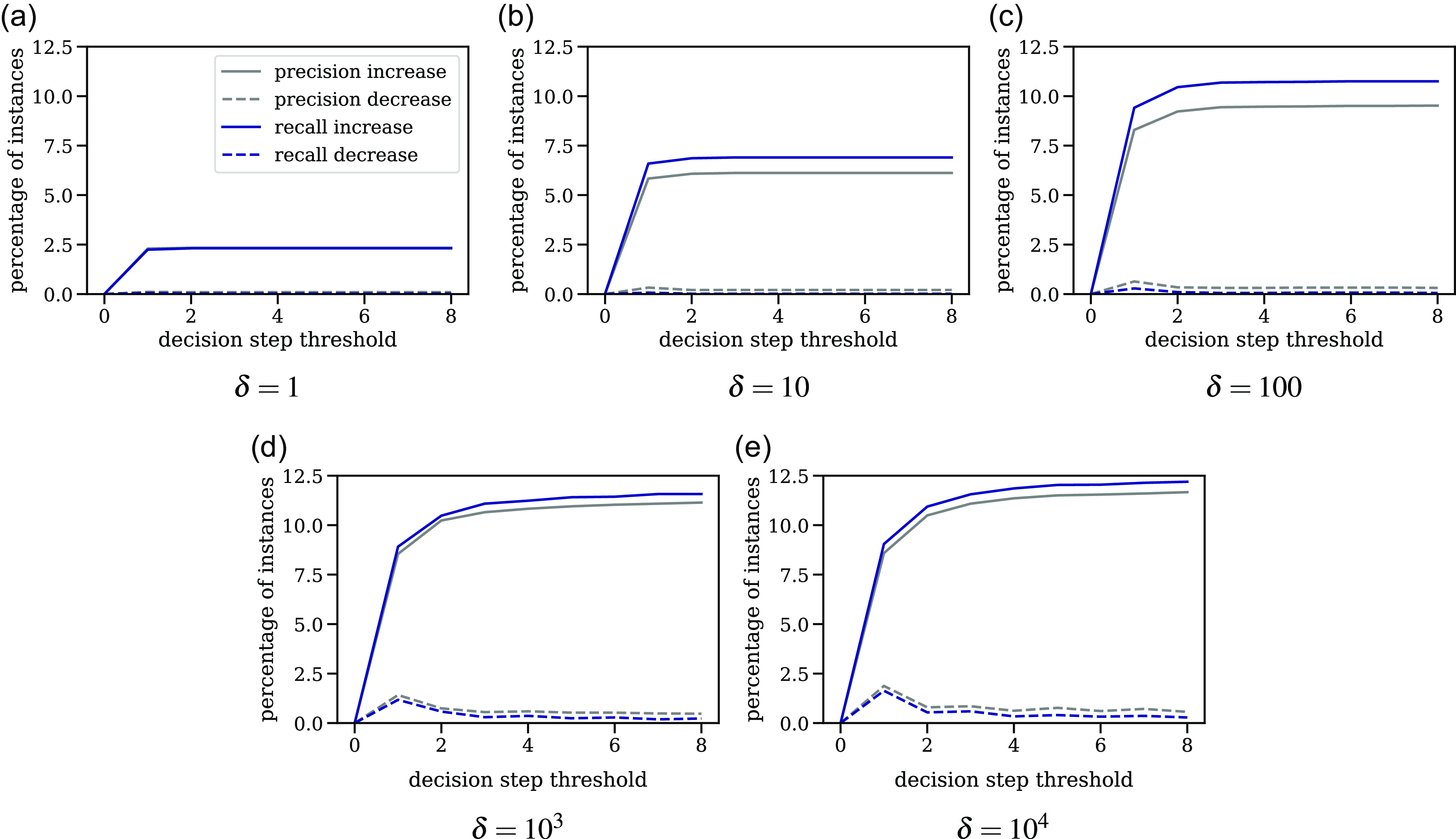
Figure B1. Fraction of instances for which a thought flow with different decision step thresholds results in increased or decreased values of precision and recall.
Table B1. Additional examples of the modification patterns presented in Table 2. The correct answer is marked in bold, and the predicted answer per flow step is marked in orange
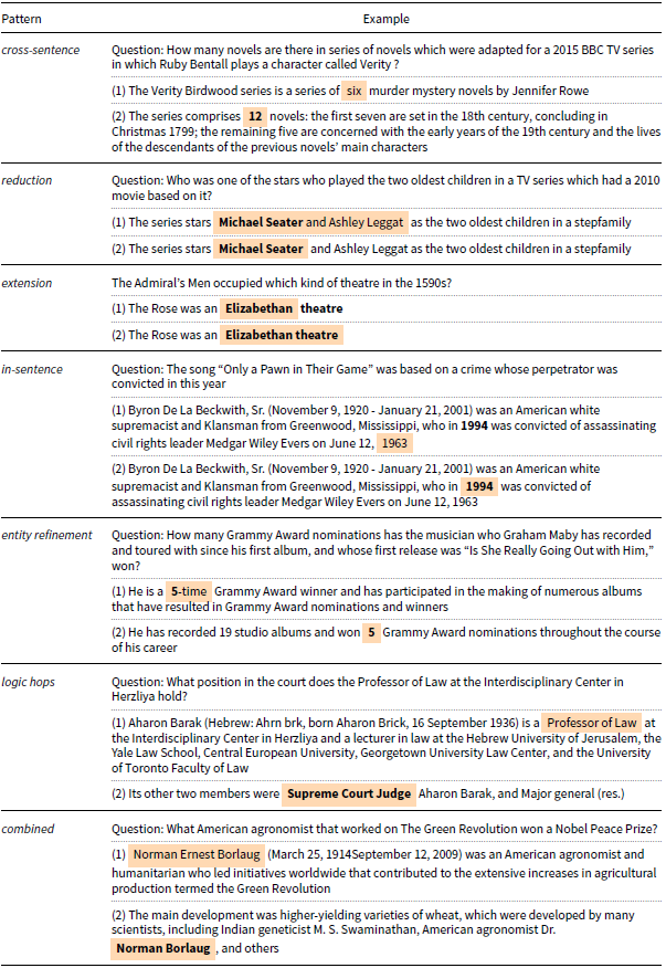
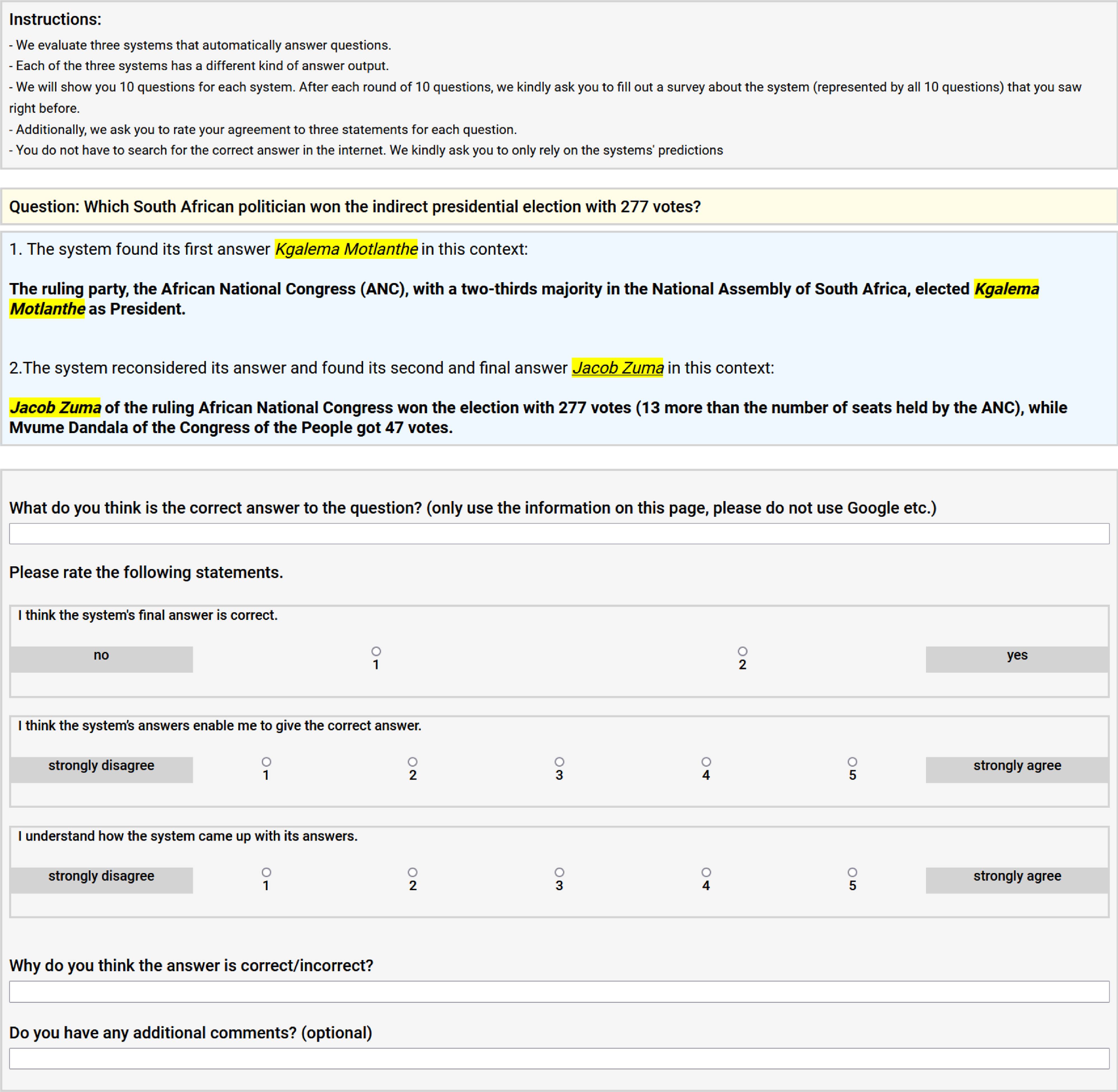
Figure C1. User study interface showing the TF condition (ours).
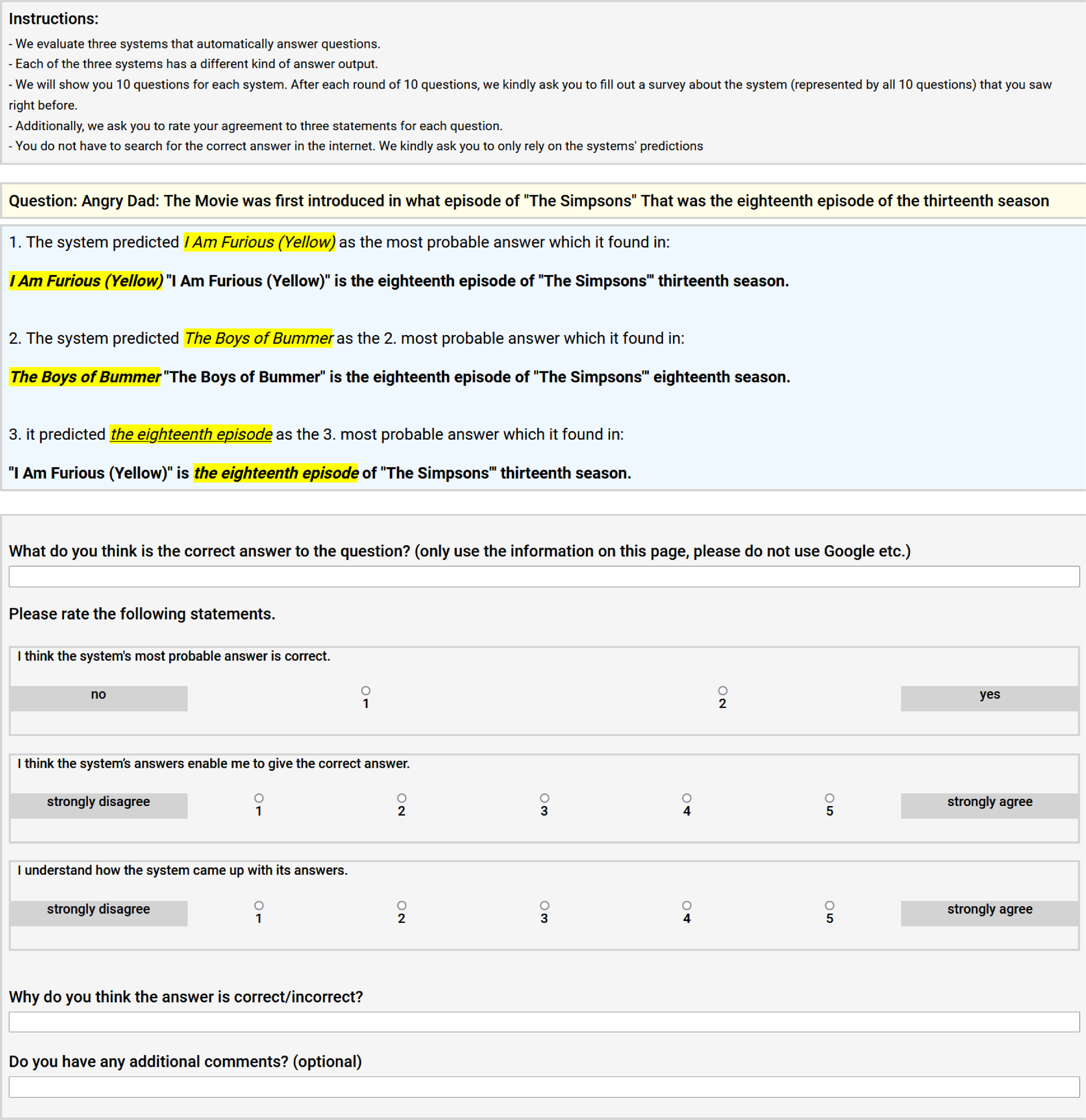
Figure C2. User study interface showing the top-3 condition.
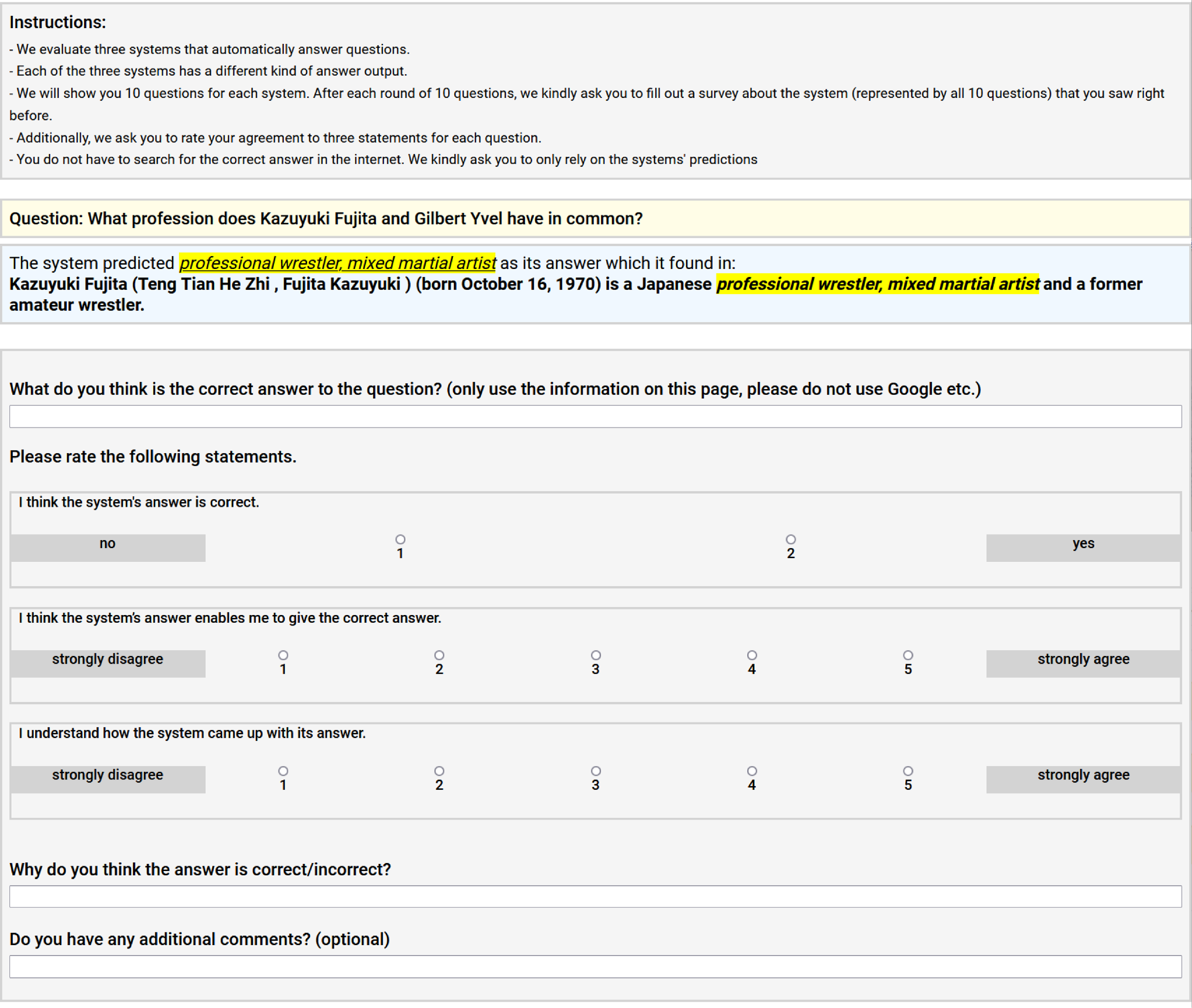
Figure C3. User study interface showing the single condition.
Appendix C. User study
C.1 Questionnaire items
C.1.1 Per-system questionnaires
Usability. The UMUX usability scale (Finstad Reference Finstad2010, Reference Finstad2013) uses the following four 5-point Likert items:
-
• This system’s capabilities meet my requirements.
-
• Using this system is a frustrating experience.
-
• This system is easy to use.
-
• I have to spend too much time correcting things with this system.
Mental Effort. The Pass mental effort scale usability scale (Paas Reference Paas1992) uses a single 9-point Likert item:
-
• Please rate the mental effort required to decide if the system’s answer is correct. (The 9 points are labeled from “very, very low mental effort” to “very, very high mental effort.”)
Anthropomorphism. The Godspeed anthropomorphism subscale (Bartneck et al. Reference Bartneck, Kulic, Croft and Zoghbi2009) uses five 5-point semantic differential scales that ask the user to rate the system in a spectrum of:
-
• fake – natural
-
• machine-like – human-like
-
• unconscious – conscious
-
• artificial – lifelike
-
• (moving rigidly – moving elegantly) (We exclude this item as it is not applicable to QA systems.)
Perceived Intelligence. The Godspeed perceived Intelligence subscale (Bartneck et al. Reference Bartneck, Kulic, Croft and Zoghbi2009) uses five 5-point semantic differential scales that ask the user to rate the system in a spectrum of:
-
• incompetent – competent
-
• ignorant – knowledgeable
-
• irresponsible – responsible
-
• unintelligent – intelligent
-
• foolish – sensible
C.1.2 Per-item questionnaires
Perceived Answer Correctness. We use a single binary item to collect perceived answer correctness ratings:
-
• I think the system’s answer is correct.
Perceived Helpfulness. We use a single 5-point Likert item to collect helpfulness ratings:
-
• I think the system’s answer enables me to give the correct answer.
Perceived Understanding. We use a single 5-point Likert item to collect understanding ratings:
-
• I understand how the system came up with its answer.
C.2 Interface
Figures C1, C2, C3 show screenshots of our experiment interface for the three studied prediction conditions TF, top-3 and single. Figure C4 depicts an attention check question.
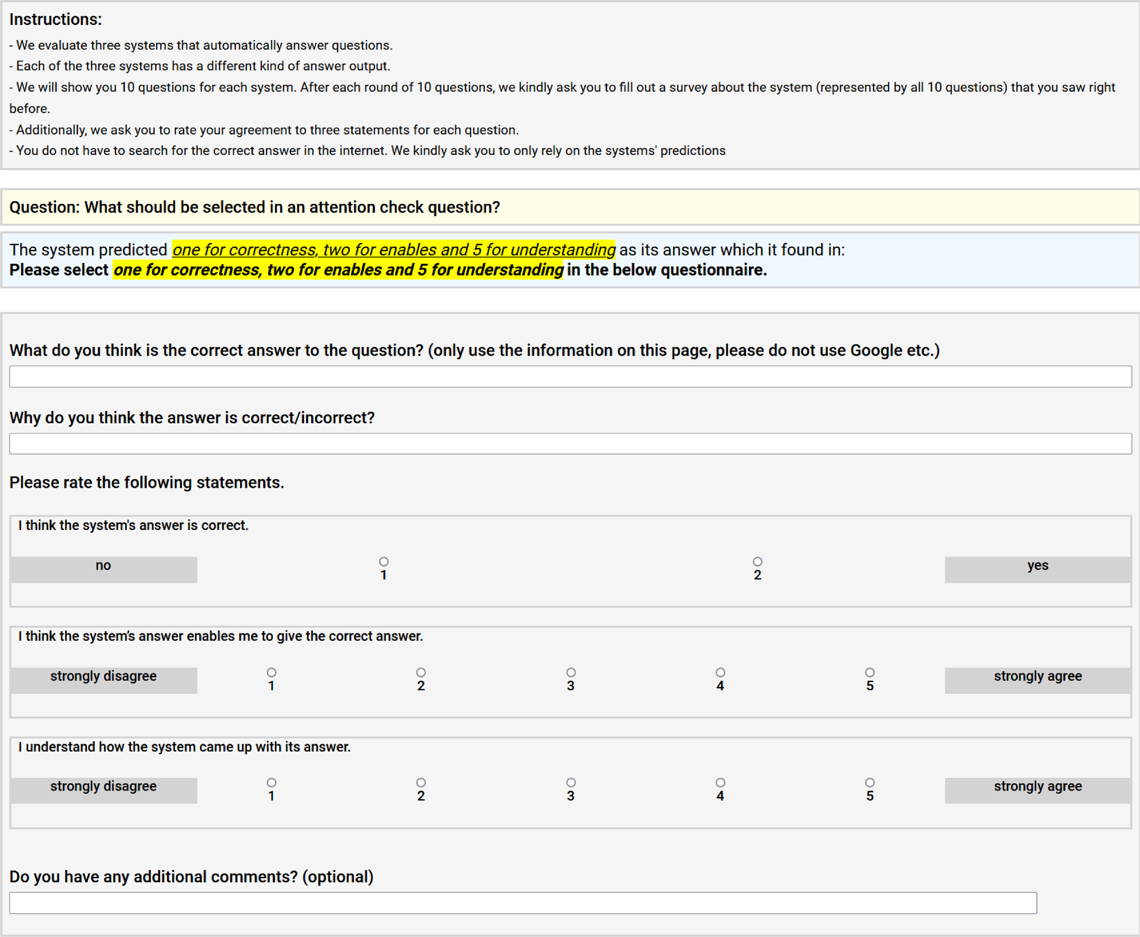
Figure C4. User study interface showing an attention check.
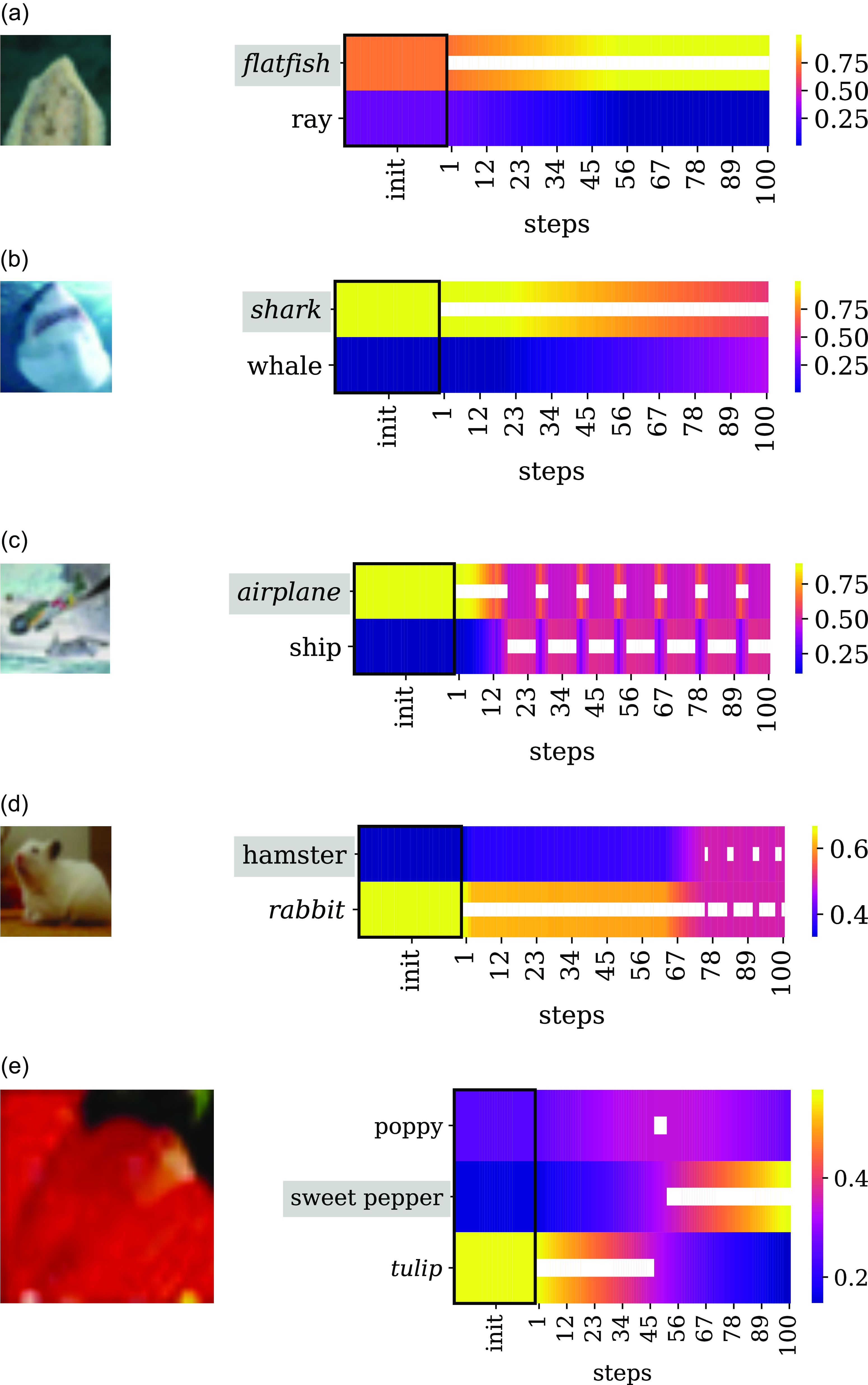
Figure D1. Exemplary thought flows from different models on CIFAR demonstrating the diverse range of correction dynamics. A detailed description of the plots is provided in Fig. 6.
Appendix D. Image classification thought flow patterns
Similar to the qualitative analysis of flow patterns in our QA experiments (see Section 3.3), we now investigate the dynamics of the generated image classification thought flows. While Fig. 6 shows thought flows that gradually transition from one class to another and then converge to that class, we observe diverse flow patterns which we display in Figs. D1 and D2. Fig. D1(a) shows an example for which our method does not change the (correct) label prediction but increases the model’s confidence in its prediction. In Fig. D1(b), the thought flow does not change the predicted label but decreases the model’s confidence. Thus, the flows in Fig. D1(a),(b) can be interpreted as a form of neural network calibration (Reference Guo, Pleiss, Sun and WeinbergerGuo et al. 2017). Fig. D1(d) shows a smooth transition from one class to a gradual back-and-forth between two classes. In Fig. D1(e) one can see a transition from the class tulip to the class sweet pepper via the class poppy. In Fig. D2(a), the thought flow quickly changes from plain to cloud. While the predicted class remains cloud, the probability of plain decreases continuously until the flow changes its prediction to sea which we interpret as overthinking (Kaya, Hong, and Dumitras Reference Kaya, Hong and Dumitras2019). Fig. D1(b),(c),(c),(d) show different periodic behaviors including the transition from a cycle to a fixed class in Fig. D2(b), smooth cycles in Fig. D1(c) and longer sawtooth-like cycles in Fig. D2(d). Importantly, Fig. D2(b), (e) are examples for flows that explore an alternative class prediction but “return” to the initial class prediction and thus show that our method can be used to explore alternatives without necessarily neglecting a correct prediction.
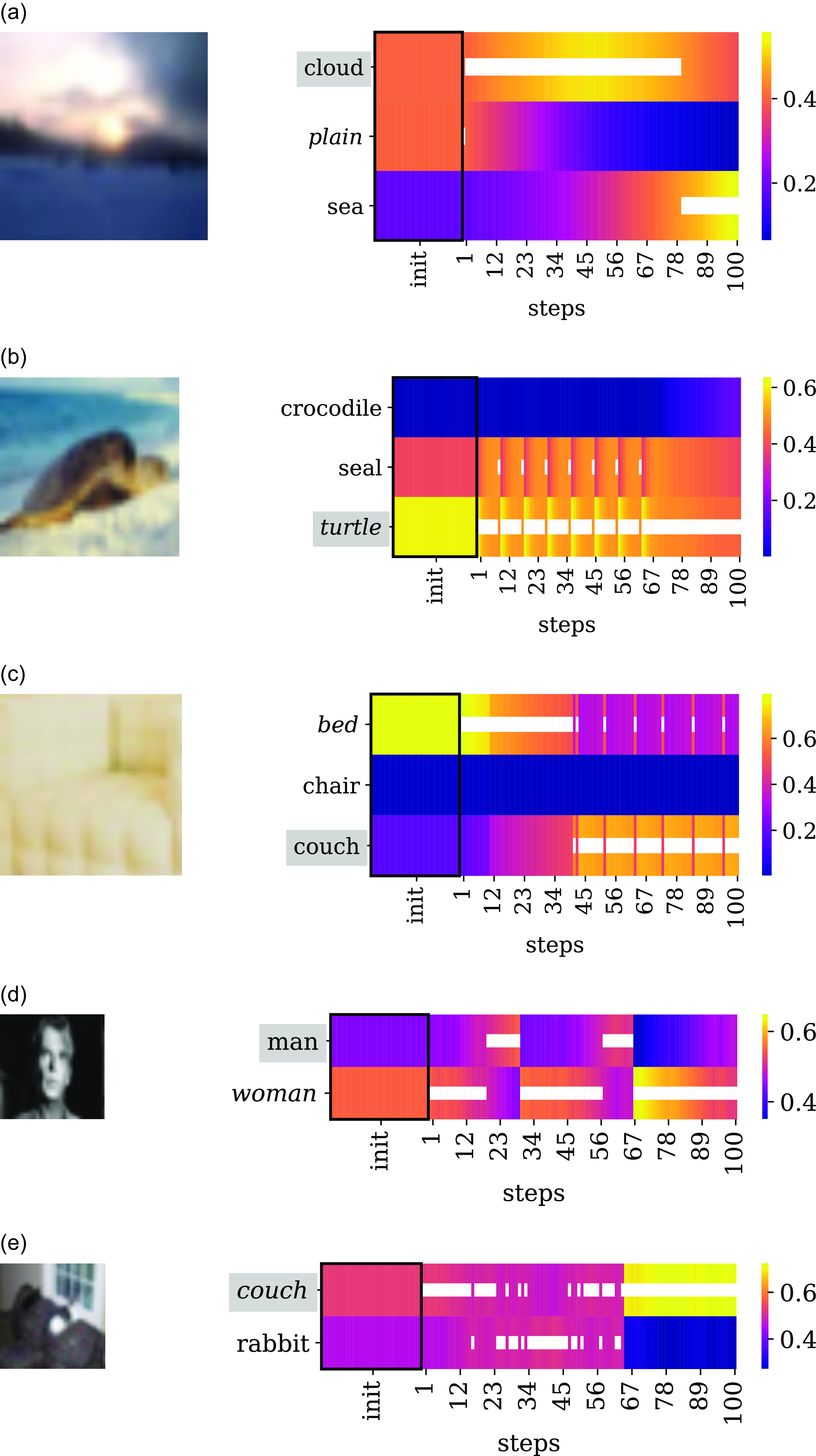
Figure D2. More exemplary thought flows from different models on CIFAR demonstrating the diverse range of correction dynamics. A detailed description of the plots is provided in Fig. 6.


 Open access