


Introduction
The response of the coastal zone to global sea-level rise is highly variable. Knowledge of parameters controlling coastal change alongside the regional sea-level history is therefore indispensable when the response to global sea-level rise is to be assessed. The relative sea level (RSL) at any given coastal site depends on different factors such as climatically induced global changes, regional vertical movements of the lithosphere including tectonics and glacial isostatic adjustment (GIA). In addition, local factors influence RSL. These are most notably compaction and coastal geomorphology influencing tides, local water levels and sedimentary processes (e.g. Baeteman, Reference Baeteman1999; Kiden et al., Reference Kiden, Denys and Johnston2002; Long et al., Reference Long, Waller and Stupples2006; Steffen, Reference Steffen2006; Vink et al., Reference Vink, Steffen, Reinhardt and Kaufmann2007; Kiden et al., Reference Kiden, Makaske and van de Plassche2008; Bungenstock & Weerts, Reference Bungenstock and Weerts2012; Karle et al., Reference Karle, Bungenstock and Wehrmann2021). These factors act on different time and spatial scales and result in geomorphological changes like progradation and retrogradation of the coastline. Natural hazards such as storm surges may cause severe and abrupt changes to the coastal geomorphology and may trigger long-lasting inundation.
This study presents a reconstruction of RSL for the area of the East Frisian island Langeoog, representative for the East Frisian barrier island coast. A precursor curve was published in Bungenstock & Schäfer (Reference Bungenstock and Schäfer2009). The data points of that curve were derived from intercalated peat data. This was based on the idea that sea-level fluctuations could only be proved by intercalated peat data. However, based on the plotted age data, no sea-level fluctuations in the sense of sea-level drops could be shown. Nevertheless, relying on the idea that intercalated peats clearly indicate a change of RSL, the data points were connected in a step-like manner to hypothesise still-stand phases of RSL instead of sea-level drops as proposed by Behre (Reference Behre2003, Reference Behre2007). In the following years, there was continuing discussion on the robustness of derived sea-level fluctuations and the resolution of field data to prove these (Bungenstock & Weerts, Reference Bungenstock and Weerts2010, Reference Bungenstock and Weerts2012; Baeteman, Reference Baeteman, Waller and Kiden2011, 2012; Behre, Reference Behre2012a,b). The standardised ‘protocol for a geological sea-level database’ (Hijma et al., Reference Hijma, Engelhart, Törnqvist, Horton, Hu, Hill, Shennan, Long and Horton2015) and the standardised global synthesis of regional RSL data (Khan et al., Reference Khan, Horton, Engelhart, Rovere, Vacchi, Ashe, Törnqvist, Dutton, Hijma and Shennan2019) now allow for a reinterpretation of the data of Bungenstock & Schäfer (Reference Bungenstock and Schäfer2009). Therefore, we present a review and reinterpretation of the sea-level data for the area of Langeoog including all available archive data and newly collected data.
Short review of ideas, opinions and approaches regarding Holocene sea-level research along the German North Sea coast
Research and concepts on Holocene relative sea-level rise along the German North Sea coast have an almost 100-year-long history. The first Holocene RSL curve was published by Schütte (Reference Schütte1939). He suggested a sinking coast and no eustasy-related sea-level rise. Relating to the peat layers intercalated in the Holocene sedimentary record along the southern North Sea coast, Schütte assumed an isostatic sinking of the coast interrupted by three rising phases. Nilsson (Reference Nilsson1949) followed this idea, including the geographical differences of the mean tidal high-water level, to relate data from different areas along the German North Sea coast to each other (see also Louwe Kooijmans, Reference Louwe Kooijmans1976).
Haarnagel (Reference Haarnagel1950) suggested that beside isostasy, eustasy is a relevant factor for RSL along the German North Sea coast. He used basal peat data to exclude errors caused by compaction, and included settlement dynamics to differentiate better amongst transgression and regression phases during the late Holocene (Haarnagel, Reference Haarnagel1950).
In a seminal paper, Jelgersma (Reference Jelgersma, Ole, Schüttenhelm and Wiggers1979) published the RSL curve for the southern North Sea region. She suggested that the controlling factors are eustasy, isostasy and tectonics, with isostasy and tectonics maybe neglibible in the southern North Sea. Her RSL curve is based on radiocarbon data of the base of basal fen peats to avoid errors caused by compaction. The onset of basal fen peat growth can be initiated by local topography and drainage water from the hinterland, which means that fen peat growth is not always in direct correlation with sea level. However, it is not possible to document sea-level fluctuations when data points are exclusively derived from basal peat data (Jelgersma, Reference Jelgersma, Ole, Schüttenhelm and Wiggers1979). In fact, Louwe Kooijmans & Knip (Reference Louwe-Kooijmans and Knip1974) and Roeleveld (Reference Roeleveld1974) interpreted the intercalated peats as indicators for possible sea-level drops.
Kiden et al., (Reference Kiden, Denys and Johnston2002) compared the sea-level curves of Jelgersma (Reference Jelgersma, Ole, Schüttenhelm and Wiggers1979), Van de Plassche & Roep (Reference Van de Plassche, Roep, Scott, Pirazzoli and Honig1989), Roep & Beets (Reference Roep and Beets1988) and Denys & Baeteman (Reference Denys and Baeteman1995) and discussed the influence of spatially variable glacio-hydro-isostatic subsidence along the Belgian and Netherlands coast. They concluded that the local variability is too large to establish a general RSL curve for the southern North Sea region, but that every area of c.50 km diameter has its own RSL curve (Kiden et al., Reference Kiden, Denys and Johnston2002). Behre (Reference Behre2003, Reference Behre2007) published a RSL curve for the entire German North Sea coast. For the last 2000 years he used archaeological data by referring these to mean high water. The problem of different mean high-water levels is solved by referring and correcting all data to the Wilhelmshaven tide gauge (Behre, Reference Behre2003, Reference Behre2007). Similar to Jelgersma (Reference Jelgersma, Ole, Schüttenhelm and Wiggers1979), Behre regards the glacial isostatic adjustment along the southern North Sea coast as insignificant. His curve is characterised by several wiggles marking sea-level fluctuations of up to 2 m within 200 years.
Ervynck et al., (Reference Ervynck, Baeteman, Demiddele, Hollevoet, Pieters, Schelvis, Tys, Van Strydonck and Verhaeghe1999) and Baeteman (Reference Baeteman1999) related the shifting coastline during the middle and late Holocene to different rates of aggradation when sediment supply outpaces the creation of accommodation space, which could differ from place to place. Baeteman (Reference Baeteman1999) showed that, for example, a facies shift from mud flat to peat depends on the relative proximity to tidal channels, their migration and sediment supply. Therefore, the intercalated peats are regarded as local phenomena with little significance for RSL reconstruction. With four transects along the East Frisian Peninsula, Streif (Reference Streif2004) showed that the intercalated peat beds have different ages in the different areas apart from the uppermost peat layer situated at −1 to 0 m NN (German Ordnance Datum) which is dated to c.2000 BP in all transects.
In addition, intercalated peat beds are always affected by compaction (e.g. Streif Reference Streif1971; Baeteman, Reference Baeteman1999; Bungenstock & Schäfer, Reference Bungenstock and Schäfer2009; Horton & Shennan, Reference Horton and Shennan2009; Engelhart & Horton, Reference Engelhart and Horton2012) and have to be carefully evaluated before being used for sea-level reconstructions. On the other hand, possible Holocene RSL fluctuations can only be documented by including sea-level index points (SLIPs) from intercalated peat layers sandwiched in the Holocene geological record or by data derived from, for example, foraminifera transfer functions. Plotting data exclusively from basal peat beds could only show possible slowdowns of RSL, but not a sea-level fall (Jelgersma, Reference Jelgersma, Ole, Schüttenhelm and Wiggers1979; Shennan et al., Reference Shennan, Hamilton, Hillier and Woodroffe2005; Brain, Reference Brain, Shennan, Long and Horton2015). Therefore, in an earlier study (Bungenstock & Schäfer, Reference Bungenstock and Schäfer2009), data derived from intercalated peat were scrutinised for compaction by interpreting the geological record in cross sections. Additionally, intercalated peat beds were evaluated for their local occurrence versus their stratigraphic meaning by correlating them over several hundreds of metres in cross sections and seismic tracks. This resulted in a RSL curve characterised by phases of slowdown or still-stand. This was in contrast to the strongly fluctuating curve of Behre (Reference Behre2007) and triggered a discussion on the interpretation of sea-level index data in terms of sea-level fluctuations for the German coast (Bungenstock & Weerts, Reference Bungenstock and Weerts2010, Reference Bungenstock and Weerts2012; Baeteman, Reference Baeteman, Waller and Kiden2011; Baeteman et al., Reference Baeteman, Waller and Kiden2012; Behre, Reference Behre2012a,b). Today, most recent sea-level reconstructions for the southern North Sea are based on base of basal peat data or ideally on dated transgressive contacts on top of a thin basal peat layer (Meijles et al., Reference Meijles, Kiden, Streurman, Van der Plicht, Vos, Gehrels and Kopp2018; Hijma & Cohen, Reference Hijma and Cohen2019). However, the most precise sea-level records, which can be derived from salt-marsh sediments for e.g. the coast of North America (Kemp et al., Reference Kemp, Horton, Vane, Bernhardt, Corbett, Engelhart, Anisfeld, Parnell and Cahill2013), Tasmania (Gehrels et al., Reference Gehrels, Callard, Moss, Marshall, Blaauw, Hunter, Milton and Garnett2012) or the British Isles (Barlow et al., Reference Barlow, Shennan, Long, Gehrels, Saher, Woodroffe and Hillier2013) and micro-atolls, show maximum oscillations in the order of 0.2 m per century (Gehrels & Shennan, Reference Gehrels and Shennan2015).
Glacial istostatic adjustment (GIA)
Kiden et al. (Reference Kiden, Denys and Johnston2002) describe a northwest- to east-southeast-orientated glacial forebulge underneath the coast of the eastern Netherlands and the western German North Sea coast referring to the geophysical isostatic models of Fjeldskaar (Reference Fjeldskaar1994), Lambeck (Reference Lambeck1995) and Lambeck et al. (Reference Lambeck, Smither and Johnston1998). The collapse of this glacial forebulge triggers different glacial isostatic adjustment rates along the southern North Sea coast. Kiden et al. (Reference Kiden, Denys and Johnston2002) therefore suggest restricting the collection of sea-level data for a RSL curve to coastal areas smaller than 50 km in diameter. Taking up the approach by Kiden et al. (Reference Kiden, Denys and Johnston2002), Vink et al. (Reference Vink, Steffen, Reinhardt and Kaufmann2007) compared the RSL curves – all related to mean sea level (MSL) – from Belgium (Denys & Baeteman, Reference Denys and Baeteman1995), the Netherlands (Jelgersma, Reference Jelgersma1961; Van de Plassche, Reference Van de Plassche1982; Kiden, Reference Kiden1995; Makaske et al., Reference Makaske, Van Smeerdijk, Peeters, Mulder and Spek2003; Van de Plassche et al., Reference Van de Plassche, Bohncke, Makaske and Van der Plicht2005) and the German North Sea coast (Behre, Reference Behre2003, Reference Behre2007). They showed that the MSL error band of northwest Germany lies significantly below those of the Netherlands and even more of Belgium, diverging progressively back in time (Vink et al., Reference Vink, Steffen, Reinhardt and Kaufmann2007). The authors therefore concluded that the German North Sea coast has been subject to considerable isostatic subsidence during the Holocene.
Moreover, the glacio-hydro-isostatic model of Steffen (Reference Steffen2006) as presented by Busschers et al. (Reference Busschers, Kasse, van Balen, Vandenberghe, Cohen, Weerts, Wallinga, Johns, Cleveringa and Bunnik2007, their fig. 10B) shows that the German North Sea coast is situated on the flank of the glacial forebulge and affected by different total uplift depending on the location along the coast. The total uplift differs by more than 20 m from the western part of East Frisia to North Frisia/Germany since 21 ka (Fig. 1).
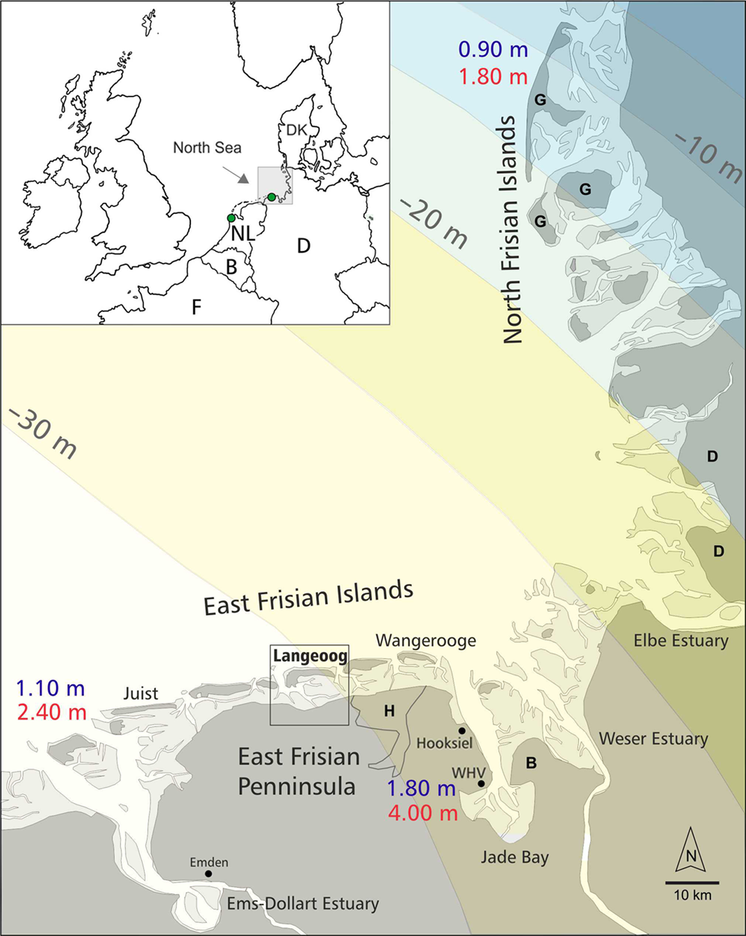
Fig. 1. The German North Sea coast. The modelled glacial isostatic adjustment (GIA) since 21 ka is pictured in shaded zones (according to Steffen, Reference Steffen2006 as presented by Busschers et al., Reference Busschers, Kasse, van Balen, Vandenberghe, Cohen, Weerts, Wallinga, Johns, Cleveringa and Bunnik2007). The different tidal range values along the coast are depicted in red, the mean high-water values in blue. The green dots in the overview frame mark the western Netherlands and study area of Hijma & Cohen (Reference Hijma and Cohen2019) and the East Frisian barrier island coast with the study area of this contribution (see Fig. 8).
G = islands with an outcropping Pleistocene core (Geestinseln); D = Dithmarschen; B = Butjadingen; H = Harle Bay around AD 1400; WHV = Wilhelmshaven.
Tides
Palaeotidal models of changing tidal range during the Holocene RSL rise in the southern North Sea show an increase in tidal range because of changing bathymetry during inundation of the shelf (Shennan et al., Reference Shennan, Lambeck, Flather, Horton, McArthur, Innes, Lloyd, Rutherford and Wingfield2000; Van der Molen & de Swart, Reference Van der Molen and de Swart2001). While the major changes occurred prior to 6 ka, only minor (cm-scale) to no changes occurred during the subsequent millennia (Shennan et al., Reference Shennan, Lambeck, Flather, Horton, McArthur, Innes, Lloyd, Rutherford and Wingfield2000; van der Molen & de Swart, Reference Van der Molen and de Swart2001). These observations are applied for the open Dutch coast, but there have not been robust observations so far to test, whether the models are valid for the back-barrier areas as well or whether the tidal amplitude may has changed on a larger scale in the tidal basins.
Another aspect to be mentioned is the spatial change of tidal range along the North Sea coast. Today, tidal range varies from lower mesotidal conditions in the west of the German North Sea coast (2.4 m at Borkum, the westernmost island of the East Frisian Peninsula) to upper mesotidal conditions in the centre (Jade Bay with 3.9 m) to lower mesotidal, almost microtidal, conditions in the North (Sylt 1.6 m) (BSH, 2020). Mean high-water level (MHW), being a function of the tidal range, differs by up to 1 m (0.9 m at Sylt and 1.9 m in the Jade Bay) (Fig. 1). Thus, spatially variable tidal ranges have to be assumed for the last millennials depending on the location of the amphidromic points, the bathymetry and the coastal profile. Consequently, the collection of RSL data needs to be restricted to small coastal areas with similar tidal conditions (Bungenstock & Weerts, Reference Bungenstock and Weerts2012).
Palaeogeography
Some examples from the German North Sea coast show that changes from semi-closed to open coasts and from a retrograding to a prograding coast and vice versa are not synchronous along the coastline. Instead, these changes strongly depend on local basin configurations and available sediment volumes as also known from the coast in the Netherlands (Beets & van der Spek, Reference Beets and van der Spek2000; Kiden et al., Reference Kiden, Makaske and van de Plassche2008).
For North Frisia for 7 ka, a peat bed is documented covering a wide coastal area (e.g. Meier et al., Reference Meier, Kühn and Borger2013). In the northern part of North Frisia, as a result of RSL rise since ∼5 ka, Pleistocene plateaus were isolated as so-called Geest islands. In the southern part of North Frisia (Dithmarschen) the coast was not protected by Pleistocene plateaus. Since 2 ka the northern part of North Frisia is characterised by continuous erosion during ongoing Holocene RSL rise, while for the southern part a positive sediment budget and, consequently, a prograding coastline is documented (Meier et al., Reference Meier, Kühn and Borger2013).
For the East Frisian coastline, Flemming & Davis (Reference Flemming and Davis1994) describe a back-barrier coast existing since 7.5 ka with spit bars accumulating at the Pleistocene ridges of the former landscape, building a closing coast. The system probably changed from micro- to mesotidal conditions around 6 ka (Shennan et al., Reference Shennan, Lambeck, Flather, Horton, McArthur, Innes, Lloyd, Rutherford and Wingfield2000; Van der Molen & Swart, Reference Van der Molen and de Swart2001; Bungenstock, Reference Bungenstock2005), with an almost closed barrier chain changing to a typical open mesotidal barrier island system and contemporaneously shifting southeastwards during Holocene RSL rise.
On the mainland, Butjadingen (Fig. 1), the land spit between Jade and Weser, prograded ∼6 km seaward during the first centuries after AD (Schmid, Reference Schmid1993; Behre, Reference Behre2012c). Some centuries later, the Harle Bay of ∼160 km2 (Fig. 1) developed at the eastern part of the East Frisian Peninsula (Behre, Reference Behre1999), later successively reclaimed by embankment.
All these findings underline the importance of collecting sea-level data from relatively small coastal sections, ideally from single tidal basins, to minimise the sources of uncertainties caused by different GIA, tidal conditions and palaeogeographic preconditions on sedimentological processes (Bungenstock & Weerts, Reference Bungenstock and Weerts2010, Reference Bungenstock and Weerts2012; Baetman et al., Reference Baeteman, Waller and Kiden2011). Comparing RSL curves from adjacent tidal basins will help to better understand and even quantify the effects in the respective areas. Therefore, Bungenstock & Weerts (Reference Bungenstock and Weerts2010) suggest collecting data for RSL curves for the German North Sea Coast representative for five different coastal sections for a first approximation. From west to east, these are (1) the Ems estuary, (2) the East Frisian Barrier island coast (including the barrier island Langeoog), (3a and 3b) the Jade Bay and the Weser estuary, (4) the Elbe estuary and (5) the North Frisian island coast (Fig. 1).
Geographical and geological setting
The German North Sea coast is situated in the southwest of the ‘Forchhammersche Linie’ (Streif, Reference Streif1990), which crosses Denmark in the NW–SE direction and which is the hinge line of the glacio-isostatic rebound caused by the postglacial melting of the Scandinavian ice cap. According to the GIA models of Kiden et al., (Reference Kiden, Denys and Johnston2002), Peltier (Reference Peltier2004), Steffen (Reference Steffen2006) as presented by Busschers et al. (Reference Busschers, Kasse, van Balen, Vandenberghe, Cohen, Weerts, Wallinga, Johns, Cleveringa and Bunnik2007), and Vink et al. (Reference Vink, Steffen, Reinhardt and Kaufmann2007), the German North Sea is situated on the flank of the collapsing glacial forebulge (Fig. 1).
The German North Sea coast is characterised by tidal flats in a mainly mesotidal regime. The depositional systems are the East Frisian barrier islands, the estuaries of the Ems, Weser and Elbe rivers, the Jade Bay with its narrow connection to the open North Sea, the North Frisian marshland islands and the North Frisian islands with their Tertiary and Pleistocene basements (Fig. 1) and the respective (mostly) back-barrier tidal flats.
In the Ems–Weser–Elbe region, for the East Frisian Peninsula with its barrier coast, the sedimentary record is characterised by Pleistocene glacial deposits disconformably overlain by Holocene sediments up to 25 m thick. The depth of the Holocene base decreases southwards. On the mainland, up to 20 km to the south of the recent coastline, Pleistocene sediments crop out at the surface. The Holocene sedimentary succession starts with a basal peat overlain by sandy, silty and clayey brackish/lagoonal and marine deposits with three to seven intercalated peat beds (Streif, Reference Streif2004). This documents distinct differences of sedimentation and sedentation processes over relatively short distances along the coast due to non-synchronous coastline shifting, erosion and redeposition (Karle et al., Reference Karle, Bungenstock and Wehrmann2021).
The back-barrier zone of Langeoog island
Langeoog is a barrier island situated in a mesotidal system (tidal range of 2.8 m; BSH, 2020). The Holocene sedimentary record in the back-barrier area of Langeoog and its adjacent mainland shows a basal peat, up to several metres thick in places close to the Pleistocene, which crops out directly south of the dike line, and up to four intercalated peat horizons, three of these occurring basin-wide and bearing stratigraphic meaning for the Langeoog area (Bungenstock & Schäfer, Reference Bungenstock and Schäfer2009).
The Holocene base ranges from −12 m NN to −4 m NN underneath the tidal flats. In the tidal inlets Accumer Ee, west of Langeoog, and the Otzumer Balje, east of Langeoog, and underneath the western part of Langeoog itself, it lies at −22 m NN in palaeo- or active channel structures (NIBIS® Map Server, 2014b).
The dike line separates the tidal flat landscape from the mainland. Since ∼700 BP (13th century AD) it was built towards the sea and made the coastline static and unable to react to RSL or single events, whereas Langeoog continuously prograded landward as a consequence of ongoing RSL rise. Maps by Homeier (Reference Homeier1964) show a migration of the island of more than 700 m since AD 1650. Over time, the combination of natural and anthropogenic processes enhanced the reworking of the tidal flat sediments (Van der Spek, Reference Van der Spek1996) and triggered the so-called Wadden Sea squeeze (Flemming & Nyandwi, Reference Flemming and Nyandwi1994), which describes the diminishing tidal flats and especially the loss of mudflats (Reineck & Siefert, Reference Reineck and Siefert1980; Mai & Bartholomä, Reference Mai and Bartholomä2000).
Database and methodology
Langeoog dataset
The Langeoog dataset is based on
-
(i) the interpretation of 600 cores mainly in the back-barrier of the East Frisian barrier island Langeoog, but also on the mainland and the island itself (NIBIS® Map Server, 2014a,b), three additional cores on the mainland and three outcrops on the island,
-
(ii) 68 km of Boomer seismic profiles (Bungenstock & Schäfer, Reference Bungenstock and Schäfer2009),
-
(iii) 16 radiocarbon ages of intercalated peats provided by the Lower Saxony Survey of Mining, Energy and Geology, Germany – LBEG,
-
(iv) 26 radiocarbon ages of basal peats provided by the Lower Saxony Survey of Mining, Energy and Geology, Germany – LBEG and from Mauz & Bungenstock (Reference Mauz and Bungenstock2007);
-
(v) seven radiocarbon ages from plant material within clastic layers (iii), (iv) and (v) originating from 13 cores drilled within the tidal flat area of Langeoog
-
(vi) three radiocarbon ages of molluscs from the back-barrier and 11 radiocarbon dates of articulated bivales and gastropods from three outcrops on the island of Langeoog,
-
(vii) seven ages by optically stimulated luminescence (OSL), samples collected from three cores from the clay district on the mainland directly south of the Langeoog back-barrier (Mauz & Bungenstock, Reference Mauz and Bungenstock2007).
For the position of the data see Figure 2.

Fig. 2. Langeoog island, its back-barrier tidal flats and the adjacent mainland with the data analysed for this study. The cross sections are chosen to especially depict the age data that have been finally defined as reliable sea-level index points for the time between 7200 and 3000 cal BP, and are depicted in Figures 3, 4 and 5.
(i) Core data
Most of the cores were collected by hand-coring systems with 2.7 cm diameter during a mapping programme in the 1960s by the Lower Saxony Survey of Mining, Energy and Geology, Germany – LBEG (NIBIS® Map Server, 2014a). Others were conducted for engineering and hydrological purposes with diameters of up to 10 cm. Their depth reaches from 1 to 25 m below the surface. About 50% of the cores penetrate the base of the Holocene, thus retrieving late Pleistocene sediments, the so-called Geest. Core descriptions follow the geological interpretation key of Preuß et al. (Reference Preuß, Vinken and Voss1991). The core material was not preserved. As the cores were collected for different purposes, e.g. engineering or hydrogeology, and were recorded by different operators, the quality of the descriptions varies markedly. Therefore, in many cases the descriptions do not allow a detailed interpretation of the geological record. The additional cores and samples on Langeoog island and on the mainland were collected during the last 20 years.
During the 2000s the starting levels of all archive cores have been corrected by the LBEG on the basis of the DTM5. Griffel et al. (Reference Griffel, Asprion and Elbracht2013) describe extreme differences between many of the corrections and the originally listed starting levels, due to subsequently built harbour sites and dikes. Therefore, we tested our core list for plausibility. According to the DTM5 control, we corrected the starting point for cores GE187 with HV4182, HV4183 and HV4184 by 0.38 m upwards, and for GE189 with HV4180 and HV4181 according to the DTM5 correction by 0.79 m upwards. The original documented starting level of core GE193 – and respectively the sample depths of HV4185, HV4186, HV4187 and 4188 – differs from that corrected by the DTM5 and depicted in the NIBIS® Map Server (2014) by 1.57 m. In the LBEG database, GE193 is registered with −0.10 NN, whereas in the NIBIS® Map Server (2014) it is plotted with 1.43 m. As the core position on the topographic map is almost exactly on the zero-line, for reasons of plausibility the value from the original database was retained.
(ii) Seismics
The reflection seismic survey used a GeoPulse Boomer System (280 J maximum output energy at 3.5 kHz). Maximum penetration was ∼.40 m with less than 0.5 m resolution (55 m two-way travel time (TWTT), 8400 Hz to 12 kHz frequency). The seismic surveys have been carried out depending on maximum water level. Tidal flats were crossed only during high tide (Fig. 2). Altogether 68 km of seismic survey lines have been collected and were linked with the cores on the basis of the sub-bottom surface bathymetry. For further details and seismic plots, see Bungenstock & Schäfer (Reference Bungenstock and Schäfer2009).
(iii), (iv), (v) and (vi) Radiocarbon data of peats and molluscs
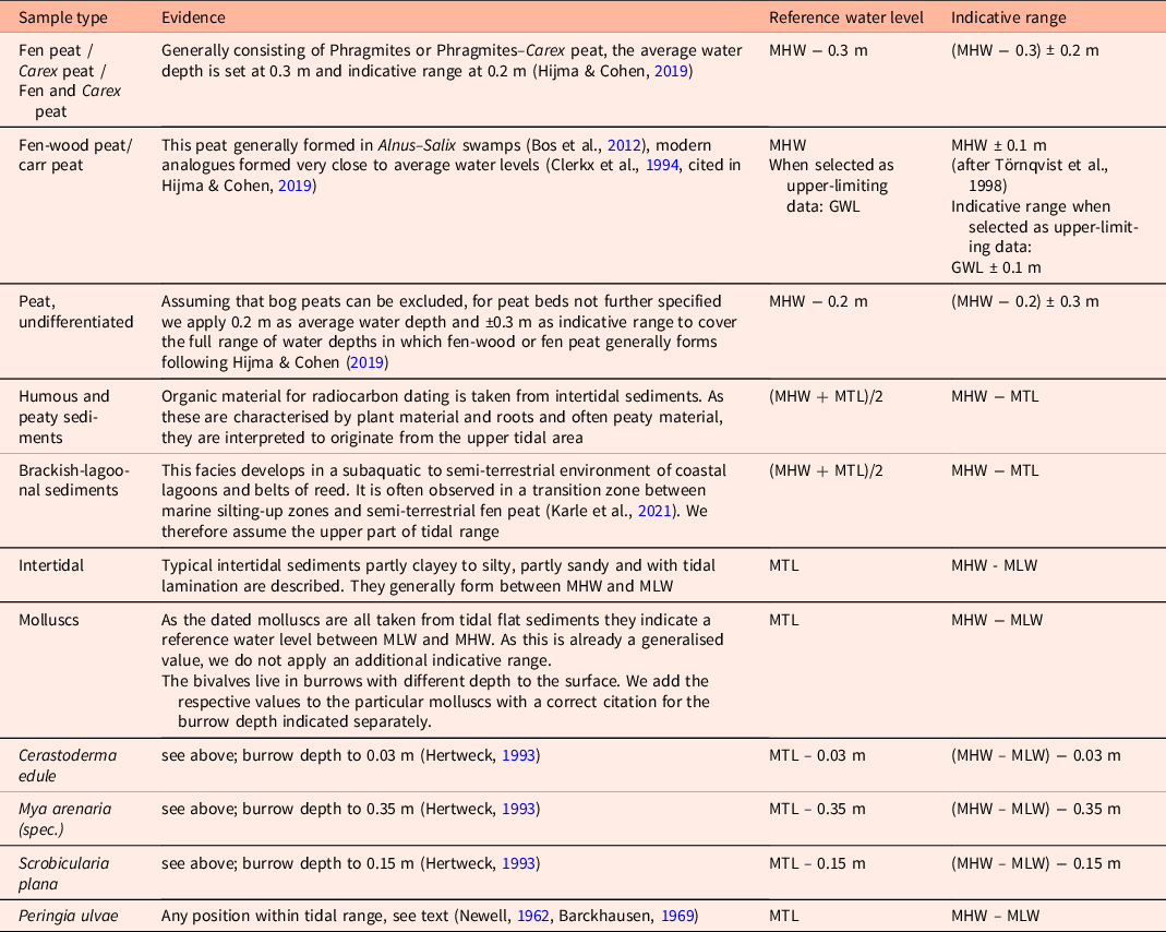
The 14C age determinations (bulk) were performed by the LBEG and the Poznań Radiocarbon Laboratory, Poland (Table 1). The results were calibrated using CALIB (Version 8.2), IntCal20 and Marine20 (Reimer et al., Reference Reimer, Austin, Bard, Bayliss, Blackwell, Bronk Ramsey, Butzin, Cheng, Edwards, Friedrich, Grootes, Guilderson, Hajdas, Heaton, Hogg, Hughen, Kromer, Manning, Muscheler, Palmer, Pearson, van der Plicht, Reimer, Richards, Scott, Southon, Turney, Wacker, Adolphi, Büntgen, Capano, Fahrni, Fogtmann-Schulz, Friedrich, Köhler, Kudsk, Miyake, Olsen, Reinig, Sakamoto, Sookdeo and Talamo2020).
Table 1. Summary of the indicative meanings of the different sample types in the Langeoog area. The samples providing upper-limiting data are collected from fen-wood peat or carr peat. For those the reference water level is the ground water level (GWL) and additionally specified in the table. In the Langeoog back-barrier area, MHW is at 1.42 m MSL, MTL is at 0.10 m. For more detailed information on tide levels see the Supplementary Material available online at https://doi.org/10.1017/njg.2021.11
All ages from shells were derived from articulated in situ specimens. The specimens of the gastropod Peringia ulvae were collected from the stratigraphically important layer ‘Hydrobien-Schichten’ of Langeoog (Barckhausen, Reference Barckhausen1969). According to measurements of Enters et al. (Reference Enters, Haynert, Wehrmann, Freund and Schlütz2021) the delta R value for reservoir correction of ages originating from in situ shell material was applied with −85 ± 17.
All radiocarbon data are plotted with the 2σ error (Figs 3, 4, 5 and 6).
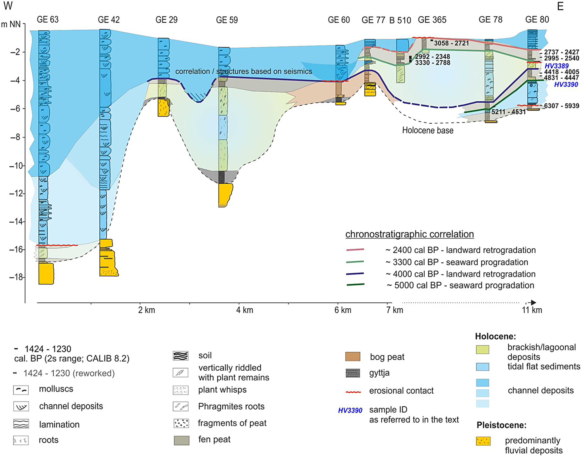
Fig. 3. West–east cross section ‘Stüversledge’ and chronostratigraphic correlations. For the osition of the cross section see Fig. 2.


Fig. 6. The complete dataset for the Langeoog area.
(vii) OSL data
The OSL age determination was performed by the OSL laboratory at the Department of Geography of the University of Liverpool, UK. Samples were treated following the preparation procedures for silt-sized quartz grains samples for multiple-grain aliquots (Mauz et al., Reference Mauz, Bode, Mainz, Blanchard, Hilger, Dikau and Zöller2002). Although ‘variable bleaching rules’ in tidal-flat sub-environments have to be considered, OSL dates from tidally deposited sediments show consistent chronologies (Mauz et al., Reference Mauz, Baeteman, Bungenstock and Plater2010; Zhang et al., Reference Zhang, Tsukamoto, Grube and Frechen2014). For a detailed description of the samples used see Bungenstock (Reference Bungenstock2006) and Mauz & Bungenstock (Reference Mauz and Bungenstock2007).
Indicative meaning of the peat
Age data were taken from basal as well as from intercalated fen peats.
Studies on coastal landscape reconstruction, sea-level and peat data show height differences of up to several metres for peat of the same age. This demonstrates the independence of several basal peat formations from sea level due to local hydrography, which has been described before by Jelgersma (Reference Jelgersma1961), Lange & Menke (Reference Lange and Menke1967), Van de Plassche (Reference Van de Plassche1982), Wolters et al., (Reference Wolters, Zeiler and Bungenstock2010), Hepp et al., (Reference Hepp, Romero, Mörz, De Pol-Holz and Hebbeln2019) and Karle et al., (Reference Karle, Bungenstock and Wehrmann2021) for the North Sea. As no plant macro-remains or pollen data are provided for the peat samples, which could prove a marine influence, age data of the basal peat beds are tested for their reliability in terms of sea-level data by their position in cross sections (see Figs 3, 4 and 5) and in the age–depth diagram (Fig. 6). Based on this analysis the basal peat beds are classified either as sea-level index points or as upper-limiting data points. The top of a basal peat is often a sea-level index point when non-erosively overlain by brackish–marine sediments (Hijma et al., Reference Hijma, Engelhart, Törnqvist, Horton, Hu, Hill, Shennan, Long and Horton2015), which is not the case in the available dataset of this study.
Fen peats are nourished by groundwater, which, consequently, influences the peat’s growth. Groundwater level, in turn, is often controlled by sea level in coastal areas and it is generally accepted that basal peat within coastal zones starts forming at local MHW level (Van de Plassche, Reference Van de Plassche1982; Hijma & Cohen, Reference Hijma and Cohen2019). The better the peat is characterised for its plant association, the more precisely its relation to MHW can be defined, as shown by Den Held et al., (Reference Den Held, Schmitz and Van Wirdum1992), Clerkx et al., (Reference Clerkx, Van Dort and Hommel1994), Berendsen et al., (Reference Berendsen, Makaske, van de Plassche, van Ree, Das, van Dongen, Ploumen and Schoenmakers2007) and Bos et al., (Reference Bos, Busschers and Hoek2012). The different kinds of fen peats of the presented database are listed in Table 1, with their respective relation to MHW as derived from literature.
The same relation applies for intercalated peats. Certainly, for intercalated peats compaction of underlying sediments is a crucial issue to consider. Thus, intercalated peats provide additional information (Engelhart & Horton, Reference Engelhart and Horton2012), but have to be carefully evaluated for their deposition in situ, their stratigraphic meaning (e.g. reworked or not) and compaction of underlying sediments.
Indicative meaning of the mollusc samples
Only articulated shells in living position were dated. These are Cerastoderma edule (Linnaeus 1758), Scrobicularia plana (da Costa 1778), Mya arenaria (Linnaeus 1758) and Mya truncata (Linnaeus 1758), all sampled from intertidal sediments from outcrops on Langeoog island. They are plotted with the full tidal range as error envelope (s. Table 1). Furthermore, it is worth considering that the associated burrows reach different depths: Cerastoderma edule burrows down to 3 cm (Klausnitzer Reference Klausnitzer2019), Scrobicularia plana to 15 cm (Hertweck, Reference Hertweck1993) and Mya arenaria to 35 cm (Hertweck, Reference Hertweck1993). Therefore, they refer to mean tidal level (with the full tidal range as indicative range) minus the respecitve burrow depth (see Table 1).
Additionally, four radiocarbon datings of the gastropod Periniga ulvae (formerly Hydrobia ulvae) are available. Peringia ulvae reaches its maximum density at approximately mid-tide level, but it also floats during high tide and burrows in the sand during low tide (Newell, Reference Newell1962). Peringia ulvae can reach densities of over 370,000 individuals per square metre (Schückel et al., Reference Schückel, Beck and Kröncke2013). At the former southern rim of Langeoog island, a layer of Peringia ulvae stretches ∼10 km in the N–S direction and over 3 km in the W–E direction. It is described as stratigraphic key layer, the so-called Hydrobienschicht (Hydrobia layer) marking a former island position (Barckhausen, Reference Barckhausen1969). Following Barckhausen (Reference Barckhausen1969) it developed at the southern rim of the former island Langeoog in shallow and quiet water with plenty of algae food supply for Peringia ulvae. Maybe it was even protected by surrounding sand bars, which prevented uplift and transport of the snale during high water. However, Peringia ulvae accumulated there and obviously did not drift away. The Perinigia ulvae ages sampled from the ‘Hydrobienschicht’ also refer to mean tide level with the full tidal range as indicative range.
Indicative meaning of the samples dated by OSL
The OSL samples are plotted with their original depth plus the full tidal range as error range, as no indicative meaning other than ‘deposited within tidal range’ can be deduced. This is in contrast to Mauz & Bungenstock (Reference Mauz and Bungenstock2007) who suggest an indicative meaning based on assumptions of the position of the samples in the upper, middle or lower third of the tidal range based on the macroscopic facies description, but without robust microfauna analyses. The OSL samples are defined as sea-level index points, as MSL cannot lie lower or higher than the full error range of these samples.
Uncertainties
All age data are plotted with the 2σ error. For calculation of the vertical error we follow the HOLSEA workflow. All uncertainties are filled in the 77-field sea-level spreadsheet provided by Khan et al., (Reference Khan, Horton, Engelhart, Rovere, Vacchi, Ashe, Törnqvist, Dutton, Hijma and Shennan2019) (see Supplementary Material available online at https://doi.org/10.1017/njg.2021.11). For more information about the now standardised uncertainties to be regarded, see Hijma et al., (Reference Hijma, Engelhart, Törnqvist, Horton, Hu, Hill, Shennan, Long and Horton2015) and Khan et al., (Reference Khan, Horton, Engelhart, Rovere, Vacchi, Ashe, Törnqvist, Dutton, Hijma and Shennan2019).
Compaction
Compaction as a term used in the following comprises auto-compaction and compression. Auto-compaction is a non-mechanical diagenetic process including structural collapse, biological decay and chemical alteration of organic matter. Compression mainly depends on the overburden. It concerns all kinds of unconsolidated deposits.
Bennema et al., (Reference Bennema, Geuze, Smits and Wiggers1954) describe peat compaction of maximal 85–90%; Kaye & Barghoorn (Reference Kaye and Barghoorn1964) observe peat compaction of 80–90% for samples from the North American coast. In these cases, a correction factor for decompaction of at least 5 has to be applied. Denys & Baeteman (Reference Denys and Baeteman1995) assume an average compaction of 50% (correction factor 2). Roeleveld & Gotjé (Reference Roeleveld and Gotjé1993) apply a minimum and maximum correction factor of 0 and 3, which is modified by Van de Plassche et al., (Reference Van de Plassche, Bohncke, Makaske and Van der Plicht2005) and Berendsen et al., (Reference Berendsen, Makaske, van de Plassche, van Ree, Das, van Dongen, Ploumen and Schoenmakers2007) to a correction factor of 1.5 for the base of the dated sample and a correction factor of 2.5 for the top of the dated sample. Although Van de Plassche et al., (Reference Van de Plassche, Makaske, Hoek, Konert and van der Plicht2010) state that Berendsen et al., (Reference Berendsen, Makaske, van de Plassche, van Ree, Das, van Dongen, Ploumen and Schoenmakers2007) used 2.5 and 3.5 as correction factor instead of 1.5 and 2.5 as written in the text, it is not clear which correction factor is the correct one and whether the 2.5 and 3.5 factor had also been used before by Van de Plassche et al., (Reference Van de Plassche, Bohncke, Makaske and Van der Plicht2005), which was cited by Berendsen et al., (Reference Berendsen, Makaske, van de Plassche, van Ree, Das, van Dongen, Ploumen and Schoenmakers2007). However, Khan et al., (Reference Khan, Horton, Engelhart, Rovere, Vacchi, Ashe, Törnqvist, Dutton, Hijma and Shennan2019) suggest applying a factor of 2.5 for the correction of the sample thickness referring to Van de Plassche et al. (Reference Van de Plassche, Bohncke, Makaske and Van der Plicht2005), Van Asselen (Reference Van Asselen2011) and Hijma et al., (Reference Hijma, Engelhart, Törnqvist, Horton, Hu, Hill, Shennan, Long and Horton2015).
Smith et al., (Reference Smith, Wells, Mighall, Cullingford, Holloway, Dawson and Brooks2003) and Lloyd et al., (Reference Lloyd, Zong, Fish and Innes2013) estimate peat compaction underneath clastic sediments by 40–68%, which is a factor between 1.66 and 3.125. If the thickness of the clastic overburden exceeds 2.5 m, they assume that the compaction of the underlying peat has been completed before the deposition of another regressive layer such as an intercalated peat bed.
For fine-grained sediments which suffered post-depositional compression, the model for decompaction published by Paul & Barras (Reference Paul and Barras1998) gives an average depth correction of 5–10% of the layer thickness.
These approaches are useful when the local data densities allow detailed observation of compaction rates; unfortunately, this is often not the case. Any correction would then lead to inaccuracies and eventually even falsify the original data further (Edwards, Reference Edwards2006; Engelhart & Horton, Reference Engelhart and Horton2012). Thus, the data are classified into base-of-basal, basal and intercalated peat in the age–depth diagram to take the different compaction potential into account for the interpretation of the sea-level data (Shennan et al., Reference Shennan, Lambeck, Flather, Horton, McArthur, Innes, Lloyd, Rutherford and Wingfield2000; Horton & Shennan, Reference Horton and Shennan2009; Engelhart & Horton, Reference Engelhart and Horton2012). Additionally, after tackling the best data for the drawing of the RSL curve, we measured the distances of the compaction-prone samples to the consolidated Pleistocene basement and to the centre line of our RSL curve as an approach to suggest a factor of decompaction for our study area.
Ideally, the base of basal peat is positioned directly, or only few centimetres, above the Pleistocene basement. For the dataset presented here, no data point applies for these prerequisites. The base-of-basal peat data are therefore defined as such if positioned a maximum of 0.20 m above the Pleistocene, to differentiate them from other basal peat data in our dataset, which are positioned 0.45–3.41 m above the Pleistocene. The samples defined as base of basal peat data vary between 5 and 10 cm thickness. Of course, they also comprise a compaction uncertainty. Nevertheless, they provide the best data of the dataset available for the Langeoog area.
Sea-level index points
The indicative meaning of every data point has been calculated following the principles of the HOLSEA workflow (Khan et al, Reference Khan, Horton, Engelhart, Rovere, Vacchi, Ashe, Törnqvist, Dutton, Hijma and Shennan2019; see Table 1; Supplementary Material available online at https://doi.org/10.1017/njg.2021.11). Sea-level index points and lower- and upper-limiting data are differentiated and are plotted in an age–depth diagram (Fig. 6). The sea-level index points were evaluated as such following three criteria: (1) the original sample description; (2) the correlation within cross sections (Figs 3, 4 and 5) and seismic profiles to evaluate the data for compaction and whether they can be correlated over several hundred metres to exclude local reworking and transport (see Bungenstock & Schäfer, Reference Bungenstock and Schäfer2009); and (3) the position in the age–depth diagram (Fig. 6).
Results and interpretation
Progradation and retrogradation: signals in the sedimentary record
In Table 2, all samples with their 2σ age range, sample depth and indicative meaning for RSL are listed, together with the core they are taken from, to give a general overview and to better identify the samples in the cross sections (Figs 3, 4 and 5). For details of facies description and error ranges see the Supplementary Material available online at https://doi.org/10.1017/njg.2021.11.
Table 2. List of all available data for the Langeoog area as plotted in Figure 6. The samples analysed are legacy data from different projects and not taken originally for sea-level research. Therefore, many of them are not taken at transgressive contacts, but in the middle or in the upper or lower parts of a peat layer. Lab numbers of the samples evaluated as reliable for the RSL curve are marked in boldface. The oldest sea-level index point, which is used for the curve although it is compaction-prone, is underlined. The 2σ age range is listed in the fourth column. The peat data are calibrated with Calib 8.2, Intcal20 (Reimer et al., Reference Reimer, Austin, Bard, Bayliss, Blackwell, Bronk Ramsey, Butzin, Cheng, Edwards, Friedrich, Grootes, Guilderson, Hajdas, Heaton, Hogg, Hughen, Kromer, Manning, Muscheler, Palmer, Pearson, van der Plicht, Reimer, Richards, Scott, Southon, Turney, Wacker, Adolphi, Büntgen, Capano, Fahrni, Fogtmann-Schulz, Friedrich, Köhler, Kudsk, Miyake, Olsen, Reinig, Sakamoto, Sookdeo and Talamo2020), the mollusc data are calibrated with Calib 8.2, Marine 20 (Reimer et al., Reference Reimer, Austin, Bard, Bayliss, Blackwell, Bronk Ramsey, Butzin, Cheng, Edwards, Friedrich, Grootes, Guilderson, Hajdas, Heaton, Hogg, Hughen, Kromer, Manning, Muscheler, Palmer, Pearson, van der Plicht, Reimer, Richards, Scott, Southon, Turney, Wacker, Adolphi, Büntgen, Capano, Fahrni, Fogtmann-Schulz, Friedrich, Köhler, Kudsk, Miyake, Olsen, Reinig, Sakamoto, Sookdeo and Talamo2020). Delta R −85 ± 17 (Enters et al., Reference Enters, Haynert, Wehrmann, Freund and Schlütz2021) and the OSL data are corrected to BP. Dat. (third) column specifies the dating method, SLIP stands for sea-level index point, nd stands for not defined, n/a stands for not applicable. Further details about the facies, calculation of errors and the indicative meaning are listed in the Supplementary Material available online at https://doi.org/10.1017/njg.2021.11

In the study area intercalated peat beds, which are representative for a local seaward progradation of the coastline, form after the deceleration of RSL ∼6000 cal BP. The first one dates to 5600 cal BP, the last one ends at 2500 cal BP (Figs 3 and 4). For a short period from 4000 to 3800 cal BP, no intercalated peat beds are documented in the study area (Fig. 6). The reason for this transgressional phase is not clear. The RSL for Langeoog shows neither an acceleration, nor an increase in energy, which would be suggested by erosional contacts, sand layers or even shell layers but which are not documented in the cores (see Figs 3 and 4). However, after ∼2500 cal BP, intertidal marine deposition dominates throughout the study area in parts with an erosional contact on top of the underlying brackish–lagoonal sediments and peats (Figs 3 and 4).
Langeoog RSL curve
The age–depth diagram in Figure 6 shows the entire dataset plotted with its indicative meaning for MSL as reference water level and the vertical and horizontal 2σ error. Additionally, for every sample the depth from the midpoint to the consolidated substrate (Pleistocene) is plotted.
Out of the 68 sea-level data, 30 are used as sea-level index points. Four of those are of relatively strong quality in terms of vertical uncertainty ranges. The oldest sea-level index point is compaction-prone but the best one available for that time, five data points are lower-limiting data, at least two data points (probably five, see discussion about the peat data in BLB2) are upper-limiting data. Most rejected data were rejected due to strong compaction (Table 2; Supplementary Material available online at https://doi.org/10.1017/njg.2021.11). The 2 σ error boxes of the chosen samples are connected to depict the RSL error envelope (Fig. 6). All chosen samples are marked in Table 2 and plotted in Figures 3, 4 and 5.
For ∼6700 to 3000 cal BP, four sea-level index points are derived from the base of the peat layer with a depth between 0 and 0.20 m to the consolidated substrate (Pleistocene). The error envelope for ∼6700 to 3000 cal BP is depicted by connecting the error boxes of these four sea-level index points. The error envelope is complemented for the period since ∼7200 cal BP by the best sea-level index point available, which is a sample taken from a basal peat with 0.62 m depth to the Pleistocene. Further supporting data, which plot within the error envelope, are derived from four basal peat data with 0.45–0.94 m depth to the Pleistocene. Additionally, it should be mentioned that five samples from intercalated peats with 2.30 m, 2.48 m and unknown depth to the Pleistocene also plot in the error envelope. The RSL curve starts with a rise of 0.40 m per century and decelerates to 0.16 m per century since ∼6000 cal BP.
For 3000 cal BP to Recent, 18 SLIPs are available, with a wide vertical uncertainty range. For the upper boundary of the error envelope the lowest error boxes, and for the lower boundary of the error envelope the uppermost error boxes, are connected. As there is a wide uncertainty range, a reliable course of RSL is hard to estimate. Nevertheless, a deceleration of RSL seems to be apparent since ∼2500 cal BP.
Estimation of compaction on basal and intercalated peat beds
As the dataset comprises base-of-basal peat data on which the RSL curve is based, the compaction effect of all other data becomes obvious and is, as expected, dependent on the thickness and the material of the deposits underneath the respective sample. In Figure 6 the distance of the midpoint of every sample to the Pleistocene is plotted. The compaction of every sample is estimated by simply measuring the vertical distance from the midpoint of the respective sample to the centre line of the RSL curve. In Tables 3 and 4 the factor necessary to decompact a sample to plot it on the centre line of our RSL curve is calculated. While the average decompaction factor for basal peats is calculated with 2.29, the average decompaction factor for intercalated peats is 1.67. The basal peats HV4728, HV4729 and HV4263 – all taken from core GE176 (Fig. 4) – are excluded as outliers as their decompaction factors far exceed the factors of the other samples. This means, when decompacting the basal peat data with the factor 2.29 and the intercalated peat data with 1.67, all data (except the above-mentioned outliers) plot at least within the error band.
Table 3. Reconstructed factors of decompaction for basal peat samples. The average value is 2.29, excluding the three high values from core GE176 (HV4728, HV4729, HV4263; see Fig. 4). HV4263 is clearly an outlier (see Fig. 6)

Table 4. Reconstructed factors of decompaction for intercalated peat samples; the average value is 1.67

A compaction-corrected RSL curve resulting from applying the calculated decompaction factor of 2.29 on the base of basal peat data is plotted in Figure 6 as red dotted line.
Discussion
Compaction of basal peats and sediments below intercalated peat samples
In Figure 6 the depth to consolidated substrate for the sea-level index points from 7200 to 3000 cal BP is depicted in the data error boxes. In Tables 3 and 4 the compaction rates and the respective factors of decompaction are calculated based on the dataset, that allows for reconstructing the RSL curve, with data lacking between 6000 and 3000 cal BP resulting in a straight line in between the chosen data (Fig. 6). For the RSL curve, especially the samples lying not more than 20 cm above the Pleistocene deposits have been used. Most other samples show a clear impact of compaction with up to 55% (HV4731 from core GE184, Fig. 4)), although there are some exceptions, such as HV3389 and 3390 from core GE80 (see Fig. 3) with only 5% and 16% of compaction (Table 4), or the peat samples from BLB2 lying in the upper part of the RSL error envelope, although they are taken from 0.47–0.94 m above the Pleistocene deposits (Fig. 6). However, it cannot be excluded that the samples of BLB2 are upper-limiting data as no botanical analysis is available. The only thing that can be stated here is that the cores are from the mainland part of the area.
While the compaction of basal peat ranges from 43 to 98% – with most samples lying between 50 and 70% – the compaction of the material (peat and sediments) underlying the intercalated peat samples ranges from 5 to 55% – with most samples lying between 35 and 55% – independent of the existence and thickness of a basal peat underneath. One explanation for this difference is that in general the intercalated peat beds are much thinner than the basal peat beds in the study area.
Especially for the basal peat samples, the compaction varies strongly in the presented dataset. For core GE176 the lower and upper extreme value of compaction is documented: 43% in the upper part of the peat layer and 98% in the lower part. The given core description as well as the geographical position of the cross section (Fig. 4) cannot explain the extreme range of compaction rates of the lower part of the basal peats. This attests to the often incalculable effect of compaction. Nevertheless, for the remaining dataset of 10 samples a decompaction rate from 1.76 to 2.89 with an average of 2.29 was calculated, which provides at least an estimate for a correction of compaction of basal peats for the study area.
The average decompaction rate of the material underneath the intercalated peat samples is less than that of the basal peats and is calculated at 1.67, although the thickness to the Pleistocene is generally higher than that of the basal peat samples. Furthermore, the thickness of the basal peat in the cores from which intercalated peat samples are taken does not seem to directly influence the amount of compaction. The variation of the decompaction factor of intercalated peat samples is independent of both the general thickness of the underlying material and the thickness of basal peat in the geological record. This supports the assumption that the main compaction process of the basal peat ended before the intercalated peat bed developed.
This agrees in principle with the findings of Smith et al. (Reference Smith, Wells, Mighall, Cullingford, Holloway, Dawson and Brooks2003) and Lloyd et al. (Reference Lloyd, Zong, Fish and Innes2013). They come to the conclusion that the compaction of the underlying peat was completed before the deposition of another regressive layer, such as an intercalated peat bed. The prerequisite for this assumption is that the thickness of the clastic overburden exceeds 2.5 m (Smith et al., Reference Smith, Wells, Mighall, Cullingford, Holloway, Dawson and Brooks2003; Lloyd et al., Reference Lloyd, Zong, Fish and Innes2013). The overburden observed in our cores in many cases is significantly less than 2.50 m, with values of for example 0.55 m and 1.40 m. What cannot completely be excluded here is erosion of formerly deposited material, although this is not indicated by the core descriptions.
As the dataset for the RSL curve is not complete and data from ∼6000 cal BP and 3000 cal BP had to be connected by a straight line instead of a possibly more curved shape, we consider our decompaction estimates as first-order approximations which likely represent minimum values in most cases. We assume that the calculated decompaction factors are underestimated for most cases and just give a minimum value. Nevertheless, the decompaction necessary for basal peats is higher than that for samples taken from intercalated peats.
Sea-level-independent asynchronous landscape development along the coast
When comparing Holocene sedimentary records of the coastal areas between the Ems and Elbe estuaries, a different number of intercalated peat beds is noted: only one peat bed in the Stade–Buxtehude area adjacent to the Elbe estuary and up to seven intercalated peat beds in the Weser estuary (Streif, Reference Streif2004). Moreover, these intercalated peat layers show inconsistent chronologies. Following the cross sections published by Streif (Reference Streif2004), only the uppermost peat bed has a consistent age of ∼2000 BP (calendar years, not calibrated) along the coast, although the calibrated dataset presented here for Langeoog suggests the growth of the uppermost peat for ∼3000 cal BP. Raised bog on top of intercalated fen peat is documented for the Jade Bay and the Ems estuary only.
We assume that the development of peat beds is driven by local sediment supply probably varying in the different tidal basins. Another reason for asynchronous development that needs to be mentioned here could be the flood basin effect (Van de Plassche, Reference Van de Plassche1982; Kiden et al., Reference Kiden, Makaske and van de Plassche2008; Vis et al., Reference Vis, Cohe, Westerhoff, Ten Veen, Hijma., Van der Spek, Vos, Shennan, Long and Horton2015; Hijma & Cohen, Reference Hijma and Cohen2019), which is a drop of high-water level and tidal range when a tidal basin is closed off from the open sea. Behind this closing shore the influence of the tides decreases and peat starts to grow, indeed typically over large areas. Thus, across-basin occurring peat does not necessarily indicate falling sea level but locally falling high-water level in an individual tidal basin. The Flemish and Zeeland coasts have undergone several switches from closed to open basins during the Holocene (Vos & Van Heeringen, Reference Vos and van Heeringen1997; Baeteman, Reference Baeteman1999). Also, from Flanders, Zeeland and Holland it is known that a very slowly rising sea level supports a closing coast due to onshore sediment transport (e.g. Beets & van der Spek, Reference Beets and van der Spek2000). For the East Frisian coast, the barrier island chain is assumed to have existed since ∼7 ka (Flemming & Davis, Reference Flemming and Davis1994), but details of its mid–late Holocene development are yet to be investigated. Anyway, in contrast to the Netherlands coast, for the East Frisian Peninsula no closing coast has been documented so far. According to historical maps (e.g. Le Coq, Reference LeCoq1805; Homeier, Reference Homeier1964), the East Frisian island chain modified its shape over time, in general with islands becoming longer and thereby narrowing tidal inlets in between. However, these maps apply for the time when dikes had been built and made the coastline of the mainland static.
Notwithstanding the lack of details, for the mid–late Holocene it is documented that the mainland-shoreline prograded seawards and that mires have developed over wide areas since then (Streif, Reference Streif2004; Karle et al., Reference Karle, Bungenstock and Wehrmann2021). Furthermore, changes in strength and frequency of storm surges are crucial for the progradation or retrogradation of the coastline by erosion or redistribution of sediment. Baeteman (Reference Baeteman2005) and Karle et al. (Reference Karle, Bungenstock and Wehrmann2021) show drainage and compaction of marshes and peatlands initiated by the incision of channels and subsequent inundation. This results in an apparent acceleration of sea-level rise but is in fact a local relative water-level rise due to compaction effects (cf. Long et al., Reference Long, Waller and Stupples2006).
For the Langeoog tidal basin it is assumed that sediment supply is the most relevant trigger for coastal progradation and peat development because tidal channels and creeks are important sediment suppliers and drainage networks for changing the depositional environment as shown by Baeteman (Reference Baeteman, Thoen, Borger, de Kraker, Soens, Tys, Vervaet and Weerts2013). Therefore, intercalated peats mostly reflect local sedimentary processes or perhaps local changes of water level in case of changes in tide levels, but do not generally represent changes of RSL trends. For the study area, intercalated peat beds are documented from ∼5600 cal BP to ∼2700 cal BP. What can be assessed here is a short phase of transgression from ∼4000 cal BP to ∼3800 cal BP but without any hints of sea-level acceleration or single events documented in the RSL curve and sedimentological record.
To determine whether this is just a local phenomenon for the back-barrier of Langeoog or whether it has a regional meaning for e.g. the entire East Frisian coast, other back-barrier areas will have to be analysed in the same detail (Bungenstock & Weerts, Reference Bungenstock and Weerts2012). Furthermore, high-precision RSL indicators such as derived from the transgressional contact of thin basal peat beds or from a Foraminifera transfer function (Scheder et al., Reference Scheder, Frenzel, Bungenstock, Engel, Brueckner and Pint2019) are needed to better quantify changes in RSL if existent.
Comparison with other regional RSL curves and assumptions on glacial isostatic adjustment (GIA)
RSL curves standardised following the HOLSEA sea-level protocol (Khan et al., Reference Khan, Horton, Engelhart, Rovere, Vacchi, Ashe, Törnqvist, Dutton, Hijma and Shennan2019) are best for a direct comparison, so that artificial differences due to different approaches can be prevented. We therefore plot the MSL curve for the western Netherlands by Hijma & Cohen (Reference Hijma and Cohen2019), who work with their own data and integrate the data by van de Plassche et al. (Reference Van de Plassche, Makaske, Hoek, Konert and van der Plicht2010). Hijma & Cohen (Reference Hijma and Cohen2019) used a combination of base-of-basal peat and top-of-basal peat data, which are non-erosively overlain by tidal deposits, with most data only 5 cm above the unconsolidated substrate (Fig. 7).
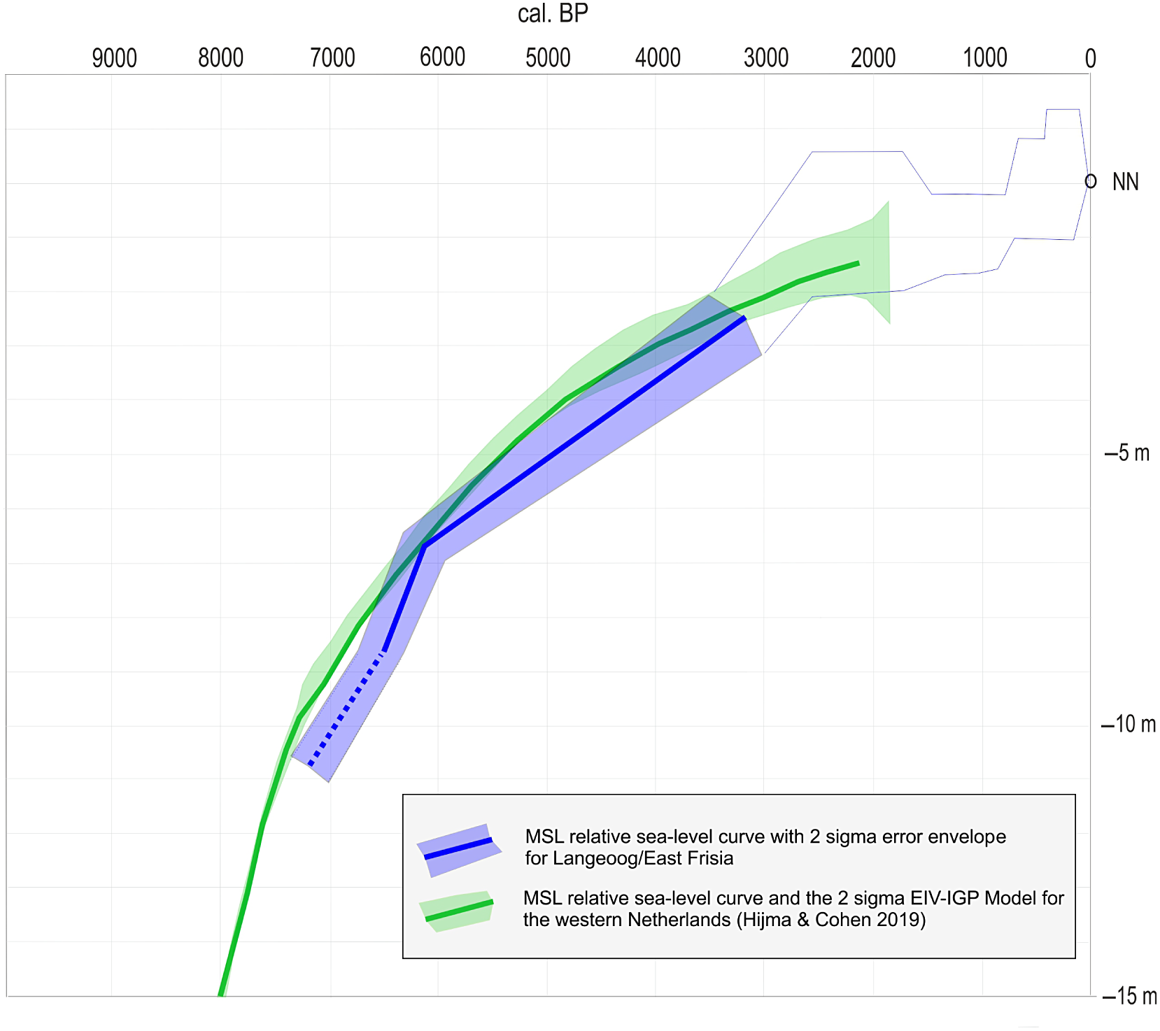
Fig. 7. The decompacted Langeoog RSL curve (see Fig. 6) and the RSL curve for the Western Netherlands by Hijma & Cohen (Reference Hijma and Cohen2019). For locations see Figure 1.
The RSL curve for Langeoog lies below the curve for the western Netherlands, nevertheless with overlapping error envelopes, while before 6000 cal BP it seems to diverge (Fig. 7), indicating that the main GIA effect is apparent before ∼6000 cal BP. The offset of up to 0.80 m between 6000 and 3000 cal BP is probably mainly due to the straight course of the Langeoog curve during this timespan. More data would probably allow to scetch its course more curved and the two curves would be even closer. The calculated decompaction factors for this study had to be adjusted (accelerated). Plotting RSL curves from other coastal areas along the southern North Sea coast without correcting the data for their respective indicative meaning as provided by the HOLSEA sea-level protocol (Hijma et al., Reference Hijma, Engelhart, Törnqvist, Horton, Hu, Hill, Shennan, Long and Horton2015; Khan et al., Reference Khan, Horton, Engelhart, Rovere, Vacchi, Ashe, Törnqvist, Dutton, Hijma and Shennan2019) carries the risk of depicting the offset effect of tide data, e.g. mean high-water level, rather than the effect of GIA. The published GIA model predictions for the southern North Sea (Vink et al., Reference Vink, Steffen, Reinhardt and Kaufmann2007) are based on previously published sea-level data, not applying the later-developed standardisation provided by Khan et al. (Reference Khan, Horton, Engelhart, Rovere, Vacchi, Ashe, Törnqvist, Dutton, Hijma and Shennan2019). Comparing the predicted RSL curve for Wangerooge, which is ∼20 km east of Langeoog, and the predicted RSL curve for the western Netherlands shows an offset of 3 m at 6000 cal BP and 1.5 m at 3000 cal BP. This is much higher than that between the RSL curve of Langeoog and the RSL curve for the western Netherlands by Hijma & Cohen (Reference Hijma and Cohen2019) with an offset in decimetre range and overlapping error envelopes.
Conclusions
The revised RSL curve for Langeoog, complemented with additional data, is significantly different from that previously published by Bungenstock & Schäfer (Reference Bungenstock and Schäfer2009), as phases of still-stand, deceleration or strong acceleration of RSL since 6000 cal BP cannot be proven by the evaluated dataset presented here.
The subordinate progradational and retrogradational signals in the Langeoog area are supposed to mirror local effects, which are expected to vary along the German coastline as documented by Streif (Reference Streif2004) and Karle et al., (Reference Karle, Bungenstock and Wehrmann2021). Therefore, intercalated peat data as indicators for changes of RSL in the sense of a slowdown of sea-level rise or even a still-stand are questionable. Nevertheless, they provide important information for local coastal progradation, which is suspected to be asynchronous along the German North Sea coast. For the study area, a short phase of transgression from ∼4000 cal BP to ∼3800 cal BP can be assessed, but without any hints on sea-level acceleration or single events. The evaluation of sea-level index points from adjacent tidal basins will provide more information for a reliable review of the stratigraphic meaning of the intercalated peat beds along the East Frisian coast.
Overall, compaction is, as expected, a difficult factor to calculate. However, our data show that compaction of basal peats is higher than that of the sediments underlying the samples from intercalated peat beds. The necessary factors of decompaction calculated here, at 2.29 for basal peats and 1.67 for samples from intercalated peats, are probably underestimated, as they were calculated for the centre line of the presented RSL curve, which is unnaturally straight due to the few data points.
The comparison with the RSL curve for the western Netherlands shows that the Langeoog curve lies below the western Netherlands curve. In the part older than 6000 cal BP, the Langeoog RSL curve diverges from the western Netherlands curve, whereas since ∼6000 cal BP the Langeoog curve is close to the RSL curve for the western Netherlands, with the Langeoog curve lying up to 0.80 m below. This difference is probably mainly due to the lack of data of the Langeoog curve and its resulting straight shape in contrast to the curved shape of the western Netherlands curve. Most probably, this difference would diminish with a better dataset for Langeoog. However, in any case this means a smaller impact of GIA for the time since 6000 cal BP than modelled so far.
The dataset presented here was not originally taken for the purpose of sea-level research and no material is left to do more detailed analysis. Overall, the Langeoog dataset is not of the quality of those used in other sea-level papers (Meijles et al., Reference Meijles, Kiden, Streurman, Van der Plicht, Vos, Gehrels and Kopp2018; Hijma & Cohen, Reference Hijma and Cohen2019) in terms of suitability and precision with ideally transgressive contacts on thin basal peat beds. Nevertheless, the dataset contributes a step forward towards sea-level research accordant with the new sea-level protocol (Khan et al., Reference Khan, Horton, Engelhart, Rovere, Vacchi, Ashe, Törnqvist, Dutton, Hijma and Shennan2019), providing comparability and a base for further work along the German North Sea coast. In a next step, SLIPs for further tidal basins along the southern North Sea should be analysed and evaluated.
Supplementary material
Supplementary material is available online at https://doi.org/10.1017/njg.2021.11.
Acknowledgements
This contribution was greatly improved by the extremely constructive reviews of an anonymous reviewer, Patrick Kiden and Robin Edwards. A warm thanks goes to Barbara Mauz for discussion and improving the English wording. We thank the State Office for Mining and Geology of Lower Saxony (LBEG) for providing basic digital data for the Langeoog study (Scha 279/18-1). We thank Jobst Barckhausen for detailed geological background information about the Langeoog area. Our gratitude goes to all the students and colleagues who participated in the fieldwork. This publication is dedicated in memoriam to Henk Weerts, who encouraged the main author to continue with sea-level studies.
This paper is a contribution to the IGCP project 639 ‘Sea level change from minutes to millennia.’


 Open access