


1. Introduction
Optimal investment theory is an important topic in quantitative risk management and involves determining how to allocate capital among available securities in order to maximize the expected return for a given level of risk or minimize the associated risk for a given level of return. Markowitz [Reference Markowitz13] proposed the first quantitative method for determining the optimal portfolio based on minimizing the portfolio variance for a given expectation, called mean-variance principle. In classical optimal investment theory, the distribution obeyed by the data is usually assumed to be known or an empirical distribution function is used instead of the unknown distribution, whereas in practice, the distribution obeyed by the data cannot be determined if the complete data is not available or if a small sample of data is obtained and an empirical distribution function cannot be used. This resulted in other samples performing poorly.
Motivated by this, distributionally robust optimization (DRO) has emerged as a paradigm aimed at finding a solution that is protected against sampling errors [Reference Delage and Ye6]. It seeks for a solution that performs the best with respect to the most adversarial distribution from a set of distributions, known as ambiguity set. The DRO identifies the most adversarial distribution, the worst-case distribution, from an ambiguity set, and makes an optimal decision, the optimal portfolio, which minimizes the cost induced by the worst-case distribution. The choice of a proper ambiguity set is crucial in DRO. Such DRO problem and its robust decision have been verified to exhibit some desirable properties such as finite-sample guarantee and computational tractability, which are in sharp contract with the classic stochastic optimization problem. Hence, DRO has been widely applied in data-driven problems arising from many operations research and machine learning applications. Among others, in portfolio selection, Blanchet et al. [Reference Blanchet, Chen and Zhou3] consider DRO based on mean-variance principle. The same principle is also used in Calafiore and Ghaoui [Reference Calafiore and Ghaoui4], Zhu et al. [Reference Zhu, Zhang and Ye22] and Popescu [Reference Popescu17], in which a linear-chance-constrained problem, a minimax regret objective and a portfolio optimization problem are considered, respectively. However, mean-variance principle has been criticized for that its measure of risk, variance, is not a monotone measure. Shadwick and Keating [Reference Shadwick and Keating18] introduced the Omega ratio to analyze information on the distribution of potential returns. Essentially, it is the ratio of the upside of an investment to the downside. Omega ratio has been verified to provide a new perspective in the performance evaluation of hedge funds [Reference Shadwick and Keating18] and build as a useful measure [Reference Bertrand and Prigent1]. Therefore, in this paper, we focus on DRO based on the mean-Omega ratio principle in portfolio selection. Specifically, we first calculate the worst-case Omega ratio from the ambiguity set and then find the optimal portoflio, which minimizes the worst-case Omega ratio. While the current paper focuses on mean-Omega ratio principles, we should point out that recently several other works have explored other measures such as mean-VaR and mean-CVaR in distributionally robust portfolio selection (see [Reference Kang, Li, Li and Zhu11, Reference Kang, Zhao and Sun12] and the references therein).
In addition to the principle employed in DRO, the choice of a proper ambiguity set is crucial in DRO. In particular, one common way of defining the set  ${\cal F}$ is through specifying the moments of the distribution (see, e.g., [Reference Bertsimas, Doan, Natarajan and Teo2, Reference Delage and Ye6, Reference Natarajan, Sim and Uichanco15, Reference Popescu17, Reference Wiesemann, Kuhn and Sim21]); DRO problems based on moments information has been proved to have a tractable form in applications. So we will first consider the worst-case Omega ratio based on the mean-variance information. Motivated by recent advances in data-driven DRO problem, we also consider that the uncertainty set is the Wasserstein ball centred at the empirical distribution. The Wasserstein ball that is centered at the empirical distribution has become popular as it can make full use of the data, and this ambiguity set has become an attractive ambiguity set adopted in DRO. To solve a DRO problem, identifying the most adversarial distribution, the worst-case distribution, from an ambiguity set is essential. We first study the worst-case distribution and calculate its Omega ratio. The worst-case Omega ratio is calculated under mean-variance uncertainty set and mean-Wasserstein uncertainty set, respectively. With aid of the projection result of the two ambiguity sets, we apply the results in the portfolio selection.
The rest of the paper is organized as follows. Section 2 presents the definition of the Omega ratio, gives explicit expression of the worst-case Omega ratio under mean-variance uncertainty set and aims to tackle the worst-case Omega ratio under mean-Wasserstein uncertainty set. Section 3 applies the worst-case Omega ratio under mean-variance uncertainty set and mean-Wasserstein uncertainty set to the portfolio. In Section 4, we present the simulation and empirical results derived from portfolios comprised of our strategies, comparing them to those of various alternative models.
Throughout the paper, let  $d \in \mathbb{N}$ and $\mathbb{R}^d$ be the d-dimensional Euclidean space. Let $\mathcal{P}(\mathbb{R}^d)$ be the set of all distributions on $\mathbb{R}^d$ and denote $\mathcal{P}_p(\mathbb{R}^d)$ by the subset of $\mathcal{P}(\mathbb{R}^d)$ with finite pth moment for $p \in [1,\infty)$. For a random variable (vector) $\mathbf X\in \mathcal{P}(\mathbb{R}^d)$, denote $\mathbb{E}[{\mathbf X}]$ by the mean (vector) of the random variable (vector) $\mathbf X$. For a law-invariantFootnote 1 real-valued mapping ρ on $\mathcal{P}(\mathbb{R}^d)$, the notation $\rho^{F}({\mathbf X})$ means the value of $\rho({\mathbf X})$, where ${\mathbf X}$ has the distribution F, and we omit F for simplicity. Furthermore, we denote by $x_+=\max(0,x)$ and $x_-=\max(0,-x)$.
2. Worst-case Omega ratio
In this section, we only discuss the case of d = 1. The case of d > 1 is discussed in Section 3, where the corresponding portfolio selection problem is investigated. One popular measure of investment performance in finance is Omega ratio introduced by Shadwick and Keating [Reference Shadwick and Keating18]: the ratio of the upside of an investment to the downside.
Definition 2.1. (Shadwick and Keating [Reference Shadwick and Keating18])
For a payoff X with distribution F and a sure payoff c, Omega ratio is defined as
 \begin{equation*}
\Omega_{X}(c):=\frac{\mathbb{E}\left[(X-c)_{+}\right]}{\mathbb{E}\left[(c-X)_{+}\right]}.
\end{equation*}
\begin{equation*}
\Omega_{X}(c):=\frac{\mathbb{E}\left[(X-c)_{+}\right]}{\mathbb{E}\left[(c-X)_{+}\right]}.
\end{equation*}2.1. Mean-variance uncertainty set
We assume that the distribution of X lies in a distribution set where first and second moments are fixed. Based on this assumption, we consider the following DRO problem for Omega ratio:
 \begin{equation}
\underline{\Omega}_{X}(c,\mu,\sigma) = \inf_{F\in \mathcal{S}_{1}} \Omega_{X}^{F}(c),
\qquad
\overline{\Omega}_{X}(c,\mu,\sigma) = \sup_{F \in \mathcal S_{1}} \Omega_{X}^{F}(c),
\end{equation}
\begin{equation}
\underline{\Omega}_{X}(c,\mu,\sigma) = \inf_{F\in \mathcal{S}_{1}} \Omega_{X}^{F}(c),
\qquad
\overline{\Omega}_{X}(c,\mu,\sigma) = \sup_{F \in \mathcal S_{1}} \Omega_{X}^{F}(c),
\end{equation}where
 \begin{align}
\mathcal S_{1}:={\cal S}(\mu,\sigma) =\left\{F\in\mathcal{P}_2(\mathbb{R}): \int_{-\infty}^\infty x\, \mathrm{d}F(x)=\mu, \int_{-\infty}^\infty x^2\, \mathrm{d}F(x)=\mu^2+\sigma^2 \right\},
\end{align}
\begin{align}
\mathcal S_{1}:={\cal S}(\mu,\sigma) =\left\{F\in\mathcal{P}_2(\mathbb{R}): \int_{-\infty}^\infty x\, \mathrm{d}F(x)=\mu, \int_{-\infty}^\infty x^2\, \mathrm{d}F(x)=\mu^2+\sigma^2 \right\},
\end{align}and  $ \Omega_{X}^{F}(c)$ represents the Omega ratio that is calculated under the constraint that the distribution of X is F. The following theorem gives the explicit solutions of the optimization problem (1).
Theorem 2.2. Given  $\mu\in\mathbb{R}$ and σ > 0, we have
 \begin{align}
\underline{\Omega}_{X}(c,\mu,\sigma)=
\begin{cases}
0, & \mu \lt c, \\
\frac{\sqrt{1+S^2}+S}{\sqrt{1+S^2}-S}, & \mu \geqslant c ,
\end{cases}
\end{align}
\begin{align}
\underline{\Omega}_{X}(c,\mu,\sigma)=
\begin{cases}
0, & \mu \lt c, \\
\frac{\sqrt{1+S^2}+S}{\sqrt{1+S^2}-S}, & \mu \geqslant c ,
\end{cases}
\end{align}and
 \begin{align}
\overline{\Omega}_{X}(c,\mu,\sigma)=
\begin{cases}
\frac{\sqrt{1+S^2}+S}{\sqrt{1+S^2}-S}, & \mu \lt c, \\
\infty, & \mu \geqslant c,
\end{cases}
\end{align}
\begin{align}
\overline{\Omega}_{X}(c,\mu,\sigma)=
\begin{cases}
\frac{\sqrt{1+S^2}+S}{\sqrt{1+S^2}-S}, & \mu \lt c, \\
\infty, & \mu \geqslant c,
\end{cases}
\end{align}where  $S= \frac{\mu - c}{\sigma}$.
We first present a lemma from [Reference Jagannathan10], which is subsequently used in the proof of Theorem 2.2.
Lemma 2.3. Given  $\mu\in\mathbb{R}$ and σ > 0, we have
 \begin{equation*}
\max_{F \in \mathcal{S}_{1}} \mathbb{E}^F[(X-c)_+]=\frac{1}{2}\left[\sqrt{\sigma^2+(\mu-c)^2}+\mu-c\right],
\end{equation*}
\begin{equation*}
\max_{F \in \mathcal{S}_{1}} \mathbb{E}^F[(X-c)_+]=\frac{1}{2}\left[\sqrt{\sigma^2+(\mu-c)^2}+\mu-c\right],
\end{equation*}where  $\mathcal S_1$ is defined by Eq. (2).
Proof of Theorem 2.2
Since  $\mathbb{E}^F[X-c]=\mathbb{E}^F[(X-c)_+]-\mathbb{E}^F[(X-c)_{-}]=\mathbb{E}^F[(X-c)_+]-\mathbb{E}^F[(c-X)_{+}]$, the Omega function can be rewritten as
 \begin{align}
\Omega_{X}^F(c)=\frac{\mathbb{E}^F[(X-c)_+]}{\mathbb{E}^F[(c-X)_+]} =\frac{\mathbb{E}^F[(X-c)_+]}{\mathbb{E}^F[(X-c)_+]-\mathbb{E}^F[(X-c)]}
=\left\{{1-\frac{\mathbb{E}^F[X]-c}{\mathbb{E}^F[(X-c)_+]}} \right\}^{-1}.
\end{align}
\begin{align}
\Omega_{X}^F(c)=\frac{\mathbb{E}^F[(X-c)_+]}{\mathbb{E}^F[(c-X)_+]} =\frac{\mathbb{E}^F[(X-c)_+]}{\mathbb{E}^F[(X-c)_+]-\mathbb{E}^F[(X-c)]}
=\left\{{1-\frac{\mathbb{E}^F[X]-c}{\mathbb{E}^F[(X-c)_+]}} \right\}^{-1}.
\end{align} We first consider the case of  $\underline{\Omega}_{X}(c,\mu,\sigma)$. If $\mu \geqslant c$, then we have
 \begin{align*}
\underline{\Omega}_{X}(c,\mu,\sigma)&=\inf_{F\in \mathcal{S}_{1}} \Omega_{X}^{F}(c)
=\inf_{F\in \mathcal{S}_{1}}\left\{1-\frac{\mathbb{E}^F[X]-c}{\mathbb{E}^F[(X-c)_+]}\right\}^{-1}\\
&=\left\{1-\frac{\mu-c}{\max_{F\in\mathcal{S}_{1}}\{\mathbb{E}^F[(X-c)_+]\}}\right\}^{-1}\\
&=\left\{1-\frac{\mu-c}
{\frac12 [\sqrt{\sigma^2+(\mu-c)^2}+\mu-c]}\right\}^{-1}\\
&=\frac{\sqrt{1+S^2}+S}{\sqrt{1+S^2}-S},
\end{align*}
\begin{align*}
\underline{\Omega}_{X}(c,\mu,\sigma)&=\inf_{F\in \mathcal{S}_{1}} \Omega_{X}^{F}(c)
=\inf_{F\in \mathcal{S}_{1}}\left\{1-\frac{\mathbb{E}^F[X]-c}{\mathbb{E}^F[(X-c)_+]}\right\}^{-1}\\
&=\left\{1-\frac{\mu-c}{\max_{F\in\mathcal{S}_{1}}\{\mathbb{E}^F[(X-c)_+]\}}\right\}^{-1}\\
&=\left\{1-\frac{\mu-c}
{\frac12 [\sqrt{\sigma^2+(\mu-c)^2}+\mu-c]}\right\}^{-1}\\
&=\frac{\sqrt{1+S^2}+S}{\sqrt{1+S^2}-S},
\end{align*}where the second and fourth equalities follow from Eq. (5) and Lemma 2.3, respectively. If  $\mu \lt c$, define a discrete random variable as follows:
 \begin{equation}
X_\alpha=\left\{
\begin{aligned}
\mu-\sigma\sqrt{\frac{1-\alpha}{\alpha}},\quad & \textrm{with probability}\ \alpha, \\
\mu+\sigma\sqrt{\frac{\alpha}{1-\alpha}}, \quad & \textrm{with probability}\ 1-\alpha.
\end{aligned}
\right.
\end{equation}
\begin{equation}
X_\alpha=\left\{
\begin{aligned}
\mu-\sigma\sqrt{\frac{1-\alpha}{\alpha}},\quad & \textrm{with probability}\ \alpha, \\
\mu+\sigma\sqrt{\frac{\alpha}{1-\alpha}}, \quad & \textrm{with probability}\ 1-\alpha.
\end{aligned}
\right.
\end{equation} Let  $\alpha \lt \frac{(\mu-c)^2}{\sigma^2+(\mu-c)^2}$. One can check that $\mathbb{E}[X_\alpha]=\mu$, $\mathrm{Var}(X_\alpha)=\sigma^2$, which implies that $F_{X_\alpha}\in\mathcal S_1$. Also noting that $X_\alpha \lt c$ almost surely, we have
 \begin{equation*}
0\leqslant \underline{\Omega}_{X}(c,\mu,\sigma)\leqslant \Omega_{X_\alpha}(c)=0.
\end{equation*}
\begin{equation*}
0\leqslant \underline{\Omega}_{X}(c,\mu,\sigma)\leqslant \Omega_{X_\alpha}(c)=0.
\end{equation*} Hence, we conclude that  $\underline{\Omega}_{X}(c,\mu,\sigma)=0$ for $\mu \lt c$. This completes the proof of Eq. (3).
Next, we consider the case of  $\overline{\Omega}_{X}(c,\mu,\sigma)$. If $\mu\leqslant c$, then we have
 \begin{align*}
\overline{\Omega}_{X}(c,\mu,\sigma)&=\sup_{F\in \mathcal{S}_{1}} \Omega_{X}^{F}(c)
=\sup_{F\in \mathcal{S}_{1}}\left\{1-\frac{\mathbb{E}^F[X]-c}{\mathbb{E}^F[(X-c)_+]}\right\}^{-1}\\
&=\left\{1+\frac{c-\mu}{\max_{F\in\mathcal{S}_{1}}\{\mathbb{E}^F[(X-c)_+]\}}\right\}^{-1}\\
&=\left\{1+\frac{c-\mu}
{\frac12 [\sqrt{\sigma^2+(\mu-c)^2}+\mu-c]}\right\}^{-1}\\
&=\frac{\sqrt{1+S^2}+S}{\sqrt{1+S^2}-S},
\end{align*}
\begin{align*}
\overline{\Omega}_{X}(c,\mu,\sigma)&=\sup_{F\in \mathcal{S}_{1}} \Omega_{X}^{F}(c)
=\sup_{F\in \mathcal{S}_{1}}\left\{1-\frac{\mathbb{E}^F[X]-c}{\mathbb{E}^F[(X-c)_+]}\right\}^{-1}\\
&=\left\{1+\frac{c-\mu}{\max_{F\in\mathcal{S}_{1}}\{\mathbb{E}^F[(X-c)_+]\}}\right\}^{-1}\\
&=\left\{1+\frac{c-\mu}
{\frac12 [\sqrt{\sigma^2+(\mu-c)^2}+\mu-c]}\right\}^{-1}\\
&=\frac{\sqrt{1+S^2}+S}{\sqrt{1+S^2}-S},
\end{align*}where the second and fourth equalities follow from Eq. (5) and Lemma 2.3, respectively. If  $\mu \gt c$, recall the definition of Xα in Eq. (6). Let $\alpha \gt \frac{(\mu-c)^2}{\sigma^2+(\mu-c)^2}$. One can check that $\mathbb{E}[X_\alpha]=\mu$, ${\mathrm{Var}}(X_\alpha)=\sigma^2$, which implies that $F_{X_\alpha}\in\mathcal S_1$. Also noting that $X_\alpha \gt c$ almost surely, we have
 \begin{equation*}
\overline{\Omega}_{X}(c,\mu,\sigma)\geqslant \Omega_{X_\alpha}(c)=+\infty.
\end{equation*}
\begin{equation*}
\overline{\Omega}_{X}(c,\mu,\sigma)\geqslant \Omega_{X_\alpha}(c)=+\infty.
\end{equation*} Hence, we have  $\underline{\Omega}_{X}(c,\mu,\sigma)=0$ for $\mu \gt c$. This completes the proof of (4).
Remark 1. The slope of a straight line tangent to the efficient frontier, consisting of both risky and risk-free assets, is called the Sharpe ratio [Reference Sharpe19]. That is, for a random variable X with mean µ and standard deviation σ, Sharpe ratio is defined as  $ S_{X} = \frac{\mathbb{E}[X] - r_0}{\sqrt{\mathrm{Var}(X)}}$, where $\mathrm{Var}$ represents the variance and r 0 is a reference return rate, typically taken as the risk-free return rate. Theorem 2.2 implies that the upper and lower bounds of the Omega ratio can be obtained from a given Sharpe ratio, which is included by the uncertainty set (2). Observing the forms of Eqs. (3) and (4), we find that the robust value increases with the given Sharpe ratio.
2.2. Mean-Wasserstein uncertainty set
In this section, we present the worst-case Omega ratio based on Wasserstein uncertainty set. We first give the definition of Wasserstein Distance from [Reference Villani20].
Definition 2.5. (Wasserstein Distance)
The p-Wasserstein distance  $W_{p}(G_1,G_2)$ between $G_1,G_2 \in \mathcal{P}_p(\mathbb{R}^d)$ is defined by
 \begin{align*}
W_{p}(G_1,G_2) &:=\\
&\inf_{\pi \in \mathcal{P}_p(\mathbb{R}^d \times \mathbb{R}^d)} \left\{\left( \int_{\mathbb{R}^d \times \mathbb{R}^d} \left\lVert x-y \right\rVert ^p \pi({\rm d}x,{\rm d}y) \right)^{\frac{1}{p}} \Big|{\pi \in \mathcal{P}_p(\mathbb{R}^d \times \mathbb{R}^d) \ \ s.t.\ \ \atop \pi( \cdot \times \mathbb{R}^d)=G_1,\ \pi(\mathbb{R}^d \times \cdot)=G_2} \right\},
\end{align*}
\begin{align*}
W_{p}(G_1,G_2) &:=\\
&\inf_{\pi \in \mathcal{P}_p(\mathbb{R}^d \times \mathbb{R}^d)} \left\{\left( \int_{\mathbb{R}^d \times \mathbb{R}^d} \left\lVert x-y \right\rVert ^p \pi({\rm d}x,{\rm d}y) \right)^{\frac{1}{p}} \Big|{\pi \in \mathcal{P}_p(\mathbb{R}^d \times \mathbb{R}^d) \ \ s.t.\ \ \atop \pi( \cdot \times \mathbb{R}^d)=G_1,\ \pi(\mathbb{R}^d \times \cdot)=G_2} \right\},
\end{align*}where  $\left\lVert \cdot\right\rVert $ is a norm on $\mathbb{R}^d$, whose dual norm is defined as $\|y\|_*:=\sup_{\left\lVert x\right\rVert \leqslant 1}x^\top y$ for $ y \in \mathbb{R}^d$.
The Wasserstein distance is a natural way to compare two distributions when one is obtained from the other by perturbation. For a fixed  $F \in \mathcal{P}_p(\mathbb{R}^d)$ and ɛ > 0, the Wasserstein ball centered on F is defined as follows:
 \begin{align*}
\mathscr B^p_{\varepsilon}(F) :=\left\{G \in {\cal P}_p(\mathbb{R}^d) \big| W_{p}(G,F) \leqslant \varepsilon\right\}.
\end{align*}
\begin{align*}
\mathscr B^p_{\varepsilon}(F) :=\left\{G \in {\cal P}_p(\mathbb{R}^d) \big| W_{p}(G,F) \leqslant \varepsilon\right\}.
\end{align*} For d = 1, we are interested in the worst-case Omega ratio in scenarios where the expected return is greater than the risk-free return, that is,  $\mathbb{E}[X] \geqslant c$, where c is the risk-free return. Hence, we consider the worst-case Omega ratio under the mean and p-Wasserstein uncertainty set:
 \begin{equation}
\underline{\Omega}_{X}^F(c,\mu,\varepsilon)=\inf_{G \in {\mathcal S}_{2}} \Omega_{X}^G(c), \quad
\end{equation}
\begin{equation}
\underline{\Omega}_{X}^F(c,\mu,\varepsilon)=\inf_{G \in {\mathcal S}_{2}} \Omega_{X}^G(c), \quad
\end{equation}where  $F \in \mathcal{P}_p(\mathbb{R})$,
 \begin{equation*}
{\mathcal S}_{2}:={{\cal S}_{p,\varepsilon}(\mu,F)}=\left\{G \in \mathscr B^p_{\varepsilon}(F) \big| \int x \,{\rm d}G(x)=\mu \right\}
\end{equation*}
\begin{equation*}
{\mathcal S}_{2}:={{\cal S}_{p,\varepsilon}(\mu,F)}=\left\{G \in \mathscr B^p_{\varepsilon}(F) \big| \int x \,{\rm d}G(x)=\mu \right\}
\end{equation*}and  $\Omega_{X}^G(c) $ represents the Omega ratio that is calculated under the constraint that the distribution of X is G.
We turn to the main result of this section, which indicates that the explicit solution of problem (7) is obtained for p = 1, and we simplify problem (7) for p > 1.
Theorem 2.6. Given c, µ, ɛ > 0,  $p \in [1,\infty)$ and $F \in \mathcal{P}_p(\mathbb{R})$, assume $\mu \geqslant c$. Let $\underline{\Omega}_{X}^F(c,\mu,\varepsilon)$ be the optimal value of problem (7) for a given distribution F, µF denote the random variable’s mean under the distribution F. We have the following results.
(i) For p = 1, $\mu_F^{c_+}:=\mathbb{E}^F[(X-c)_+]$, then
where\begin{equation*}
\underline{\Omega}_{X}^F(c,\mu,\varepsilon)=\left\{
\begin{aligned}
&1, & \textrm{if}\ \mu \in \mathcal{A}_1\cup \mathcal{B}_1, \\
&\left[1-\frac{2(\mu-c)}{\mu-\mu_F+\varepsilon}\right]^{-1}, & \textrm{if}\ \mu \in \mathcal{A}_2\cup \mathcal{B}_2,
\end{aligned}
\right.
\end{equation*}$\mathcal{A}_1=\{\mu:\mu \gt \mu_F-\mu_F^{c_+}, \mu \gt \mu_F-2\mu_F^{c_+}+\varepsilon\},$ $\mathcal{A}_2=\{\mu:\mu \gt \mu_F-\mu_F^{c_+}, \mu \leqslant \mu_F-2\mu_F^{c_+}+\varepsilon\}$, $\mathcal{B}_1=\{\mu:\mu \leqslant \mu_F-\mu_F^{c_+}, \mu \lt \mu_F-\varepsilon\}$ and $\mathcal{B}_2=\{\mu:\mu \leqslant \mu_F-\mu_F^{c_+}, \mu \geqslant \mu_F-\varepsilon\}$.
$\mu_F^{c_+}:=\mathbb{E}^F[(X-c)_+]$, then
where\begin{equation*}
\underline{\Omega}_{X}^F(c,\mu,\varepsilon)=\left\{
\begin{aligned}
&1, & \textrm{if}\ \mu \in \mathcal{A}_1\cup \mathcal{B}_1, \\
&\left[1-\frac{2(\mu-c)}{\mu-\mu_F+\varepsilon}\right]^{-1}, & \textrm{if}\ \mu \in \mathcal{A}_2\cup \mathcal{B}_2,
\end{aligned}
\right.
\end{equation*}$\mathcal{A}_1=\{\mu:\mu \gt \mu_F-\mu_F^{c_+}, \mu \gt \mu_F-2\mu_F^{c_+}+\varepsilon\},$ $\mathcal{A}_2=\{\mu:\mu \gt \mu_F-\mu_F^{c_+}, \mu \leqslant \mu_F-2\mu_F^{c_+}+\varepsilon\}$, $\mathcal{B}_1=\{\mu:\mu \leqslant \mu_F-\mu_F^{c_+}, \mu \lt \mu_F-\varepsilon\}$ and $\mathcal{B}_2=\{\mu:\mu \leqslant \mu_F-\mu_F^{c_+}, \mu \geqslant \mu_F-\varepsilon\}$.(i) Otherwise, for p > 1, we have
where\begin{equation*}
\underline{\Omega}_{X}^F(c,\mu,\varepsilon)=\left( 1- \frac{\mu-c}{T(\mu)}\right)^{-1},
\end{equation*}and\begin{equation*}
\begin{aligned}
T(\mu) := \inf_{\lambda \geqslant 0 , \gamma \in \mathbb{R}} \left\{\lambda \varepsilon^p +\gamma (\mu - \mu_F) + |\gamma| \left(1- \frac{1}{p}\right) \left( \frac{|\gamma |}{\lambda p}\right)^{\frac{1}{p-1}} + \mathbb{E}^F [ (X-c_1(\lambda,\gamma))_+]\right\} \\
\end{aligned}
\end{equation*}\begin{equation*}
\begin{aligned}
c_1(\lambda,\gamma) := c+\left(1-\frac{1}{p}\right) \left[ \left( \frac{|\gamma |}{\lambda p}\right)^{\frac{1}{p-1}} |\gamma| - \left( \frac{|1-\gamma |}{\lambda p}\right)^{\frac{1}{p-1}}|1-\gamma| \right]. \\
\end{aligned}
\end{equation*}


To simplify problem (7), we need to utilize the following lemma, the proof of which is directly derived from Theorem 1 of [Reference Gao and Kleywegt8].
Lemma 2.7. For  $p \in [1,\infty)$, $ F \in \mathcal{P}_p(\mathbb{R}),$ $\mu \in \mathbb{R}$, ɛ > 0 and $\Psi:\mathbb{R}\to\mathbb{R}$, we have
 \begin{equation*}
\begin{aligned}
\sup_{G \in {\mathcal S}_{2}} \int_{\mathbb{R}} \Psi(\xi)\,{\rm d}G( \xi) =\inf_{\lambda \geqslant 0, \gamma \in \mathbb{R}} \left\{\lambda \varepsilon^p +\int_{\mathbb{R}} \sup_{\xi \in \mathbb{R}} [\Psi(\xi)-\gamma \xi-\lambda | \xi-\zeta | ^p ]\, {\rm d}F( \zeta) +\gamma \mu \right\}.
\end{aligned}
\end{equation*}
\begin{equation*}
\begin{aligned}
\sup_{G \in {\mathcal S}_{2}} \int_{\mathbb{R}} \Psi(\xi)\,{\rm d}G( \xi) =\inf_{\lambda \geqslant 0, \gamma \in \mathbb{R}} \left\{\lambda \varepsilon^p +\int_{\mathbb{R}} \sup_{\xi \in \mathbb{R}} [\Psi(\xi)-\gamma \xi-\lambda | \xi-\zeta | ^p ]\, {\rm d}F( \zeta) +\gamma \mu \right\}.
\end{aligned}
\end{equation*}Proof of Theorem 2.6
We know that if  $\mathbb{E}^G[X]=\mu$, Omega ratio can be expressed as
 \begin{equation*}
\Omega_{X}^G(c)=\frac{\mathbb{E}^G [(X-c)_+]}{\mathbb{E} ^G[(c-X)_+]}=\left\{{1- \frac{\mu-c}{\mathbb{E}^G [( X-c)_+]}}\right\}^{-1}.
\end{equation*}
\begin{equation*}
\Omega_{X}^G(c)=\frac{\mathbb{E}^G [(X-c)_+]}{\mathbb{E} ^G[(c-X)_+]}=\left\{{1- \frac{\mu-c}{\mathbb{E}^G [( X-c)_+]}}\right\}^{-1}.
\end{equation*} Denote  $T(\mu)= \sup_{G \in {\mathcal S}_{2}} \mathbb{E}^G [(X-c)_+]$, for $\mu \geqslant c$, we can obtain that
 \begin{equation*}
\inf_{G \in {\mathcal S}_{2}} \frac{\mu-c}{\mathbb{E}^G [(X-c)_+]} =\frac{\mu-c}{T(\mu)}.
\end{equation*}
\begin{equation*}
\inf_{G \in {\mathcal S}_{2}} \frac{\mu-c}{\mathbb{E}^G [(X-c)_+]} =\frac{\mu-c}{T(\mu)}.
\end{equation*}Hence, problem (7) can be reduced as follow:
 \begin{align*}
\underline{\Omega}_{X}(\mu,c,\varepsilon)&=\inf_{G \in {\mathcal S}_{2}} \Omega_{X}^G(c) = \inf_{G \in {\mathcal S}_{2}} \left\{{1- \frac{\mu-c}{\mathbb{E}^G [(X-c)_+]}}\right\}^{-1}\\
&=\left\{1-\inf_{G \in {\mathcal S}_{2}} {\frac{\mu-c}{\mathbb{E}^G [(X-c)_+]}}\right\}^{-1}\\
&=\left\{1-\frac{\mu-c}{T(\mu)}\right\}^{-1}\\
&=\frac{T(\mu)}{T(\mu)-(\mu-c)}.
\end{align*}
\begin{align*}
\underline{\Omega}_{X}(\mu,c,\varepsilon)&=\inf_{G \in {\mathcal S}_{2}} \Omega_{X}^G(c) = \inf_{G \in {\mathcal S}_{2}} \left\{{1- \frac{\mu-c}{\mathbb{E}^G [(X-c)_+]}}\right\}^{-1}\\
&=\left\{1-\inf_{G \in {\mathcal S}_{2}} {\frac{\mu-c}{\mathbb{E}^G [(X-c)_+]}}\right\}^{-1}\\
&=\left\{1-\frac{\mu-c}{T(\mu)}\right\}^{-1}\\
&=\frac{T(\mu)}{T(\mu)-(\mu-c)}.
\end{align*}Applying Lemma 2.7, denote by
 \begin{equation*}
H_{\lambda,\gamma}(y)= \sup_{x \in \mathbb{R}} \{(x-c)_+ - \gamma x -\lambda |x-y|^p \},
\end{equation*}
\begin{equation*}
H_{\lambda,\gamma}(y)= \sup_{x \in \mathbb{R}} \{(x-c)_+ - \gamma x -\lambda |x-y|^p \},
\end{equation*}  $T(\mu)$ can be reformulated as
 \begin{equation}
T(\mu)=\sup_{G \in {\mathcal S}_{2}} \mathbb{E}^G[(X-c)_+]=\inf_{\lambda \geqslant 0, \gamma \in \mathbb{R}} \left\{\lambda \varepsilon^p + \mathbb{E}^F \left[ H_{\lambda,\gamma}(Y) \right]+\gamma \mu \right\}.
\end{equation}
\begin{equation}
T(\mu)=\sup_{G \in {\mathcal S}_{2}} \mathbb{E}^G[(X-c)_+]=\inf_{\lambda \geqslant 0, \gamma \in \mathbb{R}} \left\{\lambda \varepsilon^p + \mathbb{E}^F \left[ H_{\lambda,\gamma}(Y) \right]+\gamma \mu \right\}.
\end{equation} To simplify  $T(\mu)$, we calculate the RHS of Eq. (8) in the following steps.
1. Calculate
$H_{\lambda,\gamma}(y)$.Let
$h_y(x)=(x-c)_+ - \gamma x -\lambda |x-y|^p$. For $x \in \mathbb{R}\backslash\{c,y\}$, the derivative of $h_y(x)$ with respect to x is
\begin{equation*}
\begin{aligned}
\frac{\partial h_y(x)}{\partial x} &=I(x \gt c)-\gamma - \text{sgn}(x-y) \lambda p |x-y|^{p-1}. \\
\end{aligned}
\end{equation*}To calculate the maximum of
$h_y(x)$, we consider the case of p = 1 and p > 1, respectively.(i) If p = 1, for
$x \in \mathbb{R}\backslash\{c,y\}$, the derivative of $h_y(x)$ with respect to x can be written as
\begin{equation*}
\begin{aligned}
\frac{\partial h_y(x)}{\partial x}
&=
\begin{cases}
1-\gamma - \lambda , & x \gt \max\{c,y\}, \\
I(x \gt c)-\gamma - \text{sgn}(x-y) \lambda, &x \in (\min\{c,y\},\max\{c,y\}), \\
-\gamma +\lambda , & x \lt \min\{c,y\}. \\
\end{cases}
\end{aligned}
\end{equation*}In the case of
$\lambda \geqslant \frac{1}{2}$ and $1-\lambda \leqslant \gamma \leqslant \lambda$, if $\frac{\partial h_y(x)}{\partial x} \geqslant 0 $ for $x \lt \min\{c,y\}$ and $\frac{\partial h_y(x)}{\partial x} \leqslant 0 $ for $x \gt \max\{c,y\}$, then the maximizer to $h_y(x)$ lies in the interval $[\min\{c,y\},\max\{c,y\}]$. If y < c, as $\frac{\partial h_y(x)}{\partial x} \leqslant 0 $ for $x \in (y,c)$, the maximizer to $h_y(x)$ is $x^*=y$ and $h_y(y)=-\gamma y$. If $y \geqslant c$, as $\frac{\partial h_y(x)}{\partial x} \geqslant 0 $ for $x \in (c,y)$, the maximizer to $h_y(x)$ is $x^*=c$ and $h_y(c)=-\lambda y+(\lambda-\gamma)c$. Otherwise, it can be verified that
\begin{equation*}\sup_{x \in \mathbb{R}}h_y(x)=\max\{\lim_{x \to \infty}h_y(x),\lim_{x \to -\infty}h_y(x)\}=\infty.\end{equation*}In summary, in the case of p = 1, if
$\lambda \geqslant \frac{1}{2}$ and $1-\lambda \leqslant \gamma \leqslant \lambda$, the value of $H_{\lambda, \gamma}(y)$ is
otherwise, the value of\begin{equation*}
H_{\lambda, \gamma}(y)=\sup_{x \in \mathbb{R}} h_y(x)=
\begin{cases}
-\gamma y, & y \lt c,\\
-\lambda y+(\lambda-\gamma)c, & y \geqslant c; \\
\end{cases}
\end{equation*}$H_{\lambda, \gamma}(y)$ is $\infty$.(ii) If p > 1, for y < c, we have
\begin{equation*}
\begin{aligned}
\frac{\partial h_y(x)}{\partial x}
&=
\begin{cases}
1-\gamma - \lambda p |x-y|^{p-1}, & x \gt c, \\
-\gamma - \lambda p |x-y|^{p-1}, &x \in (y,c), \\
-\gamma +\lambda p |x-y|^{p-1}, & x \lt y. \\
\end{cases}
\end{aligned}
\end{equation*}Conversely, for
$y \geqslant c$, then
\begin{equation*}
\begin{aligned}
\frac{\partial h_y(x)}{\partial x}
&=
\begin{cases}
1-\gamma - \lambda p |x-y|^{p-1}, & x \gt y, \\
1-\gamma + \lambda p |x-y|^{p-1}, &x \in (c,y), \\
-\gamma +\lambda p |x-y|^{p-1}, & x \lt c. \\
\end{cases}
\end{aligned}
\end{equation*}Therefore, it is necessary to discuss the classification of γ. For
$\gamma \leqslant 0$, we consider the following three cases.(a) For
$y \lt c-\left(\frac{1-\gamma}{\lambda p}\right)^{\frac{1}{p-1}}$, solving $\frac{\partial h_y(x)}{\partial x} \gt 0$ yields $x \lt y+\left(\frac{-\gamma}{\lambda p}\right)^{\frac{1}{p-1}}$ and solving $\frac{\partial h_y(x)}{\partial x}\leqslant 0$ yields $x\geqslant y+\left(\frac{-\gamma}{\lambda p}\right)^{\frac{1}{p-1}}$. As a result, the maximizer to $h_y(x)$ is $x_1^*=y+\left(\frac{-\gamma}{\lambda p}\right)^{\frac{1}{p-1}}$ and
\begin{equation*}
h_y(x_1^*)=-\gamma y - \gamma \left(1- \frac{1}{p}\right) \left( \frac{- \gamma}{\lambda p}\right)^{\frac{1}{p-1}}.
\end{equation*}(b) For
$c-\left(\frac{1-\gamma}{\lambda p}\right)^{\frac{1}{p-1}} \leqslant y \leqslant c-\left(\frac{-\gamma}{\lambda p}\right)^{\frac{1}{p-1}}$, we find that $\frac{\partial h_y(x)}{\partial x} \gt 0$ in the cases that $x \lt y+\left(\frac{-\gamma}{\lambda p}\right)^{\frac{1}{p-1}}$ or $c \lt x \lt y+\left(\frac{1-\gamma}{\lambda p}\right)^{\frac{1}{p-1}}$ and $\frac{\partial h_y(x)}{\partial x}\leqslant 0$ in the cases that $y+\left(\frac{-\gamma}{\lambda p}\right)^{\frac{1}{p-1}}\leqslant x\leqslant c$ or $x \geqslant y+\left(\frac{1-\gamma}{\lambda p}\right)^{\frac{1}{p-1}}$. Hence, the local maximizers to $h_y(x)$ are
\begin{equation*}
x_1^*=y+\left( \frac{-\gamma}{\lambda p} \right)^{\frac{1}{p-1}}\quad \text{and}\quad
x_2^*=y+\left(\frac{1-\gamma}{\lambda p} \right)^{\frac{1}{p-1}} .
\end{equation*}In addition, the local maximum values of
$h_y(x)$ are
and\begin{equation*}
h_y(x_1^*)=-\gamma y - \gamma \left(1- \frac{1}{p}\right) \left( \frac{- \gamma}{\lambda p}\right)^{\frac{1}{p-1}}
\end{equation*}\begin{equation*}
h_y(x_2^*)=y- \gamma y -c + (1- \gamma) \left(1- \frac{1}{p}\right) \left( \frac{1-\gamma}{\lambda p} \right)^{\frac{1}{p-1}}.
\end{equation*}(c) For
$y \lt c-\left(\frac{-\gamma}{\lambda p}\right)^{\frac{1}{p-1}}$, solving $\frac{\partial h_y(x)}{\partial x} \gt 0$ yields $x \lt y+\left(\frac{1-\gamma}{\lambda p}\right)^{\frac{1}{p-1}}$ and solving $\frac{\partial h_y(x)}{\partial x}\leqslant 0$ yields $x\geqslant y+\left(\frac{1-\gamma}{\lambda p}\right)^{\frac{1}{p-1}}$. As a result, the maximizer to $h_y(x)$ is $x_2^*=y+\left(\frac{1-\gamma}{\lambda p}\right)^{\frac{1}{p-1}}$ and
\begin{equation*}
h_y(x_2^*)=y- \gamma y -c + (1- \gamma) \left(1-\frac{1}{p}\right) \left( \frac{1-\gamma}{\lambda p} \right)^{\frac{1}{p-1}}.
\end{equation*}Let
one can easily verify that\begin{equation*}
c_0(\lambda,\gamma)= c+\left(1-\frac{1}{p}\right) \left[ \left( \frac{-\gamma}{\lambda p}\right)^{\frac{1}{p-1}} (-\gamma) - \left( \frac{1-\gamma}{\lambda p}\right)^{\frac{1}{p-1}}(1-\gamma) \right],
\end{equation*}$c-\left(\frac{1-\gamma}{\lambda p}\right)^{\frac{1}{p-1}} \leqslant c_0(\lambda,\gamma) \leqslant c-\left(\frac{-\gamma}{\lambda p}\right)^{\frac{1}{p-1}}$ by mean value theorem. In addition, $y \lt c_0(\lambda,\gamma)$ implies $h_y(x_1) \gt h_y(x_2)$. Due to the above discussion, if $\gamma \leqslant 0$, the maximum value of $h_y(x)$ is as follows:
\begin{equation*}
H_{\lambda, \gamma}(y)=\sup_{x \in \mathbb{R}} h_y(x)=
\begin{cases}
-\gamma y - \gamma \left(1- \frac{1}{p}\right) \left( \frac{-\gamma}{\lambda p}\right)^{\frac{1}{p-1}}, & y \lt c_0(\lambda,\gamma),\\
y- \gamma y -c + (1- \gamma) \left(1-\frac{1}{p}\right) \left( \frac{1-\gamma}{\lambda p} \right)^{\frac{1}{p-1}}, & y \geqslant c_0(\lambda,\gamma). \\
\end{cases}
\end{equation*}Similarly, for
$0 \lt \gamma \lt 1$ and $\gamma \geqslant 1$, we can obtain similar results with only the difference in the sign of the open root formula. Hence, for $\gamma \in \mathbb{R}$ and $\lambda \geqslant 0$, we obtain the value of $H_{\lambda, \gamma}(y)$ as
where\begin{equation*}
H_{\lambda, \gamma}(y)=\sup_{x \in \mathbb{R}} h_y(x)=
\begin{cases}
-\gamma y + | \gamma | \left(1- \frac{1}{p}\right) \left( \frac{| \gamma |}{\lambda p}\right)^{\frac{1}{p-1}}, & y \lt c_1(\lambda,\gamma),\\
y- \gamma y -c + |1- \gamma| \left(1-\frac{1}{p}\right) \left( \frac{|1-\gamma|}{\lambda p} \right)^{\frac{1}{p-1}}, & y \geqslant c_1(\lambda,\gamma), \\
\end{cases}
\end{equation*}\begin{equation*}
c_1(\lambda,\gamma) := c+\left(1-\frac{1}{p}\right) \left[ \left( \frac{|\gamma |}{\lambda p}\right)^{\frac{1}{p-1}} |\gamma| - \left( \frac{|1-\gamma |}{\lambda p}\right)^{\frac{1}{p-1}}|1-\gamma| \right].
\end{equation*}
2. Calculate
$\mathbb{E}^F [ H_{\lambda,\gamma}(Y)]$.Denoted
$f(\lambda,\gamma)=\mathbb{E}^F [ H_{\lambda,\gamma}(Y)]$. For p = 1, if $\lambda \geqslant \frac{1}{2}$ and $1-\lambda \leqslant \gamma \leqslant \lambda$, we have
\begin{equation*}
\begin{aligned}
f(\lambda,\gamma)&=\mathbb{E}^F [ H_{\lambda,\gamma}(Y)]\\
&= \int_{-\infty}^{c}-\gamma y \,{\rm d}F(y)+\int_{c}^{+\infty}-\lambda y+(\lambda-\gamma)c \,{\rm d}F(y)\\
&=-\gamma \mu_F-(\lambda-\gamma)\int_{c}^{+\infty}(y-c)\,{\rm d}F(y) \\
&=-\gamma \mu_F-(\lambda-\gamma)\mu_F^{c_+}.
\end{aligned}
\end{equation*}Otherwise,
$f(\lambda,\gamma)=\infty$ because $H_{\lambda,\gamma}(y)=\infty$ for all $y \in \mathbb{R}$. For p > 1, we find that
\begin{equation*}
\begin{aligned}
f(\lambda,\gamma)&=\mathbb{E}^F [ H_{\lambda,\gamma}(Y)]\\
&=\int_{-\infty}^{c_1(\lambda,\gamma)} -\gamma y + | \gamma | \left(1- \frac{1}{p}\right) \left( \frac{| \gamma |}{\lambda p}\right)^{\frac{1}{p-1}}\, {\rm d}F(y) \\
&\quad+ \int_{c_1(\lambda , \gamma)}^{+\infty} y- \gamma y -c + |1- \gamma| \left(1-\frac{1}{p}\right) \left( \frac{|1-\gamma|}{\lambda p} \right)^{\frac{1}{p-1}}\, {\rm d}F(y) \\
&=-\gamma \mu_F + |\gamma| \left(1- \frac{1}{p}\right) \left( \frac{| \gamma|} {\lambda p}\right)^{\frac{1}{p-1}} +\int_{c_1(\lambda, \gamma)}^{+\infty} y-c_1(\lambda,\gamma)\,{\rm d}F(y) \\
&=-\gamma \mu_F + |\gamma| \left(1- \frac{1}{p}\right) \left( \frac{|\gamma|} {\lambda p}\right)^{\frac{1}{p-1}} + \mathbb{E}^F [ (Y-c_1(\lambda,\gamma))_+].
\end{aligned}
\end{equation*}Ultimately,
\begin{equation*}
\begin{aligned}
T(\mu)&=\sup_{G \in {\mathcal S}_{2}} \mathbb{E}^G[(X-c)_+]\\
&=\begin{cases}
\inf_{\lambda \geqslant \frac{1}{2} , 1-\lambda \leqslant \gamma \leqslant \lambda} \left\{\lambda(\varepsilon - \mu_F^{c_+})+\gamma(\mu-\mu_F+\mu_F^{c_+})\right\},\quad p=1,\\
\begin{aligned}[t]
\inf_{\lambda \geqslant 0 , \gamma \in \mathbb{R}} \Big\{&\lambda \varepsilon^p +\gamma (\mu - \mu_F) \\
& + |\gamma| \left(1- \frac{1}{p}\right) \left( \frac{|\gamma |}{\lambda p}\right)^{\frac{1}{p-1}} + \mathbb{E}^F [ (Y-c_1(\lambda,\gamma))_+]\Big\}, \ p \gt 1. \\
\end{aligned}
\end{cases}
\end{aligned}
\end{equation*}3. Calculate
$\underline{\Omega}_{X}^F(c,\mu,\varepsilon)$ in the case of p = 1.We denote
$g(\lambda,\gamma):=\lambda(\varepsilon - \mu_F^{c_+})+\gamma(\mu-\mu_F+\mu_F^{c_+})$. Fixed λ, the partial derivative of $g(\lambda,\gamma)$ with respect to γ is
\begin{equation*}
\frac{\partial g(\lambda,\gamma)}{\partial \gamma}=\mu-\mu_F+\mu_F^{c_+}.
\end{equation*}Since
$\mu \gt \mu_F-\mu_F^{c_+}$ yields $\frac{\partial g(\lambda,\gamma)}{\partial \gamma} \gt 0$, the minimizer to $g(\lambda,\gamma)$ is $\gamma^*=1-\lambda$ and
\begin{equation*}
g(\lambda,1-\lambda)=\lambda(\varepsilon+\mu_F-\mu-2\mu_F^{c_+})+(\mu-\mu_F+\mu_F^{c_+}).
\end{equation*}One can verify that
\begin{equation*}
\frac{\partial g(\lambda,1-\lambda)}{\partial \lambda}=\varepsilon+\mu_F-\mu-2\mu_F^{c_+}.
\end{equation*}Noting
$\mu \gt \varepsilon+\mu_F-2\mu_F^{c_+}$ yields $\frac{\partial g(\lambda,1-\lambda)}{\partial \lambda} \lt 0$, the minimizer to $g(\lambda,1-\lambda)$ is $\lambda^*=\infty$ and the minimum value of $g(\lambda,1-\lambda)$ is $-\infty$. Conversely, if $\mu \leqslant \varepsilon+\mu_F-2\mu_F^{c_+}$, as $\frac{\partial g(\lambda,1-\lambda)}{\partial \lambda} \geqslant 0$, the minimizer to $g(\lambda,1-\lambda)$ is $\lambda^*=\frac{1}{2}$ and $g\left(\frac{1}{2},\frac{1}{2}\right)=\frac{1}{2}(\mu-\mu_F+\varepsilon)$. On the other hand, if $\mu \leqslant \mu_F-\mu_F^{c_+}$, as $\frac{\partial g(\lambda,\gamma)}{\partial \gamma} \leqslant 0$, the minimizer to $g(\lambda,\gamma)$ is $\gamma^*=\lambda$ and
\begin{equation*}
g(\lambda,\lambda)=\lambda(\mu-\mu_F+\varepsilon).
\end{equation*}In addition, we have
\begin{equation*}
\frac{\partial g(\lambda,\lambda)}{\partial \lambda}=\mu-\mu_F+\varepsilon.
\end{equation*}Then
$\mu \geqslant \mu_F-\varepsilon$ yields $\frac{\partial g(\lambda,\lambda)}{\partial \lambda} \geqslant 0$ and the minimizer to $g(\lambda,\lambda)$ is $\lambda^*=\frac{1}{2}$ and $g\left(\frac{1}{2},\frac{1}{2}\right)=\frac{1}{2}(\mu-\mu_F+\varepsilon)$. If $\mu \lt \mu_F-\varepsilon$, we have $\frac{\partial g(\lambda,\lambda)}{\partial \lambda} \lt 0$, then the minimizer to $g(\lambda,\lambda)$ is $\lambda^*=\infty$ and the minimum value of $g(\lambda,\lambda)$ is $-\infty$. To sum up,
where\begin{equation*}
T(\mu)=\inf_{\lambda \geqslant \frac{1}{2} , 1-\lambda \leqslant \gamma \leqslant \lambda}g(\lambda,\gamma)=\begin{cases}
-\infty, & \textrm{if}\ \mu \in \mathcal{A}_1\cup \mathcal{B}_1,\\
\frac{1}{2}(\mu-\mu_F+\varepsilon), & \textrm{if}\ \mu \in \mathcal{A}_2\cup \mathcal{B}_2, \\
\end{cases}
\end{equation*}$\mathcal{A}_1$, $\mathcal{A}_2$, $\mathcal{B}_1$ and $\mathcal{B}_2$ are defined in Theorem 2.6. As a result,
\begin{equation*}
\underline{\Omega}_{X}^F(c,\mu,\varepsilon)=\left( 1- \frac{\mu-c}{T(\mu)}\right)^{-1}
=\begin{cases}
1, & \textrm{if}\ \mu \in \mathcal{A}_1\cup \mathcal{B}_1,\\
\left[ 1- \frac{2(\mu-c)}{\mu-\mu_F+\varepsilon}\right]^{-1}, & \textrm{if}\ \mu \in \mathcal{A}_2\cup \mathcal{B}_2. \\
\end{cases}
\end{equation*}


In Theorem 2.6, we provide an explicit solution to problem (7) and derive a more concise optimization problem for p > 1. In the next section, we will apply problems (1) and (7) in portfolio selection.
3. Application in portfolio selection
In this section, we explore interesting properties of the distributionally robust portfolio optimization problem under the mean-variance and Wasserstein uncertainty sets. Throughout this section, suppose that  $\mathbb{W} $ is a subset of $\mathbb{R}^d$. Let $\mathbf {X}=( X_1,\ldots, X_d)^\top \in \mathcal{P}(\mathbb{R}^d)$ and $\mathbf {w}=(w_1,\ldots,w_d)^\top \in \mathbb{W}$, where Xi represents the return of the ith asset, wi represents the investment weight of the ith asset. The distribution of $\mathbf {w}^\top\mathbf {X}$ is denoted by $F_{\mathbf {w}}$ when the distribution of $\mathbf {X}$ is F.
3.1. Mean-variance uncertainty set
We consider the distributionally robust portfolio optimization problem under mean-variance uncertainty set:
 \begin{equation}
\sup_{\mathbf{w}\in \mathbb{W}} \inf_{F \in {\cal S}(\bf{\mu},\Sigma)} \Omega_{\mathbf{w}^\top \mathbf {X}}^{F}(c),
\end{equation}
\begin{equation}
\sup_{\mathbf{w}\in \mathbb{W}} \inf_{F \in {\cal S}(\bf{\mu},\Sigma)} \Omega_{\mathbf{w}^\top \mathbf {X}}^{F}(c),
\end{equation}where
 \begin{equation*}
\begin{aligned}
{\cal S}(\bf{\mu},\Sigma)
:=\{F\in \mathcal{P}_2(\mathbb{R}^d): \mathbb{E}^F[\mathbf{X}]=\mathbf{\bf{\mu}},\ \mathrm{Var}^F(\mathbf{X}) = \Sigma \},
\end{aligned}
\end{equation*}
\begin{equation*}
\begin{aligned}
{\cal S}(\bf{\mu},\Sigma)
:=\{F\in \mathcal{P}_2(\mathbb{R}^d): \mathbb{E}^F[\mathbf{X}]=\mathbf{\bf{\mu}},\ \mathrm{Var}^F(\mathbf{X}) = \Sigma \},
\end{aligned}
\end{equation*}and  $ \Omega_{\mathbf{w}^\top \mathbf{X}}^{F}(c)$ represents the Omega ratio of $\mathbf{w}^\top \mathbf{X}$ that is calculated under the constraint that the distribution of $\mathbf {X}$ is F.
In the following theorem, we solve the inner problem of (9) and give an equivalent optimization problem with the same optimal solution as problem (9).
Theorem 3.1. Given  $c\in\mathbb{R}$, $\bf{\mu} \in \mathbb{R}^d$ and Σ, a positive semidefinite matrix of $\mathbb{R}^{d \times d}$, assuming $\mathbf {w}^\top \bf{\mu} \geqslant c$ for $\mathbf {w} \in \mathbb{W}$, problem (9) is equivalent to the following optimization problem:
 \begin{equation}
\sup_{\mathbf {w} \in \mathbb{W}} \frac{\mathbf {w} ^\top \bf{\mu}-c}{\sqrt{\mathbf {w}^\top \Sigma \mathbf {w}}},
\end{equation}
\begin{equation}
\sup_{\mathbf {w} \in \mathbb{W}} \frac{\mathbf {w} ^\top \bf{\mu}-c}{\sqrt{\mathbf {w}^\top \Sigma \mathbf {w}}},
\end{equation}in the sense that two problems have the same optimal solution.
To prove Theorem  $3.1$, we need the following lemma from [Reference Chen, He and Zhang5].
Lemma 3.2. For  $ \mathbf{w} \in \mathbb{R}^d$, it holds that
 \begin{equation*}
{\cal S}(\mathbf{w},\bf{\mu},\Sigma) ={\cal S}_{\mathbf {w}}(\bf{\mu},\Sigma),
\end{equation*}
\begin{equation*}
{\cal S}(\mathbf{w},\bf{\mu},\Sigma) ={\cal S}_{\mathbf {w}}(\bf{\mu},\Sigma),
\end{equation*}where
 \begin{align*}
{\cal S}(\mathbf{w},\bf{\mu},\Sigma)=\{&F_{\mathbf {w}} \in \mathcal{P}_2(\mathbb{R}):F \in {\cal S}(\bf{\mu},\Sigma)\\
& F_{\mathbf {w}}\ \textrm{is the distribution of}\ \mathbf {w}^\top\mathbf {X}\ \textrm{when the distribution of}\ \mathbf {X}\ \textrm{is}\ F \}
\end{align*}
\begin{align*}
{\cal S}(\mathbf{w},\bf{\mu},\Sigma)=\{&F_{\mathbf {w}} \in \mathcal{P}_2(\mathbb{R}):F \in {\cal S}(\bf{\mu},\Sigma)\\
& F_{\mathbf {w}}\ \textrm{is the distribution of}\ \mathbf {w}^\top\mathbf {X}\ \textrm{when the distribution of}\ \mathbf {X}\ \textrm{is}\ F \}
\end{align*}and
 \begin{equation*}
{\cal S}_{\mathbf {w}}(\bf{\mu},\Sigma)=\{F \in \mathcal{P}_2(\mathbb{R}): \mathbb{E}^F[\mathbf{X}]=\mathbf{w}^\top\mathbf{\bf{\mu}}, \mathrm{Var}^F(\mathbf{X}) = \mathbf{w}^\top\Sigma \mathbf{w} \}.
\end{equation*}
\begin{equation*}
{\cal S}_{\mathbf {w}}(\bf{\mu},\Sigma)=\{F \in \mathcal{P}_2(\mathbb{R}): \mathbb{E}^F[\mathbf{X}]=\mathbf{w}^\top\mathbf{\bf{\mu}}, \mathrm{Var}^F(\mathbf{X}) = \mathbf{w}^\top\Sigma \mathbf{w} \}.
\end{equation*}Proof of Theorem 3.1
The core of the robust optimization problem in portfolio is solving for the internal worst-case Omega ratio under the uncertainty set  ${\cal S}(\bf{\mu},\Sigma)$. By Lemma 3.2, we have
 \begin{equation*}
\inf_{F \in {\cal S}(\bf{\mu},\Sigma)} \Omega_{\mathbf{w}^\top \mathbf {X}}^{F}(c)=\inf_{F_{\mathbf {w}} \in {\cal S}(\mathbf{w},\bf{\mu},\Sigma)} \Omega_{\mathbf{w}^\top\mathbf {X}}^{F_{\mathbf {w}}}(c)=\inf_{G \in {\cal S}_{\mathbf {w}}(\bf{\mu},\Sigma)} \Omega_{Y}^G(c).
\end{equation*}
\begin{equation*}
\inf_{F \in {\cal S}(\bf{\mu},\Sigma)} \Omega_{\mathbf{w}^\top \mathbf {X}}^{F}(c)=\inf_{F_{\mathbf {w}} \in {\cal S}(\mathbf{w},\bf{\mu},\Sigma)} \Omega_{\mathbf{w}^\top\mathbf {X}}^{F_{\mathbf {w}}}(c)=\inf_{G \in {\cal S}_{\mathbf {w}}(\bf{\mu},\Sigma)} \Omega_{Y}^G(c).
\end{equation*} Hence, for  $\mathbf{w}^\top \bf{\mu} \geqslant c$, one can verify that
 \begin{equation*}
\underline{\Omega}_{\mathbf X}(\mathbf{w},c,\bf{\mu},\Sigma):=\inf_{F \in {\cal S}(\bf{\mu},\Sigma)} \Omega_{\mathbf{w}^\top \mathbf {X}}^{F}(c)=
\inf_{G \in {\cal S}_{\mathbf {w}}(\bf{\mu},\Sigma)} \Omega_{Y}^G(c)=\min_{G \in {\cal S}_{\mathbf {w}}(\bf{\mu},\Sigma)} \Omega_{Y}^G(c) = \frac{\sqrt{1+S_{\mathbf {w}}^2}+S_{\mathbf {w}}}{\sqrt{1+S_{\mathbf {w}}^2}-S_{\mathbf {w}}}
\end{equation*}
\begin{equation*}
\underline{\Omega}_{\mathbf X}(\mathbf{w},c,\bf{\mu},\Sigma):=\inf_{F \in {\cal S}(\bf{\mu},\Sigma)} \Omega_{\mathbf{w}^\top \mathbf {X}}^{F}(c)=
\inf_{G \in {\cal S}_{\mathbf {w}}(\bf{\mu},\Sigma)} \Omega_{Y}^G(c)=\min_{G \in {\cal S}_{\mathbf {w}}(\bf{\mu},\Sigma)} \Omega_{Y}^G(c) = \frac{\sqrt{1+S_{\mathbf {w}}^2}+S_{\mathbf {w}}}{\sqrt{1+S_{\mathbf {w}}^2}-S_{\mathbf {w}}}
\end{equation*}directly by Theorem  $2.2$, where $S_{\mathbf {w}}= \frac{\mathbf{w}^\top \bf{\mu} - c} {\sqrt{\mathbf{w}^\top \Sigma \mathbf{w}}}$. The above conclusion gives the worst-case Omega ratio with respect to the weight w. The monotonic progression of $\underline{\Omega}_{\mathbf X}(\mathbf{w},c,\bf{\mu},\Sigma)$ with respect to $S_{\mathbf {w}}$ is obvious, implying that the worst-case Omega ratio problem in the portfolio is equivalent to the supremum of the Sharpe ratio $S_{\mathbf{w}}$. Thus, we complete the proof.
Remark 2. We consider the situation where the expected return is greater than the risk-free return, that is,  $\mathbf {w}^\top\bf{\mu} \geqslant c$. Therefore, in Theorem 3.1, we simplify problem (9) in the case of $\mathbf {w}^\top\bf{\mu} \geqslant c$. For $\mathbf {w}^\top\bf{\mu} \lt c$, by Theorem 2.2, $\underline{\Omega}_{\mathbf{X}}(\mathbf{w},c,\bf{\mu},\Sigma)=0$, and thus the optimal value of problem (9) is 0.
Remark 3. Given  $c\in \mathbb{R}$, $\bf{\mu}_1$, $\bf{\mu}_2\in \mathbb{R}^d$ and two positive semidefinite matrices Σ1, $\Sigma_2 \in \mathbb{R}^{d \times d}$, assume $\bf{\mu}_1 \preceq \bf{\mu}_2$ , $\Sigma_1 \preceq \Sigma_2$ Footnote 2 and $\mathbf {w}^\top\bf{\mu}_1 \geqslant c$ for $\mathbf {w} \in \mathbb{W}$. If both the mean and covariance matrix are included in the box uncertainty set, that is,
 \begin{align*}
{\cal S}_1(\bf{\mu}_1,\bf{\mu}_2,\Sigma_1,\Sigma_2)
:=\{F\in \mathcal{P}_2(\mathbb{R}^d): \bf{\mu}_1\preceq \mathbb{E}^F[\mathbf{X}] \preceq \bf{\mu}_2,
\Sigma_1\preceq \mathrm{Var}^F(\mathbf{X}) \preceq \Sigma_2 \},
\end{align*}
\begin{align*}
{\cal S}_1(\bf{\mu}_1,\bf{\mu}_2,\Sigma_1,\Sigma_2)
:=\{F\in \mathcal{P}_2(\mathbb{R}^d): \bf{\mu}_1\preceq \mathbb{E}^F[\mathbf{X}] \preceq \bf{\mu}_2,
\Sigma_1\preceq \mathrm{Var}^F(\mathbf{X}) \preceq \Sigma_2 \},
\end{align*}then we can obtain similar results by applying the result in Theorem 3.1. We consider the distributionally robust portfolio optimization problem under the new mean-variance uncertainty set:
 \begin{equation}
\sup_{\mathbf{w}\in \mathbb{W}} \inf_{F \in {\cal S}_1(\bf{\mu}_1,\bf{\mu}_2,\Sigma_1,\Sigma_2)} \Omega_{\mathbf{w}^\top \mathbf{X}}^{F}(c),
\end{equation}
\begin{equation}
\sup_{\mathbf{w}\in \mathbb{W}} \inf_{F \in {\cal S}_1(\bf{\mu}_1,\bf{\mu}_2,\Sigma_1,\Sigma_2)} \Omega_{\mathbf{w}^\top \mathbf{X}}^{F}(c),
\end{equation}where  $ \Omega_{\mathbf{w}^\top \mathbf{X}}^{F}(c)$ represents the Omega ratio of $\mathbf{w}^\top \mathbf{X}$ that is calculated under the constraint that the distribution of X is F. One can verify that
 \begin{align*}
\inf_{F \in {\cal S}_1(\bf{\mu}_1,\bf{\mu}_2,\Sigma_1,\Sigma_2)} \Omega_{\mathbf{w}^\top \mathbf{X}}^{F}(c)=\inf_{\bf{\mu}_1\preceq \bf{\mu} \preceq \bf{\mu}_2 \atop
\Sigma_1\preceq \Sigma \preceq \Sigma_2}\inf_{F \in {\cal S}(\bf{\mu},\Sigma)} \Omega_{\mathbf{w}^\top \mathbf{X}}^{F}(c)=\inf_{\bf{\mu}_1\preceq \bf{\mu} \preceq \bf{\mu}_2 \atop
\Sigma_1\preceq \Sigma \preceq \Sigma_2}\frac{\sqrt{1+S_{\mathbf {w}}^2}+S_{\mathbf {w}}}{\sqrt{1+S_{\mathbf {w}}^2}-S_{\mathbf {w}}},
\end{align*}
\begin{align*}
\inf_{F \in {\cal S}_1(\bf{\mu}_1,\bf{\mu}_2,\Sigma_1,\Sigma_2)} \Omega_{\mathbf{w}^\top \mathbf{X}}^{F}(c)=\inf_{\bf{\mu}_1\preceq \bf{\mu} \preceq \bf{\mu}_2 \atop
\Sigma_1\preceq \Sigma \preceq \Sigma_2}\inf_{F \in {\cal S}(\bf{\mu},\Sigma)} \Omega_{\mathbf{w}^\top \mathbf{X}}^{F}(c)=\inf_{\bf{\mu}_1\preceq \bf{\mu} \preceq \bf{\mu}_2 \atop
\Sigma_1\preceq \Sigma \preceq \Sigma_2}\frac{\sqrt{1+S_{\mathbf {w}}^2}+S_{\mathbf {w}}}{\sqrt{1+S_{\mathbf {w}}^2}-S_{\mathbf {w}}},
\end{align*}where  $S_{\mathbf {w}}= \frac{\mathbf{w}^\top \bf{\mu} - c} {\sqrt{\mathbf{w}^\top \Sigma \mathbf{w}}}$. Note that $S_{\mathbf {w}}$ is increasing with respect to µ and decreasing with respect to Σ. Furthermore, $\frac{\sqrt{1+S_{\mathbf {w}}^2}+S_{\mathbf {w}}}{\sqrt{1+S_{\mathbf {w}}^2}-S_{\mathbf {w}}}$ is increasing with respect to $S_{\mathbf {w}}$. Thus, problem (11) is equivalent to the following optimization problem:
 \begin{equation}
\sup_{\mathbf {w} \in \mathbb{W}} \frac{\mathbf {w} ^\top \bf{\mu}_1-c}{\sqrt{\mathbf {w}^\top \Sigma_2 \mathbf {w}}},
\end{equation}
\begin{equation}
\sup_{\mathbf {w} \in \mathbb{W}} \frac{\mathbf {w} ^\top \bf{\mu}_1-c}{\sqrt{\mathbf {w}^\top \Sigma_2 \mathbf {w}}},
\end{equation}in the sense that two problems have the same optimal solution.
3.2. Mean-Wasserstein uncertainty set
We consider a distributionally robust portfolio optimization problem based on Omega ratio in the portfolio under the mean-Wasserstein uncertainty set. Let  $F \in {\cal P}_p(\mathbb{R}^d)$ be a prespecified distribution used as a benchmark. Assume the distribution of $\mathbf {X}$, defined at the beginning of Section 3, is G, which satisfies $W_{p} (F,G)\leqslant \varepsilon$. The distribution of $\mathbf {w}^\top\mathbf {X}$ is denoted by $G_{\mathbf {w}}$ when the distribution of $\mathbf {X}$ is G. Then, we propose the distributionally robust portfolio optimization problem under mean-Wasserstein uncertainty set:
 \begin{equation}
\sup_{\mathbf{w}\in \mathbb{W}} \inf_{G \in {\mathcal S}^d_{p,\varepsilon}(\bf{\mu},F)}
\Omega_{\mathbf {w}^\top \mathbf {X}}^{G}(c)
\end{equation}
\begin{equation}
\sup_{\mathbf{w}\in \mathbb{W}} \inf_{G \in {\mathcal S}^d_{p,\varepsilon}(\bf{\mu},F)}
\Omega_{\mathbf {w}^\top \mathbf {X}}^{G}(c)
\end{equation}where ɛ > 0,  $F \in {\cal P}_p(\mathbb{R}^d)$,
 \begin{equation*}
\begin{aligned}
{\mathcal S}^d_{p,\varepsilon}(\bf{\mu},F): =\{G \in \mathscr B^p_{\varepsilon}(F) : \mathbb{E}^G[\mathbf {X}]=\bf{\mu}\},
\end{aligned}
\end{equation*}
\begin{equation*}
\begin{aligned}
{\mathcal S}^d_{p,\varepsilon}(\bf{\mu},F): =\{G \in \mathscr B^p_{\varepsilon}(F) : \mathbb{E}^G[\mathbf {X}]=\bf{\mu}\},
\end{aligned}
\end{equation*}and  $\Omega_{\mathbf {w} ^\top \mathbf {X}}^{G}(c)$ represents the Omega ratio of $\mathbf {w}^\top\mathbf {X}$ that is calculated under the constraint that the distribution of X is G.
In the following theorem, we give the explicit solution to the inner problem of Eq. (13) for p = 1 and simplify the inner problem of Eq. (13) for p > 1.
Theorem 3.5. For  $p \geqslant 1$, let $F \in {\cal P} _p(\mathbb{R}^d)$ be a benchmark distribution, $\mathbb{E}^F[\mathbf {X}]=\bf{\mu}$ and c be a sure payoff. Suppose $\mathbf {w}^\top \bf{\mu} \geqslant c$ for $\mathbf {w} \in \mathbb{W}$, and denote
 \begin{equation}
\begin{aligned}
\sup_{\mathbf{w}\in \mathbb{W}} \inf_{G \in {\mathcal S}^d_{p,\varepsilon}(\bf{\mu},F)}
\Omega_{\mathbf {w}^\top \mathbf {X}}^{G}(c):=\sup_{\mathbf{w}\in \mathbb{W}}\underline{\Omega}_{\mathbf {X}}^{F}(\mathbf {w},c,\bf{\mu},\varepsilon).
\end{aligned}
\end{equation}
\begin{equation}
\begin{aligned}
\sup_{\mathbf{w}\in \mathbb{W}} \inf_{G \in {\mathcal S}^d_{p,\varepsilon}(\bf{\mu},F)}
\Omega_{\mathbf {w}^\top \mathbf {X}}^{G}(c):=\sup_{\mathbf{w}\in \mathbb{W}}\underline{\Omega}_{\mathbf {X}}^{F}(\mathbf {w},c,\bf{\mu},\varepsilon).
\end{aligned}
\end{equation}(i) If p = 1, then we have
where\begin{equation*}
\begin{aligned}
\underline{\Omega}_{\mathbf {X}}^{F}(\mathbf {w},c,\bf{\mu},\varepsilon)=\left\{
\begin{aligned}
&1, & \textrm{if}\ \mathbf {w}^\top\bf{\mu} \in \mathcal{A}_1^* \cup \mathcal{B}_1^*, \\
&\left[1-\frac{2(\mathbf {w}^\top\bf{\mu}-c)}{\mathbf {w}^\top\bf{\mu}-\mu_{F_{\mathbf {w}}}+\varepsilon}\right]^{-1}, & \textrm{if}\ \mathbf {w}^\top\bf{\mu} \in \mathcal{A}_2^* \cup \mathcal{B}_2^*,
\end{aligned}
\right.
\end{aligned}
\end{equation*}$\mathcal{A}_1^*=\{\mu:\mu \gt \mu_{F_{\mathbf {w}}}-\mu_{F_{\mathbf {w}}}^{c_+}, \mu \gt \mu_{F_{\mathbf {w}}}-2\mu_{F_{\mathbf {w}}}^{c_+}+\varepsilon\},$ $\mathcal{A}_2^*=\{\mu:\mu \gt \mu_{F_{\mathbf {w}}}-\mu_{F_{\mathbf {w}}}^{c_+}, \mu \leqslant \mu_{F_{\mathbf {w}}}-2\mu_{F_{\mathbf {w}}}^{c_+}+\varepsilon\}$, $\mathcal{B}_1^*=\{\mu:\mu \leqslant \mu_{F_{\mathbf {w}}}-\mu_{F_{\mathbf {w}}}^{c_+}, \mu \lt \mu_{F_{\mathbf {w}}}-\varepsilon\}$ and $\mathcal{B}_2^*=\{\mu:\mu \leqslant \mu_{F_{\mathbf {w}}}-\mu_{F_{\mathbf {w}}}^{c_+}, \mu \geqslant \mu_{F_{\mathbf {w}}}-\varepsilon\}$.
(ii) If p > 1, then we have
where\begin{equation*}
\underline{\Omega}_{\mathbf {X}}^{F}(\mathbf {w},c,\bf{\mu},\varepsilon)=\left[ 1-\frac{\mathbf {w}^\top\bf{\mu}-c}{T(\mathbf {w}^\top\bf{\mu})}\right]^{-1},
\end{equation*}and\begin{align*}
T(\mathbf {w}^\top \bf{\mu})=\inf_{\lambda \geqslant 0 , \gamma \in \mathbb{R}} \bigg\{&\lambda ( \left\lVert \mathbf {w} \right\rVert_* \varepsilon)^p +\gamma (\mathbf {w}^\top \bf{\mu} - \mu_{F_{\mathbf {w}}}) \\
&+ |\gamma| \left(1- \frac{1}{p}\right) \left( \frac{|\gamma |}{\lambda p}\right)^{\frac{1}{p-1}} + \mathbb{E}^{F} [ (\mathbf {w}^\top \mathbf {X}-c_1(\lambda,\gamma))_+]\bigg\},
\end{align*}$c_1(\lambda,\gamma)$ is defined in Theorem $2.6$.


For the benchmark distribution F, define
 \begin{align*}
{\mathcal F}_{\mathbf {w},p,\varepsilon}(F) =\{& G_{\mathbf {w}^\top\mathbf {X}} \in {\cal P}_p(\mathbb{R}):G\in \mathscr B^p_{\varepsilon}(F),\\
& G_{\mathbf {w}}\ \textrm{is the distribution of}\ \mathbf {w}^\top\mathbf {X}\ \textrm{when the distribution of}\ \mathbf {X}\ \textrm{is}\ G\}.
\end{align*}
\begin{align*}
{\mathcal F}_{\mathbf {w},p,\varepsilon}(F) =\{& G_{\mathbf {w}^\top\mathbf {X}} \in {\cal P}_p(\mathbb{R}):G\in \mathscr B^p_{\varepsilon}(F),\\
& G_{\mathbf {w}}\ \textrm{is the distribution of}\ \mathbf {w}^\top\mathbf {X}\ \textrm{when the distribution of}\ \mathbf {X}\ \textrm{is}\ G\}.
\end{align*} The following lemma can be found in [Reference Mao, Wang and Wu14], which will be used in the proof of Theorem  $3.5$.
Lemma 3.6. For  $\varepsilon \geqslant 0$, $p \geqslant 1$ and $ \mathbf{w} \neq \bf{0}$, assume a prespecified distribution $F \in {\cal P}_p(\mathbb{R}^d)$, it holds that
 \begin{equation*}
{\mathcal{F}}_{\mathbf {w},p,\varepsilon}(F) =\mathscr B^p_{\left\lVert \mathbf {w} \right\rVert _* \varepsilon}(F_{\mathbf {w}}),
\end{equation*}
\begin{equation*}
{\mathcal{F}}_{\mathbf {w},p,\varepsilon}(F) =\mathscr B^p_{\left\lVert \mathbf {w} \right\rVert _* \varepsilon}(F_{\mathbf {w}}),
\end{equation*}where  $\left\lVert \cdot \right\rVert _*$ is the dual norm of $\left\lVert \cdot \right\rVert $.
Now we use the projection result in Lemma 3.6 to prove Theorem 3.5.
Proof of Theorem 3.5
We focus on a portfolio selection problem where the unknown distribution of  $\mathbf {X}$ is in the uncertainty set ${\mathcal S}_4$. For $F \in {\cal P} _p(\mathbb{R}^d)$, let
 \begin{align*}
{\mathcal S}_{p,\varepsilon}(\mathbf {w},\bf{\mu},F)=\{&G_{\mathbf {w}} \in {\cal P}_p(\mathbb{R}):G\in {\mathcal S}^d_{p,\varepsilon}(\bf{\mu},F),\\
& G_{\mathbf {w}}\ \textrm{is the distribution of}\ \mathbf {w}^\top\mathbf {X}\ \textrm{when the distribution of}\ \mathbf {X}\ \textrm{is}\ G\}.
\end{align*}
\begin{align*}
{\mathcal S}_{p,\varepsilon}(\mathbf {w},\bf{\mu},F)=\{&G_{\mathbf {w}} \in {\cal P}_p(\mathbb{R}):G\in {\mathcal S}^d_{p,\varepsilon}(\bf{\mu},F),\\
& G_{\mathbf {w}}\ \textrm{is the distribution of}\ \mathbf {w}^\top\mathbf {X}\ \textrm{when the distribution of}\ \mathbf {X}\ \textrm{is}\ G\}.
\end{align*} By the Lemma 3.6, we have  ${\mathcal{F}}_{\mathbf {w},p,\varepsilon}(F)=\mathscr B^p_{\left\lVert \mathbf {w} \right\rVert _* \varepsilon}(F_{\mathbf {w}})$. It directly applies that ${\mathcal S}_{p,\varepsilon}(\mathbf {w},\bf{\mu},F)=\mathcal{S}^1_{p, \left\lVert \mathbf {w} \right\rVert _* \varepsilon}(\mathbf {w}^\top \bf{\mu},F_{\mathbf {w}})$. As a result,
 \begin{equation*}
\inf_{G \in {\mathcal S}^d_{p,\varepsilon}(\bf{\mu},F)}
\Omega_{\mathbf {w}^\top \mathbf {X}}^{G}(c)=\inf_{G_{\mathbf {w}} \in {\mathcal S}_{p,\varepsilon}(\mathbf {w},\bf{\mu},F)}
\Omega_{\mathbf {w}^\top \mathbf {X}}^{G_{\mathbf {w}}}(c)=\inf_{H \in \mathcal{S}^1_{p, \left\lVert \mathbf {w} \right\rVert _* \varepsilon}(\mathbf {w}^\top \bf{\mu},F_{\mathbf {w}})}
\Omega_{Y}^{H}(c).
\end{equation*}
\begin{equation*}
\inf_{G \in {\mathcal S}^d_{p,\varepsilon}(\bf{\mu},F)}
\Omega_{\mathbf {w}^\top \mathbf {X}}^{G}(c)=\inf_{G_{\mathbf {w}} \in {\mathcal S}_{p,\varepsilon}(\mathbf {w},\bf{\mu},F)}
\Omega_{\mathbf {w}^\top \mathbf {X}}^{G_{\mathbf {w}}}(c)=\inf_{H \in \mathcal{S}^1_{p, \left\lVert \mathbf {w} \right\rVert _* \varepsilon}(\mathbf {w}^\top \bf{\mu},F_{\mathbf {w}})}
\Omega_{Y}^{H}(c).
\end{equation*} Hence, for  $ \mathbf {w}^\top \bf{\mu} \geqslant c$, applying Theorem $2.6$ to $\mathbf {w}^\top \mathbf {X}$, the result follows immediately.
In Theorem 3.5, we apply problem (7) in portfolio selection. In Section 3.3, we will discuss finite sample guarantee based on Wasserstein ball.
3.3. Finite sample guarantee based on Wasserstein ball
In portfolio simulation, the distribution of portfolio assets is unknown, and we often use an empirical distribution function  $\hat{F}_N$ to approximate the true distribution of assets. This uncertainty set provides attractive performance guarantees under the common light tail assumption of generating a distribution F over unknown data.
Assumption 3.7. (Light-tailed distribution)
For  $F \in {\cal P}_p(\mathbb{R}^d)$, there exists an exponent a > p such that
 \begin{equation*}
A:=\mathbb{E}^{F} [\exp(\left\lVert X \right\rVert^a)]=\int_{\mathbb{R}^d} \exp (\left\lVert \xi\right\rVert ^a) {F} (d \xi) \lt +\infty.
\end{equation*}
\begin{equation*}
A:=\mathbb{E}^{F} [\exp(\left\lVert X \right\rVert^a)]=\int_{\mathbb{R}^d} \exp (\left\lVert \xi\right\rVert ^a) {F} (d \xi) \lt +\infty.
\end{equation*} Assumption 3.7 essentially requires that the tails of the distribution F decay at an exponential rate. Let  $\mathbb{W}_1=\{\mathbf {w}\in \mathbb{R}^d: w_i \geqslant 0 ,\ i=1,\ldots,d,\ \sum_{i=1}^{d}w_i=1\}$ and $\mathbf{e}_{1/d}=(1/d,\ldots,1/d)^\top$. We have $U_{\mathbb{W}_1}:=\sup_{\mathbf {w} \in \mathbb{W}_1}\left\lVert\mathbf {w}\right\rVert_*=1 \lt \infty$ and $L_{\mathbb{W}_1}:=\inf_{\mathbf {w} \in \mathbb{W}_1}\left\lVert\mathbf {w}\right\rVert_*=\left\lVert\mathbf{e}_{1/d}\right\rVert_* \gt 0$. For $\mathbf {w} \in \mathbb{W}_1$, $\hat{F}_{\mathbf {w},N}$ is constructed with i.i.d samples in the population whose true distribution is $F_{\mathbf {w}}$. We have the following lemma from Theorem 2 of Fournier and Guillin [Reference Fournier and Guillin7].
Lemma 3.8. If Assumption 3.7 holds, then for any  $\mathbf {w} \in \mathbb{W}_1$, $N \geqslant 1$ and ɛ > 0, we have
 \begin{equation}
\mathbb{P}^N \left(W_{p}\left(F_{\mathbf {w}},\hat{F}_{\mathbf {w},N}\right) \geqslant \varepsilon\right) \leqslant
\begin{cases}
c_1\, \exp\left(-c_2 N \varepsilon^2 \right), & {\rm if}\ \varepsilon \leqslant 1, \\
c_1\, \exp\left(-c_2 N \varepsilon^{a/p} \right), & {\rm if}\ \varepsilon \gt 1 ,\\
\end{cases}
\end{equation}
\begin{equation}
\mathbb{P}^N \left(W_{p}\left(F_{\mathbf {w}},\hat{F}_{\mathbf {w},N}\right) \geqslant \varepsilon\right) \leqslant
\begin{cases}
c_1\, \exp\left(-c_2 N \varepsilon^2 \right), & {\rm if}\ \varepsilon \leqslant 1, \\
c_1\, \exp\left(-c_2 N \varepsilon^{a/p} \right), & {\rm if}\ \varepsilon \gt 1 ,\\
\end{cases}
\end{equation}where c 1, c 2 are positive constants that only depend on a, A and p.
For fixed  $\mathbf {w} \in \mathbb{W}_1$, Lemma 3.8 provides an a priori estimate of the probability that the unknown data generating distribution $F_{\mathbf {w}}$ lies outside the Wasserstein ball $\mathscr B^p_{\varepsilon}(\hat{F}_{\mathbf {w},N})$. Equating the RHS of Eq. (15) to β and solving for ɛ yields
 \begin{equation}
\varepsilon_{p,N}(\beta) :=
\begin{cases}
\left( \frac{\log (c_1 \beta^{-1})}{c_2 N} \right)^{1/2}, & {\rm if}\ N \geqslant \frac{\log (c_1 \beta^{-1})}{c_2}, \\
\left( \frac{\log (c_1 \beta^{-1})}{c_2 N} \right)^{p/a}, & {\rm if}\ N \lt \frac{\log (c_1 \beta^{-1})}{c_2}. \\
\end{cases}
\end{equation}
\begin{equation}
\varepsilon_{p,N}(\beta) :=
\begin{cases}
\left( \frac{\log (c_1 \beta^{-1})}{c_2 N} \right)^{1/2}, & {\rm if}\ N \geqslant \frac{\log (c_1 \beta^{-1})}{c_2}, \\
\left( \frac{\log (c_1 \beta^{-1})}{c_2 N} \right)^{p/a}, & {\rm if}\ N \lt \frac{\log (c_1 \beta^{-1})}{c_2}. \\
\end{cases}
\end{equation} Thus, we can use Lemma 3.8 to estimate the radius of the smallest Wasserstein ball containing distribution  $F_{\mathbf {w}}$ with $1-\beta$ confidence for $\beta \in (0,1)$. Specifically, if Assumption 3.7 holds, then for any $\mathbf {w} \in \mathbb{W}_1$, $N \geqslant 1$ and $\beta \in (0,1)$, we have
 \begin{equation}
\mathbb{P}^N \left(W_{p}\left(F_{\mathbf {w}},\hat{F}_{\mathbf {w},N}\right) \leqslant \varepsilon_{p,N}(\beta)\right) \geqslant 1-\beta,
\end{equation}
\begin{equation}
\mathbb{P}^N \left(W_{p}\left(F_{\mathbf {w}},\hat{F}_{\mathbf {w},N}\right) \leqslant \varepsilon_{p,N}(\beta)\right) \geqslant 1-\beta,
\end{equation}where  $\varepsilon_{p,N}(\beta)$ is defined in Eq. (16). Then the concentration inequality gives rise to the following finite sample guarantee.
Theorem 3.9. (Finite sample guarantee)
Suppose Assumption 3.7 holds. For  $\beta \in (0,1)$, let $\varepsilon_{p,N}(\beta)$ be defined in (16). Then we have
 \begin{align*}
\mathbb{P}^N\left(\Omega_{\mathbf{w}^\top\mathbf {X}}^F(c)\geqslant \inf_{G \in \mathscr B^p_{\varepsilon_{p,N}(\beta)/L_{\mathbb{W}_1}}(\hat{F}_N)}\Omega_{\mathbf{w}^\top\mathbf {X}}^G(c)\right)\geqslant 1-\beta,\ \forall\mathbf {w} \in \mathbb{W}_1.
\end{align*}
\begin{align*}
\mathbb{P}^N\left(\Omega_{\mathbf{w}^\top\mathbf {X}}^F(c)\geqslant \inf_{G \in \mathscr B^p_{\varepsilon_{p,N}(\beta)/L_{\mathbb{W}_1}}(\hat{F}_N)}\Omega_{\mathbf{w}^\top\mathbf {X}}^G(c)\right)\geqslant 1-\beta,\ \forall\mathbf {w} \in \mathbb{W}_1.
\end{align*}Proof. Denoted by  $\varepsilon^*:=\varepsilon_{p,N}(\beta)/L_{\mathbb{W}_1}$. One can verify that $F_{\mathbf {w}} \in {\mathcal{F}}_{\mathbf {w},p,\varepsilon^*}(\hat{F}_N)$ implies that
 \begin{align*}
\Omega_{\mathbf{w}^\top\mathbf {X}}^F(c)\geqslant \inf_{G \in \mathscr B^p_{\varepsilon^*}(\hat{F}_N)}\Omega_{\mathbf{w}^\top\mathbf {X}}^G(c).
\end{align*}
\begin{align*}
\Omega_{\mathbf{w}^\top\mathbf {X}}^F(c)\geqslant \inf_{G \in \mathscr B^p_{\varepsilon^*}(\hat{F}_N)}\Omega_{\mathbf{w}^\top\mathbf {X}}^G(c).
\end{align*}Then, we have
 \begin{align*}
\mathbb{P}^N\left(\Omega_{\mathbf{w}^\top\mathbf {X}}^F(c)\geqslant \inf_{G \in \mathscr B^p_{\varepsilon^*}(\hat{F}_N)}\Omega_{\mathbf{w}^\top\mathbf {X}}^G(c)\right) \geqslant \mathbb{P}^N\left(F_{\mathbf {w}} \in {\mathcal{F}}_{\mathbf {w},p,\varepsilon^*}(\hat{F}_N)\right).
\end{align*}
\begin{align*}
\mathbb{P}^N\left(\Omega_{\mathbf{w}^\top\mathbf {X}}^F(c)\geqslant \inf_{G \in \mathscr B^p_{\varepsilon^*}(\hat{F}_N)}\Omega_{\mathbf{w}^\top\mathbf {X}}^G(c)\right) \geqslant \mathbb{P}^N\left(F_{\mathbf {w}} \in {\mathcal{F}}_{\mathbf {w},p,\varepsilon^*}(\hat{F}_N)\right).
\end{align*}By Lemma 3.6, we obtain
 \begin{align*}
\mathbb{P}^N\left(F_{\mathbf {w}} \in {\mathcal{F}}_{\mathbf {w},p,\varepsilon^*}(\hat{F}_N)\right)=\mathbb{P}^N\left(F_{\mathbf {w}} \in \mathscr B^p_{\left\lVert \mathbf {w} \right\rVert _* \varepsilon^*}(\hat{F}_{\mathbf {w},N})\right)=\mathbb{P}^N \left(W_{p}\left(F_{\mathbf {w}},\hat{F}_{\mathbf {w},N}\right) \leqslant \left\lVert \mathbf {w} \right\rVert _* \varepsilon^*\right).
\end{align*}
\begin{align*}
\mathbb{P}^N\left(F_{\mathbf {w}} \in {\mathcal{F}}_{\mathbf {w},p,\varepsilon^*}(\hat{F}_N)\right)=\mathbb{P}^N\left(F_{\mathbf {w}} \in \mathscr B^p_{\left\lVert \mathbf {w} \right\rVert _* \varepsilon^*}(\hat{F}_{\mathbf {w},N})\right)=\mathbb{P}^N \left(W_{p}\left(F_{\mathbf {w}},\hat{F}_{\mathbf {w},N}\right) \leqslant \left\lVert \mathbf {w} \right\rVert _* \varepsilon^*\right).
\end{align*} Since  $\varepsilon^*=\varepsilon_{p,N}(\beta)/L_{\mathbb{W}_1}$, we have
 \begin{align*}
\mathbb{P}^N \left(W_{p}\left(F_{\mathbf {w}},\hat{F}_{\mathbf {w},N}\right) \leqslant \left\lVert \mathbf {w} \right\rVert _* \varepsilon^*\right) \geqslant \mathbb{P}^N \left(W_{p}\left(F_{\mathbf {w}},\hat{F}_{\mathbf {w},N}\right) \leqslant \varepsilon_{p,N}(\beta)\right).
\end{align*}
\begin{align*}
\mathbb{P}^N \left(W_{p}\left(F_{\mathbf {w}},\hat{F}_{\mathbf {w},N}\right) \leqslant \left\lVert \mathbf {w} \right\rVert _* \varepsilon^*\right) \geqslant \mathbb{P}^N \left(W_{p}\left(F_{\mathbf {w}},\hat{F}_{\mathbf {w},N}\right) \leqslant \varepsilon_{p,N}(\beta)\right).
\end{align*}Thus, one can verify that
 \begin{align*}
\mathbb{P}^N\left(\Omega_{\mathbf{w}^\top\mathbf {X}}^F(c)\geqslant \inf_{G \in \mathscr B^p_{\varepsilon_{p,N}(\beta)/L_{\mathbb{W}_1}}(\hat{F}_N)}\Omega_{\mathbf{w}^\top\mathbf {X}}^G(c)\right) \geqslant 1-\beta
\end{align*}
\begin{align*}
\mathbb{P}^N\left(\Omega_{\mathbf{w}^\top\mathbf {X}}^F(c)\geqslant \inf_{G \in \mathscr B^p_{\varepsilon_{p,N}(\beta)/L_{\mathbb{W}_1}}(\hat{F}_N)}\Omega_{\mathbf{w}^\top\mathbf {X}}^G(c)\right) \geqslant 1-\beta
\end{align*}directly from inequality (17).
In this section, we first proposed a concentration inequality for one-dimensional Wasserstein ball. The concentration inequality provided the finite sample guarantee based on one-dimensional Wasserstein ball.
4. Numerical experiments
In this section, we examine the performance of our models and compare them with the classical (non-robust) Omega ratio (OR) model as well as two alternative distributionally robust portfolio optimization models proposed by [Reference Blanchet, Chen and Zhou3] and [Reference Neufeld, Sester and Šikić16], respectively. We first give some notations: µi denotes the expected return on asset i, r 0 denotes the expected rate of return on the portfolio, wi denotes the proportion of asset Xi in the portfolio ( $0 \leqslant w_i \leqslant 1$) and $\mathrm{Cov}(X_i,X_j)$ denotes the covariance between the return on asset Xi and the return on asset Xj for i, $j=1,\ldots,d$. Let $\bf{\mu}=(\mu_1,\ldots,\mu_d)^\top$, $\Sigma=(\mathrm{Cov}(X_i,X_j))_{d \times d}$ and $\mathbb{W}_1=\{\mathbf {w}\in \mathbb{R}^d: w_i \geqslant 0,\ i=1,\ldots,d,\ \sum_{i=1}^{d}w_i=1\}$. Below we provide the specific expressions for the models mentioned above to obtain optimal solutions.
Classical (non-robust) OR optimization model:
 \begin{align}
\max_{\mathbf {w} \in \mathbb{W}_1} \Omega_{\mathbf {w}^\top\mathbf {X}} (c)& = \frac{\sum_{i=1}^d (w_i \mu_i -c)_+}{\sum_{i=1}^d (w_i \mu_i-c)_-}
\end{align}
\begin{align}
\max_{\mathbf {w} \in \mathbb{W}_1} \Omega_{\mathbf {w}^\top\mathbf {X}} (c)& = \frac{\sum_{i=1}^d (w_i \mu_i -c)_+}{\sum_{i=1}^d (w_i \mu_i-c)_-}
\end{align} \begin{align}
\ \ {\rm s.t.}\ &\sum_{i=1}^d w_i \mu_i \geqslant r_0,\ \sum_{i=1}^d w_i = 1,\ w_i \geqslant 0,\ i=1,\ldots,d.
\end{align}
\begin{align}
\ \ {\rm s.t.}\ &\sum_{i=1}^d w_i \mu_i \geqslant r_0,\ \sum_{i=1}^d w_i = 1,\ w_i \geqslant 0,\ i=1,\ldots,d.
\end{align}Distributionally robust Omega ratio optimization based on mean-variance information (DROR-MV) model (Theorem 3.1):
 \begin{align}
\max_{\mathbf {w} \in \mathbb{W}_1} \frac{\sum_{i=1}^d w_i \mu_i -c}{\sqrt{ \sum_{i=1}^d \sum_{j=1}^d w_i w_j \mathrm{Cov}(X_i,X_j)}} \ {\rm s.t.}\ \ ( 19 )
\end{align}
\begin{align}
\max_{\mathbf {w} \in \mathbb{W}_1} \frac{\sum_{i=1}^d w_i \mu_i -c}{\sqrt{ \sum_{i=1}^d \sum_{j=1}^d w_i w_j \mathrm{Cov}(X_i,X_j)}} \ {\rm s.t.}\ \ ( 19 )
\end{align} Distributionally robust Omega ratio optimization based on mean-Wasserstein ball (DROR-MW) model (Theorem 3.5): Set p = 2, a = 2 and  $\varepsilon =(\log N / N)^{1/d}$, where d is the dimension of $\mathbf {X}$ and N is the sample size of the data.
 \begin{align}
\max_{\mathbf {w} \in \mathbb{W}_1}& \underline{\Omega}_{\mathbf {X}}^{\hat{F}_N}(\mathbf {w},c,\bf{\mu},\varepsilon) = \left\{1-\frac{\sum_{i=1}^d (w_i \mu_i -c)_+}{T^{\hat{F}_N}(\mathbf {w}^\top\bf{\mu})}\right\}^{-1} \notag \\
\ {\rm s.t.}\ \
&T^{\hat{F}_N}(\mathbf {w}^\top\bf{\mu})\\
=& \min_{\lambda \geqslant 0,\gamma \in \mathbb{R}} \left\{ \lambda ( \left\lVert \mathbf {w} \right\rVert_2 \varepsilon)^2 +\gamma \left(\sum_{i=1}^d \mu_i - \mu_{\hat{F}_{\mathbf {w},N}}\right) + \frac{\gamma^2}{4 \lambda} + \frac{1}{N} \sum_{j=1}^N \left[ \sum_{i=1}^d w_i X_{ij} -\left(c + \frac{2 \gamma -1}{4 \lambda}\right)\right]_+ \right\}, \notag\\
& \sum_{i=1}^d w_i \mu_i \geqslant \max(r_0,c),
\quad \sum_{i=1}^d w_i = 1,\quad
w_i \geqslant 0,\ i=1,\ldots,d. \notag
\end{align}
\begin{align}
\max_{\mathbf {w} \in \mathbb{W}_1}& \underline{\Omega}_{\mathbf {X}}^{\hat{F}_N}(\mathbf {w},c,\bf{\mu},\varepsilon) = \left\{1-\frac{\sum_{i=1}^d (w_i \mu_i -c)_+}{T^{\hat{F}_N}(\mathbf {w}^\top\bf{\mu})}\right\}^{-1} \notag \\
\ {\rm s.t.}\ \
&T^{\hat{F}_N}(\mathbf {w}^\top\bf{\mu})\\
=& \min_{\lambda \geqslant 0,\gamma \in \mathbb{R}} \left\{ \lambda ( \left\lVert \mathbf {w} \right\rVert_2 \varepsilon)^2 +\gamma \left(\sum_{i=1}^d \mu_i - \mu_{\hat{F}_{\mathbf {w},N}}\right) + \frac{\gamma^2}{4 \lambda} + \frac{1}{N} \sum_{j=1}^N \left[ \sum_{i=1}^d w_i X_{ij} -\left(c + \frac{2 \gamma -1}{4 \lambda}\right)\right]_+ \right\}, \notag\\
& \sum_{i=1}^d w_i \mu_i \geqslant \max(r_0,c),
\quad \sum_{i=1}^d w_i = 1,\quad
w_i \geqslant 0,\ i=1,\ldots,d. \notag
\end{align} In general, the objective function  $\underline{\Omega}_{\mathbf {X}}^{\hat{F} _N}(\mathbf {w},c,\bf{\mu},\varepsilon)$ is not convex with respect to $\mathbf {w}$. Therefore, DROR-MW model is not a convex optimization problem and may have only locally optimal solutions. We conduct simulations to obtain the optimal portfolio by selecting different initial values that match the actual situation and calculating the final combined weight after optimization.
Blanchet et al. [Reference Blanchet, Chen and Zhou3] proposed the distributionally robust mean-variance portfolio selection problem with Wasserstein distances. Specifically, the distributionally robust mean-variance (DRMV) model is given by
 \begin{align}
&\min_{\mathbf {w} \in \mathbb{W}_1} \max_{F \in \mathscr B^p_{\varepsilon}(\hat{F}_N)} {\mathbf {w}^ \top \mathrm{Var}^F( \mathbf X) \mathbf {w}}
\end{align}
\begin{align}
&\min_{\mathbf {w} \in \mathbb{W}_1} \max_{F \in \mathscr B^p_{\varepsilon}(\hat{F}_N)} {\mathbf {w}^ \top \mathrm{Var}^F( \mathbf X) \mathbf {w}}
\end{align} \begin{align}
&{\rm s.t.}\ \min_{F \in \mathscr B^p_{\varepsilon}(\hat{F}_N)}\mathbb{E}^F[\mathbf {w}^ \top\mathbf X] \geqslant r_0,\quad \sum_{i=1}^d w_i = 1,\quad w_i \geqslant 0,\ i=1,\ldots,d.
\end{align}
\begin{align}
&{\rm s.t.}\ \min_{F \in \mathscr B^p_{\varepsilon}(\hat{F}_N)}\mathbb{E}^F[\mathbf {w}^ \top\mathbf X] \geqslant r_0,\quad \sum_{i=1}^d w_i = 1,\quad w_i \geqslant 0,\ i=1,\ldots,d.
\end{align}Neufeld et al. [Reference Neufeld, Sester and Šikić16] proposed a fully data-driven markov decision problem under Wasserstein uncertainty set. Specifically, the distributionally robust expected return optimization based on Wasserstein ball (DRER-W) model is given by
 \begin{align}
& \sup_{\mathbf {w} \in \mathbb{W}_1} \inf_{F \in \mathscr B^p_{\varepsilon} (\hat{F}_N)} \mathbb{E}^{F} \left[ \sum_{t=1}^{\infty} \sum_{i=1}^d \alpha^t w_i X_{t+1}^i \right]
\end{align}
\begin{align}
& \sup_{\mathbf {w} \in \mathbb{W}_1} \inf_{F \in \mathscr B^p_{\varepsilon} (\hat{F}_N)} \mathbb{E}^{F} \left[ \sum_{t=1}^{\infty} \sum_{i=1}^d \alpha^t w_i X_{t+1}^i \right]
\end{align} \begin{align}
&{\rm s.t.}\ \sum_{i=1}^d w_i = 1,\quad w_i \geqslant 0,\ i=1,\ldots,d,
\end{align}
\begin{align}
&{\rm s.t.}\ \sum_{i=1}^d w_i = 1,\quad w_i \geqslant 0,\ i=1,\ldots,d,
\end{align} where  $X_t^i$ represents the return of the ith asset at time t and the empirical distribution $\hat{F}_N$ is based on the training data; see [Reference Neufeld, Sester and Šikić16] for more details.
4.1. Simulation
The forthcoming simulations aim to evaluate the performance of the DROR-MV and DROR-MW models, comparing them to the DRMV and DRER-W models as well as the classical non-robust OR model.
We conduct experiments in the following setting. In each simulation, we generate n realizations of the normal random vector  $\mathbf{X}_i \in \mathbb{R}^d$ ( $i = 1 ,\ldots, n$), which satisfies $\mathbf{X}_i\sim N(\bf{\mu},\Sigma)$. We set d = 10, $n=10^4$, $\bf{\mu}=(0.0297, 0.039, 0.038, 0.026, 0.023, 0.025, 0.026, 0.036, 0.022, 0.028)^\top$, $\Sigma={\rm diag}(1,\ldots,1)$, c = 0.03. We compute the optimal portfolio of robust models and perform 10 simulation runs to ensure the stability of the simulation results. In each simulation run, we generate 104 realizations of standard normal random vectors. All the results are summarized in Table 1. The first column of the table lists the aforementioned models. The second, third and fourth columns show the mean, Sharpe ratio and Omega ratio corresponding to each model, respectively, along with their respective variances denoted within parentheses.
Table 1. Return performance indices based on different models—Mean, Sharpe ratio, Omega ratio and their respective variances ( $\times 10^{-2}$).

Based on the simulation results, we can draw the following observations: (i) The expected return of the DROR-MV and DROR-MW models is higher than that of the DRMV model but lower than that of the DRER-W model. (ii) Based on the variances corresponding to the mean in the table, it can be inferred that the DROR-MV and DROR-MW models have lower volatility than the DRER-W model but higher volatility than the DRMV model. (iii) The Sharpe ratio of the DROR-MV and DROR-MW models is higher than that of the DRER-W model. Moreover, the DROR-MV and DROR-MW models have higher Omega ratios than other robust models. The results can be attributed to the fact that the DRMV model aims to minimize variance without considering returns, the DRER-W model aims to maximize returns, while the DROR-MV and DROR-MW models aim to maximize worst-case Omega ratio, considering both returns and losses.
Since the previous data were randomly generated from multivariate normal distributions, but in practice the data are usually correlated, we generated the data that follows the  $ARMA (p, q)$ model, which is expressed as
 \begin{equation*}
\mathbf X_t=\phi_0+\phi_1 \mathbf X_{t-1}+\cdots+\phi_p \mathbf X_{t-p}+\varepsilon_t+\theta_1 \varepsilon_{t-1}+\cdots+\theta_q \varepsilon_{t-q},
\end{equation*}
\begin{equation*}
\mathbf X_t=\phi_0+\phi_1 \mathbf X_{t-1}+\cdots+\phi_p \mathbf X_{t-p}+\varepsilon_t+\theta_1 \varepsilon_{t-1}+\cdots+\theta_q \varepsilon_{t-q},
\end{equation*}where  $\{\varepsilon_i \}_{i=1}^t$ is an independent identically distributed zero-mean white noise series. In the second experiment, for each d and n, we generate random variables $\mathbf X_i \in \mathbb{R}^d$, $i = 1, \ldots, n$ such that $\mathbf X_t= \rho \mathbf X_{t-1}+\bf{\varepsilon}_t+\theta \bf{\varepsilon}_{t-1}$, where $\mathbf X_0 \sim N(\bf{\mu},\Sigma)$, $\bf{\varepsilon}_i \sim N(0,1)$. We set ρ = 0.7, θ = 0.01 and the other parameters were taken to be consistent with the previous simulation.
The results of the simulated data generated based on the ARMA time series are shown in Table 2. The same column name representation as in Table 2 is used. When the simulated data is generated based on the ARMA model and the initial data follows a normal distribution, the portfolio of our robust model outperforms other robust models in terms of both return and robustness. This observation seems to confirm the common denominator.
Table 2. Return performance indices based on different models—Mean, Sharpe ratio, Omega ratio and their respective variances ( $\times 10^{-2}$).
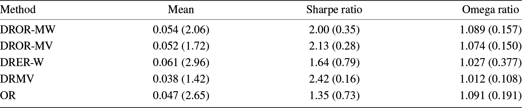
4.2. Stock market
The DRO framework has been criticized for being conservative, with a pessimistic bias in its forecasting. For instance, Hu et al. [Reference Hu, Niu, Sato and Sugiyama9] trained models that minimize adversarial reweighting and account for worst-case distribution changes. However, the model’s predictions are based on the training data performed pessimistically on the test set. To determine whether the proposed framework is overly conservative in the up-trending market and more effective in controlling losses during the down-trending market, we run the aforementioned models separately in bear and bull markets.
We focus on the stock market between 2007 and 2020. The global financial crisis, triggered by the subprime crisis in 2008, led to an overall decline in the stock market, characterized by a bear market. For our analysis, we selected data from 2007 to 2009. In the remaining period (2010 to 2020), the stock market as a whole rose and behaved as a bull market.
4.2.1. Bear market
We consider a selection of well-known stocks from various industry sectors of the US stock market for the empirical analysis, with the selected stock codes shown in Table 3, where  $\mathbf {X}=(X_1,\ldots,X_{10})^\top$ is a 10-dimensional vector, where Xi represents the ith stock return for $i = 1,\ldots, 10$.
Table 3. The assets from the US stock market.
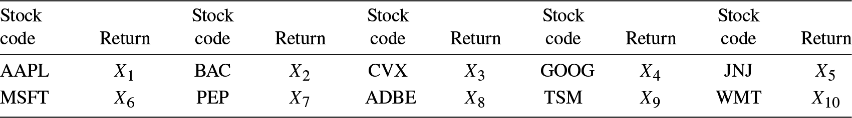
The daily returns of ten stocks were recorded as the dataset for the numerical experiment. The sample period for these historical return values is from 1 January 2007 to 31 December 2009, with 755 valid observations, that is, N = 755. Table 4 gives the means, variances and the correlation coefficients for the ten stocks.
Table 4. Means, variances and correlation coefficients of stock returns.

Due to the limited sample size, it is impossible to determine the accurate distribution of stock returns. In this paper, the ambiguous distribution of stock returns is estimated from several observations in the dataset. More specifically, the central distribution of the Wasserstein uncertainty set is a discrete empirical distribution, while the radius of the Wasserstein uncertainty set represents the imprecision of the distribution. We derive some theoretical results under the proposed mean-variance uncertainty set and the mean-Wasserstein uncertainty set in Sections 2 and 3, respectively. Theorems 3.1 and 3.5, respectively, give the investment weights for maximizing the worst-case Omega ratio under the mean-variance uncertainty set and the mean-Wasserstein uncertainty set, reducing the worst-case impact in the portfolio. Furthermore, the robust optimization problem in Theorems 3.1 and 3.5 is solved to obtain the optimal portfolio strategy.
Based on data from the US bear market, we employed a 30-day sliding time window with an initial wealth of 1. Using the data from the first 30 days, we selected the best-weighted portfolio for day 31 and calculated the returns obtained under the DROR-MV and DROR-MW models. We also considered the DRER-W and DRMV models, the non-robust OR model and the classical  $1/n$ portfolio model for comparison. The $1/n$ portfolio model, also known as the equal weighting model, is a strategy that allocates equal capital to each asset in the portfolio and is a simple yet effective approach. The results are shown in Figure 1.

Figure 1. Cumulative returns of optimal portfolio strategies under different models over the period 2007 to 2009.
Figure 1 shows the cumulative portfolio returns under the six models. The figure demonstrates that, in terms of model robustness, the DROR-MV and DROR-MW models are more effective at controlling losses during economic decline, followed by the DRMV and  $1/n$ models, and lastly, the DRER-W and OR models. This is because the DROR-MV and DROR-MW models aim to maximize the worst-case Omega ratio, which considers both returns and losses. While the DRER-W model performed the best in cumulative returns, it does not account for losses and is less stable in volatile market. The DRMV model minimizes variance, which can result in lower overall returns for portfolios with constant returns and zero variance.
4.2.2. Bull market
We have selected the same 10 stocks with a total of 2,515 valid observations from 2010 to 2020. Table 5 gives important characteristics of the returns of the 10 stocks, including the means, variances and correlation coefficients.
Table 5. Means, variances and correlation coefficients of stock returns.

We used the data of the first 30 days for portfolio selection of the best weight for day 31 and calculated the change in returns under different models, and the results are shown in Figure 2.
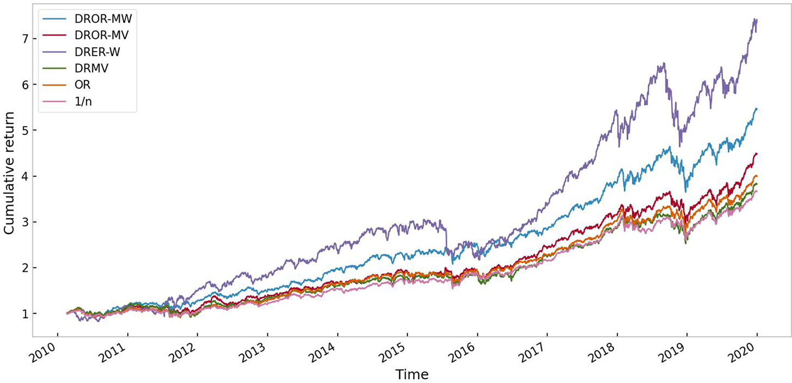
Figure 2. Cumulative returns of optimal portfolio strategies under different models over the period 2010 to 2020.
As shown in Figure 2, in terms of the final cumulative returns of the six models, the DRER-W and DROR-MW models lead by a substantial margin. The second-tier league includes the DROR-MV, OR and DRMV models. The classical equal-weighting model lags behind. This is due to the DRER-W model, which aims to maximize portfolio returns and obviously outperforms the other models. In contrast, the DROR-MV and DROR-MW models maximize the worst-case Omega ratio, while the DRMV model aims to minimize variance, which is not monotonic with respect to returns.
In summary, the DROR-MW and DROR-MV models perform well in a bear market as they consider loss and robustness, controlling losses more than classical non-robust models during large price swings. At the same time, the DROR-MV and DROR-MW models have higher returns than the classical non-robust models in a robust long-term bull market and perform less conservatively.
4.2.3. The Influence of the Wasserstein Radius ɛ
The parameter ɛ represents the radius of the Wasserstein uncertainty set, and its value determines the size of a Wasserstein ball. In other words, as ɛ increases, the Wasserstein ball becomes larger.
To obtain a relatively suitable Wasserstein radius, we refer to relevant literature to choose the value of the radius for numerical experiments. Typically, we take  $\varepsilon_0 = (\log N/N)^{1/d}$ as the radius. In the numerical experiments, we calculate the portfolio return results for the cases ɛ = 0, $\varepsilon_0/2$, $3\varepsilon_0/4$ and ɛ 0.

Figure 3. Cumulative returns of optimal portfolio strategies under different ɛ.
The calculation results show that small changes in ɛ can have a large impact on the solution of the model. Thus, the optimal solution for the investment weights is highly sensitive to the parameter ɛ. The calculation results of the portfolio strategy’s returns for different values of ɛ are presented in Figure 3. The results show that the optimal portfolio allocation varies based on the radius ɛ of the Wasserstein uncertainty set, and we obtain a relatively diversified portfolio strategy.
Acknowledgments
The authors express their gratitude to the Editor, an anonymous referee, Tiantian Mao, and Qinyu Wu for providing insightful comments on an early version of the paper. Xinqiao Xie is the corresponding author.
Competing interests
The authors declare no conflict of interest.


 Open access