


 , with B and b as parameters. This differs from the distribution of
 1. Introduction
During the period 7 to 10 April 1976 the nuclear submarine U.S.S. Gurnard (SSN–662) obtained a sonar profile of length 1 400 km under the Beaufort Sea ice cover in the vicinity of the AIDJEX (Arctic Ice Dynamics Joint Experiment) main camp. Figure 1 shows the route followed by Gurnard, comprising south-north (opq) and east-west (rsp) legs intersecting near the Caribou camp (c), together with a connecting leg qr. Gurnard was equipped with a high-frequency, narrow-beam, upward-looking sonar installed by the Arctic Submarine Laboratory, Naval Undersea Center, San Diego. The sonar fed its output into a signal-processing system that digitized the range to the bottom of the ice, subtracted this from the transducer depth, and thus generated a digital record on magnetic tape of ice drafts with a nominal resolution of 0.03 m. Mechanical limitations within the system reduced the absolute accuracy of ice draft to ±0.3 m, with a demonstrated standard deviation for smooth ice of 0.09 m. Details of the sonar system and of the submarine’s depth and speed remain classified, except that (Figure 1) information was supplied on the “surface beam diameter” (diameter of spread of the sonar beam at the surface, a function of beam width and cruising depth) and the “ping spacing” (horizontal distance between successive sound pulses, a function of ping frequency and submarine speed). Normally the ping spacing was between 1.3 and 1.5 m, and the surface beam diameter over almost the whole track was 3.17 m, implying a very narrow beam of less than 3° width.
Route of U.S.S. Gurnard, 7–10 April 1976.

Initial processing of the tapes was done at the Arctic Submarine Laboratory. Corrected depth data were merged with positional information to give a final tape which was forwarded to the AIDJEX Project Office in Seattle for analysis. In turn the AIDJEX Project Office forwarded the tape to the Scott Polar Research Institute so that the data could be analysed using the same criteria and definitions as those employed in the analysis of data from H.M.S. Sovereign (Reference WadhamsWadhams, 1977, Reference Wadhams and Pritchard[c1980], Reference Wadhamsin press; Reference Wadhams and LowryWadhams and Lowry, [1977]). This paper gives the results of such an analysis.
2. Data Processing
The initial processing at the Arctic Submarine Laboratory deleted spurious profile points caused by multiple echoes, fish, air bubbles, etc. For isolated spurious points, a new point was generated by linear interpolation; otherwise a gap was left. The data file created at San Diego consisted of a series of “blocks” each containing about 60 data points. The blocks were separated by single lines which usually contained all zeros, but which at periodic intervals contained a position fix (i.e. latitude and longitude values). These position fixes thus split the data file into “intervals” for which the distance travelled is known.
The program developed at Scott Polar Research Institute split the input file into “sections”. Each section contained sufficient intervals to make up 50 km of data, and statistics were computed for each of the sections. Figure 2 shows the 27 sections involved (with an 18 km end-of–file gap between sections 12 and 13) and their precise positions and lengths are given in Table I.
Positions of the 50 km Sections

Division of track into 50 km sections.

The actual depth data from the Arctic Submarine Laboratory came in the form of equallyspaced depth points, the spacing being unspecified and varying from interval to interval. For every interval the SPRI program therefore had to calculate an “interpolation length”, the true spacing between depth points, by dividing the length of the interval (calculated assuming a Great Circle track between the position fixes for the beginning and end of the interval) by the number of points in the interval. The contribution made by each interval to the overall statistics for a 50 km section was then always weighted by the interpolation length, so that the resulting statistics are unbiased with respect to horizontal length.
Figure 3 shows a small part of the profile. The two most obvious features are a highfrequency noise superimposed on the supposedly smooth ice bottom contour, and the occasional shallow depth point occurring within the structure of a pressure ridge. The noise is undoubtedly a feature of the recording system and, since it is random, it does not have a serious effect on probability densities of draft, although it will produce an anomalously high number of very small “pressure ridges” in the statistics. The shallow depth points are probably real features, caused by the very narrow sonar beam probing into fissures and crannies within the loose block structure of the ridge. The effect of these points may be quite large in causing a single pressure ridge to appear as multiple ridges in the statistics.
Plot of 800 m of ice-depth data from section 1.

3. Probability Density of Ice Draft
3.1. Definition
The probability density function P(h) of draft h is defined such that P(h) dh is the probability that a random point on the ice underside has a draft between h and (h+dh). P(h) should really be expressed in the form P(h, x, t) since it is a function of time as well as of position. Further, although P can be stochastically defined at a point x, an operational definition (Figure 4) requires a profile to be taken over a finite length scale in order to arrive at a stable estimate of P. This length scale must be large enough to give a good estimator of P while being small enough for the distribution not to change significantly within its compass. We have chosen 50 km, but some analyses have been done over shorter (17 km) and longer (200 km) length scales, where necessary.
Probability-density function of ice draft for 50 km sections. Depth increment 10 cm. (a) and (b), (c) and (d), (e) and (f) are pairs of perspective views for the sections that make up each of the three legs of the cruise.

P(h) is related via the mean density of the ice to the thickness probability density function g(h) of Reference Thorndike, Thorndike, Rothrock, Maykut and ColonyThorndike and others (1975). g(h) is important as an input parameter to various models of Arctic Ocean ice dynamics and thermodynamics. These include the AIDJEX model (Reference Coon, Coon, Maykut, Pritchard, Rothrock and ThorndikeCoon and others, 1974), in which an initial ice-thickness distribution develops by thermodynamic growth and decay and is continuously redistributed by pressure-ridge building and deformation, and the viscous-plastic continuum model of Reference HiblerHibler (1979), in which a strength term is parameterized using the mean ice thickness and percentage ice cover. The most sensitive part of P(h) is the thin ice component, since it has been shown (Reference Badgley and FletcherBadgley, 1966; Reference MaykutMaykut, 1976) that a large portion of the heat flow from ocean to atmosphere in the Arctic occurs through ice of draft less than 1 m; this is also the ice component which is most readily available for ridge building and which dominates the ice strength in most ice models.
3.2. Results
Figure 4 shows P(h) plotted for all 27 sections of the 50 km length scale, in a perspective form with each of the three legs shown separately. Figure 5 is an overall distribution for the whole submarine track. The general nature of ail the plots is similar—an initial peak, due to thin ice in leads and polynyas, a second broader peak due mainly to undeformed first- and multi-year ice, and a tail due to ice in ridges and hummocks. There is some variation from section to section, especially in the extent of thin ice present.
Overall probability-density function of ice draft.

To display these variations more clearly, P(h) was integrated over four depth intervals, which can be loosely defined as “thin ice” (0–0.5 m); “young ice” (0.5–2 m); “level ice” (2–5 m), and “ridged ice” (greater than 5 m). The separation of types is not perfect—parts of ridges, for instance, may appear in the “level ice” category—but the categories are indicative of changes in the nature of the ice cover. The results are given in Table II. The intervals were chosen so as to give a direct comparison with the data of Reference Wadhams and PritchardWadhams ([c1980], in press) from the heavily ridged offshore zone to the north of Greenland and Ellesmere Island. Wadhams found that the “thin-ice peak” in probability-density functions usually occurred at less than 0.5 m draft, hence the choice of intervals, but the present results (Fig. 4) usually show the peak at (Figure 5) (Table II) between 0.5 and 1 m, presumably because the profiles were done later in the winter (April compared to October for Sovereign) so that the ice in polynyas is, on average, thicker. Thus we have also added a 0–1 m category in Table II to include all of the polynya ice.
Percentages of Ice Cover in Different Ranges of Draft

The results show a remarkable consistency of ice conditions over most of the experimental area. The exceptions are:
-
(i) The percentage of thin ice, which varies over a wide range (0.4 to 12.3% for the 0–1 m band) and with no apparent consistency of trend. The cause is partly statistical —thin ice is contained in a limited number of polynyas which are distributed non-uniformly along the submarine track—and partly real in the sense that thin ice has a transient existence and is constantly being destroyed by ridge-building so that changes in the wind field during the three days of the experiment may cause the thin ice to be radically redistributed.
-
(ii) Ridged ice at the southernmost (and, to a lesser extent, the westernmost) end of the profile is significantly greater in quantity. The percentage of ridged ice is very high in section 1 and diminishes to a fairly steady “equilibrium value” by section 3. Clearly the first two sections represent the “offshore province” of Reference Weeks, Weeks, Kovacs, Hibler, Wetteland and BruunWeeks and others ([1972]), a heavily ridged coastal province where the mean onshore tendency of ice drift leads to net convergence and ridge building. To a lesser extent sections 26–27 mark the outer edges of this province further to the west. These results agree very well with surface ridging statistics from flights northwards from the Alaskan coast (Reference Tucker, Tucker, Weeks and FrankTucker and others, 1979), which revealed a maximum of ridging at 20–60 km from the coast, falling to a low value at 200 km (equivalent to the end of section 3). Figure 1 shows that sections 1 and 2 occur over the continental slope (the profile itself commences at the 100 m depth contour) and that section 27 ends just as this slope is again approached off Point Barrow. The remainder of the sections are samples of what seems a very homogeneous ice cover.
The mean values over all 27 sections are compared in Table II with the mean results from Sovereign (1 000 km profile from lat. 81° N., long. 0° W. to lat. 84° 50' N., long 70° W.) and Dreadnought (a 560 km profile from lat. 85° to 90° N. at long. 6° E. in the ice of the Trans-Polar Drift Stream; Reference Williams, Williams, Swithinbank and RobinWilliams and others, 1975). The best agreement is with the Dreadnought data, although the Gurnard data show a somewhat lower mean draft which can be ascribed to the beamwidth of the Dreadnought’s echo sounder. Clearly the ice encountered by Sovereign was far more heavily ridged and thicker than even the heaviest section encountered by Gurnard.
The 50 km gauge is short enough to resolve most real variations, but to investigate the rapidly changing ice conditions at the beginning of the profile (sections 1 and 2) a 17 km gauge was used, i.e. each section was split into three. The results, in Table II (b), show a steady decrease in the percentage of ridged ice as the submarine travels north away from the Alaskan coast. Note the isolated value of 13.3% for 0–1 m ice in section 1.2.
Finally, to obtain very reliable statistics for large tracts of the ice cover, the 50 km sections were combined into a 200 km length gauge as shown in Figure 2, lettered a to g (a is 150 km only), b and f are now the appropriate sections for the crossings under Caribou camp, and have the length scale recommended in the AIDJEX model and by Reference Thorndike, Thorndike, Rothrock, Maykut and ColonyThorndike and others (1975). The results for b and f agree very closely. Again, the 200 km statistics show that the character of the ice is essentially constant over most of the track (b to f), with an increase in mean draft and percentage of ridged ice at the western end (g) and, particularly, the southern end (a).
3.3. Statistical reliability
It is clear from Table II(b) that there are progressive changes in the nature of the ice cover over sections 1 and 2, and that these sections (and probably 26 and 27) differ in nature from sections 3–25. The question that remains is whether the variations between sections in 3–25 are statistical artefacts, i.e. due to finite sampling length, or whether they are due to real variations, albeit minor, in the nature of the ice cover. The null hypothesis is that the ice cover over a substantial part of the southern Beaufort Sea (the area sampled by sections 3–25) at the time of the experiment was a homogeneous cover in which any given statistical parameter tends to the same value everywhere if sampled over a sufficient length of track.
The question of “sufficient length” is a crucial one. For a given sampling length, some parameters are estimated more accurately than others. For instance, 50 km of track usually contains enough ice types to make it a good estimator of mean draft, and most probably of percentage ridged ice. It may not be a good estimator, however, of thin ice percentage since this ice is contained in a small number of polynyas which may not happen to fall uniformly within the length gauge. A longer gauge may be required for a good estimate of this parameter, and also of such parameters as mean polynya spacing or the frequency of very deep pressure ridges.
we can test for the homogeneity of the data using a non-parametric run test (Reference Bendat and PiersolBendat and Piersol, 1971, p. 122). The data are divided into n sections for which a given statistic S takes values S j (j = 1,..., n). The mean value of S is calculated and each section is classified as (+) or (—) according to whether

Test for Homogeneity of Data

Only one statistic—the 0–0.5 m percentage cover for the 50 km sections—was rejected by this test at the 25% significance level. This implies that the thin ice percentage does not come from a homogeneous population, i.e. that there are significant trends or clusterings in this statistic (which can be seen by inspection of Table II) suggestive of a process acting with a wavelength much greater than 50 km. This process must be the wind stress field which causes divergence in one zone of the ice cover and convergence in another, on a length scale of hundreds of kilometres.
Otherwise we can accept the hypothesis that the ice draft distributions over 1150 km of track in the southern Beaufort Sea (3–25) come from a homogeneous ice cover with constant statistical properties. The best values to take for the mean draft and percentages of ice in various depth ranges are given in Table III, together with the standard error. It can be seen that this standard error is virtually constant for each class (except 0–0.5 m), implying a greater fractional error in the estimates of uncommon ice types than in those of common types—a result to be expected.
3.4. Cumulative probability
The cumulative probability G(h) is defined by

It is used as a major parameter in the AIDJEX model (Reference Coon, Coon, Maykut, Pritchard, Rothrock and ThorndikeCoon and others, 1974). We have computed G(h) for the two 200 km sections b and f which cross the Caribou camp in the south-north and east-west directions. The results are shown in Figure 6.
Cumulative probability distribution G(h) of ice draft for the two 200 km sections which straddle the Caribou camp.

The two distributions differ slightly but are similar in general shape. The median depth (G(h) = 0.5) is reached at 3.2 m and the graph is plotted as far as G(h) = 0.99, which is reached at 12.2 m, G(h) = 0.999 is reached at 16.4 m.
4. Level Ice
4.1. Definition
Reference Williams, Williams, Swithinbank and RobinWilliams and others (1975), in their analysis of the Dreadnought data, sought a way of determining the preferred thickness or thicknesses of undeformed floes, and the percentage of the ice cover occupied by floes of this type. By trial and error they decided that the best working definition of “level ice” is that the draft point concerned should have draft points 4 m to each side of it differing in depth by less than 20 cm, i.e. a local gradient of less than 1 in 40 measured on an 8 m gauge length across the point. On account of the high-frequency structure in the Gurnard profile (Fig. 3), we have relaxed this definition slightly and we define a level ice point as one whose draft differs from a point 10 m away to either side by less than 25 cm, i.e. a 1 in 40 gradient in one direction moving away from the point. This definition has the disadvantage that it includes ice on opposite flanks of a pressure ridge at a depth where the ridge width is 10 m, and ice on the same flank of successive ridges where the ridge separation is 10 m. However, any working definition must be to some extent arbitrary and this definition when applied to the Dreadnought profile gave results which corresponded well with visual estimates of percentage of level ice made by simply looking at the profiles and dividing them by eye into “level” and “ridged” portions. We assume, therefore, that the contribution from ridge flanks is small enough to make only a minor contribution to the amount of “level ice” found, although it may well make a larger contribution to the mean draft of “level ice”, a figure which we should treat with reserve.
Alternative definitions of level ice have been suggested by A. S. Thorndike (personal communication in 1978). One proposed definition (D2, say, taking our definition as D1) is that no point within 10 m of a level ice point may differ in draft by more than 25 cm from that of the level ice point. Thus, taking [x, h(x)] as the level ice point:

D2 is much more restrictive than D1. Figure 3 shows that the Gurnard profile possesses a large high-frequency variance which may be a recording artefact, and in such a profile D2 finds far less level ice than D1 (an average of only 20% instead of 56%). We feel that D2 does not reveal the true extent of level, i.e. undeformed, ice, and that D1 represents this more nearly. On the other hand D2, being so rigorously selective, is effective at picking out the preferred drafts of level ice (i.e. it is not seeing all the level ice, but all that it sees is level ice). Thus, for seeking preferred drafts D2 may be the better definition.
4.2. Results
Figure 7 shows probability density functions of level-ice draft for all 27 sections at 50 km gauge, using D2 to emphasize the preferred drafts and the same perspective form as Figure 4. In Figure 8 these results are summed to give relative probabilities over the whole track length. In Table IV we show results obtained from using D1; preferred drafts are indicated here by listing the mode of every distribution if its probability density is greater than 0.5 plus the thin ice peak if it exceeds 0.1
Probability-density function of level-ice draft for 50 km sections, derived using definition D2. The pairs of perspective views cover the three legs of the cruise.

Overall probability-density function of level-ice draft.

Level Ice Summary

The figures given in Table IV for percentage ice cover are probably reliable although undoubtedly slight over-estimates; the figures obtained using D2, ranging from 8 to 24%, are unrealistically low. The mean draft in Table IV may be more of an over-estimate and here we may consider the D2 values (with an overall mean of 2.66 m) as being more representative. The percentage of level ice is low for sections 1 and 2 with their heavy ridging; steady for sections 3 to 25 (passing a run test for homogeneity) ; and lower again in sections 26 and 27.
Figures 7 and 8 and Table III all tell us something about preferred drafts. It is clear from Figure 7 that for individual 50 km sections the probability distribution is not smooth, but instead possesses a definite small number of peaks indicating strongly preferred drafts; there are usually one or more thin-ice peaks and two definite peaks in the range 2–3 m. The obvious inference is that the first peak in the 2–3 m range represents first-year ice and that the second, ((Figure 8) Table IV) which is often somewhat broader, represents second- and multi-year ice. Figure 8, the overall distribution, also shows these peaks. Here there are two thin-ice peaks, at 0.3–0.4 m and 0.8–0.9 m; and two main peaks, at 2.1–2.2 m and 2.7–2.8 m. Table IV bears out these results; the main peak is most often at 2.7–2.8 m, with 2.0–2.1 m and 3.1–3.2 m as less frequent peaks, the 3.1 m figure occurring mainly in the south and west of the experimental area where there is heavier ridging.
Can we say, then, that 2.0–2.2 m, 2.7–2.8 m, and 3.1–3.2 m represent, say, the drafts reached by first-, second-, and multi-year undeformed ice? According to present thermodynamic theories of ice growth in Arctic Ocean, we cannot. The estimates of Reference Thorndike, Thorndike, Rothrock, Maykut and ColonyThorndike and others (1975), based partly on the theory of Reference Maykut and UntersteinerMaykut and Untersteiner (1971) and partly on empirical results and observations of thin ice, show that ice growing from open water at the end of summer will reach a thickness of 1.76 m by 10 April of the following year, and 2.04, 2.21, and 2.35 m by 10 April of its second, third, and fourth years of growth. All these values, and the yearly depth increments between them, are less than the preferred level-ice drafts that we have found. The identification of level-ice draft with ice type therefore remains an open question, although these results do suggest that undeformed ice grows to a greater thickness than that estimated by thermodynamic theories.
The thin-ice end of the probability distribution (Fig. 8) indicates the relative frequencies of occurrence of polynyas of varying ages.
5. Distribution of Keel Spacings
5.1. Independent keels
The extent of an independent keel is defined using the criterion that the troughs on either side of the keel crest (point of maximum draft) must descend at least half way towards the local level ice surface, in this case defined arbitrarily as a draft of 2.5 m. This is analogous to the Rayleigh criterion for resolving spectral lines in optics and is identical to that used by Reference Williams, Williams, Swithinbank and RobinWilliams and others (1975), Reference WadhamsWadhams (1976, Reference Wadhams and Pritchard[c1980], in press), and Reference Weeks, Weeks, Tucker, Frank, Fungcharoen and PritchardWeeks and others ([c1980]) for the analysis of submarine and aircraft profiles (for airborne laser profiles the identification of the “local level ice surface” is much easier). It differs from the criterion of Reference Hibler, Hibler, Mock and TuckerHibler and others (1974), where the troughs must descend a fixed distance (61 cm for surface ridges) from the peak; Reference HiblerHibler ([c1976]) has discussed the effect of this difference in definition on the resulting distribution.
5.2. Theory of spacings
Reference Hibler, Hibler, Weeks and MockHibler and others (1972) showed that if ridges occur at random along a track the distribution of spacings between ridges is given by

where μ is the mean number of ridges per unit length of track and P r(x) dx is the probability that a given spacing lies between x and (x+dx). Reference Mock, Mock, Hartwell and HiblerMock and others (1972) tested this relationship for surface ridges using aerial photographs, and found good agreement except for an excess of ridges at small spacings. On a purely random theory, however, we expect a deficit of ridges or keels at small spacings, on account of the so-called “ridge shadowing” effect (Reference Wadhams and PritchardWadhams, [c1980], Reference Wadhamsin press). This occurs because keels have a finite slope angle so that their crests cannot lie closer than a certain minimum distance x crit. Within this distance the shallower ridge is not detected and the ridge-picking criterion selects only the deeper ridge. Figure 9 illustrates this effect for two keels of relief h, h’ (h’ > h) relative to the level-ice bottom, each ridge being of triangular cross-section with slope α. Under these circumstances

A theoretical treatment of the modification of Equation (2) by Equation (3) is complex, but an approximate solution is given by Reference Lowry and WadharmsLowry and Wadhams (1979). The net effect is that close spacings and shallow ridges tend to be lost preferentially from the distributions of spacing and draft.
Illustration of the keel shadowing effect for two keels of separation x and relief h, h′ relative to local level ice draft.

5.3. Results
Keel spacing distributions were derived using a spacing increment of 20 m and two low-value cut-offs for keel draft, 5 m and 9 m. This is because Reference Wadhams and PritchardWadhams ([c1980], in press) found that a number of deep floe bottoms appeared in the draft range 5–9 m and that the theoretical keel draft distribution function was valid only beyond 9 m. It was felt, therefore, that by taking 9 m as a cut-off a more valid distribution of spacings of “real” keels could be obtained. The results for the whole profile are shown in Figure 10.
Distribution of keel spacings over whole submarine track. Bin size 20 m. Results are plotted for keels deeper than 5 m and 9 m, and a straight line is fitted to the central portion if each curve.

Both distributions (>5 m and >9 m) show general agreement with Equation (2), with the expected deficit at small spacings. This deficit shows itself only in the spacing range 0–40 m, as opposed to the results of Wadhams (1979, fig. 4), where the deficit extends its influence to 120 m. This is probably because of the transducer beam width in the Sovereign profile, which makes ridges seem broader and less steep than they really are (Reference Wadhams and MuggeridgeWadhams, 1978). At large spacings Figure 10 shows a positive deviation from Equation (2), which must be due to an additional effect upsetting the purely random distribution. We suggest that this effect is simply the presence of leads and polynyas, which interpose occasional smooth stretches of ice into the otherwise random icefield and thus generate an anomalous number of large keel spacings.
It should be noted that the lines of best fit to the rectilinear parts of Figure 10 do not have a gradient of −μ For the 5 m cut-off the gradient is −5.2 (μ = 7.3) while for 9 m it is −2.9 (μ = 1.7). One expects a gradient of magnitude than μ because keel shadowing implies that the original “population” has been reduced before entering the statistics. This is (Figure 9 and Figure 10) so for 9 m but not for 5m, again implying that 9 m is a better cut-off to use to obtain a population of “pure” keels.
We also present a tabulation of spacings classified according to the depth of the deeper keel of the pair which defines the spacing, i.e. a tabulation of x against (h’+2.5 m) in Figure 9. This is an attempt to find the best α for use in Equation (3). The results for 9 m cut-off are plotted in bins of 2 m depth increment and 20 m spacing increment. The curves (Fig. 11) show a peak at a spacing which progressively increases with depth. In Figure 11 the position of the highest peak in each curve has been plotted against the relevant depth (the heavy black dots), and it can be seen that the increase with depth is roughly linear. A line of best fit has been drawn through these points which, when applied to Equation (3), gives a value of 13.3° for α. Of course, these curves show that there is no one value of α, otherwise there would be a sharp spacing cut-off within which no keel pairs are to be found. Instead, there is a range of α, a range which is spread out still further by the fact that the keels are not being profiled orthogonally but at various angles of encounter. Reference Wadhams and MuggeridgeWadhams (1978) dealt with this statistical averaging problem. Our value of 13.3° is, in any case, an underestimate because it refers to the peak of each spacing distribution rather than to the spacing at which keel pairs begin to be found. However, it is indicative of the validity of the “keel shadowing” concept. Again, by actually measuring the slopes of keels on sonar profiles, Reference Wadhams and MuggeridgeWadhams (1978) found that the slope-angle distribution had a peak in the range 16–20° but, when adjusted to take account of the angle of encounter, the mean value of α came to 32°. Thus our 13.3° figure does not appear unreasonably low.
Spacing distributions for keels of draft greater than 9 m, in 2 m draft increments. The spacing corresponding to the maximum of each distribution has been plotted as a heavy black dot. This spacing increases linearly with keel relief.

6. Distribution of Keel Drafts
6.1. Theory
The theory of keel drafts which has been most extensively tested against observation is that of Reference Hibler, Hibler, Weeks and MockHibler and others (1972). They used a variational calculation which gives the most likely distribution of geometrically congruent ridges that will yield a given volume of deformed ice. The result is

where P r(h) dh is the probability that the draft lies between h and (h+dh), h is the mean draft, h 0 is a low-value cut-off below which keels are not included in the statistics, and λ is a parameter which must be derived by iteration from

This has been shown to give a better fit to submarine sonar observations than an alternative distribution proposed on empirical grounds by Reference DiachokDiachok (1975):

with

Recently it has been found that surface ridge sails, to which this theory was also thought to apply, actually obey a simpler negative exponential distribution of form

with B and b as parameters, provided the sails are identified using the Rayleigh criterion (Reference WadhamsWadhams, 1976; Reference Weeks, Weeks, Tucker, Frank, Fungcharoen and PritchardWeeks and others, [c1980]). Reference HiblerHibler ([c1976]) showed that the same data can be made to fit Equation (4) or Equation (7) depending on whether the Hibler (constant trough depth) or Rayleigh ridge-picking criterion is used.
6.2. Results
Figure 12 shows the distribution of keel drafts for various length gauges, expressed as keels per 100 km track and using a 1 m depth increment. “Keels” of less than 5 m draft can be assumed to consist mainly of the bottoms of undulating floes, and so have not been plotted.
The result is a good fit to a straight line on a semilogarithmic plot, not only for the overall data but also for data at 400 km gauge (sections F and B, shown in Fig. 12) and even 50 km gauge (section 1, Fig, 12). This shows that the keel draft distribution obeys the simpler relationship of Equation (7) rather than the Hibler relationship, Equation (4). This is a most unexpected result, because Equation (7) was hitherto thought to be valid only for ridge sails; the Sovereign keel data, analysed using the Rayleigh criterion, follow Equation (4) with a high degree of exactness as do all other published sonar profiles. Reference Wadhams and PritchardWadhams ([c1980], Reference Wadhamsin press) suggested that sails may not follow Equation (4) because they contain only a small proportion of the mass of a ridge and their shape is determined largely by accident. This cannot explain the present result. We must conclude either that keels in the Beaufort Sea have a different nature from those in the Eurasian Basin, which is unlikely, or that the apparent distribution of independent keel drafts is dependent in some way on the type of sensor employed.
Distribution of keel drafts plotted on a semilog plot for data at 1 400 km, 400 km, and 50 km length gauges.

Profiles of ridge sails are typically obtained using a laser profilometer; which has a pencil beam capable of recording much of the fine structure of the sail, including crevices and troughs between the blocks (the limitation being the integration time of the laser electronics). The sonar employed by Gurnard also had a narrow beam-width and, as shown in Figure 3, it also appears capable of recording the fine structure of a keel, probing into clefts and hollows between the submerged blocks. Dreadnought (Reference Williams, Williams, Swithinbank and RobinWilliams and others, 1975) used a sounder with a very wide beam, and Sovereign (Reference WadhamsWadhams, 1977) had a sounder with a wide beam in the fore-and-aft plane (17°) and a narrow beam in the athwartships plane (5°). Wide-beam sounders smooth out the structure of a keel so that it is always perceived as a single wedge (see, for example, the profiles in Reference Wadhams and MuggeridgeWadhams, 1978), and even the application of reconstruction equations (Reference Williams, Williams, Swithinbank and RobinWilliams and others, 1975) cannot regenerate this fine structure. Now Hibler’s theory depends on the concept of geometrically congruent ridges, each an entity of the same shape possessing mass and potential energy which depend only on its depth. A wide-beam sounder forces keels to approximate to this concept by smoothing out any incidental structure that they may possess and leaving them as discrete entities. Thus narrow-beam echo sounders and laser profilometers produce one type of ice profile with ridge height characteristics obeying Equation (7), while wide-beam sounders produce another type, obeying Equation (4). A narrow-beam sounder, by splitting many ridges into multiple “ridges”, sees a greater ridge frequency than a wide-beam sounder (e.g. in Reference Wadhams and PritchardWadhams ([c1980], Reference Wadhamsin press) the sail frequency is a multiple of the keel frequency for the same ice cover).
This hypothesis now covers all results except the laser profilometer data reported by Reference Hibler, Hibler, Mock and TuckerHibler and others (1974), which still obeyed Equation (4) but which were not analysed on the Rayleigh criterion. A crucial test of the hypothesis would be to smooth the Gurnard profile artificially by convolving it with the beam pattern of a wide-beam echo sounder, and to observe the effect on the resulting statistics. We hope to report on this computer simulation in a later publication.
It was shown in Reference Wadhams and PritchardWadhams ([c1980], Reference Wadhamsin press) that the parameters B and b in Equation (7) can be expressed as simple functions of h and μ. If Equation (7) is rewritten in the form

where n(h) is the number of keels per kilometre of track per metre of draft increment, then

and

so that

and

Pressure-ridge Frequencies and Mean Drafts for 50 km Sections

Thus μ and h are the two parameters of the keel draft distribution from which the whole shape of the distribution can be deduced using Equations (8) to (12). Table V shows these parameters tabulated for all the 50 km sections, using h 0 = 5 m and 9 m so as to be consistent with the statistics of Reference Wadhams and PritchardWadhams ([c1980], Reference Wadhamsin press). The results are also plotted in Figure 13. The following conclusions can be drawn:
-
(a) he major part of the profile (sections 3–25) has a ridging distribution which is very homogeneous and which falls within narrow limits of variation. These limits are extremely narrow for h 0 = 5 m (5.4–8.2 for μ; 7.2–7.8 m for
) and somewhat wider for h 0 = 9 m. probably because of the smaller number of keels involved. Means and standard deviations for these four parameters are given; run tests show that we can accept the hypothesis of a homogeneous ice cover with respect to ridging intensity.
-
(b) Sections 1–2 and 26–27 fall clearly outside the range of variation of the other sections Figure 13, indicating much heavier ridging (greater μ) in these parts of the track. This result agrees with what we have found from the probability-density functions; at these two extremities of the track there are more pressure ridges per unit length, a greater mean keel draft, a greater mean ice draft, and a greater proportion of deformed ice. Reference Tucker, Tucker, Weeks and FrankTucker and others (1979) measured surface-ridge (>0.9 m high) frequencies from a laser flight northward from Barter Island in April 1976, and found a peak of about 13 ridges per km at 80 km from the coast, falling to 2.5 per km at 200 km from the coast. These parts correspond to sections 1 and 3 respectively, and Figure 13 shows that there is fair agreement between these results and the frequencies of keels greater than 5 m deep.
-
(c) There is no clear positive correlation between μ and h , although the four heavily ridged sections have both a high μ and a high h .
-
(d) For h 0 = 9 m both the frequency and the mean draft are much lower than those found by Sovereign in the very heavily ridged zone off north Greenland. Only section 1 exceeds the Sovereign data in keel frequency, though not in mean draft. The data compare very well with Dreadnought data from the central Eurasian Basin: although it may appear from Table V that Dreadnought data have a lower μ h , the difference can be ascribed to the program of Reference Williams, Williams, Swithinbank and RobinWilliams and others (1975) which, by applying a harsh version of the Rayleigh criterion with sea-level as the zero datum, lost many shallow keels from the statistics.
-
(e) The maximum drafts are surprisingly low. On the whole the deepest keel drafts are found in the four anomalous sections (1–2, 26–27), but the deepest draft of all, 31.12 m, in fact occurred in the short 18 km portion of track that was omitted from the 50 km statistics. The general ridging properties of this portion (Table V) are quite typical of the sections surrounding it, so that the keel can be seen as an isolated event. This is the only keel deeper than 30 m in the entire 1400 km of profile, whereas in the Sovereign profile there were 45 keels deeper than 30 m in 3900 km of track, 39 of them occurring in the 1050 km of “offshore zone” north of Greenland (Reference Wadhams and MuggeridgeWadhams, 1978). By a coincidence the deepest keel in the Sovereign profile, 43 m, also occurred as an isolated event in an otherwise lightly ridged section of ice cover.

Mean keel draft plotted against mean number of keels per kilometre for keels deeper than 5 m and 9 m. Each point represents a 50 km section.

Finally we note that the distribution of keel drafts suggests an analytical form for the deep portion of the probability density function P(h). Beyond the maximum draft which can be attained by undeformed ice, h max say, the whole of P(h) is due to contributions from ice keels. If keels all tend to the shape of isosceles triangles with a mean slope angle α. along track (as in Fig. 9), then we have

Figure 14 shows that P(h) indeed fits a negative exponential for depths beyond 6 m. The fit is excellent both for the overall data and for a 50 km section, although the smaller number of points in the latter case introduces greater variance. The gradients and intercepts yield the following estimates for b and α given in Table VI.
Semilog plots of probability density functions of ice draft, showing fit to a negative exponential at depths beyond 6 m.

Pparameters in the Distribution Function for Keel Drafts

In each case α is calculated from Equation (13) and the intercept of Figure 14 using B found from Equation (12). The good agreement between b as found from Figure 14 and as calculated from Equation (11) confirms Equation (13) as a valid equation for the ice draft distribution at depths beyond 6 m. This simple result should be of great value to modelling studies, making it easy to calculate the ice draft distribution from a knowledge of the distribution of pressure ridges in the ice field. The best value to use for α is probably that computed from the whole track at h 0 = 9 m (since this eliminates all the deep parts of undeformed floes), i.e. 11.3°. It is noteworthy that this lies close to the value of 13.3° calculated in a quite different way from Figure 11.
7. Leads and Polynyas
The probability-density function of ice draft gives the best measure of the occurrence and thickness distribution of the thin ice in leads and polynyas, and is especially useful for application to heat-budget calculations. However, it is important for a variety of problems in ice mechanics to know the frequency and width distribution of leads encountered by the submarine. Perhaps the most important application is to submarine operations themselves—it is desirable to know the mean spacing of leads that are large enough to permit a submarine to surface.
A lead was defined as a continuous sequence of depth points in which no point excedds 1 m in draft—thus a polynya broken up by a small floe of broken ice counts as two leads. Lead width were classified in 50 increments and the results calculated for each of the three files making up the overall track (File 1 = sections 1–12; File 2 = 13–21; File 3 = 22–27). The results are shown in Table VII.
(A) Distribution of lead widths: Number of leads encountered per 100 km of track
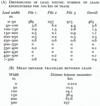
On average a lead is encountered about every 200 m, although this figure varies by a factor of nearly four between File 2 and File 3. However, the lead concerned is likely to be very narrow, and few leads exceeded 50 m in width.
Table VII(B) shows that a submarine which requires a 200 m lead for a safe surfacing will have to travel 68 km to find one. In fact a submarine trying to surface usually investigates every lead wider than about 50 m in case the cross-track dimension is sufficient to permit surfacing; 50 m leads occurred every 10 km in the southern Beaufort Sea during the period of this experiment.
Acknowledgements
The authors acknowledge with thanks the support of the Office of Naval Research under contract N00014-78-G-0003. The data transfer was arranged through the good offices of Robert S. Pritchard and Professor Norbert Untersteiner. Our thanks are also due to Murray J. Stateman, AIDJEX data manager, and to the staff of the Arctic Submarine Laboratory, San Diego, for furnishing and pre-processing of data.



