


1. Introduction
It is known that a perfectly cylindrical liquid jet or thread with surface tension acting on its interface is unstable to long wave axisymmetric perturbations; such capillary instabilities emerge for both viscous and inviscid liquid jets/threads. Rayleigh was the first to examine the linear stability of liquid jets for both inviscid (Rayleigh Reference Rayleigh1878) and viscous (Rayleigh Reference Rayleigh1892) liquids. The instability is long wave and all axisymmetric perturbations longer than the undisturbed thread circumference become unstable. The axisymmetric modes are the most unstable in the absence of other effects such as rotation about the axis (Ponstein Reference Ponstein1959), and external electric and magnetic fields (Huebner & Chu Reference Huebner and Chu1971; Saville Reference Saville1971; Eggers & Villermaux Reference Eggers and Villermaux2008) among others. Following Rayleigh's seminal works, Tomotika (Reference Tomotika1935) included the effects of a surrounding viscous fluid and found that the instability characteristics are analogous even though growth rates can be reduced by the presence of an outer viscous fluid. This problem is also discussed in the textbook by Chandrasekhar (Reference Chandrasekhar2013). For recent reviews on capillary instabilities and consequent breakup see Eggers (Reference Eggers1997) and Eggers & Villermaux (Reference Eggers and Villermaux2008).
Of interest in this article is the effect of surfactants on the linear stability of liquid threads or jets. Surfactants are molecules that preferentially adsorb to liquid interfaces, thus modulating the coefficient of surface tension. Generally, they are categorized as insoluble and soluble. Insoluble surfactants are trapped at an interface, whereas soluble ones kinetically exchange between the bulk and the interface. At low surfactant solubility, experimental observations suggest that soluble surfactants behave almost like insoluble ones, and less like monomer surfactants as solubility increases. Numerous authors have focused on the effect of insoluble surfactants on the stability of liquid threads or jets, including Whitaker (Reference Whitaker1976), Hansen, Peters & Meijer (Reference Hansen, Peters and Meijer1999), Kwak & Pozrikidis (Reference Kwak and Pozrikidis2001), Craster, Matar & Papageorgiou (Reference Craster, Matar and Papageorgiou2002) and Timmermans & Lister (Reference Timmermans and Lister2002). These studies showed that surfactants can have a large effect on jet stability. In particular, Craster et al. (Reference Craster, Matar and Papageorgiou2002) and Timmermans & Lister (Reference Timmermans and Lister2002) show that an increase in surfactant concentration leads to a decrease in the growth rates of unstable modes. In the nonlinear regime, the presence of surfactant concentration gradients leads to Marangoni forces that have been observed to slow down pinching in liquid threads or bridges – see Craster et al. (Reference Craster, Matar and Papageorgiou2002), Ambravaneswaran & Basaran (Reference Ambravaneswaran and Basaran1999) and Liao, Franses & Basaran (Reference Liao, Franses and Basaran2006). In another study Craster, Matar & Papageorgiou (Reference Craster, Matar and Papageorgiou2009) model and calculate the effects of soluble surfactants above the critical micelle concentration. They find that the nonlinear breakup mechanisms in such cases lead to unusually large satellite drops. They also briefly discuss the role of surfactant solubility, showing that more soluble surfactants increase growth rates compared with insoluble ones, with the most soluble surfactants displaying behaviour more akin to a clean interface. Such remobilization phenomena have also been observed in rising bubble experiments and simulations (Palaparthi, Papageorgiou & Maldarelli Reference Palaparthi, Papageorgiou and Maldarelli2006). When the surfactant concentrations are above the critical micelle concentration, phase transitions occur in the bulk and surfactant monomers coexist with micelles. The theoretical modelling is different, see for example Craster et al. (Reference Craster, Matar and Papageorgiou2009).
One type of surfactant that has not been studied as closely, especially in the context of stability of systems, is the so-called photosurfactant or ‘light-actuated’ surfactant, such as the ones in an early paper by Shin & Abbott (Reference Shin and Abbott1999). They are synthesized by embedding a light-switchable group such as an azobenzene (see Jerca, Jerca & Hoogenboom Reference Jerca, Jerca and Hoogenboom2022) in between a hydrophilic head and hydrophobic tail group. Due to this, these surfactants can stably exist in one of two isomer states, cis or trans, that display markedly different adsorption/desorption behaviour near interfaces. Usually, trans isomers are more surface active, and cis isomers are less. Azobenzene-type photosurfactants undergo photoisomerization under light illumination, switching between states at rates that vary with the wavelength and intensity of incident light. Specifically, ultraviolet (UV) illumination causes trans-to-cis conversion, and lower-energy light such as visible or blue light causes reversion back to trans. Due to this switching mechanism and the different interfacial behaviours of these molecules, equilibrium surface tension values in systems illuminated with UV light have been shown to be as much as  $20\ {\rm mN}\ {\rm m}^{-1}$ higher than those under blue (Shang, Smith & Hatton Reference Shang, Smith and Hatton2003). In the context of fluid mechanics, photosurfactants have been shown to be a promising means of causing externally controllable fluid transport via light-induced chromocapillary stress. For example, Ichimura, Oh & Nakagawa (Reference Ichimura, Oh and Nakagawa2000) used photosurfactants and a light gradient to modulate the liquid–solid tension of a droplet of water, thus driving the droplet through a wetting mechanism. In the context of surface-tension (liquid–gas) driven flows, point sources of UV light have been used by Varanakkottu et al. (Reference Varanakkottu, George, Baier, Hardt, Ewald and Biesalski2013) and Chevallier et al. (Reference Chevallier, Mamane, Stone, Tribet, Lequeux and Monteux2011) to generate radially inward flows of photosurfactant-seeded water, for which one application is the capture of interfacial particles at the light source. Recently, Zhao et al. (Reference Zhao, Seshadri, Liang, Bailey, Haggmark, Gordon, Helgeson, Read de Alaniz, Luzzatto-fegiz and Zhu2022) showed that light-actuated Marangoni flows can cause a droplet of a toluene solution entering photosurfactant-laden water to depin more quickly than it would otherwise.
Our goal then is to examine the effect of these photosurfactants on the linear stability of viscous liquid threads. In the present analysis we have ignored rheological effects. These are believed to be important in the behaviour of surfactant-laden interfaces, especially at larger interfacial concentrations. To model surface rheology the interface is treated as a two-dimensional compressible fluid, often by the classic Boussinesq–Scriven approximation (Scriven Reference Scriven1960). This approximation alters the traditional stress tensor by assigning the interface its own surfactant-dependant surface shear and dilatation viscosities. In the context of the stability of threads or jets, rheological effects generally have a dampening effect. For example Martínez-Calvo & Sevilla (Reference Martínez-Calvo and Sevilla2018) reported reduced instability growth rates when surface viscosity was increased and Wee et al. (Reference Wee, Wagoner, Kamat and Basaran2020) showed that the thinning rate of threads during breakup is reduced when rheological effects are included. Since surface rheology tends to reduce growth rates, we choose to ignore them presently in order to reduce the complexity of our model and to isolate the effects of the photosurfactants on the linear stability of liquid threads.
To do this, first, we begin by comprehensively describing the physical model. This is followed by a dimensionless analysis and discussion of the numerous relevant dimensionless parameters. From there, linear stability equations are derived using normal modes with significant discussion given to the base case, as it is shown a non-uniform (i.e. spatially varying) base case exists. The numerical framework used to solve the linear stability eigenvalue problem is then discussed. The results are presented in a way that provides a holistic understanding of the impact of surfactants on the threads, by comparing our numerical results with the analytical results of much simpler problems. This includes the clean interface limit of Tomotika (Reference Tomotika1935) and the insoluble surfactant work of Timmermans & Lister (Reference Timmermans and Lister2002), as well as two analytical solutions derived here for soluble surfactants and photosurfactants in a special limit. We show that photosurfactants give the ability to change the rate of growth of instabilities simply by varying the wavelengths and intensity of light but, at least under constant illumination, they have little impact on the critical wavelength below which all modes are unstable.
2. Problem formulation
We consider an axisymmetric liquid thread of infinite length that is supported by a surrounding dynamically passive fluid, e.g. air. The undisturbed perfectly cylindrical thread has constant radius  $R^*$, and under axisymmetric perturbations we denote the radial thickness by $r^*=S^*(z^*,t^*)$. The usual cylindrical polar coordinates $(r^*, \theta, z^*)$ are used and all flows considered here are independent of $\theta$. The velocity field is denoted by $\boldsymbol {u}^*=(u^*, 0, w^*)$ where $u^*$, $w^*$ are the radial and axial velocities, respectively, and the star superscript indicates that a variable or parameter is dimensional. The thread is seeded with photosurfactants that can exist stably in a cis or trans state, and the bulk concentrations of these two isomer types are indicated by $c^*_{ci}$ and $c^*_{tr}$, respectively. At the fluid interface, there exists an excess surface concentration for each surfactant isomer indicated by $\varGamma ^*_{ci}$ and
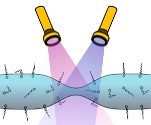
  $\varGamma ^*_{tr}$, respectively. Additionally, the thread is illuminated with a combination of UV and blue light to force switching of the two isomers. A schematic of the considered problem can be seen in figure 1.

Figure 1. Schematic of a section of the infinite thread considered. The thread is illuminated with a combination of UV (tighter squiggles) and blue light (longer squiggles) to force the switch between the two states.
We seek to model, analyse and understand the novel physics supported by this system. The general mathematical model governing the dynamics inside the bulk of the liquid thread is given by the incompressible Navier–Stokes equations
 $$\begin{gather} \boldsymbol{\nabla}\boldsymbol{\cdot}\boldsymbol{u^*} =0, \end{gather}$$
 $$\begin{gather}\rho^*\left(\frac{\partial \boldsymbol{u}^*}{\partial t^*} +\boldsymbol{u}^* \boldsymbol{\cdot} \boldsymbol{\nabla} \boldsymbol{u}^*\right) ={-}\boldsymbol{\nabla} p^*+\mu^* \nabla^{2}\boldsymbol{u}^* \end{gather}$$
and convection–diffusion–reaction equations for the bulk surfactant concentrations
 $$\begin{gather} \frac{\partial c_{tr}^*}{\partial t^*}+\boldsymbol{u}^*\boldsymbol{\cdot}\boldsymbol{\nabla} c_{{tr}}^* =D^*_{{tr}}\nabla^{2}c^*_{{tr}}-k^*_{tr\rightarrow ci}c_{{tr}}^*+k^*_{ci\rightarrow tr}c_{{ci}}^*, \end{gather}$$
 $$\begin{gather}\frac{\partial c_{ci}^*}{\partial t^*}+\boldsymbol{u}^*\boldsymbol{\cdot}\boldsymbol{\nabla} c_{{ci}}^* =D^*_{{ci}}\nabla^{2}c^*_{{ci}}-k^*_{ci\rightarrow tr}c_{{ci}}^*+k^*_{tr\rightarrow ci}c_{{tr}}^*. \end{gather}$$
At the interface  $r^*=S^*(z^*,t^*)$, with outward-pointing unit normal $\boldsymbol {n}^*$, the surface excess (or interfacial surfactant) concentration equations read
 $$\begin{gather} \frac{\partial \varGamma_{tr}^*}{\partial t^*}+\boldsymbol{\nabla}_{s}\boldsymbol{\cdot}\left(\boldsymbol{u}^*\varGamma_{{tr}}^*\right) + \varGamma_{tr}^*\boldsymbol{n}\boldsymbol{\cdot}\left(\boldsymbol{\nabla}_{s}\boldsymbol{\cdot}\boldsymbol{n}\right)\boldsymbol{u}^* =D^*_{{s,tr}}\nabla_{s}^2\varGamma_{{tr}}^*+J_{{tr}}^*-k^*_{s,tr\rightarrow ci}\varGamma_{{tr}}^*+k^*_{s,ci\rightarrow tr}\varGamma_{{ci}}^*,\end{gather}$$
 $$\begin{gather}
\frac{\partial \varGamma_{ci}^*}{\partial t^*}+\boldsymbol{\nabla}_{s}\boldsymbol{\cdot}\left(\boldsymbol{u}^*\varGamma_{{ci}}^*\right)
+ \varGamma_{ci}^*\boldsymbol{n}\boldsymbol{\cdot}\left(\boldsymbol{\nabla}_{s}\boldsymbol{\cdot}\boldsymbol{n}\right)\boldsymbol{u}^*
\,{=}\,D^*_{{s,ci}}\nabla^2_{s}\varGamma_{{ci}}^*\,{+}\,J_{{ci}}^*\,{-}\,k^*_{s,ci\rightarrow
tr}\varGamma_{{ci}}^*\,{+}\,k^*_{s,tr\rightarrow
ci}\varGamma_{{tr}}^*.
\end{gather}$$
$$\begin{gather}
\frac{\partial \varGamma_{ci}^*}{\partial t^*}+\boldsymbol{\nabla}_{s}\boldsymbol{\cdot}\left(\boldsymbol{u}^*\varGamma_{{ci}}^*\right)
+ \varGamma_{ci}^*\boldsymbol{n}\boldsymbol{\cdot}\left(\boldsymbol{\nabla}_{s}\boldsymbol{\cdot}\boldsymbol{n}\right)\boldsymbol{u}^*
\,{=}\,D^*_{{s,ci}}\nabla^2_{s}\varGamma_{{ci}}^*\,{+}\,J_{{ci}}^*\,{-}\,k^*_{s,ci\rightarrow
tr}\varGamma_{{ci}}^*\,{+}\,k^*_{s,tr\rightarrow
ci}\varGamma_{{tr}}^*.
\end{gather}$$
In (2.1)–(2.2),  $\rho ^*$ is the fluid density and $\mu ^*$ its viscosity. Equations (2.3)–(2.4) are surfactant evolution equations that govern bulk concentrations for each isomer. In these equations, the respective diffusion coefficients are denoted by $D^*_{ci}$ and $D^*_{tr}$. The non-negative parameters $k^*_{ci \rightarrow tr}$ and $k^*_{tr \rightarrow ci}$ indicate switching rates from the cis-to-trans and trans-to-cis states, respectively. Switching rates are functions of the intensity of the irradiating light, $I^*_0$, and its wavelength, $\lambda ^*$, as discussed by Shang et al. (Reference Shang, Smith and Hatton2003). For clarity, they can be written in terms of these parameters as
 $$\begin{gather} k^*_{tr \rightarrow ci} \left(\lambda^*,I^*_0\right)= \frac{\epsilon^*_{{tr}}\left(\lambda^*\right) \phi_{{tr-ci}}\lambda^*I_0^*}{N^*_{A}h^*c^*_{{\ell}}}, \end{gather}$$
 $$\begin{gather}k^*_{ci \rightarrow tr}\left(\lambda^*,I^*_0\right) = \frac{\epsilon^*_{{ci}}\left(\lambda^*\right) \phi_{{ci-tr}}\lambda^*I_0^*}{N^*_{A}h^*c^*_{{\ell}}}, \end{gather}$$
where  $I^*_0$ is in units of ${\rm W}\ {\rm m}^{-2}$ as in Chevallier et al. (Reference Chevallier, Mamane, Stone, Tribet, Lequeux and Monteux2011). In general, the light intensity can be a function of space and time; however, for this paper we restrict ourselves to investigating the impact of constant and uniform illumination so that photoisomerization rates are also constant and uniform. In (2.7)–(2.8), the parameters $\epsilon ^*_{{ci}}$ and $\epsilon ^*_{{tr}}$ are the molar extinction coefficients in each reaction, $\phi _{{ci-tr}}$ and $\phi _{{tr-ci}}$ are the corresponding quantum yields, $N^*_{A}$ is Avogadro's constant, $h^*$ is Planck's constant and $c^*_{{\ell }}$ is the speed of light.
The final two equations, (2.5)–(2.6), govern the surface excess of each isomer type and are only valid at the interface,  $r^*=S^*(z^*,t^*)$. They are similar in form to the derivations by Stone (Reference Stone1990), Wong, Rumschitzki & Maldarelli (Reference Wong, Rumschitzki and Maldarelli1996) and Pereira & Kalliadasis (Reference Pereira and Kalliadasis2008), with the addition of the two light-induced switching fluxes. Subscripts $s$ are used to indicate interfacial quantities (for example, $D^*_{{s,ci}}$, etc.), while $\boldsymbol {\nabla }_{s}$ and $\nabla _{s}^2$ denote the surface gradient and surface Laplacian, respectively. The light-switching parameters for the interface are left in their general form as $k^*_{s,ci\rightarrow tr}$ and $k^*_{s,tr\rightarrow ci}$, but usually are taken to be identical to their bulk counterparts. The terms $J^*_{{ci}}$ and $J^*_{{tr}}$ are source terms that capture the kinetic flux of the bulk surfactant $c^*_{{ci}}$ and $c^*_{{tr}}$ onto the interface. Different schemes can be used for the fluxes $J^*_{{ci}}$ and $J^*_{{tr}}$ – see Chang & Franses (Reference Chang and Franses1995). In this study a two-species Langmuir kinetics model is employed, whereby the adsorption of monomers takes into account the total available space on the interface, while the desorption is modelled as if the surfactant were an ideal gas. Under this assumption the kinetic fluxes take the form
 $$\begin{gather} J^*_{{tr}}\left(c^*_{{tr}},\varGamma^*_{{tr}},\varGamma^*_{{ci}}\right) =k_{a}^{tr*}c^*_{{tr}}\left(\varGamma^*_\infty-\varGamma^*_{{ci}}-\varGamma^*_{{tr}}\right)-k_{d}^{tr*}\varGamma^*_{{tr}}, \end{gather}$$
 $$\begin{gather}J^*_{{ci}}\left(c^*_{{ci}},\varGamma^*_{{ci}},\varGamma^*_{{tr}}\right) =k_{a}^{ci*}c^*_{{ci}}\left(\varGamma^*_\infty-\varGamma^*_{{tr}}-\varGamma^*_{{ci}}\right)-k_{d}^{ci*}\varGamma^*_{{ci}}, \end{gather}$$
where the constants  $k_{{a}}^{tr*}$, $k_{{a}}^{ci*}$ are adsorption coefficients and $k_{{d}}^{tr*}$, $k_{{d}}^{ci*}$ are desorption coefficients. This kinetic model is only valid when $\varGamma _\infty ^*$, the maximum packing density, is the same for each isomer type. In general, this is not the case, but certain photosurfactants do display this behaviour (Shang et al. Reference Shang, Smith and Hatton2003). This assumption significantly simplifies the model and will be pursued here, noting that access to the general case is straightforward. The corresponding equation of state to this kinetic scheme, that describes the surface tension coefficient as a function of interfacial surfactant, is given by
 \begin{equation} \gamma^* =\gamma_0^* + nR_{g}^*T^*\varGamma^*_\infty \ln\left(1-\frac{\varGamma^*_{ci}}{\varGamma^*_\infty}-\frac{\varGamma^*_{tr}}{\varGamma^*_\infty}\right),\end{equation}
where  $n$ is a surfactant style constant, $R_{g}^*$ is the universal gas constant and $T^*$ is the absolute temperature.
The surface tension equation (2.11) is used to define boundary conditions through viscous stress balances at  $r^* = S^*(z^*,t^*)$, combining the velocity field and interfacial surfactant concentrations. Separating these into normal and tangential stress balances provides
 \begin{equation} p_{atm}^* + \boldsymbol{n}\boldsymbol{\cdot} \boldsymbol{\tau}^* \boldsymbol{\cdot} \boldsymbol{n} = \gamma^*\kappa^*,\quad \boldsymbol{t}\boldsymbol{\cdot} \boldsymbol{\tau}^* \boldsymbol{\cdot} \boldsymbol{n} = \boldsymbol{t}\boldsymbol{\cdot}\boldsymbol{\nabla}_{s}\gamma^*, \end{equation}
where  $\boldsymbol {\tau }^*=-p^*\boldsymbol {I}+\mu ^*(\boldsymbol {\nabla }\boldsymbol {u}^* +(\boldsymbol {\nabla }\boldsymbol {u}^*)^\intercal )$ is the stress tensor, $p_{atm}^*$ is the constant pressure in the outer fluid, $\boldsymbol {t}$ is unit tangent vector in the $z^*$ direction and $\kappa ^*$ is the mean curvature of the thread surface.
A mass balance couples the bulk surfactant and interfacial surfactant concentrations. It requires that the diffusive flux from the bulk onto the interface balances with the total kinetic flux according to
 \begin{equation} D^*_{tr}\left(\boldsymbol{n}\boldsymbol{\cdot} \boldsymbol{\nabla} c_{tr}^*\right)={-}J^*_{tr}, \quad D^*_{ci}\left(\boldsymbol{n}\boldsymbol{\cdot} \boldsymbol{\nabla} c_{ci}^*\right)={-}J^*_{ci}. \end{equation}
Finally, a kinematic condition is needed at  $r^*=S^*(z^*,t^*)$ to track the shape of the interface. This reads
 \begin{equation} u^* = \frac{\partial S^*}{\partial t^*}+w^*\frac{\partial S^*}{\partial z^*}\end{equation}
and closes the statement of the mathematical model.
We additionally introduce the concept of a maximum depletion length (Cicciarelli, Hatton & Smith Reference Cicciarelli, Hatton and Smith2007) or absorption length (Lin, McKeigue & Maldarelli Reference Lin, McKeigue and Maldarelli1990),  ${L}^*_\infty =\varGamma _\infty ^*/c_0^*$. In Cartesian coordinates this length is the depth of a liquid layer at concentration $c_0^*$ that contains enough surfactant to fill an interface at concentration $\varGamma _\infty ^*$. It is small when there is much bulk surfactant and large when there is not. A cylindrical extension to this is the definition of a depletion radius, $\mathcal {R}^*_\infty$, which is the inner radius of an annulus of liquid with outer radius $R^*$ and concentration $c_0^*$ that contains enough surfactant to fill the interface at the maximum packing density. The geometry leads to the definition
 \begin{equation} \mathcal{R}^*_\infty=\sqrt{R^{*2}-2R^*{L}^*_\infty} \end{equation}
so that it approaches  $R^*$ when ${L}^*_\infty$ is small. This parameter is notably complex for ${L}^*_\infty >0.5R^*$ when there is not enough surfactant in the bulk to saturate a clean interface. These two parameters are not independent in the formulation, but can be helpful in discussing the physics of the problem.
Before moving to the dimensionless formulation it should be noted that the above description of surfactant transport has many similarities with that of charge transport in leaky dielectric fluids as per the canonical review by Melcher & Taylor (Reference Melcher and Taylor1969).
3. Dimensionless formulation
Prior to our theoretical investigation, we non-dimensionalize the equations as follows. Lengths are scaled by the undisturbed thread radius  $R^*$; velocities are scaled with the capillary scaling $U^*=\gamma _0^*/\mu ^*$, time by $R^*\mu /\gamma _0^*$, bulk surfactant concentrations $c^*_{{ci}}$ and $c^*_{{tr}}$ are scaled with a typical uniform value $c^*_0$, interfacial concentrations $\varGamma ^*_{{ci}}$ and $\varGamma ^*_{{tr}}$ are scaled with $\varGamma _\infty ^*$, and the pressure $p^*$ (taken relative to $p_{atm}^*$) and stress tensor $\boldsymbol {\tau }^*$ are scaled by $\gamma _0^*/R^*$. Here, $c^*_0$ is taken to be the average total concentration of surfactant in the bulk of the fluid. As a final step, and in the interest of reducing the number of parameters rather than any technical barriers, we assume that the rate of switching due to irradiated light is identical in the bulk and on the interface.
This results in the following dimensionless set of equations, where variables without asterisks are dimensionless but otherwise correspond to the same dependent and independent variables as before. The numerous dimensionless parameters that emerge will be discussed in detail below. Equations (2.1)–(2.6) become
 $$\begin{gather} \boldsymbol{\nabla}\boldsymbol{\cdot}\boldsymbol{u} =0, \end{gather}$$
 $$\begin{gather}{Re}\left(\frac{\partial \boldsymbol{u}}{\partial t}+\boldsymbol{u} \boldsymbol{\cdot} \boldsymbol{\nabla} \boldsymbol{u}\right) ={-}\boldsymbol{\nabla} p+\nabla^{2}\boldsymbol{u}, \end{gather}$$
 $$\begin{gather}\frac{\partial c_{tr}}{\partial t}+\boldsymbol{u}\boldsymbol{\cdot}\boldsymbol{\nabla} c_{{tr}} =\frac{1}{{Pe}_{{tr}}}\nabla^{2}c_{{tr}}-{Da}_{tr} c_{{tr}}+{Da}_{ci} c_{{ci}}, \end{gather}$$
 $$\begin{gather}\frac{\partial c_{ci}}{\partial t}+\boldsymbol{u}\boldsymbol{\cdot}\boldsymbol{\nabla} c_{{ci}} =\frac{1}{{Pe}_{{ci}}}\nabla^{2}c_{{ci}}-{Da}_{ci} c_{{ci}}+{Da}_{tr} c_{{tr}}, \end{gather}$$
 $$\begin{gather}\frac{\partial \varGamma_{tr}}{\partial t}+\boldsymbol{\nabla}_{s}\boldsymbol{\cdot}\left(\boldsymbol{u}\varGamma_{{tr}}\right) + \varGamma_{tr} \boldsymbol{n}\boldsymbol{\cdot}\left(\boldsymbol{\nabla}_{s}\boldsymbol{\cdot}\boldsymbol{n}\right)\boldsymbol{u} =\frac{1}{{Pe}_{{s,tr}}}\nabla_{s}^2\varGamma_{{tr}} +J_{{tr}}-{Da}_{s,tr}\varGamma_{{tr}}+{Da}_{s,ci}\varGamma_{{ci}}, \end{gather}$$
 $$\begin{gather}\frac{\partial \varGamma_{ci}}{\partial t}+\boldsymbol{\nabla}_{s}\boldsymbol{\cdot}\left(\boldsymbol{u}\varGamma_{{ci}}\right) + \varGamma_{ci}\boldsymbol{n}\boldsymbol{\cdot}\left(\boldsymbol{\nabla}_{s}\boldsymbol{\cdot}\boldsymbol{n}\right)\boldsymbol{u} =\frac{1}{{Pe}_{{s,ci}}}\nabla^2_{s}\varGamma_{{ci}} +J_{{ci}}-{Da}_{s,ci}\varGamma_{{ci}}+{Da}_{s,tr}\varGamma_{{tr}}. \end{gather}$$
Defining  $\boldsymbol {e}_r=(1,0,0)$ and $\boldsymbol {e}_z=(0,0,1)$, the normal and tangential vectors read
 \begin{equation} \boldsymbol{n}=\frac{\boldsymbol{e}_{r} - S_z\boldsymbol{e}_{z}}{\sqrt{1 + S_z^2}}, \quad \boldsymbol{t}=\frac{S_z\boldsymbol{e}_{r} + \boldsymbol{e}_{z}}{\sqrt{1 + S_z^2}}. \end{equation}
The kinetic schemes (2.9)–(2.10) become
 $$\begin{gather} J_{{tr}}(c_{{tr}},\varGamma_{{tr}},\varGamma_{{ci}}) ={Bi}_{{tr}}\left[{k}_{{tr}}c_{{tr}}(1-\varGamma_{{tr}}-\varGamma_{{ci}})-\varGamma_{{tr}}\right], \end{gather}$$
 $$\begin{gather}J_{{ci}}(c_{{ci}},\varGamma_{{ci}},\varGamma_{{tr}}) ={Bi}_{{ci}}\left[{k}_{{ci}}c_{{ci}}(1-\varGamma_{{tr}}-\varGamma_{{ci}})-\varGamma_{{ci}}\right], \end{gather}$$
while the equation of state (2.11) is given by
 \begin{equation} \gamma = 1+{Ma}\ln\left(1-\varGamma_{ci}-\varGamma_{tr}\right).\end{equation}
This is used in the normal and tangential stress balances that become
 \begin{equation} \boldsymbol{n}\boldsymbol{\cdot} \boldsymbol{\tau} \boldsymbol{\cdot} \boldsymbol{n} = \gamma\kappa,\quad \boldsymbol{t}\boldsymbol{\cdot} \boldsymbol{\tau} \boldsymbol{\cdot} \boldsymbol{n} = \boldsymbol{t}\boldsymbol{\cdot}\boldsymbol{\nabla}_{s}\gamma, \end{equation}
where  $\boldsymbol {\tau }=-pI+\boldsymbol {\nabla }\boldsymbol {u} +(\boldsymbol {\nabla } \boldsymbol {u})^\intercal$. The interfacial mass balances are now
 \begin{equation} \frac{{k}_{tr}\chi_{tr}}{{Pe}_{tr}}\left(\boldsymbol{n}\boldsymbol{\cdot} \boldsymbol{\nabla} c_{tr}\right)={-}J_{tr}, \quad \frac{{k}_{ci}\chi_{ci}}{{Pe}_{ci}}\left(\boldsymbol{n}\boldsymbol{\cdot} \boldsymbol{\nabla} c_{ci}\right)={-}J_{ci} \end{equation}
and the kinematic condition becomes
 \begin{equation} u = \frac{\partial S}{\partial t} + w\frac{\partial S}{\partial z}.\end{equation}
 The dimensionless parameters merit detailed discussion. The Reynolds number  ${Re}= \rho ^* U^* R^*/\mu ^*$, the Péclet numbers (e.g. ${Pe}_{{ci}}=U^*R^*/D^*_{{ci}}$) and the interfacial Péclet numbers (e.g. ${Pe}_{{s},{ci}}=U^*R^*/D^*_{{s,ci}}$) are defined as is typical, comparing inertia with viscous forces in the case of $Re$ and advection to diffusion in the bulk and at the interface, respectively, in the cases of the two Péclet numbers. In the surfactant equations, Damköhler numbers are defined that compare switching rates with advective fluxes. These are given by
 \begin{equation} {Da}_{{tr}} = \frac{k_{tr\rightarrow ci}^* R^*}{U^*},\quad {Da}_{{ci}} = \frac{k_{ci\rightarrow tr}^*R^*}{U^*}, \end{equation}
for trans-to-cis reactions and cis-to-trans reactions, respectively. Likewise, the surface Damköhler numbers are given by
 \begin{equation} {Da}_{{s},{tr}} = \frac{k_{s,tr\rightarrow ci}^* R^*}{U^*},\quad {Da}_{{s},{ci}} = \frac{k_{s,ci\rightarrow tr}^*R^*}{U^*}, \end{equation}
but are usually assumed to be identical to their bulk counterparts. The Biot numbers, encountered in the definition of kinetic flux, are defined by
 \begin{equation} {Bi}_{ci}= \frac{k_{{d}}^{{ci}*}R^*}{U^*},\quad {Bi}_{tr}= \frac{k_{{d}}^{{tr}*}R^*}{U^*}, \end{equation}
for cis-type, and trans-type surfactants, respectively. The Biot numbers represent the ratio of kinetic desorption to advective flux. Notably, when a Biot number is zero, the insoluble limit is obtained. The normalized bulk concentrations for cis-type and trans-type surfactants are given by
 \begin{equation} {k}_{{ci}}=\frac{k_{{a}}^{{ci}*}c^*_{0}}{k_{{d}}^{{ci}*}},\quad {k}_{{tr}}=\frac{k_{{a}}^{{tr}*}c^*_{0}}{k_{{d}}^{{tr}*}} \end{equation}
and compare the relative importance of adsorption rate with desorption. The Marangoni number compares the stress due to gradients in surface tension with the viscous stresses in the fluid and is given by
 \begin{equation} {Ma} = \frac{nR_{g}^*T^*\varGamma_\infty^*}{\mu^*U^*}. \end{equation}
The following kinetic parameters also enter:
 \begin{equation} \chi_{{ci}}=k_{{d}}^{{ci}*}R^*/\kern0.1pt\big(k_{{a}}^{{ci}*}\varGamma^*_{\infty}\big),\quad \chi_{{tr}}=k_{{d}}^{{tr}*}R^*/\!\left(k_{{a}}^{{tr}*}\varGamma^*_{\infty}\right) \end{equation}
and upon inspection we have the relationship
 \begin{equation} \chi_{{ci}}{k}_{{ci}} = \chi_{{tr}}{k}_{{tr}}={L}_{{\infty}}^{{-}1}, \end{equation}
where  ${L}_{{\infty }}=\varGamma ^*_\infty /(R^*c^*_0)$ is the dimensionless maximum adsorption length or depletion thickness. In Cartesian coordinates this length would refer to the fraction of the domain required to fill the interface. Its cylindrical extension, the dimensionless depletion radius, becomes
 \begin{equation} \mathcal{R}_\infty = \sqrt{1-2L_\infty} \end{equation}
and like  $L_\infty$, it is related to the fraction of the surfactant in the domain required to fill the interface. For values below $L_\infty =0.5$, as $L_\infty$ gets smaller (or $\chi _{{ci}}{k}_{{ci}}$ and $\chi _{{tr}}{k}_{{tr}}$ grow larger), $\mathcal {R}_\infty$ approaches 1, meaning the fraction of the total surfactant in the bulk required to fill up the interface decreases. Conversely as $L_\infty \rightarrow \infty$, $\mathcal {R}_\infty \rightarrow 0$ and then becomes complex indicating the entirety of the bulk surfactant could not fit on the interface. A list of the dimensionless parameters can be found in table 1. Any trans-type dimensionless parameters not mentioned explicitly in the text are identical to their cis-type counterparts after swapping the subscripts from ‘ci’ to ‘tr’.
Table 1. Dimensionless parameters used in the problem statement. Any trans-type dimensionless parameters are identical in form to their cis-type counterparts after swapping the subscripts from ‘ $ci$’ to ‘ $tr$’. The last column covers the range of values used in the results section. The values for ${k}_{tr}$, ${Bi}_{tr}$ and ${\chi }_{tr}$ differ slightly from the cis-type values as per § 4.1. Abbreviations used: advection (adv.); diffusion (diff.).

Our objective is to study the linear stability of this intricate physical system. Unlike single species surfactant systems that support uniform trivial base states, the present multispecies system allows radially non-uniform surfactant distributions that have a significant impact on flow stability. We analyse permissible base states next before moving on to their stability.
4. The undisturbed states
To calculate the base states we consider a motionless, perfectly cylindrical thread of radius  $r=1$ under constant and uniform illumination. The last assumption implies that the light induced switching rates are precisely captured by the two Damköhler numbers, ${Da}_{ci}$ and ${Da}_{tr}$. With these assumptions the concentration profiles become uniform in the $z$-direction and all gradients in that direction vanish, creating a so called photostationary state. Then, if we denote base state variables with a bar, the unknowns to be calculated are the radially dependent bulk surfactant concentrations $\bar {c}_{{tr}}(r)$ and $\bar {c}_{{ci}}(r)$, and the constant interfacial surfactant concentrations $\bar {\varGamma }_{tr}$ and $\bar {\varGamma }_{ci}$. The equations in the bulk ((3.1)–(3.4) in the absence of fluid flow) reduce to
 $$\begin{gather} \frac{1}{{Pe}_{tr}}\frac{1}{r}\frac{\mathrm{d}}{\mathrm{d}r} \left(r\frac{\mathrm{d}\bar{c}_{{tr}}}{\mathrm{d}r}\right) ={-}{Da}_{ci}\bar{c}_{{ci}} +{Da}_{tr}\bar{c}_{{tr}}, \quad 0< r<1,\end{gather}$$
 $$\begin{gather}\frac{1}{{Pe}_{ci}}\frac{1}{r}\frac{\mathrm{d}}{\mathrm{d}r} \left(r\frac{\mathrm{d}\bar{c}_{{ci}}}{\mathrm{d}r}\right)={Da}_{ci}\bar{c}_{{ci}} -{Da}_{tr}\bar{c}_{{tr}}, \quad 0< r<1. \end{gather}$$
These must be solved subject to the steady-state boundary conditions coming from (3.5)–(3.6), and the kinetic schemes (3.8)–(3.9) that read, on  $r=1$,
 $$\begin{gather} {Da}_{s,ci}\bar{\varGamma}_{ci}-{Da}_{s,tr}\bar{\varGamma}_{tr}={-}\frac{\chi_{ci}{k}_{ci}}{{Pe}_{ci}}\frac{\mathrm{d}\bar{c}_{ci}}{\mathrm{d}r}, \end{gather}$$
 $$\begin{gather}-{Da}_{s,ci}\bar{\varGamma}_{ci}+{Da}_{s,tr}\,\bar{\varGamma}_{tr} ={-}\frac{\chi_{tr}{k}_{tr}}{{Pe}_{tr}}\frac{\mathrm{d}\bar{c}_{tr}}{\mathrm{d}r}, \end{gather}$$
 $$\begin{gather}\frac{\chi_{tr}{k}_{tr}}{{Pe}_{tr}}\frac{\mathrm{d}\bar{c}_{tr}}{\mathrm{d}r} ={-}{Bi}_{tr}\left[{k}_{tr}\,\bar{c}_{tr}\left(1-\bar{\varGamma}_{ci}-\bar{\varGamma}_{tr}\right)-\bar{\varGamma}_{tr}\right], \end{gather}$$
 $$\begin{gather}\frac{\chi_{ci}{k}_{ci}}{{Pe}_{ci}}\frac{\mathrm{d}\bar{c}_{ci}}{\mathrm{d}r} ={-}{Bi}_{ci}\left[{k}_{ci}\,\bar{c}_{ci}\left(1-\bar{\varGamma}_{ci}-\bar{\varGamma}_{tr}\right)-\bar{\varGamma}_{ci}\right]. \end{gather}$$
The details of the solution of the above equations are discussed in Appendix A. It is shown that the solutions for  $\bar {c}_{tr}$ and $\bar {c}_{ci}$ take the form
 $$\begin{gather} \bar{c}_{tr}(r)=\frac{\eta C_0 {\rm I}_0(\sqrt{\zeta}r)+\alpha M}{\eta + \alpha}, \end{gather}$$
 $$\begin{gather}\bar{c}_{ci}(r)=\frac{M-C_0 {\rm I}_0(\sqrt{\zeta}r)}{\eta + \alpha}, \end{gather}$$
where  ${\rm I}_0$ is the zeroth-order modified Bessel function, $C_0$ is a constant determined from conditions on the interface and $M$ is a controllable parameter related to the total amount of surfactant in the system. If the Péclet numbers are the same, then $M$ is the dimensionless total amount of surfactant in the bulk and therefore necessarily equal to 1. The parameters $\alpha$ and $\eta$ represent the ratios of Damköhler and Péclet numbers, and $\zeta$ is a parameter involving both Damköhler and Péclet numbers, given by
 \begin{equation} \alpha=\frac{{Da}_{ci}}{{Da}_{tr}},\quad\eta=\frac{{Pe}_{tr}}{{Pe}_{ci}}, \quad\zeta={Da}_{ci}{Pe}_{ci}+{Da}_{tr}{Pe}_{tr}={Da}_{tr}{Pe}_{ci}(\alpha+\eta). \end{equation}
It is important to note that these solutions necessarily satisfy the following mass balance throughout the liquid thread:
 \begin{equation} \frac{\chi_{tr}{k}_{tr}}{{Pe}_{tr}}\frac{\mathrm{d}\bar{c}_{tr}}{\mathrm{d}r} ={-}\frac{\chi_{ci}{k}_{ci}}{{Pe}_{ci}}\frac{\mathrm{d}\bar{c}_{ci}}{\mathrm{d}r}.\end{equation}
Physically this means that at all locations in the domain the diffusive flux of one species is exactly equal and opposite to that of the other species. It follows from (4.5)–(4.6) that the interfacial surfactants can be written in terms of these bulk concentrations as follows:
 \begin{gather} \bar{\varGamma}_{tr}=\frac{\left(\dfrac{1}{{Bi}_{tr}}+\dfrac{{k}_{ci}\bar{c}_{ci}}{{Bi}_{tr}} +\dfrac{{k}_{tr}\bar{c}_{tr}}{{Bi}_{ci}}\right)\dfrac{\chi_{tr}{k}_{tr}}{{Pe}_{tr}} \dfrac{\mathrm{d}\bar{c}_{tr}}{\mathrm{d}r} + {k}_{tr}\bar{c}_{tr}}{1+{k}_{ci}\bar{c}_{ci}+{k}_{tr}\bar{c}_{tr}}, \end{gather}
 \begin{gather} \bar{\varGamma}_{ci}=\frac{\left(\dfrac{1}{{Bi}_{ci}}+\dfrac{{k}_{ci}\bar{c}_{ci}}{{Bi}_{tr}} +\dfrac{{k}_{tr}\bar{c}_{tr}}{{Bi}_{ci}}\right)\dfrac{\chi_{ci}{k}_{ci}}{{Pe}_{ci}}\dfrac{\mathrm{d}\bar{c}_{ci}}{\mathrm{d}r} + {k}_{ci}\bar{c}_{ci}}{1+{k}_{ci}\bar{c}_{ci}+{k}_{tr}\bar{c}_{tr}}.\end{gather}
Inserting the solutions (4.7)–(4.8) into (4.11)–(4.12) enables the explicit determination of  $C_0$ (see Appendix A for details). This constant is a rather complicated function of the many dimensionless parameters, but can be viewed in a simple way as a coefficient related to the rate of diffusion of the two isomer species onto and off of the interface. It is in general non-zero because of the steady state requirement that the light-switching rate balances the adsorption rate, thereby forcing diffusion onto and off of the interface. The existence of a non-uniform base case is typically not considered when studying photostationary states, i.e. in the use of typical surfactant isotherm models to estimate surface tension in Shang et al. (Reference Shang, Smith and Hatton2003) and Chevallier et al. (Reference Chevallier, Mamane, Stone, Tribet, Lequeux and Monteux2011). The counter diffusion of our two species affects the amount of each isomer on the interface, possibly throwing into doubt the values of the fitting parameters determined in those studies.
4.1. Example solutions for the base state
Given the large number of parameters present in the model, we focus our theoretical efforts by identifying physically relevant cases motivated by previous experimental investigations. Chevallier et al. (Reference Chevallier, Mamane, Stone, Tribet, Lequeux and Monteux2011) provide many of the required parameters, and these are reported in table 2.
Table 2. Representative parameter values taken from Chevallier et al. (Reference Chevallier, Mamane, Stone, Tribet, Lequeux and Monteux2011). Relevant to this manuscript are the ratios of the adsorption and desorption coefficients and that the diffusion coefficients are equal.

Of particular interest are the ratios of the adsorption and desorption coefficients, which are seen to be
 \begin{equation} \frac{k_{{a}}^{{ci}*}}{k_{{a}}^{{tr}*}} \approx 10, \quad \frac{k_{{d}}^{{ci}*}}{k_{{d}}^{{tr}*}} \approx 300. \end{equation}
This implies that even though the adsorption of cis-type isomers is faster than trans-type ones, the desorption rate is much greater, leading to a preference of cis-type isomers to leave the interface. Mathematically, this difference in kinetic behaviour dictates values of  ${Bi}_{ci}$ to be 300 times larger than those of ${Bi}_{tr}$, while at the same time ${k}_{tr}$ is 30 times larger than ${k}_{ci}$. Subsequently, due to (3.20), we find that $\chi _{ci}$ is 30 times larger than $\chi _{tr}$. Using these fixed ratios reduces these six parameter choices to three, namely ${Bi}_{ci}$, ${k}_{ci}$ and $\chi _{ci}$, and hence simplifying the parameter space while maintaining salient essential physical characteristics of the system. Crucially, the Peclét numbers are now the same, implying $\eta =1$ and $M=1$, and we additionally make the assumption that the bulk Damköhler numbers and surfaces ones are identical.
A first parameter of interest is the size of the reaction–diffusion layer at the interface. If this layer is thin, i.e. when diffusion is slow, we denote the width of this region as  $\delta$ and by balancing diffusion and the reactions terms in the bulk equations it can be shown that
 \begin{equation} \delta\sim\zeta^{{-}1/2}, \end{equation}
which is unsurprisingly the inverse of the argument of the Bessel functions in (4.7) and (4.8). It also could be expected since  $\zeta$ is linear in both Péclet numbers ${Pe}_{{tr}}$ and ${Pe}_{{ci}}$, and hence $\delta \sim {Pe}_{{tr}}^{-1/2}\sim {Pe}_{{ci}}^{-1/2}$ if both are large. To confirm this relationship we calculated a numerical $\delta$ value from the exact solution. It was defined when $\eta =1$ as the distance from the interface at which $\bar {c}_{tr}$ and $\bar {c}_{ci}$ have changed by $99$ per cent of the difference between their values at $r=1$ and $r=0$. Explicitly, $\delta$ is such that
 \begin{equation} \bar{c}_{tr}(r=1-\delta)=\bar{c}_{tr}(r=0)+0.01\left[\bar{c}_{tr}(r=1)-\bar{c}_{tr}(r=0)\right]. \end{equation}
Figure 2 shows the solution to this equation for a range of  $\zeta$ values, showing the expected negative square root behaviour at larger values of $\zeta$.

Figure 2. Relationship between  $\zeta$ and $\delta$. For all panels ${Bi}_{ci}=10^3$, ${Bi}_{tr}=3.33$, $\chi _{ci}=1$, $\chi _{tr}=30$ and ${Pe}_{tr}={Pe}_{ci}=10$.
Additionally, figure 2 contains some illustrative plots displaying the effect of varying the Damköhler numbers and normalized bulk surfactants on the undisturbed states. To help explain them we begin with a discussion of the impact of the Damköhler numbers.
Figure 2(a,b) have the same value of  $\zeta =110$, but different values of Damköhler numbers, with figure 2(a) having ${Da_{tr}}>{Da_{ci}}$ and figure 2(b) the opposite. The differing Damköhler numbers are important in setting the relative amount of each surfactant. For example, in figure 2(a) when ${Da_{tr}}>{Da_{ci}}$ there are significantly more cis isomers than trans (recall $\bar {c}_{ci}+\bar {c}_{tr}=1$), while the opposite is true in figure 2(b). This can be attributed to the solutions in (4.7) and (4.8) which reveal that for small enough values of $\delta$ then as $r\rightarrow 0$ the bulk concentrations tend to
 \begin{equation} \bar{c}_{tr} = \frac{{Da}_{ci}}{{Da}_{ci}+{Da}_{tr}}, \quad \bar{c}_{ci} = \frac{{Da}_{tr}}{{Da}_{ci}+{Da}_{tr}}, \end{equation}
a limiting behaviour which can be seen in all the panels of figure 2 as  $r\rightarrow 0$. Figure 2(c) shows a case with a larger value of $\zeta$, but equal Damköhler numbers. Consequently, $\delta$ is smaller (the diffusion layer is thinner) than in figures 2(a) and 2(b), but $\bar {c}_{ci}$ tends to 0.5 as $r\rightarrow 0$.
Figure 2(a–c) also show the impact of increasing the normalized bulk concentration,  ${k}_{ci}$. Since this is the only parameter that contains $c_0^*$ (the dimensional average total surfactant concentration) in our problem set-up, this can be viewed as increasing the amount of surfactant in the system. In all cases, we observe that as ${k}_{ci}$ increases, the solution tends to the constant far field value everywhere. This happens because as ${k}_{ci}\rightarrow \infty$, it necessarily follows that $\mathrm {d} \bar {c}_{ci}/\mathrm {d} r \rightarrow 0$, so that the interfacial surfactant equations remain bounded. Therefore, the coefficient $C_0\rightarrow 0$. The physical reason for this behaviour is that as ${k}_{ci}$ increases, adsorption dominates over desorption, but at the same time the interface becomes saturated, thereby also shutting off the driving force for adsorption. Since there is no adsorption or desorption there can be no diffusive flux to or from the interface, and the bulk equations yield constant uniform states. This can be understood in another way in the context of $\mathcal {R}_\infty$, the depletion radius. As ${k}_{ci}$ increases with $\chi _{ci}$ held constant, $\mathcal {R}_\infty$ approaches 1. This essentially means there is much surfactant very close to the interface in the bulk. Therefore, any kinetic fluxes onto or off the meniscus will do little to change bulk surfactant distributions, leading to near constant values of the bulk solutions in $r$.
$r$.
The saturation of the interface as  ${k}_{ci}$ increases is shown in figure 3(a) which plots the total interfacial surfactant (defined to be $\bar {\varGamma }_{tot} =\bar {\varGamma }_{ci}+\bar {\varGamma }_{tr}$), as a function of ${k}_{ci}$ for four different combinations of Damköhler numbers. It is seen that for all cases the interface becomes completely saturated with surfactant as ${k}_{ci}\rightarrow \infty$. However, before complete saturation is reached, the choice of Damköhler numbers has a large effect on interfacial surfactant levels as we discuss next. When ${Da}_{ci}$ and ${Da}_{tr}$ are equal, e.g. the solid black and red curves corresponding to ${Da}_{ci}={Da}_{tr}=1$ and ${Da}_{ci}={Da}_{tr}=10$, respectively, there are similar amounts of interfacial surfactants on the interface, with the larger Damköhler case showing only slightly less amounts. The interfacial surfactant concentrations are nearly identical because similar amounts of the two surfactants are present in the system. The small difference can be attributed to an increase in the diffusion rates of the two isomers at larger values of Damköhler numbers due to the decrease in the size of the reaction–diffusion layer. To help explain this phenomenon, it is helpful to look at the analytical form of the base-case interfacial surfactants. It is easily shown by adding $\bar {\varGamma }_{tr}$ and $\bar {\varGamma }_{ci}$ ((4.11) and (4.12)) that
 \begin{equation} \bar{\varGamma}_{tot} = \frac{{k_{ci}}\bar{c}_{ci}+{k_{tr}}\bar{c}_{tr}+\dfrac{\chi_{ci}{k_{ci}}}{{Bi_{ci}} {Pe_{ci}}}\dfrac{\mathrm{d} \bar{c}_{ci}}{\mathrm{d} r} + \dfrac{\chi_{tr}{k_{tr}}}{{Bi_{tr}}{Pe_{tr}}}\dfrac{\mathrm{d} \bar{c}_{tr}}{\mathrm{d} r}}{1+{k_{ci}}\bar{c}_{ci}+{k_{tr}}\bar{c}_{tr}}, \end{equation}
where the two terms with gradients are the mass fluxes from the bulk and capture the impact of the non-uniform solutions for the bulk surfactant distributions on  $\bar {\varGamma }_{ci}$ and $\bar {\varGamma }_{tr}$. From this expression we can infer the role of the mass flux.

Figure 3. Plot of total interfacial surfactant concentration for a base case as a function of  ${k}_{ci}$ for four cases of Damköhler numbers. In this graph $30{k}_{ci}={k}_{tr}$, ${Bi}_{ci}=10^3$, ${Bi}_{tr}=3.33$, $\chi _{ci}=1$, $\chi _{tr}=30$ and ${Pe}_{tr}={Pe}_{ci}=10$.
First, using (4.10) and the fact that  ${Bi_{ci}}>{Bi_{tr}}$, we know the trans flux term will have a greater impact on $\bar {\varGamma }_{tot}$ than the cis flux term. The direction of diffusion of both species (and therefore the sign of $C_0$) is thus crucial to determining whether the mass fluxes are adding or subtracting from the total surfactant on the interface. It is shown in Appendix A that for the parameter set we are considering, and assuming that the surface Damköhler numbers and bulk ones are the same, $C_0$ is always negative. This means that at steady state cis isomers will always have a net desorption off the interface and trans isomers will have a net adsorption on to the interface, a claim supported by the subplots in figure 2. Returning to (4.17), we know $\mathrm {d}\bar {c}_{ci}/\mathrm {d}r>0$ and $\mathrm {d}\bar {c}_{tr}/\mathrm {d}r<0$ by (4.10), meaning the mass fluxes reduce the total interfacial surfactant due to the ordering ${Bi_{ci}}>{Bi_{tr}}$. This is reflected in figure 3 when $\bar {\varGamma }_{tot}$ decreases as the Damköhler numbers increase from ${Da}_{{ci}}={Da}_{{tr}}=1$ to ${Da}_{{ci}}={Da}_{{tr}}=10$.
For the cases when  ${Da}_{ci}\neq {Da}_{tr}$, figure 3(b,c) shows larger values of cis concentrations on the interface when ${Da}_{tr}$ is greater than ${Da}_{ci}$ and larger values of trans concentrations on the interface when the opposite is true. This can be attributed to the bulk values of each species in each case. However, because ${k}_{tr}$ is much larger than ${k}_{ci}$, the impact of these two states on the surface tension is quite different. This means trans isomers are much more likely to stay attached to the interface than the cis isomers. As a consequence, when ${Da}_{ci}$ is greater than ${Da}_{tr}$ there are significantly higher total interfacial concentrations at lower values of ${k}_{ci}$ than when ${Da}_{tr}$ is greater than ${Da}_{ci}$, as seen in figure 3(a). Physically this means that for a given bulk surfactant concentration, illumination with more blue light than UV radiation ( ${Da}_{ci}>{Da}_{tr}$) leads to more surface excess, while more UV illumination than blue ( ${Da}_{ci}<{Da}_{tr}$) leads to less. This ability to control surface excess through light gives a clear technological pathway to the control of surface tension.
4.2. Summary of the undisturbed states
The considered reaction–diffusion problem displays a radially non-uniform steady state that arises because photoswitching of the surfactants on the interface ensures that the surfactants fail to reach equilibrium (namely zero diffusion) at the interface. The result is two counter-diffusing species, where one species is adsorbing onto the interface and the other is desorbing at an equal rate. The amount of each type of surfactant in the system is generally determined by the ratio of the Damköhler numbers as given by (4.16a,b). The values of  $\zeta$ and $C_0$ are important parameters that affect the gradient of surfactants in the bulk; here $\zeta$ determines the size of the reaction–diffusion layer, and $C_0$ is a complicated function of every dimensionless parameter in the problem and multiplies the gradients. When ${k}_{tr}>{k}_{ci}$, but ${Bi}_{tr}<{Bi}_{ci}$, as is the case with the surfactants in Chevallier et al. (Reference Chevallier, Mamane, Stone, Tribet, Lequeux and Monteux2011), $C_0$ is always negative. This means that for all parameter sets cis isomers desorb off the interface and trans isomers adsorb onto the interface. With this undisturbed state in mind, we now turn to hydrodynamic stability aspects with particular interest on the effect of chromocapillary mechanisms on classical Rayleigh–Plateau instabilities.
5. Linear stability
We consider small axisymmetric perturbations to the undisturbed quiescent cylindrical liquid thread and corresponding radial distribution of the two surfactant species analysed in the previous section. Additionally, we assume that the thread is in the Stokes regime ( $Re=0$). The interface is perturbed by writing $r=1+\epsilon \hat {S}\exp ({\rm i}kz+{\rm i}st)+{\rm c.c.}$ where $\epsilon \ll 1$ is infinitesimally small, $\hat {S}$ is a constant and ${\rm c.c.}$ denotes the complex conjugate of the preceding term. We also write $\phi (r,z,t) =\bar {\phi }(r) + \epsilon \hat {\phi }(r)\exp ({\rm i}kz+{\rm i}st)+{\rm c.c.}$, where $\phi$ can be any of our dependent variables, and it is understood that bars correspond to the steady basic states calculated previously. Plugging this into our system of (3.1)–(3.6) and linearizing with respect to $\epsilon$, yields the linear system
 $$\begin{gather} \frac{\mathrm{d} \hat{u}}{\mathrm{d} r }+\frac{1}{r}\hat{u} + {\rm i}k\hat{w} = 0, \end{gather}$$
 $$\begin{gather}\widehat{\boldsymbol{\nabla}}^2 \hat{u} -\frac{1}{r^2}\hat{u} = \frac{\mathrm{d} \hat{p}}{\mathrm{d} r}, \end{gather}$$
 $$\begin{gather}\widehat{\boldsymbol{\nabla}}^2 \hat{w} = {\rm i}k\hat{p}, \end{gather}$$
 $$\begin{gather}s\hat{c}_{ci} +\hat{u}\frac{\mathrm{d}\bar{c}_{ci}}{\mathrm{d}r} =\frac{1}{{Pe}_{{ci}}}\widehat{\boldsymbol{\nabla}}^2\hat{c}_{{ci}}-{Da}_{ci}\hat{c}_{{ci}}+{Da}_{tr}\hat{c}_{{tr}}, \end{gather}$$
 $$\begin{gather}s\hat{c}_{tr} +\hat{u}\frac{\mathrm{d}\bar{c}_{tr}}{\mathrm{d}r} =\frac{1}{{Pe}_{{tr}}}\widehat{\boldsymbol{\nabla}}^2\hat{c}_{{tr}}-{Da}_{tr}\hat{c}_{{tr}}+{Da}_{ci}\hat{c}_{{ci}}, \end{gather}$$
 $$\begin{gather}s\hat{\varGamma}_{ci}+{\rm i}k{\hat{w}}\bar{\varGamma}_{{ci}} + \hat{u}\bar{\varGamma}_{ci} ={-}\frac{k^2}{{Pe}_{{s,ci}}}\hat{\varGamma}_{{ci}}+\hat{J}_{{ci}}-{Da}_{ci}\hat{\varGamma}_{{ci}}+{Da}_{tr}\hat{\varGamma}_{{tr}}, \end{gather}$$
 $$\begin{gather}s \hat{\varGamma}_{tr}+{\rm i}k{\hat{w}}\bar{\varGamma}_{{tr}}+ \hat{u}\bar{\varGamma}_{tr} ={-}\frac{k^2}{{Pe}_{{s,tr}}}\hat{\varGamma}_{{tr}}+\hat{J}_{{tr}}-{Da}_{tr}\hat{\varGamma}_{{tr}}+{Da}_{ci}\hat{\varGamma}_{{ci}}, \end{gather}$$
where
 \begin{equation} \widehat{\boldsymbol{\nabla}}^2 = \frac{\mathrm{d}^2 }{\mathrm{d} r^2}+ \frac{1}{r}\frac{\mathrm{d}}{\mathrm{d} r} -k^2. \end{equation}
Here the assumption that the bulk and surface Damköhler numbers are equal has been applied. We note that a Taylor expansion at  $r=1$ has been carried out to arrive at (5.6) and (5.7), and an analogous expansion is used for boundary conditions (3.11a,b), (3.12a,b) and (3.13). It follows that the linearized form of the normal and tangential stress balances (3.11a,b) reads
 \begin{equation}
\hat{p}-2\frac{\mathrm{d} \hat{u}}{\mathrm{d} r} =
\bar{\gamma}\,\big(-\hat{S}+k^2\hat{S}\big)+\hat{\gamma},\quad
\frac{\mathrm{d} \hat{w}}{\mathrm{d} r}+{\rm i}k\hat{u}
={-}\frac{{\rm
i}k{Ma}}{1-\bar{\varGamma}_{ci}-\bar{\varGamma}_{tr}}\,\big(
\hat{\varGamma}_{ci} + \hat{\varGamma}_{tr}\big).
\end{equation}
\begin{equation}
\hat{p}-2\frac{\mathrm{d} \hat{u}}{\mathrm{d} r} =
\bar{\gamma}\,\big(-\hat{S}+k^2\hat{S}\big)+\hat{\gamma},\quad
\frac{\mathrm{d} \hat{w}}{\mathrm{d} r}+{\rm i}k\hat{u}
={-}\frac{{\rm
i}k{Ma}}{1-\bar{\varGamma}_{ci}-\bar{\varGamma}_{tr}}\,\big(
\hat{\varGamma}_{ci} + \hat{\varGamma}_{tr}\big).
\end{equation}
Here the perturbation to the surface tension,  $\hat {\gamma }$, is given in terms of $\hat {\varGamma }_{ci}$ and $\hat {\varGamma }_{tr}$ by linearization of (3.10) from which we find
 \begin{equation} \hat{\gamma}={-}{Ma}\left(\frac{\hat{\varGamma}_{ci}+\hat{\varGamma}_{tr}}{1-\bar{\varGamma}_{ci}-\bar{\varGamma}_{tr}}\right).\end{equation}
The bulk surfactant problem (5.4)–(5.5) must satisfy the boundary conditions
 \begin{equation} \frac{{k}_{ci}\chi_{ci}}{{Pe}_{ci}}\left(\frac{\mathrm{d} \hat{c}_{ci}}{\mathrm{d} r} + \hat{S}\frac{\mathrm{d}^2 \bar{c}_{ci}}{\mathrm{d} r^2}\right) ={-}\hat{J}_{ci},\quad \frac{{k}_{tr}\chi_{tr}}{{Pe}_{tr}}\left(\frac{\mathrm{d} \hat{c}_{tr}}{\mathrm{d} r} +\hat{S}\frac{\mathrm{d}^2 \bar{c}_{tr}}{\mathrm{d} r^2}\right)={-}\hat{J}_{tr}, \end{equation}
which follow from linearization of (3.12a,b), and where the linear kinetic schemes are given by
 $$\begin{gather} \hat{J}_{{ci}} ={Bi}_{{ci}}\left[{k}_{{ci}}\bar{c}_{{ci}}(-\hat{\varGamma}_{{tr}}-\hat{\varGamma}_{{ci}} )+ {k}_{{ci}}\left(\hat{c}_{ci}+\hat{S}\frac{\mathrm{d}\bar{c}_{ci}}{\mathrm{d}r}\right)\left(1-\bar{\varGamma}_{ci}-\bar{\varGamma}_{tr}\right)-\hat{\varGamma}_{{ci}}\right], \end{gather}$$
 $$\begin{gather}\hat{J}_{{tr}} ={Bi}_{{tr}}\left[{k}_{{tr}}\bar{c}_{{tr}}(-\hat{\varGamma}_{{tr}}-\hat{\varGamma}_{{ci}} )+ {k}_{{tr}}\left(\hat{c}_{tr}+\hat{S}\frac{\mathrm{d}\bar{c}_{tr}}{\mathrm{d}r}\right)\left(1-\bar{\varGamma}_{tr}-\bar{\varGamma}_{ci}\right)-\hat{\varGamma}_{{tr}}\right], \end{gather}$$
that in turn follow from linearizing (3.8) and (3.9). Finally, the kinematic condition becomes
 \begin{equation} \hat{u}=s\hat{S},\end{equation}
completing the set of boundary conditions that need to be satisfied at  $r=1$. In addition, we require boundedness of perturbation velocities and surfactant concentrations at $r=0$.
Notably, the non-uniform basic states  $\bar {c}_{{ci}} (r)$ and $\bar {c}_{{tr}} (r)$ appear in both the bulk surfactant equations and kinetic flux boundary conditions. As a result, a general solution of this system is unattainable analytically; however, many physically relevant limits are amenable to analysis and are discussed later when the results are presented. We begin by outlining the general solution of the problem that is the basis of the numerical solution of the eigenvalue problem.
To solve the Stokes equations we define a Stokes stream function  $\hat {\psi }$ given by
 \begin{equation} \hat{u}={-}\frac{{\rm i}k}{r}\hat{\psi}, \quad \hat{w}=\frac{1}{r}\frac{\mathrm{d} \hat{\psi}}{\mathrm{d} r}. \end{equation}
Elimination of  $\hat {p}$ provides
 \begin{equation} \left(\frac{\mathrm{d}^2 }{\mathrm{d} r^2 }- \frac{1}{r}\frac{\mathrm{d}}{\mathrm{d} r} -k^2 \right)^2\hat{\psi} = 0, \end{equation}
and terms of  $\hat {\psi }$ the normal and tangential stress balances become
 \begin{gather} \frac{1}{{\rm i}k}\biggl[\frac{\mathrm{d}^3 \hat{\psi}}{\mathrm{d} r^3}-\frac{\mathrm{d}^2 \hat{\psi}}{\mathrm{d} r^2}+\big(1-3k^2\big)\frac{\mathrm{d} \hat{\psi}}{\mathrm{d} r} +2k^2\hat{\psi}\biggr] -\hat{\gamma}= \bar{\gamma}\hat{S}\,\big(k^2-1\big),\end{gather}
 \begin{gather} \frac{\mathrm{d}^2 \hat{\psi}}{\mathrm{d} r^2} -\frac{\mathrm{d} \hat{\psi}}{\mathrm{d} r} +k^2\hat{\psi}={-}\frac{{\rm i}k{Ma}}{1-\bar{\varGamma}_{ci}-\bar{\varGamma}_{tr}}\,\big(\hat{\varGamma}_{ci}+\hat{\varGamma}_{tr}\big).\end{gather}
Equation (5.16) is readily shown to have the following solution that is regular at  $r=0$:
 \begin{equation} \hat{\psi}=C_1(k)r{\rm I}_1(kr)+C_2(k)r^2{\rm I}_0(kr),\end{equation}
where  ${\rm I}_1$ and ${\rm I}_0$ are modified Bessel functions of the first kind and the determination of the velocity fields has now been reduced to finding $C_1(k)$ and $C_2(k)$. Equations (5.17) and (5.18) can be used to solve for these coefficients in terms of $\hat {\varGamma }_{{ci}}$ and $\hat {\varGamma }_{{tr}}$. However, $C_1(k)$ and $C_2(k)$ are also coupled to the concentration perturbations via (5.4)–(5.7) along with the boundary conditions (5.11a,b)–(5.13). This part of the problem must be addressed numerically as we describe next.
5.1. Numerical method
Although for some simplified cases analytical solutions for  $\hat {c}_{ci}(r)$ and $\hat {c}_{tr}(r)$ can be found, for the general case they must be resolved numerically. Moreover, because of the coupling of all fields at the interfacial boundary, this means that all unknowns must be determined numerically and simultaneously. The full set of unknowns in the general problem are the coefficients of the stream function, $C_1(k)$ and $C_2(k)$, the bulk surfactant concentrations, $\hat {c}_{ci}$ and $\hat {c}_{tr}$, the interfacial surfactant concentrations, $\hat {\varGamma }_{ci}$ and $\hat {\varGamma }_{tr}$, the shape of the interface $\hat {S}$ and the growth rate $s$. Our goal is to construct a numerical scheme that simultaneously resolves these eight unknowns. To do this, we employ a Chebyshev pseudospectral method as discussed by Trefethen (Reference Trefethen2000). We first discretize the radial domain into $N+1$ points, denoted by $r_j$ and defined as the Gauss–Lobato points such that $r_j=(1+\cos (j/(N)))/2$ for $j=0,\ldots,N$ so that $r_0=1$ and $r_N=0$. We then define $\boldsymbol {\hat {c}}_{tr}=[\hat {c}_{tr,0},\ldots,\hat {c}_{{tr},N}]^{\rm T}$ and $\boldsymbol {\hat {c}}_{ci}=[\hat {c}_{ci,0},\ldots,\hat {c}_{{ci},N}]^{\rm T}$ to be the vectors of the numerical values of the bulk surfactants at the Gauss–Lobato points; these also have length $N+1$. Differential matrices were constructed to enable matrix representation of the governing equations of the bulk surfactant. The use of these pseudospectral methods means that the full problem now requires a solution for $2(N+1)+5$ unknowns along with an eigenvalue $s$. The unknowns are $C_1(k)$, $C_2(k)$, the $N+1$ unknowns at the collocation points for each bulk surfactant, $\hat {\varGamma }_{ci}$, $\hat {\varGamma }_{tr}$ and $\hat {S}$. Even though $\hat {S}$ could be eliminated from the problem using the kinematic condition, (5.14), it was kept as an unknown to keep the problem linear in $s$ and allow the construction of a generalized eigenvalue problem.
To set up the eigenvalue problem, two  $(2(N+1)+5) \times (2(N+1)+5)$ matrices, $\boldsymbol {A}_{s}$ and $\boldsymbol {A}_{ns}$, were constructed to be multiplied by our unknown solution vector $\boldsymbol {v}_{sol}$ in such a way that the governing equations and boundary conditions of the problem are enforced. Importantly, the matrices were constructed such that $\boldsymbol {A}_{s}$ contained all terms that are multiplied by the eigenvalue $s$, while $\boldsymbol {A}_{ns}$ contained all terms not multiplied by $s$. The solution vector was defined as $\boldsymbol {v}_{sol} = [C_1(k), C_2(k), \hat {c}_{tr,0},\ldots, \hat {c}_{{tr},N}, \hat {c}_{ci,0},\ldots, \hat {c}_{{ci},N}, \hat {\varGamma }_{{tr}}, \hat {\varGamma }_{{ci}}, \hat {S}]^{T}$. The matrix system to be solved takes the form
 \begin{equation} s\boldsymbol{A}_{s}\boldsymbol{v}_{sol} = \boldsymbol{A}_{ns}\boldsymbol{v}_{sol}, \end{equation}
where all rows corresponding to  $\hat {c}_{ci}(r_j)$ and $\hat {c}_{tr}(r_j)$, $j=1,\ldots, N-1$ enforce the governing equations (5.4)–(5.5), and the rows corresponding to $\hat {\varGamma }_{ci}$ and $\hat {\varGamma }_{tr}$ enforce the governing equations (5.6)–(5.7) for these variables. In terms of boundary conditions, the rows corresponding to $C_1(k)$ and $C_2(k)$ enforce the normal and tangential stress conditions (5.17)–(5.18), the row corresponding to $\hat {S}$ enforces the kinematic condition (5.14), the rows corresponding to $r_0$ ( $r=1$) enforces mass balance between the bulk and interfacial surfactant for each surfactant isomer type, and the rows corresponding to $r_N$
$r_N$  $(r=0)$ enforce regularity. After construction of the two matrices, $s$ and its corresponding eigenvectors were solved using readily available methods. We never use less than 50 nodes in the bulk, leading to relative error of approximately $10^{-9}$ compared with analytical results.
6. Results
Although the theory presented above considers the stability of a thread containing light-switchable photosurfactants, some important previously studied problems can be recovered by taking appropriate limits. Comparing our results to such cases serves two purposes. First, these comparisons act as validation of our numerical solutions, which is very important particularly in the absence of experimental data. Second, concepts from each of the cases considered contributes to the understanding of the numerous different effects photosurfactants can have on thread stability. By considering surfactant effects sequentially and in increasing order of complexity, we are able to isolate and discuss certain effects as they arise, building to a full understanding of the impact of photosurfactants. Throughout the results, we neglect the effect of surface diffusion (i.e. set  ${Pe}_{s,ci} = {Pe}_{s,tr} = \infty$) following Timmermans & Lister (Reference Timmermans and Lister2002) who stated it would have a small destabilizing effect – thus it would only slightly modify our results and is not a focus of this work. To begin, we start with the simplest case, that of a clean interface in the absence of surfactants.
6.1. Clean interface – no surfactants
In this case, the surfactant is completely absent from the system. In our code, we can retrieve this limit by setting  ${Ma}=0$, thus removing any effect of the surfactants on the flow field. Tomotika (Reference Tomotika1935) considered this case by examining the stability of a clean liquid thread surrounded by another liquid. For a passive outer fluid, as is the case in our problem, he showed that the dispersion relationship for the dimensionless growth rate is
 \begin{equation} s=\frac{1}{2}\frac{k^2-1}{k^2-1+k^2\left[{\rm I}_0(k)/{\rm I}_1(k)\right]^2}.\end{equation}
The relation (6.1) is plotted in figure 4 as blue (+) markers, and agreement with our numerical solution for  ${Ma}=0$ is excellent. Equation (6.1) and the results in figure 4 clearly show the thread to be unstable for $k<1$ and stable for all other values, something that is well known and expected on physical grounds.

Figure 4. Dimensionless growth rate versus wavenumber  $k$ for different values of ${Ma}$ scaled by the dimensionless surface tension of the base state. Here, the concentration of the base case is given by $\bar {\varGamma }=0.00909$.
6.2. Single species – insoluble surfactant
Next, we consider the case where there is some interfacial surfactant  $\varGamma$ that only exists on the interface. To retrieve this limit from our model, we set ${Da}_{ci}=0$, ${Da}_{tr}=\mathrm {const.}>0$, ${Bi}_{ci}=0$ and allow ${Ma}$ to be non-zero. The Damköhler numbers are chosen in this way so that at steady state ${\varGamma }_{{tr}}=0$ and is therefore removed from the problem. Choosing ${Bi}_{ci}=0$ decouples the interfacial surfactant from the bulk surfactant, making the cis-type an insoluble surfactant that is only present at the interface. Hence, ${\varGamma }_{ci}$ is the only relevant surfactant concentration.
Timmermans & Lister (Reference Timmermans and Lister2002) extensively studied the effects of insoluble surfactants on the stability of a liquid thread. They conducted a comprehensive investigation, considering the linear and nonlinear stability of a thread in both the viscous and inertial regimes. Of particular interest to us is their growth rate for a viscous thread ignoring surface diffusion, which was given to be the solution of
 \begin{align}
2\frac{s}{\bar{\gamma}}\,\big(F(k)^2 - 1 -k^2\big) - \big(1-k^2\big)
+ \beta\,\big(1+k^2\big) - \beta\bar{\gamma}\frac{1-k^2}{2s}\,\big(k^2
+2F(k)-F(k)^2\big)=0, \end{align}
\begin{align}
2\frac{s}{\bar{\gamma}}\,\big(F(k)^2 - 1 -k^2\big) - \big(1-k^2\big)
+ \beta\,\big(1+k^2\big) - \beta\bar{\gamma}\frac{1-k^2}{2s}\,\big(k^2
+2F(k)-F(k)^2\big)=0, \end{align}
where
 \begin{equation} F(k) = \frac{k{\rm I}_0(k)}{{\rm I}_1(k)} \end{equation}
and to match with our choice of equation of state we have
 \begin{equation} \beta = \frac{{Ma}}{(1-\bar{\varGamma})}\frac{\bar{\varGamma}}{\bar{\gamma}}, \end{equation}
where we denote  $\bar {\varGamma } = \bar {\varGamma }_{ci}$ as there is only a single relevant surfactant species. Equation (6.2) is plotted in figure 4 for different values of ${Ma}$, lying directly on top of our numerical solutions, with $\bar {\varGamma }=0.00909$ and surface diffusion ignored. The flow is clearly unstable for values of $k<1$ and stable for all others, exactly as in the case of a clean interface (Tomotika Reference Tomotika1935). In fact, the cutoff wavelength above which the flow is stable is unchanged from that of a clean interface. This can be seen clearly by setting $k=1$ in (6.2) which becomes
 \begin{equation} 2\frac{s}{\bar{\gamma}}\left[\frac{s}{\bar{\gamma}}\left(F(1)^2 - 2\right) + 2\beta\right]=0, \end{equation}
which clearly has  $s=0$ as a solution. Since $F(1)\approx 2.24$ and $\beta >0$, the other solution is always negative.
Although surfactants do not affect the value of  $k$ at which the thread becomes stable, they do have a marked impact on the overall stability behaviour by damping growth rates compared with a clean thread. This is because in liquid threads, the pinching instability generates flows from regions of larger curvature to regions of smaller. If surfactants are present, advection gives rise to surfactant gradients that work to resist the deformation of the interface, slowing the growth of the instabilities, a phenomenon seen in Kamat et al. (Reference Kamat, Wagoner, Castrejón-Pita, Castrejón-Pita, Anthony and Basaran2020). The impact of this can be observed in the decrease in the magnitude of the growth rates as seen in figure 4.
When the strength of the surfactant is weak and  ${Ma}$ is small, the effect on the growth rates is modest, acting only to mitigate the severity of the instabilities. However, if the surfactant strength is large enough, the interface becomes rigidified, with incited Marangoni flows acting to completely resist interfacial compression and dilatation caused by tangential flow. In this case, the surface becomes incompressible with $\boldsymbol {\nabla }_{s}\boldsymbol {\cdot }\boldsymbol {u}=0$ (Manikantan & Squires Reference Manikantan and Squires2020; Baier & Hardt Reference Baier and Hardt2022). This situation is only weakly unstable and is captured by the $\beta = \infty$ curve in figure 4, determined by taking the limit as $\beta \rightarrow \infty$ in (6.2) which yields
 \begin{equation} s= \bar{\gamma}\frac{1-k^2}{2(1+k^2)}\,\big(k^2 +2F(k)-F(k)^2\big). \end{equation}
We find excellent agreement with this curve when  ${Ma}=100$, corresponding to $\beta \approx 200$. Finally, it can be noticed that as ${Ma}$ is increased the $k=0$ case becomes stable, correcting the spurious Stokes flow result of a non-zero value of $s$ when $k=0$ that was pointed out by Timmermans & Lister (Reference Timmermans and Lister2002).
6.3. Single species – soluble surfactant
Next, we allow the surfactant to absorb and desorb from the interface. In this case, a single species of surfactant is present in either the bulk (with concentration denoted by  $c$) or the interface (with surface concentration denoted by $\varGamma$). The bulk and interfacial surfactants are coupled through a balance of bulk diffusion and kinetic flux in the same way as in (3.12a,b), except now for only one surfactant. To retrieve the soluble surfactant limit with our numerical method, we relax the assumption for the insoluble case ${Bi}_{ci}=0$ described in § 6.2, and allow for kinetic flux onto the interface. The system of equations for this problem is given by the Stokes equations along with the two surfactant perturbation equations
 $$\begin{gather} s\hat{c}=\frac{1}{{Pe}}\left(\frac{\mathrm{d}^2 \hat{c}}{\mathrm{d} r^2}+ \frac{1}{r}\frac{\mathrm{d}\hat{c}}{\mathrm{d} r} -k^2\hat{c}\right), \end{gather}$$
 $$\begin{gather}s\hat{\varGamma} + {\rm i}k\hat{w}\bar{\varGamma} + \hat{u}\bar{\varGamma} ={-}\frac{k^2}{{Pe}_{s}}\hat{\varGamma} + \hat{J}, \end{gather}$$
where
 \begin{equation} \hat{J} = {Bi}\,\big[\!{-}\kern0.7pt{k}_{surf}\hat{\varGamma}+{k}_{surf}\hat{c}\left(1-\bar{\varGamma}\right) - \hat{\varGamma}\big], \end{equation}
and  ${k}_{surf} = k^*_{a}c_0^*/k^*_{d}$ is the normalized bulk concentration for the surfactant species with concentration $c$. The constants $k^*_{a}$ and $k^*_{d}$ are the adsorption and desorption coefficients, respectively. The boundary condition coupling $\hat {c}$ to $\hat {\varGamma }$ is given by
 \begin{equation} \frac{\chi {k}_{surf}}{{Pe}}\frac{\mathrm{d} \hat{c}}{\mathrm{d} r} ={-}\hat{J}, \quad \mathrm{at}\ {r=1}.\end{equation}
The perturbation stream function solutions and boundary conditions are as before, see (5.19)–(5.18), except that  $\hat {\varGamma }_{ci}+\hat {\varGamma }_{tr}$ and $\bar {\varGamma }_{ci}+\bar {\varGamma }_{tr}$ are replaced by $\hat {\varGamma }$ and $\bar {\varGamma }$, respectively. If we apply a base state where $\bar {c}=1$ and $\bar {\varGamma } = {k}_{surf}/(1+{k}_{surf})$, values corresponding to thermodynamic equilibrium, a dispersion relation is amenable analytically.
We start with the solution to (6.7) which is
 \begin{equation} \hat{c} = C_3{\rm I}_0(\sqrt{\lambda_3}r),\quad \lambda_3=k^2 + s{Pe}, \end{equation}
where the coefficient  $C_3$ can be written in terms of $\hat {\varGamma }$ using (6.10) and, subsequently the problem can be recast into matrix form. If we ignore surface diffusion ( ${Pe}_{s}=\infty$), the eigenvalue $s$ is found by solving
 \begin{align} \begin{vmatrix} {\rm i}k\left[k{\rm I}_0(k) + k{\rm I}_2(k)+\dfrac{\bar{\gamma}\left(k^2-1\right)}{s}{\rm I}_1(k)\right] & 2{\rm i}k^2{\rm I}_1(k) +{\rm i}k{\rm I}_0\dfrac{\bar{\gamma}\left(k^2-1\right)}{s} & {Ma}/(1-\bar{\varGamma})\\ 2k^2{\rm I}_1(k) & 2k\left({\rm I}_1(k)+k{\rm I}_0(k)\right) & {\rm i}k{Ma}/(1-\bar{\varGamma}) \\ \dfrac{{\rm i}k^2}{2}\left({\rm I}_2(k)+{\rm I}_0(k)\right)\bar{\varGamma} & {\rm i}k\left({\rm I}_0(k) + k{\rm I}_1(k)\right)\bar{\varGamma} & s-\dfrac{\chi {k}_{surf}}{{Pe}}\varOmega(s,k) \end{vmatrix} = 0, \end{align}
where
 \begin{equation} \varOmega(s,k) = \frac{\sqrt{\lambda_3(s,k)}{\rm I}_1(\sqrt{\lambda_3(s,k)}){Bi}\left({k}_{surf}+1\right)}{\dfrac{\chi {k}_{surf}}{{Pe}}\sqrt{\lambda_3(s,k)}{\rm I}_1(\sqrt{\lambda_3(s,k)}) + {Bi}~{k}_{surf}(1-\bar{\varGamma}){\rm I}_0(\sqrt{\lambda_3(s,k)})} \end{equation}
is a function that arises from the constant  $C_3$ determined earlier. The dispersion relation (6.12) is a nonlinear equation for $s$, and a root finding algorithm is employed. Solutions for the growth rate $Re(s)$ versus $k$ are plotted in figure 5 for $\chi =1$, and in figure 6 for $\chi =1000$, for different values of the Marangoni number ${Ma}$ ranging from $10$ to $100$. In both figures we ignore surface diffusion (i.e. set ${Pe}_{s}= \infty$), and fix the bulk Péclet number to ${Pe}=1$. The ${Bi}=0$ curve is generated analytically from (6.2). We also take the parameter ${k}_{surf}=10^{-2}$ which implies that $\bar {\varGamma }=0.00909$ for all curves in figures 5 and 6.

Figure 5. Plots of the growth rate  ${Re}(s)$ (scaled by the base case surface tension $\bar {\gamma }$) versus wavenumber $k$ for different Biot numbers ${Bi}$ as labelled. Other parameters are ${k}_{surf}=10^{-2}$, $\chi =1$, ${Pe}=1$ and (a) ${Ma}=10$, (b) ${Ma}=25$, (c) ${Ma}=50$, (d) ${Ma}=100$. The black curves are the numerical solution and the red dashed lines the analytical. The blue dashed curve is the solution of a clean interface as solved by Tomotika (Reference Tomotika1935).

Figure 6. Plots of the growth rate  ${Re}(s)$ (scaled by the base case surface tension $\bar {\gamma }$) versus wavenumber $k$ for different Biot numbers ${Bi}$ as labelled. Other parameters are ${k}_{surf}=10^{-2}$ $\chi =1000$, ${Pe}=1$ and ${Ma}=1$. The black curves are the numerical solution and the red dashed lines the analytical. The blue dashed curve is the solution of a clean interface as solved by Tomotika (Reference Tomotika1935). (a) ${Ma}=10$, (b) ${Ma}=25$, (c) ${Ma}=50$,(d) ${Ma}=100$.
Although the magnitude of the effect on the growth rate differs as  ${Bi}$ increases from case to case in figures 5 and 6, an underlying finding is that increasing ${Bi}$ increases the instability of the thread. This is due to the increasing reaction speed of the mass balance between the thread interface and the bulk surfactant. The mass balance acts as a normalization of the surfactant on the interface, ensuring that when the local interfacial concentration is below its local equilibrium value, surfactant is added to the interface, whereas it is removed when it is above this value. This normalization occurs much more quickly when ${Bi}$ is large, and if it is large enough the kinetic flux of the surfactant at the interface dominates the flux caused by advection or compression (dilatation). As a consequence, disturbances to a uniform surfactant concentration are smoothed out, Marangoni flows are diminished and the thread can behave more like a thread of constant surface tension. The extent to which this effect can affect the thread is not solely dependent on ${Bi}$, which is made clearer here.
Figure 5 displays results for when  ${Pe}=1$, $\chi = 1$ and ${Ma}=10, 25, 50$ and $100$. We observe that when ${Bi}$ is small the stability of the thread is nearly identical to that of a thread with insoluble surfactant, as expected. Then, when ${Bi}$ increases, the growth rates approach a limiting curve that differs from that of a clean interface for all values of ${Ma}$; the clean interface result is due to Tomotika (Reference Tomotika1935) and is superimposed with dashed blue curves. Figure 6 shows analogous results for the case of ${Pe}=1$ and a much larger value of $\chi =1000$. Like the case $\chi =1$, at small ${Bi}$ the stability approaches that of an insoluble surfactant. The clear difference between the case $\chi =1$ and $\chi =1000$ is that for the latter scenario depicted in figure 6, the stability characteristics as ${Bi}\rightarrow \infty$ approach those of a clean interface for all four values of ${Ma}$ considered (except for the small $k$ region for ${Ma}=100$). This means that the increase in solubility has completely neutralized the impact of the surfactant on the stability of the thread. This type of behaviour is completely in line with the findings of Craster et al. (Reference Craster, Matar and Papageorgiou2009), who showed that an increase in solubility led to faster breakup of surfactant-laden liquid jets. Interestingly, the case ${Ma}=100$ reveals that at this large value of $\chi$ it is possible for a thread to exhibit the stability behaviour of an insoluble surfactant with strong surfactant effects or that of an almost completely clean interface, depending on the value of the Biot number.
To explain the difference in the behaviour of the thread when  $\chi =1$ versus $\chi =1000$ at large ${Bi}$, we turn to our definitions of the depletion length and radius, $L_\infty$ and $\mathcal {R}_\infty$, respectively. By holding ${k}_{surf}=10^{-2}$ constant when $\chi =1$ gives $L_\infty =100$, whereas when $\chi =1000$ we have $L_\infty =0.1$. Likewise the depletion radius $\mathcal {R}_\infty$ is complex when $L_\infty =100$ because there is not enough surfactant in the bulk to fill the interface, but when $L_\infty =0.1$ we have $\mathcal {R}_\infty \approx 0.95$, meaning the total amount of surfactant located within 5 % of the radius of the interface could fill the interface. A simple way to understand this is to note that there is much more surfactant available near the interface when $\chi =1000$ than when $\chi =1$, affecting the ability of the bulk to supply surfactant to the thread upon perturbation. When $\chi =1$, even as ${Bi}$ increases, the limitation of a relatively small amount of surfactant near the interface means that the interfacial surfactant concentration can never be made fully uniform by kinetic fluxes, leading to convergence of the curves in figure 5 that do not overlie the clean solution of Tomotika (Reference Tomotika1935). However, when $\chi =1000$, there is plenty of surfactant in the neighbourhood of the interface that is able to help make uniform the interfacial concentrations, leading to threads that behave exactly as those considered by Tomotika (Reference Tomotika1935) and shown in figure 6.
The most important takeaway from the addition of solubility is that it only acts to decrease stability from the insoluble limit. This is because, similarly to diffusion (which is known to decrease stability, see Timmermans & Lister (Reference Timmermans and Lister2002)), solubility acts as a spatially uniforming flux, causing the surfactant to accumulate more evenly on interfaces. This then reduces the gradients in surface tension, decreasing the magnitude of the Marangoni flows that led to the reduction of growth rates in the insoluble problem.
6.4. Two photoswitchable surfactants – uniform base states
In this section we introduce the photosurfactants. Conveniently, before moving to the general problem, there is a test case that can be solved analytically. This occurs when the base state concentrations  $\bar {c}_ {ci}$ and $\bar {c}_ {tr}$ are uniform in $r$, which only occurs when ${k}_{ci}={k}_{tr}$. The details of the derivation are given in Appendices C and D, where an analytical dispersion relation is given (solutions must be found numerically using root finding). Interestingly, the total amount of interfacial surfactant in the base state, defined as $\bar {\varGamma }_{tot}=\bar {\varGamma }_{ci}+\bar {\varGamma }_{tr}$, is given by
 \begin{equation} \bar{\varGamma}_{tot} = \frac{{k}_{ci}\bar{c}_{ci}+{k}_{tr}\bar{c}_{tr}}{1+{k}_{ci}\bar{c}_{ci}+{k}_{tr}\bar{c}_{tr}}, \end{equation}
and because  ${k}_{ci}={k}_{tr}$ and $\bar {c}_{ci}+\bar {c}_{tr} = 1$ (since we have taken ${Pe}_{ci}={Pe}_{tr}$) this reduces to
 \begin{equation} \bar{\varGamma}_{tot} = \frac{{k}_{ci}}{1+{k}_{ci}}, \end{equation}
which is identical to the base state for the single soluble surfactant.
In general, the photosurfactant isomers can be viewed as differing in two critical ways. First, their solubilities are vastly different as captured by the different Biot numbers. Second, their tendency to accumulate at the interface differs, as captured by the differing adsorption/desorption ratios,  ${k}_{ci}$ and ${k}_{tr}$. This second effect manifests most critically as different base states, as can be observed in figure 2. From this lens, the case of ${k}_{ci}={k_{tr}}$ considered here is useful in isolating the effect of the different solubilities of the surfactants on thread stability, since the base states, for a given ${Ma}$, are the exact same for any combination of Biot numbers.
To illustrate the effect of the differing solubilities under different light illuminations, figure 7 plots four different combinations of  ${Da}_{ci}$ and ${Da}_{tr}$ with $\chi _{ci}=\chi _{tr}=1$, ${k}_{ci}={k}_{tr}=10$, ${Pe}_{ci}={Pe}_{tr} = 1$, ${Bi}_{ci}=1$, ${Bi}_{tr}={Bi}_{ci}/300$ and ${Ma}=10^{-1}$. In particular figure 7 shows that systems where ${Da}_{ci}<{Da}_{tr}$, ones with more cis isomers than trans, show increased instability to cases where ${Da}_{ci}>{Da}_{tr}$. This is because the Damköhler numbers influence the amount of each type of surfactant in the system, guiding the overall behaviour of the system towards one type of surfactant or another. Since ${Bi}_{ci}=300{Bi}_{tr}$, systems with more cis isomers than trans will behave like a more soluble system which we know increases instability. Thus, light has the ability to toggle the effective solubility of the surfactant in the system, giving control over the growth rates of the instability.

Figure 7. Plot of the growth rate  ${Re}(s)$ scaled by the base case surface tension $\bar {\gamma }$ versus the wavenumber $k$, for different combinations of ${Da}_{ci}$ and ${Da}_{tr}$. This is an example where $\bar {c}_{ci}$ and $\bar {c}_{tr}$ are uniform. In this figure $\chi _{ci}=\chi _{tr}=10^0$, ${k}_{ci}={k}_{tr}=10^1$ and ${Pe}_{ci}={Pe}_{tr}=1$. The Biot numbers are ${Bi}_{ci}=10^0$ and ${Bi}_{tr}={Bi}_{ci}/300$ with ${Ma}=10^{-1}$. The black lines are the numerical solution and the red dashed lines the analytical.
6.5. Two photoswitchable surfactants – general case
Having addressed several important limits that are amenable analytically, we now turn to the general case having non-uniform base states and described by the mathematical model given in § 5. We concentrate on the parameter sets presented in § 4.1 where the base case  $\bar {c}_{ci}(r)$ has been depicted in figure 2 (recall that $\bar {c}_{tr}(r) = M -\bar {c}_{ci}(r)$, and $M=1$). The results are presented around two different plots of growth rates, figures 8 and 9. We set ${k}_{ci}=10^{-2}$ in both, the minimum value of ${k}_{ci}$ considered in figure 2, and plot the growth rate for different values of ${Da}_{ci}$ and ${Da}_{tr}$.

Figure 8. Plot of the growth rate  ${Re}(s)$ scaled by the base state surface tension $\bar {\gamma }$, versus the wavenumber $k$ for different combinations of ${Da}_{ci}$ and ${Da}_{tr}$. The Marangoni number is ${Ma}=1$. In this graph ${k}_{ci}=10^{-2}$, ${k}_{tr}=30{k}_{ci}$, ${Bi}_{ci}=10^3$, ${Bi}_{tr}={Bi}_{ci}/300$, $\chi _{ci}=1$, $\chi _{tr}=\chi _{ci}/30$ and ${Pe}_{tr}={Pe}_{ci}=10$.

Figure 9. Plot of growth rate  ${Re}(s)$ scaled by the base case surface tension $\bar {\gamma }$, versus wavenumber, for different combinations of ${Da}_{ci}$ and ${Da}_{tr}$. The Marangoni number is ${Ma}=10$. In this plot ${k}_{ci}=10^{-2}$, ${k}_{tr}=30{k}_{ci}$, ${Bi}_{ci}=10^3$, ${Bi}_{tr}={Bi}_{ci}/300$, $\chi _{ci}=1$, $\chi _{tr}=\chi _{ci}/30$ and ${Pe}_{tr}={Pe}_{ci}=10$. The trans-only curve is not included due to limitations in the Langmuir equation of state ( $\bar {\gamma }$ was negative).
Figure 8 corresponds to  ${Ma}=1$, and our goal is to showcase the ability to smoothly change the behaviour of the system between two bounding growth rate curves. The Damköhler numbers were specifically picked to illustrate this. The maximal value of the growth rate is achieved when the system is cis-only (shown with plus (+) symbols in the plot), while the minimum is obtained when it is trans-only (shown with cross ( $\times$) symbols in the plot). By choosing the correct combination of Damköhler numbers it follows that we can smoothly tune the growth rate curve between these two bounding curves. Notably, when ${Da}_{ci} < {Da}_{tr}$ the stability nearly matches the solution of cis-type-only isomers and has relatively large growth rates, showing increased instability. In light of the discussion in § 6.4 this is perhaps not surprising since cis isomers are more soluble than trans isomers. However, an additional effect that has not been discussed yet, is the effect of the differing values of normalized bulk concentration, ${k_{ci}}$ and ${k_{tr}}$. The physical constraint ${k_{ci}}<{k_{tr}}$ means that, all other things being equal, cis isomers are disproportionately unlikely to remain on the interface while trans isomers are disproportionately likely to remain. This phenomenon can be seen in figure 3, where lower values of $\varGamma _{tot}$ are obtained when ${Da}_{ci} < {Da}_{tr}$. This means that cis-dominated systems have cleaner interfaces than trans-dominated ones, a destabilizing effect that adds to the increased instability due to differing solubilities. Consequently, when ${Da}_{ci} >{Da}_{tr}$ there is a noticeable decrease in the growth rates of the instability of the system in figure 8, with the behaviour approaching that of trans-type-only surfactant as ${Da}_{ci}$ becomes large.
In figure 9 we present results for a larger Marangoni number  ${Ma}=10$. There are two reasons for this. First, for this particular set of parameter values, ${Ma}=10$ generates a system with the near maximal swing in the stability behaviour between different illumination states. Second, the larger value of ${Ma}$ allows us to visualize the effect of the non-uniformity of the base state on the stability of thread. This is done by keeping the ratio of Damköhler numbers constant but increasing their absolute value, therefore decreasing the value of $\delta$ and increasing the diffusive flux onto and off of the interface.
To demonstrate the first point, figure 9 displays a system such that when  ${Da}_{tr}=10$ and ${Da}_{ci}=1$ the growth rates nearly match those of the limiting cis-only case, which itself nearly matches the clean interface solution of Tomotika (Reference Tomotika1935). On the other hand, when ${Da}_{tr}=1$ and ${Da}_{ci}=10$, the stability is more akin to the infinite ${Ma}$ case studied by Timmermans & Lister (Reference Timmermans and Lister2002) and depicted in figure 4. This indicates that by judiciously altering the incident light, the same thread can show the stability behaviour of a thread with constant surface tension or a rigid thread where large Marangoni forces resist interfacial dilatation. It should be noted that in figure 9 the trans-only solution is not plotted because it led to an unphysical negative value of $\bar {\gamma }$. This non-physical manifestation is due to the limitations of our equation of state (i.e. the model fails when ${Ma}\ln (1-\bar {\varGamma }_{ci} - \bar {\varGamma }_{ci}) < -1$).
The additional cases of increasing, but equal Damköhler numbers included in figure 9 are included to demonstrate the effect of the non-uniform nature of the base state bulk surfactant concentrations. When  ${Da}_{ci}= {Da}_{tr}$, there are equal total amounts of each surfactant in the bulk and identical ‘far-field’ (i.e. away from the interface) characteristics, with the primary difference being the thickness of the diffusive boundary layer at the interface which scales with $({Da}_{tr}+{Da}_{ci})^{-1/2}$. Figure 9 reveals that the growth rates increase slightly as the Damköhler numbers (and therefore reaction rates) grow and ${Da_{ci}}={Da_{tr}}$, indicating that increasing intensity of light illumination has a slight destabilizing effect. This effect appears to be a minor one compared with simply using differing values of Damköhler numbers, but is interesting nonetheless. To help further explain this, figure 10 looks at the relationship between the Damköhler numbers and the perturbation interfacial surfactant concentrations for the parameter set of figure 9, and with $k=0.1$. Clearly, as the Damköhler numbers grow, the total interfacial surfactant concentration perturbation decreases. This effectively lowers the magnitude of Marangoni stress acting on the surface of the thread, negatively affecting the ability of the surfactant to resist dilation and compression of the interface and leading to larger growth rates. This decrease in surfactant concentration when Damköhler numbers are equal and grow is also seen in the total interfacial surfactant concentration in the undisturbed state as discussed in § 4. Interestingly, at extremely large Damköhler numbers figure 10 shows that $\hat {\varGamma }_{ci}\approx \hat {\varGamma }_{tr}$. This is a regime where the system is dominated by the photoisomerization of the surfactants, which, since ${Da}_{ci}={Da}_{tr}$, means the surfactant concentrations must be equal.

Figure 10. Plot of perturbation interfacial surfactant concentrations versus Damköhler number when  ${Da}_{ci}={Da}_{tr}$. The solid line is total interfacial surfactant and the dashed and dot–dash lines are trans and cis concentrations, respectively. The Marangoni number is ${Ma}=10$ and we have selected $k=0.1$ as a representative value. In this plot ${k}_{ci}=10^{-2}$, ${k}_{tr}=30\,{k}_{ci}$, ${Bi}_{ci}=10^3$, ${Bi}_{tr}={Bi}_{ci}/300$, $\chi _{ci}=1$, $\chi _{tr}=\chi _{ci}/30$ and ${Pe}_{tr}={Pe}_{ci}=10$.
As a final remark on figures 8 and 9, both plots display growth rates normalized by the base state surface tension values  $\bar {\gamma }$. This normalization was adopted to allow comparison between cases since different Damköhler numbers create significantly different base states in this general problem – for example, many of the cases included in figure 8 can be found in figure 3a. In practice, the difference in actual growth rates between the different curves is actually exacerbated. This is due to the fact that trans-dominated systems have a more packed interface than cis-dominated ones, so as we traverse the growth rate curves in figures 8 and 9 from top to bottom, the value of $\varGamma _{tot}$ increases and therefore $\bar {\gamma }$ decreases. Therefore, the real growth rates of trans-dominated threads are even smaller compared with cis-dominated ones than is depicted in the normalized results of figures 8 and 9, suggesting a larger real-world effect of light illumination than that apparent from the depiction of the data.
7. Conclusion
This paper concerns the impact of light-switchable photosurfactants on the canonical problem of the linear stability of a liquid thread or jet. These surfactants are unique because they can be reversibly switched between two stable states, cis or trans, which show markedly different interfacial properties. As a consequence, the surface tension of systems can be altered simply by illumination with light of different wavelengths and intensities. To understand their impact on a liquid thread, we used normal modes to derive a linear system that included photoisomerization or light-induced switching of these surfactants under constant illumination. The steady states (base cases) for the bulk surfactants in this system were shown to be non-uniform, in general, with the two surfactant isomers displaying counter-diffusion in the radial direction. This is due to the light-induced switching in combination with the differing interfacial properties of the two types, which ensures that the individual surfactants never achieve equilibrium under illumination. The linear system was treated as an eigenvalue problem to solve for the growth rate of the thread instability.
We compared our results with the canonical clean interface solution of Tomotika (Reference Tomotika1935) and solutions for insoluble surfactants by Timmermans & Lister (Reference Timmermans and Lister2002). Additionally, comparisons were made with two analytical solutions: first, a derived solution for soluble surfactants, and second a new solution for photosurfactants in which the steady base case is uniform. These comparisons aided in a discussion of the multitude of the effects surfactants can have on the capillary instabilities of a liquid thread, in addition to validating our numerical work.
The growth rates of a thread containing photosurfactants were shown to vary smoothly between those for a thread containing only cis or trans isomers, depending on how the thread was illuminated. In some cases, this meant that the thread could transition from behaving as if its interface were perfectly clean to one where the interface was completely rigidified by surfactants. This is a potentially powerful result and clearly points to the promising impacts of these surfactants as sources of control of interfacial fluid systems.
Future directions where photosurfactants may be even more impactful, include the relaxation of the assumption of constant illumination. Illumination of the thread with light gradients will also induce axial surfactant gradients that generate the Marangoni stresses that are so vital to the stability of the surfactant-laden thread. When combined with active control protocols based on light illumination, these surfactants may be able to delay the onset of instability. This could have an impact on numerous engineering applications such as inkjet printing (Basaran, Gao & Bhat Reference Basaran, Gao and Bhat2013; Lohse Reference Lohse2022). Certainly too, surface rheology effects should be included in future work. Most interestingly, the surface rheology of the two isomer types could be quite different, possibly exacerbating the difference in the behaviour of the thread under different illumination conditions.
Acknowledgements
The authors would like to thank the anonymous referees for their constructive suggestions.
Funding
M.D.M. and D.T.P. were supported by CBET-EPSRC Grant EP/V062298/1. T.L.K. was supported by a Chapman Fellowship in the Department of Mathematics, Imperial College London.
Declaration of interests
The authors report no conflict of interest.
Appendix A. Solution of base case
To solve the system given by (4.1)–(4.6) (where we drop the bars for brevity) we will first look at the equations for the bulk surfactants which we recast as
 \begin{equation} \frac{1}{r}\frac{\mathrm{d}}{\mathrm{d}r}\left(r\frac{\mathrm{d}\boldsymbol{c}}{\mathrm{d}r}\right) + \boldsymbol{{A}}\boldsymbol{c} =\boldsymbol{0},\end{equation}
where  $\boldsymbol {c}=[c_{tr},c_{ci}]$ and
 \begin{equation} \boldsymbol{{A}}= \left[ {\begin{array}{@{}cc@{}} -{Da}_{tr}{Pe}_{tr} &{Da}_{ci}{Pe}_{tr} \\ {Da}_{tr}{Pe}_{ci} &-{Da}_{ci}{Pe}_{ci} \\ \end{array} } \right]. \end{equation}
The eigenvalues  $\lambda$ of the matrix $\boldsymbol {{A}}$ satisfy the equation
 \begin{equation} \lambda\left(\lambda+ {Da}_{tr}{Pe}_{tr}+{Da}_{ci}{Pe}_{ci}\right)=0, \end{equation}
with solutions  $\lambda _1=0$ and $\lambda _2=-({Da}_{tr}{Pe}_{tr}+{Da}_{ci}{Pe}_{ci})$. The corresponding eigenvalue and eigenvector matrices are then
 \begin{equation} \boldsymbol{{D}}= \left[ {\begin{array}{@{}cc@{}} 0 & 0 \\ 0 & \lambda_2 \\ \end{array} } \right], \quad \boldsymbol{{P}}= \left[{\begin{array}{@{}cc@{}} \dfrac{{Da}_{ci}}{{Da}_{tr}} &\dfrac{{Pe}_{tr}}{{Pe}_{ci}}\\ 1 & -1 \\ \end{array} } \right]. \end{equation}
Then since  $\boldsymbol {A}=\boldsymbol {P}\boldsymbol {D}\boldsymbol {P}^{-1}$, the system given by (A1) can be recast as
 \begin{gather} \frac{1}{r}\frac{\mathrm{d}}{\mathrm{d}r}\left(r\frac{\mathrm{d}\boldsymbol{P}^{{-}1}\boldsymbol{c}}{\mathrm{d}r}\right) + \boldsymbol{{D}}\boldsymbol{P}^{{-}1}\boldsymbol{c} =\boldsymbol{0},\end{gather}
 \begin{gather} \boldsymbol{{P}}^{{-}1}=\frac{1}{{Da}_{ci}/{Da}_{tr}+{Pe}_{tr}/{Pe}_{ci}} \left[ {\begin{array}{@{}cc@{}} 1 & \dfrac{{Pe}_{tr}}{{Pe}_{ci}}\\ 1 & -\dfrac{{Da}_{ci}}{{Da}_{tr}}\\ \end{array} } \right]. \end{gather}
This creates two linearly independent equations
 $$\begin{gather} \frac{1}{r}\frac{\mathrm{d}}{\mathrm{d}r}\left(r\frac{\mathrm{d}\left(c_{tr}+\eta c_{ci}\right)}{\mathrm{d}r}\right) =\boldsymbol{0}, \end{gather}$$
 $$\begin{gather}\frac{1}{r}\frac{\mathrm{d}}{\mathrm{d}r}\left(r\frac{\mathrm{d}\left(c_{tr}-\alpha c_{ci}\right)}{\mathrm{d}r}\right) - \zeta\left(c_{tr}-\alpha c_{ci}\right)=\boldsymbol{0}, \end{gather}$$
where  $\zeta =-\lambda _2$. Then the solutions, regular at $r=0$, to this pair of equations are given by
 $$\begin{gather} c_{tr}+\eta c_{ci} =M, \end{gather}$$
 $$\begin{gather}c_{tr}-\alpha c_{ci} = C_0{\rm I}_0(\sqrt{\zeta}), \end{gather}$$
where  $M$ is an unknown constant related to the total amount of surfactant in the system, $\eta ={Pe}_{tr}/{Pe}_{ci}$ is a ratio of Peclét numbers, $\alpha ={Da}_{ci}/{Da}_{tr}$ is a ratio of the light intensities and $\zeta ={Da}_{tr}{Pe}_{tr}+{Da}_{ci}{Pe}_{ci}$. Lastly, $C_0$ is a constant to be determined from the conditions at $r=1$. Expressions for the bulk surfactant concentrations are given by
 $$\begin{gather} c_{tr}=\frac{\eta C_0 {\rm I}_0(\sqrt{\zeta}r)+\alpha M}{\eta + \alpha}, \end{gather}$$
 $$\begin{gather}c_{ci}=\frac{M-C_0 {\rm I}_0(\sqrt{\zeta}r)}{\eta + \alpha}. \end{gather}$$
From (4.5) and (4.6) we can write down equations for the interfacial surfactants. These are
 $$\begin{gather} \varGamma_{tr}=\frac{1}{1+{k}_{tr}c_{tr}}\left[\frac{\chi_{tr}{k}_{tr}}{{Bi}_{tr}{Pe}_{tr}} \frac{\mathrm{d}c_{tr}}{\mathrm{d}r}+{k}_{tr}c_{tr}\left(1-\varGamma_{ci}\right)\right], \end{gather}$$
 $$\begin{gather}\varGamma_{ci}=\frac{1}{1+{k}_{ci}c_{ci}}\left[\frac{\chi_{ci}{k}_{ci}}{{Bi}_{ci} {Pe}_{ci}}\frac{\mathrm{d}c_{ci}}{\mathrm{d}r}+{k}_{ci}c_{ci}\left(1-\varGamma_{tr}\right)\right]. \end{gather}$$
Eliminating  $\varGamma _{ci}$, we get
 \begin{align} \varGamma_{tr}=\frac{1}{1+{k}_{tr}c_{tr}}\left[\frac{\chi_{tr}{k}_{tr}}{{Bi}_{tr}{Pe}_{tr}}\frac{\mathrm{d}c_{tr}}{\mathrm{d}r} +{k}_{tr}c_{tr}\left(1-\frac{1}{1+{k}_{ci}c_{ci}}\left[\frac{\chi_{ci}{k}_{ci}}{{Bi}_{ci}{Pe}_{ci}}\frac{\mathrm{d}c_{ci}}{\mathrm{d}r}+{k}_{ci}c_{ci}\left(1-\varGamma_{tr}\right)\right]\right)\right]. \end{align}
Then rearranging,
 \begin{align} &\varGamma_{tr}\left(1+{k}_{tr}c_{tr}-\frac{{k}_{tr}c_{tr}{k}_{ci}c_{ci}}{1+{k}_{ci}c_{ci}}\right) =\left[\frac{\chi_{tr}{k}_{tr}}{{Bi}_{tr}{Pe}_{tr}}\frac{\mathrm{d}c_{tr}}{\mathrm{d}r}\right.\nonumber\\ &\quad +\left. {k}_{tr}c_{tr}\left(1-\frac{1}{1+{k}_{ci}c_{ci}}\left[\frac{\chi_{ci}{k}_{ci}}{{Bi}_{ci}{Pe}_{ci}}\frac{\mathrm{d}c_{ci}}{\mathrm{d}r}+{k}_{ci}c_{ci}\right]\right)\right]. \end{align}
Multiplying through by  $1+{k}_{ci}c_{ci}$,
 $$\begin{align} &\varGamma_{tr}\left[\left(1+{k}_{ci}c_{ci}\right)\left(1+{k}_{tr}c_{tr}\right)-{k}_{tr}c_{tr}{k}_{ci}c_{ci}\right] =\left[\frac{\left(1+{k}_{ci}c_{ci}\right)\chi_{tr}{k}_{tr}}{{Bi}_{tr}{Pe}_{tr}}\frac{\mathrm{d}c_{tr}}{\mathrm{d}r}\right.\nonumber\\ &\quad \left.+\,{k}_{tr}c_{tr}\left(\left(1+{k}_{ci}c_{ci}\right)-\left[\frac{\chi_{ci}{k}_{ci}}{{Bi}_{ci}{Pe}_{ci}}\frac{\mathrm{d}c_{ci}}{\mathrm{d}r}+{k}_{ci}c_{ci}\right]\right)\right], \end{align}$$
which can be simplified to
 \begin{equation} \varGamma_{tr}\left[1+{k}_{ci}c_{ci}+{k}_{tr}c_{tr}\right]=\left[\frac{\left(1+{k}_{ci}c_{ci}\right)\chi_{tr}{k}_{tr}}{{Bi}_{tr}{Pe}_{tr}}\frac{\mathrm{d}c_{tr}}{\mathrm{d}r}- \frac{{k}_{tr}c_{tr}\chi_{ci}{k}_{ci}}{{Bi}_{ci}{Pe}_{ci}}\frac{\mathrm{d}c_{ci}}{\mathrm{d}r}+ {k}_{tr}c_{tr}\right]. \end{equation}
Now, knowing that at steady state there can be no accumulation on the interface, then
 \begin{equation} \frac{\chi_{tr}{k}_{tr}}{{Pe}_{tr}}\frac{\mathrm{d}c_{tr}}{\mathrm{d}r} ={-}\frac{\chi_{ci}{k}_{ci}}{{Pe}_{ci}}\frac{\mathrm{d}c_{ci}}{\mathrm{d}r}, \end{equation}
which can also be verified in the solutions. This means the formula for  $\varGamma _{tr}$ can be further simplified to
 \begin{equation} \varGamma_{tr}=\frac{\left(\dfrac{1}{{Bi}_{tr}}+\dfrac{{k}_{ci}c_{ci}}{{Bi}_{tr}}+\dfrac{{k}_{tr}c_{tr}}{{Bi}_{ci}}\right)\dfrac{\chi_{tr}{k}_{tr}}{{Pe}_{tr}}\dfrac{\mathrm{d}c_{tr}}{\mathrm{d}r} + {k}_{tr}c_{tr}}{1+{k}_{ci}c_{ci}+{k}_{tr}c_{tr}}, \end{equation}
and likewise
 \begin{equation} \varGamma_{ci}=\frac{\left(\dfrac{1}{{Bi}_{ci}}+\dfrac{{k}_{ci}c_{ci}}{{Bi}_{tr}}+\dfrac{{k}_{tr}c_{tr}}{{Bi}_{ci}}\right)\dfrac{\chi_{ci}{k}_{ci}}{{Pe}_{ci}}\dfrac{\mathrm{d}c_{ci}}{\mathrm{d}r} + {k}_{ci}c_{ci}}{1+{k}_{ci}c_{ci}+{k}_{tr}c_{tr}}. \end{equation}
Our attention now turns to the last two equations in our system – they are in fact both the same due to mass conservation – given by
 \begin{equation} {Da}_{s,tr}\varGamma_{tr} -{Da}_{s,ci}\varGamma_{ci} - \frac{{k}_{ci}\chi_{ci}}{{Pe}_{ci}}\frac{\mathrm{d}c_{ci}}{\mathrm{d}r} = 0. \end{equation}
This takes the form
 \begin{align} &\left[-\frac{{Da}_{s,tr}}{{Bi}_{tr}}- \frac{{Da}_{s,ci}}{{Bi}_{ci}}-\left({Da}_{s,tr}+{Da}_{s,ci}\right)\left(\frac{{k}_{ci}c_{ci}}{{Bi}_{tr}}+\frac{{k}_{tr}c_{tr}}{{Bi}_{ci}}\right)\right.\nonumber\\ &\left.\quad -\,1-{k}_{ci}c_{ci}-{k}_{tr}c_{tr}\vphantom{\frac{{Da}_{s,tr}}{{Bi}_{tr}}}\right] \times \frac{{k}_{ci}\chi_{ci}}{{Pe}_{ci}}\frac{\mathrm{d}c_{ci}}{\mathrm{d}r}+{Da}_{s,tr}{k}_{tr}c_{tr}-{Da}_{s,ci}{k}_{ci}c_{ci} =0, \end{align}
which cannot be simplified much further. The next step is to substitute for the bulk concentrations and derive an equation for the unknown coefficient  $C_0$. To do so, we require (each evaluated on $r=1$)
 $$\begin{gather} c_{tr}=\frac{\eta C_0 {\rm I}_0(\sqrt{\zeta})+\alpha M}{\eta + \alpha}, \end{gather}$$
 $$\begin{gather}c_{ci}=\frac{M-C_0 {\rm I}_0(\sqrt{\zeta})}{\eta + \alpha}, \end{gather}$$
 $$\begin{gather}\frac{\mathrm{d}c_{ci}}{\mathrm{d}r} =\frac{-\sqrt{\zeta} C_0 {\rm I}_1(\sqrt{\zeta})}{\eta + \alpha}, \end{gather}$$
 $$\begin{gather}\frac{\mathrm{d}c_{tr}}{\mathrm{d}r} =\frac{\sqrt{\zeta} \eta C_0 {\rm I}_1(\sqrt{\zeta})}{\eta + \alpha}, \end{gather}$$
 $$\begin{gather}c_{ci}\frac{\mathrm{d}c_{ci}}{\mathrm{d}r} = \frac{-\sqrt{\zeta} C_0M{\rm I}_1(\sqrt{\zeta})+\sqrt{\zeta}C_0^2 {\rm I}_0(\sqrt{\zeta}){\rm I}_1(\sqrt{\zeta})}{\left(\eta + \alpha\right)^2}, \end{gather}$$
 $$\begin{gather}c_{tr}\frac{\mathrm{d}c_{ci}}{\mathrm{d}r} = \frac{-\sqrt{\zeta} \alpha C_0M{\rm I}_1(\sqrt{\zeta})-\sqrt{\zeta}\eta C_0^2 {\rm I}_0(\sqrt{\zeta}){\rm I}_1(\sqrt{\zeta})}{\left(\eta + \alpha\right)^2}. \end{gather}$$
The final equation for  $C_0$ is obviously quadratic. The solutions are thus
 \begin{equation} C_0 = \frac{-b\pm \sqrt{b^2 - 4ac}}{2a}, \end{equation}
where
 \begin{align} a &=\left[\left(\frac{{k}_{tr}\eta}{{Bi}_{ci}} - \frac{{k}_{ci}}{{Bi}_{tr}}\right)\left({Da}_{s,ci}+{Da}_{s,tr}\right) - {k}_{ci}+{k}_{tr}\right]\frac{{k}_{ci}\chi_{ci}\sqrt{\zeta}}{{Pe}_{ci}\left(\eta+\alpha\right)}{\rm I}_1(\sqrt{\zeta}){\rm I}_0(\sqrt{\zeta}), \end{align}
 \begin{align} b &=\left[1+\frac{{Da}_{s,tr}}{{Bi}_{tr}}+\frac{{Da}_{s,ci}}{{Bi}_{ci}} +\left({Da}_{s,ci}+{Da}_{s,tr}\right)\left(\frac{{k}_{tr}\alpha M}{{Bi}_{ci}\left(\eta+\alpha\right)} + \frac{{k}_{ci} M}{{Bi}_{tr}\left(\eta+\alpha\right)}\right) \right.\nonumber\\ &\quad \left.+\frac{M\left({k}_{ci}+{k}_{tr}\alpha\right)}{\eta+\alpha}\right]\frac{{k}_{ci}\chi_{ci}\sqrt{\zeta}}{{Pe}_{ci}}{\rm I}_1(\sqrt{\zeta}) + \left({Da}_{s,ci}{k}_{ci}+{Da}_{s,tr}\eta {k}_{tr}\right){\rm I}_0(\sqrt{\zeta}), \end{align}
 \begin{align} c &= \left({Da}_{s,tr}{k}_{tr}\alpha-{Da}_{c,cis}{k}_{ci}\right)M. \end{align}
The physically relevant solution is the  $(+)$ branch as the $(-)$ leads to either bulk surfactant values below $0$ or interfacial surfactant values below $0$.
$0$.
A.1. Determination of the sign of  $C_0$
$C_0$

It is clear by inspection of (A12) that when  $C_0<0$, then $\mathrm {d}\bar {c}_{ci}/\mathrm {d}r$ is positive, implying diffusion of cis isomers off the interface and trans isomers onto the interface. Given that $b>0$ (see (A32)), we conclude that $C_0<0$ when $a$ and $c$ are both positive or both negative. From (A33) we see that $c>0$ when ${k}_{tr}>{k}_{ci}$, and $c<0$ when ${k}_{tr}<{k}_{ci}$, and hence in our case $c$ is always positive. The determination of the sign is left to the sign of $a$ given by (A31). We assume now that the bulk and interfacial Damköhler numbers are the same. Since ${\rm I}_0(\sqrt {\zeta })$ and ${\rm I}_1(\sqrt {\zeta })$ are always positive, we only need to examine the term in square brackets in (A31). It can be easily shown that
 \begin{equation} a>0\quad\text{if}\ {k_{tr}}\left(\frac{{Da_{ci}}+{Da_{tr}}}{{Bi_{tr}}} +1\right)>{k_{ci}}\left(\frac{{Da_{ci}}+{Da_{tr}}}{{Bi_{ci}}}+1\right). \end{equation}
Since the parameters in table 2 restrict  ${k_{tr}}>{k_{ci}}$ and ${Bi_{ci}}>{Bi_{tr}}$, then (A34) always holds, meaning that $\mathrm {d}\bar {c}_{ci}/\mathrm {d}r>0$ as seen in the results of figure 2. The result is that at steady state cis isomers will always have a net desorption off the interface and trans isomers will have a net adsorption onto the interface.
A.2. Linear validation
An analytical way to verify our nonlinear solutions for  $C_0$, is to consider a linear kinetic scheme valid when the interfacial surfactant concentrations are small. This results in the boundary conditions
 $$\begin{gather} \frac{\chi_{tr}{k}_{tr}}{{Pe}_{tr}}\frac{\mathrm{d}\bar{c}_{tr}}{\mathrm{d}r} ={-}{Bi}_{tr}\left[{k}_{tr}\bar{c}_{tr}-\bar{\varGamma}_{tr}\right],\quad r=1, \end{gather}$$
 $$\begin{gather}\frac{\chi_{ci}{k}_{ci}}{{Pe}_{ci}}\frac{\mathrm{d}\bar{c}_{ci}}{\mathrm{d}r} ={-}{Bi}_{ci}\left[{k}_{ci}\bar{c}_{ci}-\bar{\varGamma}_{ci}\right],\quad r=1. \end{gather}$$
In this case the constant  $C_0$ is denoted by $C_{0,{lin}}$ and is given by
 \begin{align} C_{0,{lin}} = \frac{\left(-{Da}_{s,tr}{k}_{tr}\alpha +{Da}_{s,ci}{k}_{ci}\right)M}{\dfrac{{k}_{ci}\chi_{ci}}{{Pe}_{ci}}\left(1+{Da}_{ci}/{Bi}_{tr}+{Da}_{tr}/{Bi}_{ci}\right)\sqrt{\zeta}{\rm I}_1(\sqrt\zeta)+\left({Da}_{s,tr}{k}_{tr}\eta+{Da}_{s,ci}{k}_{ci}\right){\rm I}_0(\sqrt{\zeta})}. \end{align}
Notably,  $C_{0,{lin}}$ can be derived by taking the limit of $C_0$ when ${k}_{ci} \ll 1$ (in which case $C_0 = -c/b$). Figure 11 plots $C_0$ and $C_{0,{lin}}$ as functions of ${k}_{ci}$ for the case of ${Da}_{{ci}}={Da}_{{tr}}=1$ as discussed above. The linear and nonlinear coefficients show excellent agreement for small ${k}_{ci}$, but they move apart as ${k}_{ci}$ increases and the assumption of linear kinetics is no longer valid, as expected, with $C_0$ approaching $0$ as ${k}_{ci}\rightarrow \infty$.

Figure 11. Plot comparing  $C_0$ and $C_{0_{lin}}$ as ${k}_{ci}$ changes for ${Da}_{tr}={Da}_{ci}=1$. In this graph $30{k}_{ci}={k}_{tr}$, ${Bi}_{ci}=10^3$, ${Bi}_{tr}=3.33$, $\chi _{ci}=1$, $\chi _{tr}=30$ and ${Pe}_{tr}={Pe}_{ci}=10$.
Appendix B. Derivation of the stress boundary conditions
To begin we define a stream function  $\psi$ given by
 \begin{equation} \hat{u}={-}\frac{{\rm i}k}{r}\hat{\psi}, \quad \hat{w}=\frac{1}{r}\frac{\mathrm{d} \hat{\psi}}{\mathrm{d} r}. \end{equation}
After insertion and eliminating pressure, the Stokes equations collapse to
 \begin{equation} \left(\frac{\mathrm{d}^2 }{\mathrm{d} r^2 }- \frac{1}{r}\frac{\mathrm{d}}{\mathrm{d} r} -k^2 \right)^2\hat{\psi} = 0, \end{equation}
which is readily shown to have a solution
 \begin{equation} \hat{\psi}=C_1(k)r{\rm I}_1(kr)+C_2(k)r^2{\rm I}_0(kr), \end{equation}
where the modified Bessel functions  ${{\rm k}}_0$ and ${{\rm k}}_1$ have been thrown out by regularity at $r=0$. The pressure is given by $z$-momentum equation as
 \begin{equation} \left(\frac{\mathrm{d}^2 }{\mathrm{d} r^2 }+ \frac{1}{r}\frac{\mathrm{d}}{\mathrm{d} r} -k^2 \right)\left(\frac{1}{r}\frac{\mathrm{d} \hat{\psi}}{\mathrm{d} r}\right) = {\rm i}k\hat{p}; \end{equation}
then,
 \begin{equation} \hat{p} = \frac{1}{{\rm i}k}\left[\frac{1}{r}\frac{\mathrm{d}^3 \hat{\psi}}{\mathrm{d} r^3}-\frac{1}{r^2}\frac{\mathrm{d}^2 \hat{\psi}}{\mathrm{d} r^2}+\left(\frac{1}{r^3}-\frac{k^2}{r}\right)\frac{\mathrm{d} \hat{\psi}}{\mathrm{d} r}\right]. \end{equation}
The hydrodynamic boundary conditions are given by
 \begin{equation} \hat{p}-2\frac{\mathrm{d} \hat{u}}{\mathrm{d} r} = \bar{\gamma}\,\big({-}\hat{S}+k^2\hat{S}\big)+\hat{\gamma},\quad \frac{\mathrm{d} \hat{w}}{\mathrm{d} r} + {\rm i}k\hat{u} ={-}\frac{{\rm i}k{Ma}}{1-\bar{\varGamma}_{ci}-\bar{\varGamma}_{tr}}\,\big( \hat{\varGamma}_{ci} + \hat{\varGamma}_{tr}\big). \end{equation}
Since
 \begin{equation} \hat{u}={-}\frac{{\rm i}k}{r}\hat{\psi}, \end{equation}
this means that the normal stress condition is
 \begin{equation} \frac{1}{{\rm i}k}\left[\frac{1}{r}\frac{\mathrm{d}^3 \hat{\psi}}{\mathrm{d} r^3}-\frac{1}{r^2}\frac{\mathrm{d}^2 \hat{\psi}}{\mathrm{d} r^2}+\left(\frac{1}{r^3}-\frac{k^2}{r}\right)\frac{\mathrm{d} \hat{\psi}}{\mathrm{d} r}\right] + 2{\rm i}k\frac{1}{r}\frac{\mathrm{d} \hat{\psi}}{\mathrm{d} r} - 2{\rm i}k\frac{1}{r^2}\hat{\psi} = \bar{\gamma}\hat{S}\,\big(k^2-1\big)+\hat{\gamma}. \end{equation}
Since
 \begin{equation} \hat{w}=\frac{1}{r}\frac{\mathrm{d} \hat{\psi}}{\mathrm{d} r}, \end{equation}
the tangential boundary condition becomes
 \begin{equation} \frac{1}{r}\frac{\mathrm{d}^2 \hat{\psi}}{\mathrm{d} r^2} -\frac{1}{r^2}\frac{\mathrm{d} \hat{\psi}}{\mathrm{d} r} +\frac{k^2}{r}\hat{\psi} ={-}\frac{{\rm i}k{Ma}}{1-\bar{\varGamma}_{ci}-\bar{\varGamma}_{tr}}\,\big(\hat{\varGamma}_{ci}+\hat{\varGamma}_{tr}\big). \end{equation}
These two conditions are evaluated at  $r=1$ so this means that the normal stress condition is
 \begin{equation} \frac{1}{{\rm
i}k}\left[\frac{\mathrm{d}^3 \hat{\psi}}{\mathrm{d}
r^3}-\frac{\mathrm{d}^2 \hat{\psi}}{\mathrm{d}
r^2}+\big(1-3k^2\big)\ \frac{\mathrm{d}
\hat{\psi}}{\mathrm{d} r} +2k^2\hat{\psi}\right]
-\hat{\gamma}= \bar{\gamma}\hat{S}\,\big(k^2-1\big).
\end{equation}
\begin{equation} \frac{1}{{\rm
i}k}\left[\frac{\mathrm{d}^3 \hat{\psi}}{\mathrm{d}
r^3}-\frac{\mathrm{d}^2 \hat{\psi}}{\mathrm{d}
r^2}+\big(1-3k^2\big)\ \frac{\mathrm{d}
\hat{\psi}}{\mathrm{d} r} +2k^2\hat{\psi}\right]
-\hat{\gamma}= \bar{\gamma}\hat{S}\,\big(k^2-1\big).
\end{equation}
The tangential boundary condition becomes
 \begin{equation} \frac{\mathrm{d}^2 \hat{\psi}}{\mathrm{d} r^2} -\frac{\mathrm{d} \hat{\psi}}{\mathrm{d} r} +k^2\hat{\psi}={-}\frac{{\rm i}k{Ma}}{1-\bar{\varGamma}_{ci}-\bar{\varGamma}_{tr}}\,\big(\hat{\varGamma}_{ci}+\hat{\varGamma}_{tr}\big). \end{equation}
These two conditions can be used to solve for  $C_1(k)$ and $C_2(k)$.
Appendix C. Solution of bulk surfactants
The bulk equations are given by
 $$\begin{gather} s\hat{c}_{tr} +\hat{u}\frac{\mathrm{d}\bar{c}_{tr}}{\mathrm{d}r} =\frac{1}{{Pe}_{{tr}}}\left(\frac{\mathrm{d}^2 \hat{c}_{{tr}}}{\mathrm{d} r^2}+ \frac{1}{r}\frac{\mathrm{d}\hat{c}_{{tr}}}{\mathrm{d} r} -k^2\hat{c}_{{tr}}\right)-{Da}_{tr}\hat{c}_{{tr}}+{Da}_{ci}\hat{c}_{{ci}}, \end{gather}$$
 $$\begin{gather}s\hat{c}_{ci} +\hat{u}\frac{\mathrm{d}\bar{c}_{ci}}{\mathrm{d}r} =\frac{1}{{Pe}_{{ci}}}\left(\frac{\mathrm{d}^2 \hat{c}_{{ci}}}{\mathrm{d} r^2}+ \frac{1}{r}\frac{\mathrm{d}\hat{c}_{{ci}}}{\mathrm{d} r} -k^2\hat{c}_{{ci}}\right)-{Da}_{ci}\hat{c}_{{ci}}+{Da}_{tr}\hat{c}_{{tr}}. \end{gather}$$
To determine two linearly independent solutions, we cast this system into matrix form as
 \begin{equation} \frac{1}{r}\frac{\mathrm{d}}{\mathrm{d}r}\left(r\frac{\mathrm{d}\boldsymbol{\hat{c}}}{\mathrm{d}r}\right) + \boldsymbol{{A}}\boldsymbol{\hat{c}} =\boldsymbol{F}, \end{equation}
where  $\boldsymbol {\hat {c}}=[\hat {c}_{tr},\hat {c}_{ci}]$ and
 \begin{equation} \boldsymbol{{A}}= \left[ {\begin{array}{@{}cc@{}} -{Da}_{tr}{Pe}_{tr}-s{Pe}_{tr}-k^2 & {Da}_{ci}{Pe}_{tr} \\ {Da}_{tr}{Pe}_{ci} & -{Da}_{ci}{Pe}_{ci}-s{Pe}_{ci}-k^2 \\ \end{array} } \right], \end{equation}
and
 \begin{equation} \boldsymbol{F}= \left[ {\begin{array}{@{}c@{}} {Pe}_{tr}\hat{u}\mathrm{d}\bar{c}_{tr}/\mathrm{d}r \\ {Pe}_{ci}\hat{u}\mathrm{d}\bar{c}_{ci}/\mathrm{d}r \\ \end{array} } \right]. \end{equation}
Here  $\boldsymbol {A}$ has two unique eigenvalues which we call $\lambda _1$ and $\lambda _2$ given by
 $$\begin{gather} \lambda_{1}={-}\,\big(s{Pe}_{ci}+k^2\big), \end{gather}$$
 $$\begin{gather}\lambda_{2}={-}\,\big[\!(s+{Da}_{tr}){Pe}_{tr}+{Da}_{ci}{Pe}_{ci} + k^2\big]. \end{gather}$$
 The eigenvector matrix  $\boldsymbol {P}$ is
 \begin{equation} \boldsymbol{{P}}=\left[ {\begin{array}{cc} \dfrac{{Da}_{ci}}{{Da}_{tr}} & -\dfrac{{Da}_{tr}{Pe}_{tr}+s\left({Pe}_{ci}-{Pe}_{tr}\right)}{{Da}_{tr}{Pe}_{ci}} \\ 1 & 1 \\ \end{array} } \right]. \end{equation}
Then, we cast recast our system as
 \begin{equation} \frac{1}{r}\frac{\mathrm{d}}{\mathrm{d}r}\left(r\frac{\mathrm{d}\boldsymbol{P}^{{-}1}\hat{\boldsymbol{c}}}{\mathrm{d}r}\right) + \boldsymbol{{D}}\boldsymbol{P}^{{-}1}\hat{\boldsymbol{c}} =\boldsymbol{P}^{{-}1}\boldsymbol{F},\end{equation}
where
 \begin{align} \boldsymbol{P}^{{-}1}=\frac{1}{\dfrac{{Da}_{ci}}{{Da}_{tr}}+\dfrac{{Da}_{tr}{Pe}_{tr}+s\left({Pe}_{ci}-{Pe}_{tr}\right)}{{Da}_{tr}{Pe}_{ci}}}\left[ {\begin{array}{cc} 1 & \dfrac{{Da}_{tr}{Pe}_{tr}+s\left({Pe}_{ci}-{Pe}_{tr}\right)}{{Da}_{tr}{Pe}_{ci}} \\ -1 & {\dfrac{{Da}_{ci}}{{Da}_{tr}}} \\ \end{array} } \right]. \end{align}
Then our equations become
 $$\begin{gather} \frac{1}{r}\frac{\mathrm{d}}{\mathrm{d}r}\left(r\frac{\mathrm{d}\left(\hat{c}_{tr}-\beta \hat{c}_{ci}\right)}{\mathrm{d}r}\right)+\lambda_1\left(\hat{c}_{tr}+\beta \hat{c}_{ci}\right) ={Pe}_{tr}\left(\hat{u}\frac{\mathrm{d} \bar{c}_{tr}}{\mathrm{d} r}- \hat{u}\beta\frac{\mathrm{d} \bar{c}_{ci}}{\mathrm{d} r}\right), \end{gather}$$
 $$\begin{gather}\frac{1}{r}\frac{\mathrm{d}}{\mathrm{d}r}\left(r\frac{\mathrm{d}\left(-\hat{c}_{tr}+\alpha \hat{c}_{ci}\right)}{\mathrm{d}r}\right) + \lambda_2\left(-\hat{c}_{tr}+\alpha \hat{c}_{ci}\right) ={Pe}_{ci}\left(-\hat{u}\frac{\mathrm{d} \bar{c}_{tr}}{\mathrm{d} r}+ \hat{u}\alpha\frac{\mathrm{d} \bar{c}_{ci}}{\mathrm{d} r}\right), \end{gather}$$
where
 \begin{equation} \beta=\frac{{Da}_{tr}{Pe}_{tr}+s\left({Pe}_{ci}-{Pe}_{tr}\right)}{{Da}_{tr}{Pe}_{ci}}, \end{equation}
and
 \begin{equation} \alpha=\frac{{Da}_{ci}}{{Da}_{tr}}. \end{equation}
Appendix D. Solution of dispersion relation for uniform base states
The base states are exactly uniform only when  ${k}_{ci}={k}_{tr}$. In this case the bulk surfactant equations (C11) and (C12) reduce to
 $$\begin{gather} \frac{1}{r}\frac{\mathrm{d}}{\mathrm{d}r}\left(r\frac{\mathrm{d}\left(\hat{c}_{tr}+\beta \hat{c}_{ci}\right)}{\mathrm{d}r}\right)+\lambda_1\left(\hat{c}_{tr}+\beta \hat{c}_{ci}\right) =0, \end{gather}$$
 $$\begin{gather}\frac{1}{r}\frac{\mathrm{d}}{\mathrm{d}r}\left(r\frac{\mathrm{d}\left(-\hat{c}_{tr}+\alpha \hat{c}_{ci}\right)}{\mathrm{d}r}\right) + \lambda_2\left(-\hat{c}_{tr}+\alpha \hat{c}_{ci}\right) =0, \end{gather}$$
which can be solved analytically to give
 $$\begin{gather} \hat{c}_{tr}+\beta \hat{c}_{ci}=C_5{\rm I}_0(\sqrt{-\lambda_1}r), \end{gather}$$
 $$\begin{gather}\hat{c}_{tr}-\alpha \hat{c}_{ci} =C_6{\rm I}_0(\sqrt{-\lambda_2}r), \end{gather}$$
after applying the condition of regularity at the origin. Subtracting the first from the second we can solve for the two surfactant equations as
 $$\begin{gather} \hat{c}_{ci}=\frac{C_5{\rm I}_0(\sqrt{-\lambda_1}r)-C_6{\rm I}_0(\sqrt{-\lambda_2}r)}{\beta+\alpha}, \end{gather}$$
 $$\begin{gather}\hat{c}_{tr}=\frac{{\alpha}C_5{\rm I}_0(\sqrt{-\lambda_1}r)+\beta C_6{\rm I}_0(\sqrt{-\lambda_2}r)}{\beta+\alpha}. \end{gather}$$
The boundary conditions on the surfactants require that
 \begin{equation} \frac{{k}_{ci}\chi_{ci}}{{Pe}_{ci}}\frac{\mathrm{d} \hat{c}_{ci}}{\mathrm{d} r} ={-}\hat{J}_{ci},\quad \frac{{k}_{tr}\chi_{tr}}{{Pe}_{tr}}\frac{\mathrm{d} \hat{c}_{tr}}{\mathrm{d} r}={-}\hat{J}_{tr}, \end{equation}
where the linear kinetic schemes are given by
 $$\begin{gather} \hat{J}_{{ci}} ={Bi}_{{ci}}\,\big[{k}_{{ci}}\bar{c}_{{ci}}(-\hat{\varGamma}_{{tr}}-\hat{\varGamma}_{{ci}} )+ {k}_{{ci}}\hat{c}_{ci}\left(1-\bar{\varGamma}_{ci}-\bar{\varGamma}_{tr}\right)-\hat{\varGamma}_{{ci}}\big], \end{gather}$$
 $$\begin{gather}\hat{J}_{{tr}} ={Bi}_{{tr}}\,\big[{k}_{{tr}}\bar{c}_{{tr}}(-\hat{\varGamma}_{{tr}}-\hat{\varGamma}_{{ci}} )+ {k}_{{tr}}\hat{c}_{tr}\left(1-\bar{\varGamma}_{tr}-\bar{\varGamma}_{ci}\right)-\hat{\varGamma}_{{tr}}\big]. \end{gather}$$
These can be rearranged to give
 $$\begin{gather} \frac{{k}_{ci}\chi_{ci}}{{Pe}_{ci}}\frac{\mathrm{d} \hat{c}_{ci}}{\mathrm{d} r} +{Bi}_{ci}{k}_{ci}\hat{c}_{ci}\left(1-\bar{\varGamma}_{ci}-\bar{\varGamma}_{tr}\right)={-}{Bi}_{{ci}}\,\big[{k}_{{ci}}\bar{c}_{{ci}}(-\hat{\varGamma}_{{tr}}-\hat{\varGamma}_{{ci}} )-\hat{\varGamma}_{{ci}}\big], \end{gather}$$
 $$\begin{gather}\frac{{k}_{tr}\chi_{tr}}{{Pe}_{tr}}\frac{\mathrm{d} \hat{c}_{tr}}{\mathrm{d} r}+{Bi}_{tr}{k}_{tr}\hat{c}_{tr}\left(1-\bar{\varGamma}_{ci}-\bar{\varGamma}_{tr}\right) ={-}{Bi}_{{tr}}\,\big[{k}_{{tr}}\bar{c}_{{tr}}(-\hat{\varGamma}_{{tr}}-\hat{\varGamma}_{{ci}} )-\hat{\varGamma}_{{tr}}\big]. \end{gather}$$
The coefficients are then given by
 $$\begin{gather} C_5 = \frac{\omega_{ci}C_6 + \left(\beta+\alpha\right){Bi}_{ci}\,\big[{k}_{ci}\bar{c}_{ci}\hat{\varGamma}_{tr} + \left(1+{k}_{ci}\bar{c}_{ci}\right)\hat{\varGamma}_{ci}\big]}{\delta_{ci}}, \end{gather}$$
 $$\begin{gather}C_6 = \frac{-\alpha\delta_{tr}C_5 + \left(\beta+\alpha\right){Bi}_{tr}\,\big[{k}_{tr}\bar{c}_{tr}\hat{\varGamma}_{ci} + \left(1+{k}_{tr}\bar{c}_{tr}\right)\hat{\varGamma}_{tr}\big]}{\beta\omega_{tr}}, \end{gather}$$
where
 $$\begin{gather} \delta_{ci}=\frac{{k}_{ci}\chi_{ci}}{{Pe}_{ci}}\sqrt{-\lambda_1}{\rm I}_1(\sqrt{-\lambda_1})+ {Bi}_{ci}{k}_{ci}\left(1-\bar{\varGamma}_{ci}-\bar{\varGamma}_{tr}\right){\rm I}_0(\sqrt{-\lambda_1}), \end{gather}$$
 $$\begin{gather}\delta_{tr}=\frac{{k}_{tr}\chi_{tr}}{{Pe}_{tr}}\sqrt{-\lambda_1}{\rm I}_1(\sqrt{-\lambda_1})+ {Bi}_{tr}{k}_{tr}\left(1-\bar{\varGamma}_{ci}-\bar{\varGamma}_{tr}\right){\rm I}_0(\sqrt{-\lambda_1}), \end{gather}$$
 $$\begin{gather}\omega_{ci} = \frac{{k}_{ci}\chi_{ci}}{{Pe}_{ci}}\sqrt{-\lambda_2}{\rm I}_1(\sqrt{-\lambda_2})+ {Bi}_{ci}{k}_{ci}\left(1-\bar{\varGamma}_{ci}-\bar{\varGamma}_{tr}\right){\rm I}_0(\sqrt{-\lambda_2}), \end{gather}$$
 $$\begin{gather}\omega_{tr}=\frac{{k}_{tr}\chi_{tr}}{{Pe}_{tr}}\sqrt{-\lambda_2}{\rm I}_1(\sqrt{-\lambda_2})+ {Bi}_{tr}{k}_{tr}\left(1-\bar{\varGamma}_{ci}-\bar{\varGamma}_{tr}\right){\rm I}_0(\sqrt{-\lambda_2}), \end{gather}$$
which reduce to
 $$\begin{gather} C_5 =
\frac{\left(\beta+\alpha\right)\big(\beta\omega_{tr}{Bi}_{ci}\,\big[{k}_{ci}\bar{c}_{ci}\hat{\varGamma}_{tr}
+
\left(1+{k}_{ci}\bar{c}_{ci}\right)\hat{\varGamma}_{ci}\big]+\omega_{ci}{Bi}_{tr}\,\big[{k}_{tr}\bar{c}_{tr}\hat{\varGamma}_{ci}
+
\left(1+{k}_{tr}\bar{c}_{tr}\right)\hat{\varGamma}_{tr}\big]\big)}{\beta\delta_{ci}\omega_{tr}+\alpha\delta_{tr}\omega_{ci}},
\end{gather}$$
$$\begin{gather} C_5 =
\frac{\left(\beta+\alpha\right)\big(\beta\omega_{tr}{Bi}_{ci}\,\big[{k}_{ci}\bar{c}_{ci}\hat{\varGamma}_{tr}
+
\left(1+{k}_{ci}\bar{c}_{ci}\right)\hat{\varGamma}_{ci}\big]+\omega_{ci}{Bi}_{tr}\,\big[{k}_{tr}\bar{c}_{tr}\hat{\varGamma}_{ci}
+
\left(1+{k}_{tr}\bar{c}_{tr}\right)\hat{\varGamma}_{tr}\big]\big)}{\beta\delta_{ci}\omega_{tr}+\alpha\delta_{tr}\omega_{ci}},
\end{gather}$$ $$\begin{gather}
C_6 = \frac{\left(\beta+\alpha\right)\big(\!{-}\kern0.7pt\alpha\delta_{tr}{Bi}_{ci}\,\big[{k}_{ci}\bar{c}_{ci}\hat{\varGamma}_{tr}
+
\left(1+{k}_{ci}\bar{c}_{ci}\right)\hat{\varGamma}_{ci}\big]+\delta_{ci}{Bi}_{tr}\,\big[{k}_{tr}\bar{c}_{tr}\hat{\varGamma}_{ci}
+
\left(1+{k}_{tr}\bar{c}_{tr}\right)\hat{\varGamma}_{tr}\big]\big)}{\beta\delta_{ci}\omega_{tr}+\alpha\delta_{tr}\omega_{ci}},
\end{gather}$$
$$\begin{gather}
C_6 = \frac{\left(\beta+\alpha\right)\big(\!{-}\kern0.7pt\alpha\delta_{tr}{Bi}_{ci}\,\big[{k}_{ci}\bar{c}_{ci}\hat{\varGamma}_{tr}
+
\left(1+{k}_{ci}\bar{c}_{ci}\right)\hat{\varGamma}_{ci}\big]+\delta_{ci}{Bi}_{tr}\,\big[{k}_{tr}\bar{c}_{tr}\hat{\varGamma}_{ci}
+
\left(1+{k}_{tr}\bar{c}_{tr}\right)\hat{\varGamma}_{tr}\big]\big)}{\beta\delta_{ci}\omega_{tr}+\alpha\delta_{tr}\omega_{ci}},
\end{gather}$$
written in terms of the unknown variables  $\hat {\varGamma }_{tr}$ and $\hat {\varGamma }_{ci}$.
The interfacial surfactants  $\hat {\varGamma }_{tr}$ and $\hat {\varGamma }_{ci}$ are governed by conservation equations
 $$\begin{gather} s\hat{\varGamma}_{ci}+{\rm i}k{\hat{w}}\bar{\varGamma}_{{ci}} + \hat{u}\bar{\varGamma}_{ci} ={-}\frac{k^2}{{Pe}_{{s,ci}}}\hat{\varGamma}_{{ci}}+\hat{J}_{{ci}}-{Da}_{ci}\hat{\varGamma}_{{ci}}+{Da}_{tr}\hat{\varGamma}_{{tr}}, \end{gather}$$
 $$\begin{gather}s \hat{\varGamma}_{tr}+{\rm i}k{\hat{w}}\bar{\varGamma}_{{tr}}+ \hat{u}\bar{\varGamma}_{tr} ={-}\frac{k^2}{{Pe}_{{s,tr}}}\hat{\varGamma}_{{tr}}+\hat{J}_{{tr}}-{Da}_{tr}\hat{\varGamma}_{{tr}}+{Da}_{ci}\hat{\varGamma}_{{ci}}, \end{gather}$$
where
 \begin{equation} \hat{u}={-}\frac{{\rm i}k}{r}\hat{\psi}, \quad \hat{w}=\frac{1}{r}\frac{\mathrm{d} \hat{\psi}}{\mathrm{d} r}, \end{equation}
and
 \begin{equation} \hat{\psi}=C_1(k)r{\rm I}_1(kr)+C_2(k)r^2{\rm I}_0(kr). \end{equation}
The normal stress condition is
 \begin{align} \frac{1}{{\rm i}k}\left[\frac{\mathrm{d}^3 \hat{\psi}}{\mathrm{d} r^3}-\frac{\mathrm{d}^2 \hat{\psi}}{\mathrm{d} r^2}+\big(1-3k^2\big)\frac{\mathrm{d} \hat{\psi}}{\mathrm{d} r} +2k^2\hat{\psi}\right] = \bar{\gamma}\hat{S}\,\big(k^2-1\big)-{Ma}\left(\frac{\hat{\varGamma}_{ci}+\hat{\varGamma}_{tr}}{1-\bar{\varGamma}_{ci}-\bar{\varGamma}_{tr}}\right), \end{align}
and the tangential boundary condition is
 \begin{equation} \frac{\mathrm{d}^2 \psi}{\mathrm{d} r^2} -\frac{\mathrm{d} \psi}{\mathrm{d} r} +k^2\hat{\psi}={-}\frac{{\rm i}k{Ma}}{1-\bar{\varGamma}_{ci}-\bar{\varGamma}_{tr}}\,\big(\hat{\varGamma}_{ci}+\hat{\varGamma}_{tr}\big). \end{equation}
This becomes
 $$\begin{gather} {\rm i}k^2\left[{\rm I}_2(k)+{\rm I}_0(k)\right] C_1(k)+2{\rm i}k^2{\rm I}_1(k)C_2(k) \nonumber\\ =\bar{\gamma}\hat{S}\,\big(k^2-1\big)-{Ma}\left(\frac{\hat{\varGamma}_{ci}+\hat{\varGamma}_{tr}}{1-\bar{\varGamma}_{ci}-\bar{\varGamma}_{tr}}\right), \end{gather}$$
 $$\begin{gather}2k^2{\rm I}_1(k)C_1(k)+ 2k\left[{\rm I}_1(k)+k{\rm I}_0(k)\right]C_2(k) ={-}\frac{{\rm i}k{Ma}\,\big(\hat{\varGamma}_{ci}+\hat{\varGamma}_{tr}\big)}{1-\bar{\varGamma}_{ci}-\bar{\varGamma}_{tr}}. \end{gather}$$
Inserting  $\hat {u}=s\hat {S}$ gives
 \begin{align} &{\rm i}k\left[k{\rm I}_2(k)+k{\rm I}_0(k)+{\rm I}_1(k)\frac{\bar{\gamma}\left(k^2-1\right)}{s}\right]C_1(k)\nonumber\\ &\qquad+ \left[2{\rm i}k^2{\rm I}_1(k)+{\rm i}k{\rm I}_0(k)\frac{\bar{\gamma}\left(k^2-1\right)}{s}\right] C_2(k) ={-}{Ma}\left(\frac{\hat{\varGamma}_{ci}+\hat{\varGamma}_{tr}}{1-\bar{\varGamma}_{ci}-\bar{\varGamma}_{tr}}\right), \end{align}
 \begin{equation} 2k^2{\rm I}_1(k)C_1(k)+2k\left[{\rm I}_1(k)+k{\rm I}_0(k)\right] C_2(k) ={-}\frac{{\rm i}k{Ma}\,\big(\hat{\varGamma}_{ci}+\hat{\varGamma}_{tr}\big)}{1-\bar{\varGamma}_{ci}-\bar{\varGamma}_{tr}}. \end{equation}
These coefficients can be written as
 \begin{align} C_1(k) &={-}\frac{{\rm i} {Ma}\,\big(\hat{\varGamma}_{ci}+\hat{\varGamma}_{tr}\big)}{2k\left(1-\bar{\varGamma}_{ci}-\bar{\varGamma}_{tr}\right)}\nonumber\\ &\quad \times\!\frac{\left[\left(2\,{+}\,\dfrac{\bar{\gamma}\left(k^2\,{-}\,1\right)}{s}\right)k{\rm I}_0(k) \,{+}\, 2\left(k^2+1\right){\rm I}_1(k)\right]}{\left(\!{-}2k^2 \,{+}\, \dfrac{\bar{\gamma}\left(k^2\,{-}\,1\right)}{s}\!\right){\rm I}_1(k)^2 \,{+}\, k^2{\rm I}_0(k)\left({\rm I}_0(k)\,{+}\ {\rm I}_2(k)\right)\,{+}\,k{\rm I}_1(k)\left({\rm I}_0(k)\,{+}\ {\rm I}_2(k)\right)}, \end{align}
 \begin{align} C_2(k) &= \frac{{\rm i} {Ma}\,\big(\hat{\varGamma}_{ci}+\hat{\varGamma}_{tr}\big)}{2\left(1-\bar{\varGamma}_{ci}-\bar{\varGamma}_{tr}\right)}\nonumber\\ &\quad \times\! \frac{\left(\left(2+\dfrac{\bar{\gamma}\left(k^2-1\right)}{s}\right){\rm I}_1(k) + k{\rm I}_0(k) + k{\rm I}_2(k)\right)}{\left(\!{-}2k^2 \,{+}\, \dfrac{\bar{\gamma}\left(k^2\,{-}\,1\right)}{s}\!\right){\rm I}_1(k)^2 \,{+}\, k^2{\rm I}_0(k)\left({\rm I}_0(k)\,{+}\ {\rm I}_2(k)\right) \,{+}\,k{\rm I}_1(k)\left({\rm I}_0(k)\,{+}\ {\rm I}_2(k)\right)}. \end{align}
Returning to the interfacial surfactant equations
 $$\begin{gather} s\hat{\varGamma}_{ci}+{\rm i}k{\hat{w}}\bar{\varGamma}_{{ci}} +\hat{u}\bar{\varGamma}_{ci} ={-}\frac{k^2}{{Pe}_{{s,ci}}}\hat{\varGamma}_{{ci}}-\frac{{k}_{ci}\chi_{ci}}{{Pe}_{ci}}\frac{\mathrm{d} \hat{c}_{ci}}{\mathrm{d} r}-{Da}_{ci}\hat{\varGamma}_{{ci}}+{Da}_{tr}\hat{\varGamma}_{{tr}}, \end{gather}$$
 $$\begin{gather}s \hat{\varGamma}_{tr}+{\rm i}k{\hat{w}}\bar{\varGamma}_{{tr}}+ \hat{u}\bar{\varGamma}_{tr} ={-}\frac{k^2}{{Pe}_{{s,tr}}}\hat{\varGamma}_{{tr}}-\frac{{k}_{tr}\chi_{tr}}{{Pe}_{tr}}\frac{\mathrm{d} \hat{c}_{tr}}{\mathrm{d} r}-{Da}_{tr}\hat{\varGamma}_{{tr}}+{Da}_{ci}\hat{\varGamma}_{{ci}} \end{gather}$$
which can now be written entirely in terms of the two interfacial surfactants and the eigenvalue. We can recast the system into a  $2\times 2$ matrix equation
 \begin{equation} \begin{bmatrix} \tilde{\varGamma}_{c,c} & \tilde{\varGamma}_{c,t} \\ \tilde{\varGamma}_{t,c} & \tilde{\varGamma}_{t,t} \end{bmatrix} \begin{bmatrix} \hat{\varGamma}_{ci} \\ \hat{\varGamma}_{tr} \end{bmatrix} = \begin{bmatrix} 0 \\ 0 \end{bmatrix} , \end{equation}
where  $\tilde {\varGamma }_{i,j}$ refers to the contribution of surfactant $\mathrm {j}$ to the equation for surfactant $\mathrm {i}$. Since the velocity coefficients and bulk surfactant coefficients have been determined entirely in terms of $\hat {\varGamma }_{tr}$ and $\hat {\varGamma }_{ci}$ , $\tilde {\varGamma }_{i,j}$ contains all information for the equations. The determinant of this matrix must be zero, giving a nonlinear equation for $s$, which can be easily solved with any nonlinear equation solver.


 Open access