


1. Introduction
The motion of small particles in a fluid, from many-body sedimentation (Ramaswamy Reference Ramaswamy2001; Guazzelli & Morris Reference Guazzelli and Morris2009; Goldfriend, Diamant & Witten Reference Goldfriend, Diamant and Witten2017; Chajwa, Menon & Ramaswamy Reference Chajwa, Menon and Ramaswamy2019) to the swimming of micro-organisms (Taylor Reference Taylor1951; Purcell Reference Purcell1977; Lauga & Powers Reference Lauga and Powers2009; Lauga Reference Lauga2020), is described by the physics of low Reynolds number flows. In this regime, viscous forces dominate over inertial forces, which simplifies the full Navier–Stokes equation to the linear Stokes equation,
 \begin{gather} 0 = F^{{ext}}_i + \partial_j \sigma_{ij}, \end{gather}
 \begin{gather}\sigma_{ij} = \sigma_{ij}^{h} + \eta_{ijk\ell} \partial_\ell v_k. \end{gather}
Here,  $\sigma _{ij}$ is the stress tensor, which consists of two contributions: a hydrostatic stress $\sigma _{ij}^{h}$, which can be non-zero even in an undisturbed or uniform flow, and a viscous stress, which arises in response to gradients in velocity. In a standard fluid, such as air or water, the hydrostatic stress is due to the pressure, $\sigma _{ij}^{h} = -P \delta _{ij}$, and the tensorial viscosity $\eta _{ijk\ell }$ reduces to just a few coefficients, such as the bulk and shear viscosities.
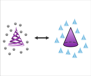
Not all fluids share this property. Depending on the symmetries obeyed by the microscopic constituents of the fluid, its stress tensor (1.2) could contain additional terms. In this article, we consider chiral fluids, or fluids that break parity or mirror symmetry at the microscopic level (figure 1a). Examples include polyatomic gases under magnetic fields (Korving et al. Reference Korving, Hulsman, Scoles, Knaap and Beenakker1967), magnetized plasma (Chapman Reference Chapman1939), fluids under rotation (Nakagawa Reference Nakagawa1956), vortex (Wiegmann & Abanov Reference Wiegmann and Abanov2014) and electron fluids (Bandurin et al. Reference Bandurin2016; Berdyugin et al. Reference Berdyugin2019), ferrofluids (Reynolds, Monteiro & Ganeshan Reference Reynolds, Monteiro and Ganeshan2023), and active and driven systems made up of spinning particles (Condiff & Dahler Reference Condiff and Dahler1964; Tsai et al. Reference Tsai, Ye, Rodriguez, Gollub and Lubensky2005; Soni et al. Reference Soni, Bililign, Magkiriadou, Sacanna, Bartolo, Shelley and Irvine2019; Hargus et al. Reference Hargus, Klymko, Epstein and Mandadapu2020; Reeves, Aranson & Vlahovska Reference Reeves, Aranson and Vlahovska2021).
Rigid body motion in a chiral fluid. (a) A fluid composed of particles driven to spin with angular velocity  $\boldsymbol {\varOmega ^{{int}}}$, for example due to an external magnetic field, is chiral. Since the microscopic constituents of the fluid break parity or mirror symmetry, the stress and viscosity tensors of the fluid no longer need be symmetric. (b) As a result, the way a rigid body moves and rotates under applied forces and torques is modified.

In these chiral systems, the stress and the viscosity tensors are no longer constrained to be symmetric,
 \begin{gather} \sigma_{ij} \neq \sigma_{ji}, \end{gather}
 \begin{gather}\eta_{ijk\ell} \neq \eta_{k\ell ij}. \end{gather}
As a result, both quantities  $\sigma ^{{h}}_{ij}$ and $\eta _{ijk\ell }$ can acquire additional contributions. The hydrostatic stress $\sigma ^{{h}}_{ij}$ can contain an antisymmetric term of the form $-\epsilon _{ijk}\chi _k$, where $\epsilon _{ijk}$ is the Levi–Civita tensor, and $\chi _k$ corresponds to an ambient torque density, which can arise, for example, in a fluid of spinning particles. Moreover, the non-zero antisymmetric part of the viscosity tensor, referred to as the odd viscosity, generates a viscous response which is non-dissipative (Avron Reference Avron1998; Lapa & Hughes Reference Lapa and Hughes2014; Ganeshan & Abanov Reference Ganeshan and Abanov2017; Markovich & Lubensky Reference Markovich and Lubensky2022; Fruchart, Scheibner & Vitelli Reference Fruchart, Scheibner and Vitelli2023).
Such a relaxation of the symmetry constraints leads to rich flow behaviour in three dimensions at low Reynolds number (Khain et al. Reference Khain, Scheibner, Fruchart and Vitelli2022). The presence of the torque density and odd viscosity alters how the chiral fluid responds to applied deformations, such as when flowing past a rigid body. Consequently, the motion of the body itself through a chiral fluid changes as well. In the overdamped regime of Stokes flow, the motion of a solid body in a fluid is described by its linear and angular velocities  $\boldsymbol {V}$ and $\boldsymbol {\varOmega }$ (Happel Reference Happel1983; Kim & Karrila Reference Kim and Karrila1991) (figure 1b). Given a reference point on the object $\boldsymbol {r_0}$, the velocity at any other point on the object is $\boldsymbol {v}(\boldsymbol {r}) = \boldsymbol {V} + \boldsymbol {\varOmega } \times (\boldsymbol {r} - \boldsymbol {r_0})$. Due to the linearity of the Stokes equations, the forces $\boldsymbol {F}$ and torques $\boldsymbol {\tau }$ on the solid body as it moves are linear functions of $\boldsymbol {V}$ and $\boldsymbol {\varOmega }$. The coefficient of proportionality is the resistance matrix $\mathbb {P}$ (also called the propulsion matrix), such that $\mathcal {F} = \mathbb {P} \mathcal {V}$, where $\mathcal {F} = [\boldsymbol {F}, \boldsymbol {\tau }]^{\rm T}$ and $\mathcal {V} = [\boldsymbol {V}, \boldsymbol {\varOmega }]^{\rm T}$. The inverse of $\mathbb {P}$, called the mobility matrix, $\mathbb {M}$, gives us the response of the solid body to external forces and torques,
 \begin{equation} \begin{bmatrix} \boldsymbol{V}\\ \boldsymbol{\varOmega} \end{bmatrix} = \mathbb{M} \begin{bmatrix} \boldsymbol{F}\\ \boldsymbol{\tau} \end{bmatrix}. \end{equation}
The external forces and torques on the solid body ( $\boldsymbol {F}, \boldsymbol {\tau }$) are balanced by the hydrodynamic forces (the forces on the solid body by the fluid), which we denote by $\boldsymbol {F}^{{fluid}}, \boldsymbol {\tau }^{{fluid}}$. In our notation, then, $\mathcal {V} = \mathbb {M} \mathcal {F} = - \mathbb {M} \mathcal {F}^{{fluid}}$.
Here and throughout most of what follows, we assume that the fluid is quiescent in the absence of the immersed object – otherwise, in (1.5), the velocity and angular velocity of the object would be with respect to the background flow of the fluid. The mobility matrix  $\mathbb {M}$ is a $6 \times 6$ matrix, which can be split into four blocks, as follows:
 \begin{equation} \mathbb{M}= \begin{bmatrix} \begin{array}{@{}c|c@{}} A & B \\ \hline T & S \end{array} \end{bmatrix}. \end{equation}
Here,  $\mathbb {M}$ depends both on the geometry of the object and the properties of the fluid, as well as the choice of reference point. In order to explain particle motion, we often turn to its geometry (Guyon et al. Reference Guyon, Hulin, Petit and Mitescu2015). In water, for example, applying a force to the centre of a sphere does not cause it to rotate; mathematically, this is captured by the fact that $T=B=0$ when the reference point is taken to be the centre of the sphere. To couple translational and rotational modes, one needs to consider more complex geometries of the solid body (Brenner Reference Brenner1965; Makino & Doi Reference Makino and Doi2003; Krapf, Witten & Keim Reference Krapf, Witten and Keim2009; Palusa et al. Reference Palusa, De Graaf, Brown and Morozov2018) or go beyond hydrodynamic interactions (Morozov et al. Reference Morozov, Mirzae, Kenneth and Leshansky2017).
Yet, the geometry of the object does not fully control its mobility: the symmetries of the fluid can play a significant role. This naturally raises the question: can we manipulate solid body motion by designing the fluid, rather than by changing the particle shape? To address this question, we must consider the symmetries of both the fluid and the solid body, and ask how these constrain the form of the mobility matrix.
In this article, we demonstrate that one can achieve complex modes of motion of simple objects by immersing them in a chiral fluid. Following the set-up in Khain et al. (Reference Khain, Scheibner, Fruchart and Vitelli2022), we consider a three-dimensional (3-D) fluid with cylindrical symmetry about the  $z$-axis and standard shear viscosity $\mu$, and focus on the effect of an odd shear viscosity denoted by $\eta ^{{o}}$. Besides its non-dissipative nature, the coefficient $\eta ^{{o}}$ is anisotropic (the $z$-axis is singled out), and parity-violating or chiral (when reflected across vertical planes, the coefficient acquires a minus sign). Each of these broken symmetries has consequences on the possible form of the mobility matrix, which we delineate in § 2. In § 3, we review different methods of computing the mobility matrix for an arbitrary solid body for a general fluid with any viscosity $\eta _{ijk\ell }$. We describe the simplest signature of a chiral fluid in § 4: a chiral particle propelling under an odd hydrostatic stress (torque). In § 5, we demonstrate the consequences of the sphere's asymmetric mobility matrix in the presence of odd viscosity, which includes the appearance of a lift force that generates spiralling trajectories. In § 6, we illustrate the rotation–translation coupling effect of $\eta ^{{o}}$ with the example of a sedimenting triangle spinning under the force of gravity. In these sections, the parity-violating and odd viscosity $\eta ^{{o}}$ produces effects that are generated by particle geometry in a standard fluid. We further emphasize the analogous roles of particle shape and fluid symmetries in § 7 by providing examples of pairs of distinct systems with similar particle motion.
2. Properties of the mobility matrix
2.1. Constraints from spatial symmetries
In a standard isotropic fluid, such as water, the mobility matrix of an object is constrained by the object's spatial symmetries. A cone, for example, is unchanged under rotations about its axis, and so its mobility matrix must remain invariant under this transformation as well. If the fluid is anisotropic, however, it is not sufficient to consider just the geometry of the object. To determine how  $\mathbb {M}$ should transform under a given coordinate transformation (such as a rotation or reflection), we must consider the effect of the transformation on both the body and the fluid. Only if the full system remains invariant – if the transformation is a symmetry of both the fluid and the object – so should $\mathbb {M}$. Here, we consider the ‘effective’ symmetry group of the fluid by looking at the symmetries obeyed by its viscosity tensor. Importantly, a cylindrically symmetric viscosity tensor is invariant under the reflection $(x, y, z) \to (x, y, -z)$, even if the constituents of the fluid are not (Khain et al. Reference Khain, Scheibner, Fruchart and Vitelli2022). Similarly, the symmetry of the mobility matrix can be higher than the symmetry of the object.
In standard isotropic fluids, only the symmetries of the object play a role, since the fluid is invariant under all rotations and reflections. In this case, it appears as if the solid body transforms ‘independently’ (Guyon et al. Reference Guyon, Hulin, Petit and Mitescu2015). An analogous example occurs for a sphere in an anisotropic fluid: here, the sphere is unchanged under all distance-preserving coordinate transformations, so we need to consider only the symmetries of the fluid.
To illustrate the complementary roles of the fluid and the solid body, let us consider a cylindrically symmetric ellipsoid (a prolate spheroid, figure 2a i), centred on the origin and oriented upright along the  $z$-axis, immersed in an isotropic fluid. Since the combined fluid and object system is invariant under rotations about the $z$-axis as well as reflections across the $x$–
$x$– $y$,
$y$,  $y$–
$y$– $z$ and $x$–
$x$– $z$ planes, the mobility matrix must be as well. To satisfy these requirements, $\mathbb {M}$ must take the form (see Appendix B)
 \begin{equation} A = \begin{bmatrix} A_{11} & & \\ & A_{11} & \\ & & A_{33} \end{bmatrix}, \quad B = 0, \quad T = 0, \quad S = \begin{bmatrix} S_{11} & & \\ & S_{11} & \\ & & S_{33} \end{bmatrix}. \end{equation}
Now, there could be other fluid/object systems with these same symmetries, and hence, with the same form of  $\mathbb {M}$; for example, a sphere immersed in an anisotropic fluid composed of aligned cylindrically symmetric ellipsoids (figure 2a ii). Even though the two solid bodies are different in these two cases, the way they move under applied forces and torques is qualitatively the same. The situation is similar in figure 2(b): the conical helix in an isotropic fluid (figure 2b i) and the cone in a fluid of conical helices (figure 2b ii) are both invariant only under cylindrical symmetry; as a result, the form of their mobility matrices must be the same. In addition to the fluid and solid body geometry, the mobility matrix depends on the choice of reference point (see Appendix A for a derivation). Throughout this section, the transformations we consider are applied about the reference point (that is, the reference point remains invariant). A proper choice of reference point is important to maximize the power of the symmetry analysis: for example, the mobility matrix of a sphere with the reference point at its centre is isotropic, while the mobility matrix of a sphere with the reference point on its surface is not.
Spatial symmetries constrain the mobility matrix. (a i) An ellipsoid in an isotropic fluid has an anisotropic mobility matrix, with different drag coefficients along and perpendicular to its long axis. (a ii) A sphere in an anisotropic fluid composed of ellipsoids has the same spatial symmetries. As a result, the two mobility matrices must have the same form. (b) A conical helix in (i) an isotropic fluid has the same spatial symmetries as a cone in (ii) a fluid composed of conical helices. As a result, the two mobility matrices must have the same form; in particular, both objects spin under applied forces. (Note that an ellipsoid in a fluid composed of conical helices would not break sufficient symmetries.) (c i) A non-chiral object, such as a cone, has zero  $B$ and $T$ blocks in an isotropic fluid. (c ii) In a parity-violating (chiral) fluid, the same cone now has $T \neq 0$, meaning that applied forces lead it to rotate.

Additionally, note that a non-zero entry in the mobility matrix that is allowed by symmetry could, in principle, be arbitrarily small for a given solid body in a fluid.
2.2. A chiral object versus a chiral fluid
In an isotropic fluid, the structure of the mobility matrix can be used to deduce the geometric properties of the solid body. For instance, the off-diagonal blocks  $B$ and $T$ are often considered signatures of the chirality of the solid body, as they couple rotation with translation (Witten & Diamant Reference Witten and Diamant2020). An object is chiral if its spatially inverted image cannot be rotated back to the original. The mobility matrix of a non-chiral object, then, can be spatially inverted and then rotated by a suitable rotation $R$ such that it remains invariant. Under these transformations, the mobility matrix transforms as
 \begin{equation} \begin{bmatrix} \begin{array}{@{}c|c@{}} A & B \\ \hline T & S \end{array} \end{bmatrix} \to \begin{bmatrix} \begin{array}{@{}c|c@{}} RAR^{{-}1} & -RBR^{{-}1} \\ \hline -RTR^{{-}1} & RSR^{{-}1} \end{array} \end{bmatrix}. \end{equation}
Requiring  $T = -RTR^{-1}$ (and the same for $B$) implies $\text {det}(T) = \text {tr}(T) = 0$, given a proper choice of reference point about which the transformations are performed. As a result, it is possible to find asymmetric non-chiral objects that have a non-zero $T$ block that cannot be removed even by moving the reference point, such as ‘taco’-like shapes with just two symmetry planes (Miara et al. Reference Miara, Vaquero-Stainer, Pihler-Puzović, Heil and Juel2024). However, sufficiently symmetric non-chiral objects do have a vanishing $T$ block. For example, a cone with a reference point along the symmetry axis has $T = 0$ (figure 2c i; see Appendix B for more details).
In an anisotropic fluid, even objects with a high degree of symmetry can exhibit chiral trajectories. In this work, we focus on a cylindrically symmetric parity-violating (or chiral) fluid that breaks mirror symmetry across planes containing the  $z$-axis, such as the one represented in figure 1(a), following the set-up in Khain et al. (Reference Khain, Scheibner, Fruchart and Vitelli2022). Let us immerse a non-chiral object in this chiral fluid – say, a cone, with its symmetry axis aligned with $z$ – and consider the most general form of the force-rotation block $T$ of its mobility matrix. If we choose the reference point along the cone's symmetry axis, the fluid/object system is invariant only under rotations about the $z$-axis, which constrains $T$ to take the form
 \begin{equation} T = \begin{bmatrix} T_{11} & T_{12} & 0\\ -T_{12} & T_{11} & 0\\ 0 & 0 & T_{33} \end{bmatrix}. \end{equation}
A quick way to check that the form of  $T$ in (2.3) is in fact invariant under rotations $R$ about the $z$-axis is to notice that the $x$–
$x$– $y$ block of $T$ is a linear combination of the identity and the Levi–Civita matrix, as is the $x$–
$x$– $y$ block of the rotation matrix $R$. Since the identity and Levi–Civita matrix each commute with themselves as well as with each other, $R$ and $T$ must commute, and so indeed $R T R^{-1} = T$.
The non-zero entries in (2.3) cannot be removed even with a different choice of reference point (see Appendix B for more details). As a consequence, the cone may spin under an applied force even if the torque is zero; in this case, a non-zero  $T$ is a signature of the chirality of the fluid, and not of the object (figure 2c ii).
2.3. Positivity
In a fluid with positive dissipative (even) viscosities, the mobility matrix  $\mathbb {M}$ is positive definite, irrespective of the presence of odd viscosities. To see this, we consider the rate of energy dissipation in a fluid,
 \begin{equation} \dot{W} = \int_{\mathcal{V}} (\partial_j v_i) \sigma_{ij} \,{\rm d}V = \int_{\mathcal{V}} (\partial_j v_i) (\eta_{ijk\ell}\partial_\ell v_k) \,{\rm d}V = \int_{\mathcal{V}} \eta_{ijk\ell}^{{e}} (\partial_j v_i) (\partial_\ell v_k) \,{\rm d}V \geqslant 0, \end{equation}
where  $\mathcal {V}$ is the fluid volume. Only the even part of the viscosity tensor contributes to $\dot {W}$ (Fruchart et al. Reference Fruchart, Scheibner and Vitelli2023); the odd viscosity does not dissipate. The rate of energy dissipation is non-negative ( $\dot {W} \geqslant 0$) provided that the even viscosities are positive (technically, this means that the tensor $\eta _{ijk\ell }^{{e}}$ acts as a positive semidefinite linear map on the space of rank two tensors (Khain et al. Reference Khain, Scheibner, Fruchart and Vitelli2022)). In an anisotropic fluid, the rates of energy dissipation along different axes may not be the same. In principle, there could exist deformation rates that do not dissipate energy. These inviscid deformations correspond to the basis vectors of the null space of $\eta ^{{e}}_{ijk\ell }$. As long as such inviscid deformations do not exist, i.e. all deformation rates correspond to a finite rate of energy dissipation, we have $\dot {W} > 0$ ( $\eta _{ijk\ell }^{{e}}$ acts as a positive definite linear map).
Now, in the case of a solid body  $S$ with surface $\partial S$ and reference point $\boldsymbol {r_0}$ immersed in an infinite volume of fluid, we can rewrite (2.4) as
 \begin{align} \dot{W} &= \int_{\mathbb{R}^3 \backslash S} (\partial_j v_i) \sigma_{ij} \, {\rm d}V = \int_{\mathbb{R}^3 \backslash S} \partial_j (v_i \sigma_{ij}) - v_i \partial_j \sigma_{ij} \,{\rm d}V = \int_{\mathbb{R}^3 \backslash S} \partial_j (v_i \sigma_{ij}) \,{\rm d}V \end{align}
 \begin{align} &= \oint_{\partial S} \boldsymbol{v}\boldsymbol{\cdot} \sigma \boldsymbol{\cdot} (-\boldsymbol{\hat{n}})\, {\rm d}A ={-}\oint_{\partial S} [\boldsymbol{V} + \boldsymbol{\varOmega} \times (\boldsymbol{r} - \boldsymbol{r_0})] \boldsymbol{\cdot} \sigma \boldsymbol{\cdot} \boldsymbol{\hat{n}}\,{\rm d}A \end{align}
 \begin{align} &={-}(\boldsymbol{V} \boldsymbol{\cdot} \boldsymbol{F}^{{fluid}} + \boldsymbol{\varOmega} \boldsymbol{\cdot} \boldsymbol{\tau}^{{fluid}}) \end{align}
 \begin{align} &=\mathcal{F}^T \mathbb{M} \mathcal{F}, \end{align}
where we have used the divergence theorem,  $\boldsymbol {\nabla }\boldsymbol {\cdot }\sigma = 0$, and $\boldsymbol {F} = -\boldsymbol {F}^{{fluid}}, \boldsymbol {\tau } = - \boldsymbol {\tau }^{fluid}$. (Note that when applying the divergence theorem, the outward normal is associated with the fluid volume, and points into the surface of the solid body.) From this, we see that if there are no inviscid deformations, $\mathcal {F}^T \mathbb {M} \mathcal {F} > 0$, and so $\mathbb {M}$ is positive-definite. In the theoretical limit of only a non-dissipative viscosity, $\dot {W} = 0$ can arise, in which case $\mathbb {M}$ is only positive semidefinite.
2.4. Symmetry
We now show that  $\mathbb {M} = \mathbb {M}^T$ if and only if there is no odd viscosity ( $\eta _{ijk\ell }^{{o}} = 0$) with the help of the Lorentz reciprocal theorem (Happel Reference Happel1983; Masoud & Stone Reference Masoud and Stone2019). In normal fluids, this theorem links two systems, where one is the ‘source’ (which produces a force), and the other is a ‘receiver’ (which measures the velocity field). The Lorentz reciprocal theorem is satisfied only in the absence of an odd viscosity (Khain et al. Reference Khain, Scheibner, Fruchart and Vitelli2022). However, generalizations can be obtained (Hosaka, Golestanian & Vilfan Reference Hosaka, Golestanian and Vilfan2023; Yuan & Olvera de la Cruz Reference Yuan and Olvera de la Cruz2023), for instance by considering two systems that have odd viscosities of opposite sign.
To see this, we introduce the following energetic inner product between the velocity field and stress tensor of two systems:
 \begin{align} \dot{W}_{1,2} &= \int_{\mathbb{R}^3 \backslash S} \partial_j v_i^{(1)} \sigma_{ij}^{(2)} \,{\rm d}V = \int_{\mathbb{R}^3 \backslash S} \partial_j v_i^{(1)} \eta_{ijk\ell}^{(2)} \partial_\ell v_k^{(2)} \,{\rm d}V \end{align}
 \begin{align} &= \int_{\mathbb{R}^3 \backslash S} \partial_j v_i^{(1)} (\eta_{ijk\ell}^{{e},(2)} + \eta_{ijk\ell}^{{o}, (2)}) \partial_\ell v_k^{(2)} \,{\rm d}V, \end{align}
where we have used the divergence theorem, the field equations  $\boldsymbol {\nabla }\boldsymbol {\cdot }\sigma = 0$ and $\boldsymbol {\nabla } \boldsymbol {\cdot } \boldsymbol {v} = 0$, and defined $\eta _{ijk\ell }^{{o}} = \frac {1}{2}(\eta _{ijk\ell } - \eta _{k\ell ij})$.
Similarly,
 \begin{align} \dot{W}_{2,1} &= \int_{\mathbb{R}^3 \backslash S} \partial_j v_i^{(2)} \sigma_{ij}^{(1)} \,{\rm d}V = \int_{\mathbb{R}^3 \backslash S} \partial_j v_i^{(2)} \eta_{ijk\ell}^{(1)} \partial_\ell v_k^{(1)} \,{\rm d}V \end{align}
 \begin{align} &= \int_{\mathbb{R}^3 \backslash S} \partial_j v_i^{(2)} (\eta_{ijk\ell}^{{e},(1)} + \eta_{ijk\ell}^{{o}, (1)}) \partial_\ell v_k^{(1)} \,{\rm d}V \end{align}
 \begin{align} &= \int_{\mathbb{R}^3 \backslash S} \partial_j v_i^{(1)} (\eta_{ijk\ell}^{{e},(1)} - \eta_{ijk\ell}^{{o}, (1)}) \partial_\ell v_k^{(2)} \,{\rm d}V, \end{align}
where we have interchanged  $ij \leftrightarrow k\ell$ for the last equality.
Then, the difference is
 \begin{equation} \dot{W}_{1,2} - \dot{W}_{2,1} = \int_{\mathbb{R}^3 \backslash S} (\eta_{ijk\ell}^{{e},(2)} - \eta_{ijk\ell}^{{e},(1)} + \eta_{ijk\ell}^{{o}, (2)} + \eta_{ijk\ell}^{{o}, (1)})\partial_j v_i^{(1)} \partial_\ell v_k^{(2)} \,{\rm d}V. \end{equation}
The Lorentz reciprocal theorem states that  $\dot {W}_{1,2} = \dot {W}_{2,1}$. From (2.14), if the two viscosities are the same ( $\eta _{ijk\ell }^{(1)} = \eta _{ijk\ell }^{(2)}$), the theorem holds only in the absence of odd viscosity. However, if the two systems have equal even viscosities and opposite odd viscosities ( $\eta _{ijk\ell }^{(1)} = \eta _{k\ell ij}^{(2)}$), such as if the external magnetic field is flipped, the theorem is satisfied.
Let us suppose that the viscosities of the two systems are equal, and choose the velocity field  $\boldsymbol {v}^{(1)}$ to correspond to the velocity of a rigid body with surface $S$. Then, as in § 2.3,
 \begin{align} \dot{W}_{1,2} &={-}\oint_{\partial S} \boldsymbol{v}^{(1)}\boldsymbol{\cdot} \sigma^{(2)} \boldsymbol{\cdot} \boldsymbol{\hat{n}}\,{\rm d}A \end{align}
 \begin{align} &={-}\oint_{\partial S} [\boldsymbol{V_1} + \boldsymbol{\varOmega_1} \times (\boldsymbol{r} - \boldsymbol{r_0})] \boldsymbol{\cdot} \sigma^{(2)} \boldsymbol{\cdot} \boldsymbol{\hat{n}}\,{\rm d}A \end{align}
 \begin{align} &= \boldsymbol{V_1} \boldsymbol{\cdot} \boldsymbol{F_2} + \boldsymbol{\varOmega_1} \boldsymbol{\cdot} \boldsymbol{\tau_2} \end{align}
 \begin{align} &=\mathcal{F}_2^T \mathbb{M} \mathcal{F}_1. \end{align}
From (2.14), in the absence of odd viscosity, we must have
 \begin{align} \mathcal{F}_2^T \mathbb{M} \mathcal{F}_1 &= \mathcal{F}_1^T \mathbb{M} \mathcal{F}_2 \end{align}
 \begin{align} &=(\mathcal{F}_2^T \mathbb{M} \mathcal{F}_1)^{\rm T}, \end{align}
which implies  $\mathbb {M} = \mathbb {M}^T$. Thus, $A = A^T, S = S^T$ and $B = T^T$ if and only if $\eta _{ijk\ell }^{{o}} = 0$.
2.5. Existence of centres
As shown in § 2.4, in the absence of odd viscosity, the mobility (and resistance) matrices must be symmetric, and so must their diagonal blocks. Meanwhile, the off diagonal blocks that couple force and angular velocity or torque and velocity are not constrained to be symmetric. In standard fluids, however, it can be shown that there exists a unique choice of reference point, called the centre of reaction or resistance, for which the torque-velocity block of the resistance matrix  $\mathbb {P}$ is symmetric (Happel Reference Happel1983; Kim & Karrila Reference Kim and Karrila1991). Similarly, the centre of twist is a choice of reference point for which block $T$ of $\mathbb {M}$ is symmetric (Krapf et al. Reference Krapf, Witten and Keim2009). Identifying these special points and working in their reference frame can be convenient for calculations; if $T$ is symmetric, it can be diagonalized by an orthonormal basis, in which the rotational motion of the rigid body can appear simpler.
Below, we show that a unique centre of twist exists as long as the fluid has no inviscid deformations, that is, all deformation rates correspond to a finite rate of energy dissipation. This condition is necessarily met in an isotropic fluid with the standard shear viscosity  $\mu$. In an anisotropic fluid, however, the dissipation rate may not be the same along all axes, in which case an inviscid deformation may exist. The existence of the centre of twist, then, is related to the properties of the even viscosities of the fluid, and does not directly depend on the presence of odd viscosities, as we will see.
From (A8), we have that under a change of reference point,
 \begin{equation} T^{\prime} = T^0 + S [\![{\times} \boldsymbol{R}]\!], \end{equation}
or, in index notation,
 \begin{equation} T^{\prime}_{ij} = T^0_{ij} + \epsilon_{\ell kj}R_k S_{i\ell}, \end{equation}
where  $T^{\prime }$ is computed with respect to $\boldsymbol {r_0^{\prime }}$ and $T^0$ is computed with respect to $\boldsymbol {r_0}$. Here, we have defined $[\![ \boldsymbol {R} \times ]\!]_{ik} = [\![\times \boldsymbol {R}]\!]_{ik} = \epsilon _{ijk} R_j$ such that $[\![ \boldsymbol {R} \times ]\!] \boldsymbol {v} = \boldsymbol {R} \times \boldsymbol {v}$ and $\boldsymbol {v} [\![\times \boldsymbol {R}]\!] = \boldsymbol {v} \times \boldsymbol {R}$ for any vector $\boldsymbol {v}$, and $\boldsymbol {R} = \boldsymbol {r_0}^{\prime } - \boldsymbol {r_0}$. Now, the antisymmetric part of $T^{\prime }$ is zero when
 \begin{align} T_{ij}^0 - T_{ji}^0 &={-}(\epsilon_{\ell kj} R_k S_{i \ell} - \epsilon_{\ell ki}R_k S_{j\ell}) \end{align}
 \begin{align} &= \epsilon_{jk\ell} R_k S_{i\ell} - \epsilon_{ik\ell}R_k S_{j\ell}. \end{align}
Applying  $\epsilon _{mij}$ to both sides and using the identities
 \begin{gather} \epsilon_{mij}\epsilon_{jk\ell} = \epsilon_{jmi}\epsilon_{jk\ell} = \delta_{mk}\delta_{i\ell} - \delta_{m\ell}\delta_{ik}, \end{gather}
 \begin{gather}\epsilon_{mij}\epsilon_{ik\ell} = \epsilon_{ijm}\epsilon_{ik\ell} = \delta_{jk}\delta_{m\ell} - \delta_{j\ell}\delta_{mk}, \end{gather}
we have
 \begin{align} \epsilon_{mij}(T_{ij}^0 - T_{ji}^0) &= R_{m}S_{ii} - R_{i}S_{im} - R_{j}S_{jm} + R_{m}S_{jj} \end{align}
 \begin{align} &= 2(R_m S_{ii} - R_i S_{im}) \end{align}
 \begin{align} &= 2[\boldsymbol{R}\boldsymbol{\cdot}(\text{tr}(S)\mathbb{I} - S)]_m. \end{align}
The centre of twist exists if the equation above has a solution for some  $\boldsymbol {R}$. Whether this is the case depends on the properties of the matrix $\text {tr}(S)\mathbb {I} - S$.
In the absence of odd viscosity and any inviscid deformations, the block  $S$ is symmetric and positive-definite, and can thus be diagonalized, in which case its three positive eigenvalues, $S_1, S_2, S_3$, are along the diagonal. In this basis,
 \begin{equation} \text{tr}(S)\mathbb{I} - S = \begin{bmatrix} S_2 + S_3 & 0 & 0\\ 0 & S_1 + S_3 & 0 \\ 0 & 0 & S_1 + S_2 \end{bmatrix}. \end{equation}
The determinant of this matrix is always positive, and so  $\text {tr}(S)\mathbb {I} - S$ is invertible. As a result, there is a unique solution for $\boldsymbol {R}$, and a unique centre of twist.
The presence of odd viscosity does not affect the properties of  $\text {tr}(S)\mathbb {I} - S$, assuming that there are no inviscid deformations (i.e. enough even viscosities are non-zero). Then, even though $S$ is not symmetric, it is not antisymmetric, and must be positive-definite. As a result, the eigenvalues of $S$ must have a positive real part. Whether or not $S$ is diagonalizable or has a Jordan block of size $2$ or $3$, the diagonal entries of $\text {tr}(S)\mathbb {I} - S$ must be positive, and thus $\text {det}(\text {tr}(S)\mathbb {I} - S) > 0$. Hence, a unique centre of twist exists.
3. Computing the mobility matrix
In § 2, we constrained the form of the mobility matrix based on symmetry considerations. Given a viscosity tensor  $\eta _{ijk\ell }$, we would now like to explicitly obtain $\mathbb {M}$ for a desired shape. To that end, we outline a few methods of solving for the mobility matrix, beginning with the classic boundary value problem approach.
3.1. Boundary value problem
In this method, we first solve the resistance (also called propulsion) problem (Kim & Karrila Reference Kim and Karrila1991), and derive the mobility through matrix inversion. For clarity, let us name the blocks of the resistance matrix,
 \begin{equation} \mathbb{P} = \begin{bmatrix} \begin{array}{@{}c|c@{}} P_1 & P_2 \\ \hline P_3 & P_4 \end{array} \end{bmatrix}. \end{equation}
 Suppose we have a solid body moving through a fluid with constant velocity  $\boldsymbol {V}$. To compute the velocity field outside the body, we move to a frame in which the body is held stationary, and thus $\boldsymbol {v}(r \to \infty ) = -\boldsymbol {V}$. We solve the Stokes equations in (1.1) subject to incompressibility and the additional no-slip boundary condition on the surface $\partial S$ of the solid body, $\boldsymbol {v}(r \in \partial S) = 0$. Note that other boundary conditions could be appropriate, depending on the particular realization of an odd viscous fluid and the microscopic interactions between the boundary and the fluid constituents.
With  $\boldsymbol {v}$ and $P$ in hand, we compute the stress in the fluid using (1.2). Then, the force and torque on the solid body from the fluid are given by integrals over the object surface,
 \begin{gather} \boldsymbol{F}^{{fluid}} = \oint \sigma \boldsymbol{\cdot} \hat{\boldsymbol{n}}\,{\rm d}A, \end{gather}
 \begin{gather}\boldsymbol{\tau}^{{fluid}} = \oint (\boldsymbol{r} - \boldsymbol{r_0}) \times \sigma \boldsymbol{\cdot} \hat{\boldsymbol{n}}\,{\rm d}A, \end{gather}
where  $\boldsymbol {r_0}$ is a reference point and $\hat {\boldsymbol {n}}$ is the outward normal. Through the integrals above, we acquire the coefficients of proportionality between the force and torque and the velocity of the solid body, i.e. blocks $P_1$ and $P_3$ of the resistance matrix.
The blocks  $P_2$ and $P_4$ are computed similarly. For this case, we suppose the solid body spins with angular velocity $\boldsymbol {\varOmega }$. Solving the boundary value problem, computing the stress, and integrating over the object surface provides the forces and torques, which yields the remaining blocks. Once the full resistance matrix is computed, we invert to obtain the mobility matrix.
In general, solving the Stokes equation analytically is feasible for shapes with a high degree of symmetry, such as the sphere. For other geometries, a common approach is to numerically solve for the velocity field outside the object using finite element methods or other approaches. In this work, we solve the boundary value problem analytically for the sphere in § 5 in order to compute block  $A$ of $\mathbb {M}$. In general, to compute this block, it is necessary to solve for the full resistance matrix as outlined above, since $A = (P_1 - P_2 P_4^{-1} P_3)^{-1}$. For a sphere in an odd viscous fluid, however, we find that $P_3 = 0$ (see § 5), and so we simply have $A = P_1^{-1}$ and the rotational half of the problem is not needed.
3.2. Boundary integral method
Rather than solving for the velocity field in the bulk fluid outside of the solid body as in § 3.1, the boundary integral method (also called the single-layer potential) reformulates the Stokes equations into integral form over the object's surface (Kim & Karrila Reference Kim and Karrila1991; Guazzelli & Morris Reference Guazzelli and Morris2009). Conceptually, the boundary condition at the surface of the object can be thought to exert forces on the fluid (or vice versa), which bend the fluid flow around the solid body. By building the object out of force singularities which are distributed on its surface, we can mimic the boundary condition and solve the mobility problem directly.
First, we obtain the velocity field due to a point force  $\boldsymbol {f}(\boldsymbol {r}) = \boldsymbol {f} \delta ^3(\boldsymbol {r})$ by solving the Stokes equation (1.1),
 \begin{equation} \boldsymbol{v}(\boldsymbol{r}) = \mathbb{G}(\boldsymbol{r}) \boldsymbol{f}, \end{equation}
where  $\boldsymbol {v}$ is termed the Stokeslet, and $\mathbb {G}$ is the Green's function or Oseen tensor (for a description of the solution method for an arbitrary viscosity tensor, see Khain et al. (Reference Khain, Scheibner, Fruchart and Vitelli2022)).
In a fluid with shear viscosity  $\mu$, the Green's function is given by
 \begin{equation} \mathbb{G}^{(0)}_{ij}(\boldsymbol{r}) = \frac{1}{8{\rm \pi}\mu r^3}(\delta_{ij} r^2 + r_i r_j). \end{equation}
For the case of a rigid body, the external velocity field can then be expressed as
 \begin{equation} v_i(\boldsymbol{r}) = \oint \mathbb{G}_{ij}(\boldsymbol{r'} - \boldsymbol{r})f_j(\boldsymbol{r'})\,{\rm d}A(\boldsymbol{r'}), \end{equation}
where the integral is over the object's surface (Burgers Reference Burgers1938; Yamakawa Reference Yamakawa1970; Pozrikidis Reference Pozrikidis1992) and
 \begin{equation} F_j = \oint f_j(\boldsymbol{r'}) \,{\rm d}A(\boldsymbol{r'}) \end{equation}
is the external force on the sphere, or equivalently, the force the sphere exerts on the fluid.
In the case of the sphere, the force distribution  $f_j$ can be guessed: due to the sphere's symmetry, the force distribution must be uniform, so $f_j(\boldsymbol {r'}) = F_j / 4{\rm \pi} a^2$. The velocity field at $\boldsymbol {r} = 0$ (the centre of the sphere) is the rigid body velocity of the sphere, $\boldsymbol {V}$, which we are looking for. Then,
 \begin{equation} V_i = v_i(0) = \frac{F_j}{4{\rm \pi} a^2}\oint \mathbb{G}_{ij}(\boldsymbol{r'})\,{\rm d}A(\boldsymbol{r'}). \end{equation}
From this, we read off the mobility matrix block  $A$ to be
 \begin{equation} A_{ij} = \frac{1}{4{\rm \pi} a^2}\oint \mathbb{G}_{ij}(\boldsymbol{r'})\,{\rm d}A(\boldsymbol{r'}). \end{equation}
Computing the mobility matrix with this method requires calculating the Green's function  $\mathbb {G}$ in real space, as done in Yuan & Olvera de la Cruz (Reference Yuan and Olvera de la Cruz2023).
An alternative approach is to carry out the integration over the sphere surface in Fourier space, which avoids the extra residue integration required to compute  $\mathbb {G}$ in real space. In Fourier space, the velocity field due to a force distribution $\boldsymbol {f}$ is given by
 \begin{equation} v_i(\boldsymbol{q}) = G_{ij}(\boldsymbol{q}) f_j(\boldsymbol{q}). \end{equation}
But then,
 \begin{equation} v_i(\boldsymbol{r}) = \frac{1}{(2{\rm \pi})^3}\int G_{ij}(\boldsymbol{q}) f_j(\boldsymbol{q}) {\rm e}^{{\rm i}\boldsymbol{q}\boldsymbol{\cdot}\boldsymbol{r}} \,{\rm d}^3 \boldsymbol{q}. \end{equation}
In this case, constraining the force singularities to lie on the surface of the sphere amounts to choosing
 \begin{equation} f_j(\boldsymbol{r}) = f(r) \boldsymbol{e}_j = \frac{F_j}{4{\rm \pi} a^2}\delta(r - a). \end{equation}
In Fourier space, the force is
 \begin{equation} f_j(\boldsymbol{q}) = F_j \frac{\sin{(qa)}}{qa}. \end{equation}
Inserting this expression into (3.11) and evaluating at  $r = 0$ as before yields
 \begin{equation} A_{ij} = \frac{1}{(2{\rm \pi})^3}\int G_{ij}(\boldsymbol{q}) \frac{\sin{(qa)}}{qa} \,{\rm d}^3\boldsymbol{q}. \end{equation}
Obtaining the mobility matrix in this way is referred to as the shell localization method in Levine & Lubensky (Reference Levine and Lubensky2001) and Lier et al. (Reference Lier, Duclut, Bo, Armas, Jülicher and Surówka2023). Note that this method works only for a sphere under a force; if there is also a torque applied, it may not be sufficient to just consider the Stokeslets to compute the rigid body velocity.
3.3. Discrete Stokeslet method
In §§ 3.1–3.2, we reviewed two methods for computing the mobility matrix that can be solved analytically in the case of a sphere. For rigid bodies with fewer degrees of symmetry, however, analytically solving the boundary value problem in § 3.1 is generally intractable. Meanwhile, although the boundary integral formulation of (3.6) applies to asymmetric shapes, the force singularity distribution may no longer be uniform and is in general unknown. To overcome this problem, we describe a discrete variation of the singularity method of § 3.2 in which the forces can be solved for given a choice for the positions of the Stokeslets (or in this case, small spheres). This method bears similarity to the immersed boundary method, in which the boundary conditions at the surface of an object are modelled through a forcing function (Mittal & Iaccarino Reference Mittal and Iaccarino2005; Verzicco Reference Verzicco2023). In our case, to determine the force magnitude and direction associated with each Stokeslet, we follow the formalism originally developed for modelling polymer chains in Kirkwood & Riseman (Reference Kirkwood and Riseman1948), Bloomfield, Dalton & Van Holde (Reference Bloomfield, Dalton and Van Holde1967), Rotne & Prager (Reference Rotne and Prager1969), Yamakawa (Reference Yamakawa1970) and Meakin & Deutch (Reference Meakin and Deutch1987), more recently used for general rigid bodies and reviewed in Krapf et al. (Reference Krapf, Witten and Keim2009), Mowitz & Witten (Reference Mowitz and Witten2017) and Witten & Diamant (Reference Witten and Diamant2020) and reproduce the method below. Our code implementing this method is available at https://doi.org/10.5281/zenodo.12556863.
As before, the goal is to compute the velocity of a rigid body moving in a fluid under an external force  $\boldsymbol {F}$. We begin by covering the object with a distribution of small spheres of radius $a$. Assuming that the distance between the spheres is significantly larger than their size, we can neglect the near-field velocity field generated by the spheres, and treat each one as a Stokeslet under a yet undetermined force $\boldsymbol {f^{\alpha }}$. Given a distribution of $N$ Stokeslets, the velocity field at the position of Stokeslet $\alpha$ is given by a linear superposition of velocity fields generated by the remaining Stokeslets,
 \begin{equation} \boldsymbol{v}^{\alpha}(\boldsymbol{r}^{\alpha}) = \mathbb{G}(\boldsymbol{r}^{\alpha}-\boldsymbol{r}^{\beta})\boldsymbol{f}^{\beta}, \end{equation}
where  $\mathbb {G}$ is the Green's function and $\boldsymbol {f}$ is the applied force (note the summation over $\beta$). If these were free Stokeslets, we would simply impose that Stokeslet $\alpha$ move with velocity $\boldsymbol {v}^\alpha$. However, since these Stokeslets model a rigid body, and are thus rigidly connected, Stokeslet $\alpha$ moves instead with velocity
 \begin{equation} \boldsymbol{u}^{\alpha}(\boldsymbol{r}^\alpha) = \boldsymbol{V}(\boldsymbol{r_0}) + \boldsymbol{\varOmega} \times (\boldsymbol{r}^{\alpha}-\boldsymbol{r_0}) , \end{equation}
where  $\boldsymbol {V}$ and $\boldsymbol {\varOmega }$ are the velocity and angular velocity of the rigid body, respectively, and $\boldsymbol {r_0}$ is a reference point on the object.
Due to the mismatch of the velocities of the Stokeslet and the fluid around it, the Stokeslet exerts a force on the fluid given by
 \begin{equation} \boldsymbol{f}^\alpha = P_1 (\boldsymbol{u}^\alpha - \boldsymbol{v}^\alpha), \end{equation}
where  $P_1$ is the top left-hand block of the resistance matrix of a small sphere with radius $a$. In the case we consider below, we find that $P_3 = 0$, so we can substitute $P_1 = A^{-1}$. In a standard fluid with shear viscosity $\mu$, the coefficient in (3.17) is simply Stokes drag. This block of the mobility/resistance matrix of the sphere must be computed separately in order to apply this method, for example by using one of the techniques in §§ 3.1 or 3.2.
Combining the previous three equations, we can write the velocity of Stokeslet  $\alpha$ as
 \begin{align} \boldsymbol{u}^\alpha(\boldsymbol{r}^\alpha) &= \boldsymbol{V}(\boldsymbol{r_0}) + \boldsymbol{\varOmega} \times (\boldsymbol{r}^{\alpha}-\boldsymbol{r_0}) \end{align}
 \begin{align} &= \mathbb{G}(\boldsymbol{r}^{\alpha}-\boldsymbol{r}^{\beta})\boldsymbol{f}^{\beta} + \delta^{\alpha \beta} A \boldsymbol{f}^\beta. \end{align}
Meanwhile, the external force and torque on the rigid body are given by
 \begin{gather} \boldsymbol{F} = \sum_{\alpha}\boldsymbol{f}^{\alpha}, \end{gather}
 \begin{gather}\boldsymbol{\tau} = \sum_{\alpha} (\boldsymbol{r}^{\alpha} - \boldsymbol{r}_0) \times \boldsymbol{f}^{\alpha}. \end{gather}
 Since (3.19) is linear in the  $\boldsymbol {f}$s, we can solve for $\boldsymbol {F}$ and $\boldsymbol {\tau }$ in terms of $\boldsymbol {V}$ and $\boldsymbol {\varOmega }$. Introducing a helper $3N \times 6$ matrix $U$,
$U$,
 \begin{equation} U = \begin{pmatrix} U^1 \\ U^2 \\ \vdots \\ U^N \end{pmatrix} \end{equation}
with blocks
 \begin{equation} U^{\alpha} = \begin{bmatrix} 1 & 0 & 0 & 0 & (z^\alpha - z_0) & -(y^\alpha - y_0)\\ 0 & 1 & 0 & -(z^\alpha - z_0) & 0 & (x^\alpha - x_0)\\ 0 & 0 & 1 & (y^\alpha - y_0) & -(x^\alpha - x_0) & 0\\ \end{bmatrix} \end{equation}
we can write  $\boldsymbol {u} = U \mathcal {V}$ and $\mathcal {F} = U^T \boldsymbol {f}$. But then (3.19) takes the form
 \begin{equation} \mathbb{G}_{{full}}\, \boldsymbol{f} = U \mathcal{V}, \end{equation}
where  $\mathbb {G}_{{full}}$ is a $3N \times 3N$ matrix composed of $3 \times 3$ blocks. If $\alpha = \beta$, the block is simply $A$, and if $\alpha \neq \beta$, the block is given by $\mathbb {G}(\boldsymbol {r}^\alpha -\boldsymbol {r}^\beta )$. From this, it follows that
 \begin{equation} \mathcal{F} = U^T \mathbb{G}_{{full}}^{{-}1} U \mathcal{V} \end{equation}
and thus the mobility matrix for the rigid body is
 \begin{equation} \mathbb{M} = (U^T \mathbb{G}_{{full}}^{{-}1} U)^{{-}1}. \end{equation}
 Using (3.26) and (1.5), we compute the rigid body  $\boldsymbol {V}$ and $\boldsymbol {\varOmega }$. Finally, to obtain the new positions of the Stokeslets, we use (3.16) and integrate the overdamped equation
 \begin{equation} \dot{\boldsymbol{r}^\alpha} = \boldsymbol{u}^\alpha. \end{equation}
 To demonstrate the validity of this method, we consider the case of a rigid sphere, first in a standard fluid with shear viscosity  $\mu$. By uniformly covering a spherical shell with Stokeslets (figure 3a) using a Fibonacci lattice (González Reference González2010), one can both recover the velocity field outside the sphere (figure 3b, red) as well as the mobility matrix (figure 3c, red) in the large $N$ limit. In the sections that follow, we use the methods described in §§ 3–3.3 to illustrate the effects of a chiral fluid on particle motion, and confirm their validity in the presence of odd viscosity.
Comparison between theory and the Stokeslet method for modelling a rigid sphere with odd viscosity. (a) The sphere is built out of  $N$ Stokeslets uniformly distributed on its surface. (b) The flow field outside the sphere for $N=1000$ Stokeslets (i) without and (ii) with odd viscosity $\eta ^{{o}}$. By covering the sphere with ‘odd’ Stokeslets (Stokeslets computed in the presence of a non-zero odd viscosity), one can successfully model a rigid sphere in an odd viscous flow as done for the standard fluid. (c) The mobility matrix entries for the sphere as a function of $N$. The off-diagonal terms (in blue) are non-zero only in the presence of $\eta ^{{o}}$. As $N$ increases, the drag coefficients converge to the theoretical values (dashed lines), even in the case of odd viscosity. For these computations, $R = 1, a = 0.001, \eta ^o/\mu = 0.1$.

4. Propulsion with odd hydrostatic stress
Chiral fluids are typically made of particles that all rotate in the same way. As a consequence, their hydrostatic stress,
 \begin{equation} \sigma^{{h}}_{i j} ={-} p \delta_{i j} -\epsilon_{ijk} \chi_k, \end{equation}
typically contains an antisymmetric part  $-\epsilon _{ijk}\chi _k$ capturing local torques in addition to the pressure. As these torques are present even in the unperturbed fluid, they usually are responsible for the most visible effects of the chirality. We now demonstrate that a chiral object put in a chiral fluid can propel by converting the local torques into linear motion.
This can be understood as follows. We assume that  $\chi _k$ is constant in time and uniform in space (Banerjee et al. Reference Banerjee, Souslov, Abanov and Vitelli2017; Han et al. Reference Han, Fruchart, Scheibner, Vaikuntanathan, De Pablo and Vitelli2021; Markovich & Lubensky Reference Markovich and Lubensky2021). In this case, the torque density induces a net torque $\tau _k = 2\chi _k V$ on a solid body of volume $V$ immersed in the fluid. Therefore, we expect that the object will rotate; this is indeed what happens, and this effect is described by the block $S$ in the mobility matrix. In addition, when the block $B$ is non-zero, the presence of a net torque also leads to linear motion.
In a fluid with cylindrical symmetry, such as in a fluid composed of particles spinning with  $\boldsymbol {\varOmega ^{{int}}} = \varOmega ^{{int}}\hat {\boldsymbol {z}}$ or under an external magnetic field in the $z$-direction, the allowed form of the hydrostatic stress is $\chi _k = \chi _z$ (Khain et al. Reference Khain, Scheibner, Fruchart and Vitelli2022). To evaluate the response of the body to this driving torque, we apply the mobility matrix formalism in (1.5). In the absence of forces, the translational velocity of the rigid object is $\boldsymbol {V} = B \boldsymbol {\tau }$, which simplifies to
 \begin{equation} V_i = 2V B_{iz} \chi_z. \end{equation}
Similarly, the body's rotational velocity is  $\varOmega _i = 2 V S_{iz} \chi _z$.
Consequently, any solid body with a non-zero  $B$ – such as an object with translational–rotational coupling – spontaneously propels in a chiral fluid. Figure 4 demonstrates the trajectory of a triple helix in a fluid with an ambient torque density. To model the helix, we cover it with a chain of Stokeslets as in § 3.3, where the Green's function is given by (3.5).
A triple helix propelled in a fluid with torque density. (a) If the axis of the helix is aligned with the torque direction, the helix rotates about and moves along this axis. The velocity of propulsion is linear in  $\tau$, as evident from (4.5). (b) If the torque and helix axis are orthogonal to each other, the helix still experiences propulsion along the torque direction, although it is weaker and with an opposite sign. In both cases, the chirality of the helix (red versus blue curves) flips the sign of the velocity response.

Each strand of the triple helix is given by the equation
 \begin{gather} x = r \cos{(k z + \phi_0)}, \end{gather}
 \begin{gather}y = r \sin{(k z + \phi_0)}, \end{gather}
with  $z \in [0, 2{\rm \pi} ), r = 1/2, k = 2$. The strands are rotated by $120^{\circ }$ with respect to each other by taking $\phi _0 = 0, 2{\rm \pi} /3, 4{\rm \pi} /3$. Each strand consists of $100$ Stokeslets of radius $a = 0.01$,

The mobility matrix for the helix is shown in pictorial form in (
4.5). The colours represent the qualitative ordering of the entries, and are chosen to highlight the structure of the mobility matrix. Red (blue) squares are positive (negative) entries, and white squares are zero (for a numerical version, see (C1) in Appendix C). Due to non-zero entries in block  $B$, the helix propels in the direction of an applied torque in addition to rotating, as shown in figure 4.
The propulsion of the helix is similar to the mechanism many bacteria use to swim, which involves rotating their helical flagella (Lauga Reference Lauga2016). Here, however, the helix is driven externally by the torques in the fluid.
5. Spiralling with a lift force
In § 4, the only role of the broken chirality in the fluid was to produce a net torque on the object through the antisymmetric part of the hydrostatic stress; for example, an immersed sphere in such a fluid would spin with constant speed (Khain et al. Reference Khain, Scheibner, Fruchart and Vitelli2022). In addition to an asymmetric stress, a chiral fluid may also have an asymmetric viscosity tensor. As shown in § 2.4, in the presence of an odd viscosity  $\eta _{ijk\ell }^{{o}}$, the mobility matrix can also have an antisymmetric part.
To illustrate the effect of odd viscosity and an asymmetric  $\mathbb {M}$ on the motion of an immersed body, we consider the odd shear viscosities $\eta _1^{{o}}$ and $\eta _2^{{o}}$ that emerge in a 3-D fluid with cylindrical symmetry (Khain et al. Reference Khain, Scheibner, Fruchart and Vitelli2022), and simplify to the limit $\eta ^{{o}} \equiv \eta _2^{{o}} = -\eta _1^{{o}}/2$. The viscosity coefficient $\eta ^{{o}}$ used here corresponds to the viscosity $-{\boldsymbol {\ell }}/{4}$ in (10) of Markovich & Lubensky (Reference Markovich and Lubensky2021) in the limit where $\boldsymbol {\ell } = \ell _z \hat {\boldsymbol {z}}$, $-\mu _o$ in Yuan & Olvera de la Cruz (Reference Yuan and Olvera de la Cruz2023), and $-{\eta ^{{o}}}/{2}$ in Hosaka et al. (Reference Hosaka, Golestanian and Vilfan2023). In the presence of this odd viscosity, the Stokes equation takes the form
 \begin{equation} 0 ={-}\boldsymbol{\nabla}\tilde{P} + \begin{bmatrix} \mu & -\eta^{{o}} & 0 \\ \eta^{{o}} & \mu & 0 \\ 0 & 0 & \mu \end{bmatrix} \Delta \boldsymbol{v} , \end{equation}
where  $\tilde P = P + \eta ^{{o}} (\partial _x v_y - \partial _y v_x)$.
To model the solid body with the Stokeslet method (§ 3.3), we must include the effect of the odd viscosity on the velocity field. In the limit of a small odd viscosity ( $\varepsilon \equiv \eta ^{{o}}/\mu \ll 1$), the perturbative correction to the Green's function is
 \begin{equation} \mathbb{G}^{(1)} = \frac{1}{8 {\rm \pi}\mu r^3} \begin{bmatrix} 0 & x^2 + y^2 & yz\\ -(x^2 + y^2) & 0 & -xz\\ -yz & xz & 0 \end{bmatrix}. \end{equation}
 The ‘odd’ Stokeslet  $\mathbb {G} = \mathbb {G}^{(0)} + \varepsilon \mathbb {G}^{(1)}$ has a more complex flow field than the standard point force solution. For example, under a constant force $F_z$ in the $z$-direction, the correction to the Stokeslet velocity field due to the odd viscosity is an azimuthal flow: $\boldsymbol {v} = \mathbb {G} F_z\boldsymbol {\hat {z}} = (\varepsilon F_z/8 {\rm \pi}\mu ) r^{-3} (yz \boldsymbol {\hat {x}} - xz \boldsymbol {\hat {y}}) = (\varepsilon F_z/8 {\rm \pi}\mu ) r^{-2} z \boldsymbol {\hat {\phi }}$ (Khain et al. Reference Khain, Scheibner, Fruchart and Vitelli2022).
For a sphere in a standard fluid, block  $A$ of the mobility matrix (top left-hand block) is purely diagonal, giving us the familiar Stokes drag law
 \begin{equation} \boldsymbol{V} = \frac{1}{6{\rm \pi} \mu a} \boldsymbol{F}. \end{equation}
 To generalize this expression for a fluid with odd viscosity, we must compute the mobility matrix of the sphere using the methods in §§ 3.1 or 3.2. We begin with solving the boundary value problem (5.1) by expanding  $\boldsymbol {v} = \boldsymbol {v_0} + \varepsilon \boldsymbol {v_1}, P = P_0 + \varepsilon P_1$ (for a non-perturbative approach, see Everts & Cichocki (Reference Everts and Cichocki2024)). In previous work (Khain et al. Reference Khain, Scheibner, Fruchart and Vitelli2022), we found that for flow in the $z$-direction, the force on the sphere is not modified to first order in $\varepsilon$. Here, we return to this problem, and compute the velocity field for the case in which the axis of the odd viscosity (taken to be $\boldsymbol {\hat {z}}$) is perpendicular to the flow. Solutions for a general $\boldsymbol {V}$ are presented below and agree with Hosaka et al. (Reference Hosaka, Golestanian and Vilfan2023) (the viscosity coefficient $\eta ^{o}$ used here corresponds to the viscosity $-{\eta ^{{o}}}/{2}$ in Hosaka et al. (Reference Hosaka, Golestanian and Vilfan2023)).
The known zeroth-order flow past a sphere is (Kim & Karrila Reference Kim and Karrila1991)
 \begin{gather} \boldsymbol{v_0}(\boldsymbol{r}) ={-}\boldsymbol{V} + 6{\rm \pi} \mu a\left(1 + \frac{a^2}{6} \varDelta \right) \mathbb{G}^{(\mathbb{0})}\boldsymbol{\cdot} \boldsymbol{V}, \end{gather}
 \begin{gather}P_0 (\boldsymbol{r}) = \frac{3a\mu}{2r^3}(\boldsymbol{V}\boldsymbol{\cdot} \boldsymbol{r}). \end{gather}
The first-order solution in  $\varepsilon$ is a linear combination of the Green's function and its Laplacian,
 \begin{gather} \boldsymbol{v_1}(\boldsymbol{r}) = 6{\rm \pi} \mu a\left(1 + \frac{a^2}{6} \varDelta \right) \mathbb{G}^{(0)} \boldsymbol{\cdot} \left(\boldsymbol{\hat{z}} \times \frac{\boldsymbol{V}}{2} \right) + 6{\rm \pi} \mu a \left(1 + \frac{a^2}{6} \varDelta \right)\mathbb{G}^{(1)} \boldsymbol{\cdot} \boldsymbol{V}, \end{gather}
 \begin{gather}P_1({\boldsymbol{r}}) ={-}\frac{9a\mu}{4r^3}(\boldsymbol{z}\times \boldsymbol{V}). \end{gather}
To obtain the forces on the sphere due to the fluid, we compute the stress and integrate over the surface of the sphere as in (3.2). For  $\boldsymbol {V} = V_x \boldsymbol {\hat {x}}$, this results in the expected Stokes drag, $F_x^{{fluid}} = -6{\rm \pi} \mu a V_x$, at zeroth order. In the presence of odd viscosity, the stress contains three contributions,
 \begin{equation} \sigma_{ij} ={-}P \delta_{ij} + \mu (\partial_i v_j + \partial_j v_i) + \sigma^{\eta^{{o}}}_{ij}, \end{equation}
where
 \begin{equation} \sigma^{\eta^{{o}}} = \eta^{{o}} \begin{bmatrix} -2(\partial_x v_y + \partial_y v_x) & 2(\partial_x v_x - \partial_y v_y) & -\partial_y v_z - \partial_z v_y \\ 2(\partial_x v_x - \partial_y v_y) & 2(\partial_x v_y + \partial_y v_x) & \partial_x v_z + \partial_z v_x\\ -\partial_y v_z - \partial_z v_y & \partial_x v_z + \partial_z v_x & 0 \end{bmatrix}. \end{equation}
Notice, then, the contributions to the stress at first order in  $\varepsilon$: $P_1$ contributes to the first term; $\boldsymbol {v_1}$ contributes to the second; $\boldsymbol {v_0}$ contributes to the third. Carrying out the integral in (3.2) results in a first-order correction to the force on the sphere. This correction, however, is not in the direction of the uniform flow, but perpendicular to it,
 \begin{equation} F_y^{{fluid}} ={-}3{\rm \pi} \varepsilon \mu a V_x = \frac{\varepsilon}{2}F_x^{{fluid}}. \end{equation}
Permuting indices, we see that a uniform flow in the  $y$-direction gives a force in the $-x$-direction. Rewriting in terms of the external forces on the sphere, the top left-hand block of the resistance matrix for the sphere takes the form
 \begin{equation} \begin{bmatrix} F_x \\ F_y \\ F_z \end{bmatrix} = 6{\rm \pi} \mu a \begin{bmatrix} 1 & -\varepsilon/2 & 0\\ \varepsilon/2 & 1 & 0\\ 0 & 0 & 1 \end{bmatrix} \begin{bmatrix} V_x\\ V_y\\ V_z \end{bmatrix}, \end{equation}
which recovers the result in Hosaka et al. (Reference Hosaka, Golestanian and Vilfan2023). To compute the top left-hand block of mobility matrix, we invert the above equation, only keeping terms of  $O(\varepsilon )$, to find
 \begin{equation} \begin{bmatrix} V_x \\ V_y \\ V_z \end{bmatrix} = \frac{1}{6{\rm \pi} \mu a} \begin{bmatrix} 1 & \varepsilon/2 & 0\\ -\varepsilon/2 & 1 & 0\\ 0 & 0 & 1 \end{bmatrix} \begin{bmatrix} F_x\\ F_y\\ F_z \end{bmatrix} . \end{equation}
Alternatively, we can obtain the same result by integrating the Green's function as in § 3.2, as done in Yuan & Olvera de la Cruz (Reference Yuan and Olvera de la Cruz2023) (the viscosity coefficient  $\eta ^{o}$ used here corresponds to the viscosity $-\mu _{o}$ in Yuan & Olvera de la Cruz (Reference Yuan and Olvera de la Cruz2023)). Notice that the mobility matrix is indeed asymmetric, even to first order in the odd viscosity. In Appendix B, we further show by symmetry arguments that a cylindrically symmetric viscosity can lead to a lift force for the sphere only if it is both parity-violating and non-dissipative.
We can now check if the method described in § 3.3 works in the presence of odd viscosity. To model a sphere in an odd viscous fluid, we must build it out of the modified Stokeslet in (5.2), and include the modified  $A$ in (3.17). In figure 3(b ii), we demonstrate excellent agreement of the numerical and analytical velocity fields outside of the sphere. Moreover, in figure 3(c), we find that the odd mobility matrix entries (in blue) computed with the Stokeslet method converge to the theoretical values at large $N$. The dashed theory lines for $\mathbb {M}_{12}$ and $\mathbb {M}_{21}$ come from (5.12), while $\mathbb {M}_{45}$ and $\mathbb {M}_{54}$ (in block $S$) are taken from Yuan & Olvera de la Cruz (Reference Yuan and Olvera de la Cruz2023). A pictorial representation of the full mobility matrix is as follows:

Let us now examine the consequences of the antisymmetric part of the mobility matrix of the sphere. Suppose we immerse a spherical colloidal particle in an odd viscous fluid and place it under optical tweezers (figure 5a), such that it is in a planar radial potential  $\boldsymbol {F} = -k(x,y,0)$. Here, we are not interested in the $z$-motion of the sphere. If the odd viscosity axis is in the $z$-direction, we can write down the equations of motion using the mobility matrix above,
 \begin{gather} \dot{x} ={-}k \gamma \left(x + \frac{\varepsilon}{2}y\right), \end{gather}
 \begin{gather}\dot{y} ={-}k \gamma \left(-\frac{\varepsilon}{2}x + y\right), \end{gather}
 \begin{gather}\dot{z} = 0, \end{gather}
where  $\gamma = (6{\rm \pi} \mu a)^{-1}$ and $x, y, z$ are the coordinates of the sphere.
A sphere experiences lift in a chiral fluid in the Stokes regime. (a) If the direction of a force acting on the sphere is misaligned with the axis of odd viscosity ( $\boldsymbol {\varOmega ^{{int}}}$), the sphere moves at angle to the force. For example, if placed in a radial potential, $U$, such as due to optical tweezers, the sphere follows a bending path to the centre. (b) Trajectories of the sphere from (5.17)–(5.18) with $\boldsymbol {\varOmega ^{{int}}} = \varOmega ^{{int}}_z \hat {\boldsymbol {z}}$ for different values of the odd viscosity. In the absence of odd viscosity, the sphere moves straight to the origin. If $\eta ^{{o}} \neq 0$, the sphere's motion has a component in the $-\boldsymbol {\hat {y}}$ direction, even though the force acts in $\boldsymbol {\hat {x}}$. If the odd viscosity is significantly increased (Everts & Cichocki Reference Everts and Cichocki2024), the sphere follows a spiralling trajectory (red).

The solutions to these equations are
 \begin{gather} x(t) = {\rm e}^{{-}k\gamma t}\left(x_0 \cos\left(\frac{\varepsilon k\gamma t}{2}\right) - y_0 \sin{\left(\frac{\varepsilon k \gamma t}{2}\right)}\right) , \end{gather}
 \begin{gather}y(t) = {\rm e}^{{-}k\gamma t}\left(y_0 \cos{\left(\frac{\varepsilon k\gamma t}{2}\right)} + x_0 \sin{\left(\frac{\varepsilon k \gamma t}{2}\right)}\right) , \end{gather}
 \begin{gather}z(t) = z_0. \end{gather}
These trajectories are visualized in figure 5(b) for  $x_0 = 1, y_0 = z_0 = 0$. In the absence of odd viscosity ( $\varepsilon = 0$), the sphere moves to the fixed point at the origin of the potential in a straight line (black curve), as the origin is a stable node. With $\varepsilon \neq 0$, however, the lift force generated by the odd viscosity bends the trajectory (blue curve), and the fixed point becomes a stable spiral. If the odd viscosity is taken to be large, we can use the mobility matrix computed in Everts & Cichocki (Reference Everts and Cichocki2024) to show that the sphere follows a spiralling trajectory into the centre of the potential (inset) (the viscosity coefficient $\eta ^{{o}}$ used here corresponds to the viscosity $\eta _{{o}}$ in Everts & Cichocki (Reference Everts and Cichocki2024) assuming that $\hat {\boldsymbol {l}} = \hat {\boldsymbol {z}}$ – see Appendix B for more details). Due to the antisymmetric part of $A$, the sphere does not have three orthogonal principle axes: given the geometry in figure 5, if we apply any in-plane force, the sphere's velocity always has a component perpendicular to that force. (Notice that since $S$ is likewise asymmetric, the same holds for the angular velocity and torque.) As such, these spiralling dynamics are a signature of odd viscosity.
6. Rotation–translation coupling
In § 5, we demonstrated the consequences of an asymmetric mobility matrix on the example of a sphere. Yet, even though the fluid outside a sedimenting sphere swirls (figure 3b ii (Khain et al. Reference Khain, Scheibner, Fruchart and Vitelli2022)), the  $B$ and $T$ blocks of the mobility matrix are zero. That is, the sphere does not rotate under an applied force. As discussed in § 2, in a standard fluid, $B$ and $T$ must be zero for non-chiral objects. In the presence of a parity-violating viscosity, however, this constraint may no longer hold.
In this section, we demonstrate this effect on an equilateral ‘triangle’, an object consisting of three Stokeslets that cannot move with respect to each other, immersed in a fluid with the parity-violating (and odd) viscosity  $\eta ^{{o}}$. Here, we take the triangle to be upright and in the $x$–
$x$– $z$ plane. We first consider the case where the hydrostatic torque density is zero, and later add in its effect. We compute the mobility matrix following the method in § 3.3.
In the absence of  $\eta ^{{o}}$, the mobility matrix for this object is diagonal, as can be seen in (6.1a). In figure 6(a), we show that the triangle simply sinks under a vertical force, with zero angular velocity. Once $\eta ^{{o}}$ is non-zero, however, the mobility matrix acquires several off-diagonal entries as shown in (6.1b); see Appendix C for a numerical version of $\mathbb {M}$. Just as for the sphere, the blocks $A$ and $S$ are asymmetric due to the non-dissipative nature of the viscosity. Here, we focus on the newly non-zero entries in block $B$ and $T$: as a result of these, the triangle not only falls under an applied vertical force, but also rotates about the $z$-axis (figure 6b),

Assuming that the distance  $b$ between the Stokeslets is much larger than their characteristic size $a$, we can analytically carry out the method in § 3.3 with the modified Green's function in (5.2) to compute the inverse of the mobility matrix. Expanding for small $\delta = a/b$ allows us to invert to find $\mathbb {M}$ and preserve the dependence of the mobility matrix on parameters,
 \begin{align} &\mathbb{M} =
\dfrac{1}{b\mu {\rm \pi}}\nonumber\\ &\quad \begin{bmatrix} \dfrac{1}{18\delta} +
\dfrac{1}{8} - \dfrac{\delta}{128} &
\dfrac{\varepsilon}{36\delta} + \dfrac{\varepsilon}{24} & 0 &
\dfrac{\sqrt{3}\varepsilon}{96b} & 0 & 0 \\
-\dfrac{\varepsilon}{36\delta}-\dfrac{\varepsilon}{24} &
\dfrac{1}{18\delta} + \frac{1}{12} & 0 & 0 & 0 & 0 \\ 0 & 0
& \dfrac{1}{18\delta} + \frac{1}{8} - \dfrac{\delta}{128} & 0
& 0 & -\dfrac{\sqrt{3}\varepsilon}{96b} \\
-\dfrac{\sqrt{3}\varepsilon}{96b} & 0 & 0 & \dfrac{1}{3b^2
\delta} - \dfrac{1}{4b^2} & \dfrac{\varepsilon}{12b^2\delta}
+ \dfrac{\varepsilon}{16 b^2} & 0 \\ 0 & 0 & 0 &
-\dfrac{\varepsilon}{12b^2\delta}-\dfrac{\varepsilon}{16 b^2}
& \dfrac{1}{6b^2 \delta} - \dfrac{1}{16b^2} & 0 \\ 0 & 0 &
\dfrac{\sqrt{3}\varepsilon}{96b} & 0 & 0 & \dfrac{1}{3b^2
\delta} - \dfrac{1}{4b^2} \end{bmatrix} .
\end{align}
\begin{align} &\mathbb{M} =
\dfrac{1}{b\mu {\rm \pi}}\nonumber\\ &\quad \begin{bmatrix} \dfrac{1}{18\delta} +
\dfrac{1}{8} - \dfrac{\delta}{128} &
\dfrac{\varepsilon}{36\delta} + \dfrac{\varepsilon}{24} & 0 &
\dfrac{\sqrt{3}\varepsilon}{96b} & 0 & 0 \\
-\dfrac{\varepsilon}{36\delta}-\dfrac{\varepsilon}{24} &
\dfrac{1}{18\delta} + \frac{1}{12} & 0 & 0 & 0 & 0 \\ 0 & 0
& \dfrac{1}{18\delta} + \frac{1}{8} - \dfrac{\delta}{128} & 0
& 0 & -\dfrac{\sqrt{3}\varepsilon}{96b} \\
-\dfrac{\sqrt{3}\varepsilon}{96b} & 0 & 0 & \dfrac{1}{3b^2
\delta} - \dfrac{1}{4b^2} & \dfrac{\varepsilon}{12b^2\delta}
+ \dfrac{\varepsilon}{16 b^2} & 0 \\ 0 & 0 & 0 &
-\dfrac{\varepsilon}{12b^2\delta}-\dfrac{\varepsilon}{16 b^2}
& \dfrac{1}{6b^2 \delta} - \dfrac{1}{16b^2} & 0 \\ 0 & 0 &
\dfrac{\sqrt{3}\varepsilon}{96b} & 0 & 0 & \dfrac{1}{3b^2
\delta} - \dfrac{1}{4b^2} \end{bmatrix} .
\end{align}
Here, we have neglected terms of order  $\varepsilon ^2/\delta$ and higher. For more details on the choice of $a$ and the limit of small $\delta$, see Krapf et al. (Reference Krapf, Witten and Keim2009) and Witten & Diamant (Reference Witten and Diamant2020).
A sedimenting triangle spins in a chiral fluid. (a) In a standard fluid, a triangle composed of three Stokeslets, indicated by black points, falls vertically without rotating. (Note that the Stokeslet size is exaggerated for visualization purposes.) (b) In the presence of odd viscosity, the triangle rotates with angular speed  $\varOmega _z$ proportional to the applied vertical force $F_z$. The triangle rotates in the opposite direction if the odd viscosity changes sign and if the triangle's orientation is flipped. (c) Under a torque density without odd viscosity, the triangle rotates in the same direction irrespective of its orientation. (d) The angular velocity $\varOmega$ of the triangle under applied torque depends on $\delta$, the ratio of the Stokeslet radius and the side length of the triangle $b$. In (i), $b = 1$, and in (ii), $\delta = 0.01$. (e i) The angular velocity of the triangle under an applied vertical force depends linearly on the odd viscosity ratio $\varepsilon$. Here, $b=1$ and $\delta = 0.01$. (e ii) The angular velocity of the triangle likewise depends on $b$. Here, $\delta = 0.01, \varepsilon = 0.1$. (f) In an isotropic fluid without odd viscosity, the rotation of a helix (i) under a force is equal to the velocity of the helix (ii) under a torque, $T_{33} = B_{33}$. (g) In a fluid with odd viscosity, the rotation of a triangle under a force is opposite to the velocity of the triangle under a torque, $T_{33} = -B_{33}$.

From this mobility matrix, we read off the angular velocity of the triangle as it sediments under a vertical force,
 \begin{equation} \varOmega_z = \frac{\sqrt{3}}{96 {\rm \pi}} \frac{\varepsilon}{b^2 \mu} F_z. \end{equation}
Here again  $\varepsilon = \eta ^{{o}}/\mu$.
If the chiral fluid has a torque density in addition to the parity-violating odd viscosity, as in § 4, then the triangle rotates due to this effect as well (figure 6c). From before,  $\varOmega _i = 2V S_{iz} \chi _z = S_{iz} \tau _z$ where $\chi _z$ is the torque density and $\tau _z$ is the total torque. In this case, choosing $\boldsymbol {r_0}$ to be the centroid of the triangle, the angular velocity due to the torque density is
 \begin{equation} \varOmega_z = \frac{1}{3{\rm \pi} b^3\mu}\left(\frac{1}{\delta} - \frac{3}{4}\right) \tau_z + O\left(\frac{\varepsilon^2}{\delta}\right), \end{equation}
where the total torque  $\tau _z$ scales as $\delta ^3$, the volume of the object.
The two effects can be distinguished. If the triangle is flipped upside down, the angular velocity in (6.3) is reversed: the triangle spins in the opposite direction (figure 6b). Meanwhile, the rotation due to the torque density is independent of triangle orientation, as can be seen from the mobility matrix corresponding to the upside-down triangle in figure 6(c), and as follows:

We confirm the validity of the approximation  $\delta \ll 1$ numerically by testing the dependence of two terms in the mobility matrix above on parameters $\delta, \varepsilon$ and $b$ in figure 6(d,e). The dashed lines indicate the theoretical approximation from (6.2), and the markers are for the numerically computed $\mathbb {M}$.
In the above, the triangle acquires a non-zero  $T$ block due to the parity-violating nature of $\eta ^{{o}}$. Moreover, due to the odd nature of $\eta ^{{o}}$, the entries in the $B$ and $T$ blocks break the symmetry of $\mathbb {M}$ – as can be seen from (6.1b), $B_{11} \neq T_{11}$ and $B_{33} \neq T_{33}$. In the absence of odd viscosity, a chiral shape can have rotation–translation coupling, but the response coefficients must be equal. For example, for the case of the helix in (4.5), $B_{33} = V_{33}$; that is, the rotation generated by a force is equal to the velocity generated by a torque of the same magnitude (see figure 6f). In the case of the triangle, these response coefficients are exactly antisymmetric: the velocity generated by a torque is in the opposite direction of the rotation generated by a force (figure 6g). In principle, for general shapes, these couplings could consist of both a symmetric and antisymmetric part, and consequently be of different magnitudes.
7. Trading particle shape with fluid symmetries
In the previous sections, we demonstrated how complex rigid body motion can be achieved through an odd and parity-violating viscosity instead of through particle shape. Here, we further emphasize the interplay of fluid symmetries and particle geometry by providing three concrete examples of fluid/object pairs which have the same symmetries and thus the same form of the mobility matrix.
7.1. Anisotropic drag
The first pair is a slender rod in an isotropic fluid and a sphere in an anisotropic fluid, where the axis of cylindrical symmetry is taken to be  $z$, as in figure 2(a) (note that a cylindrically symmetric ellipsoid, both prolate or oblate, has the same symmetries as a slender rod). The force on a moving rod in an isotropic fluid can be computed using slender body theory; the drag coefficient for motion along the rod's long axis is approximately twice as small as the coefficient perpendicular to it (Guyon et al. Reference Guyon, Hulin, Petit and Mitescu2015).
Similarly, in an anisotropic fluid with cylindrical symmetry, the drag coefficient of a sphere for motion along  $z$ is different from the drag in the $x$ and $y$ directions. In Khain, Fruchart & Vitelli (Reference Khain, Fruchart and Vitelli2023), we solve the boundary value problem of flow past a sphere for a fluid in which the shear viscosities $\mu _1$, $\mu _2$ and $\mu _3$ are distinct, which gives rise to anisotropic drag.
In both of these cases, the block  $A$ of the mobility matrix takes the form

7.2. Rotation–translation coupling
We now consider two systems that break all spatial symmetries except cylindrical. In figure 2(b), we argue that the mobility matrix of a conical helix in an isotropic fluid has the same form as that of a cone in a fluid composed of conical helices, namely (B16). We confirm this by explicitly computing the mobility matrix for two toy examples. In the first, we construct a conical helix with three strands of  $300$ equidistantly spaced Stokeslets of radius $a = 0.01$ (figure 7a), which is approximately cylindrically symmetric, and compute $\mathbb {M}$ in the presence of only the standard shear viscosity $\mu$. The strands are given by
 \begin{gather} x = c z \cos{(kz + \phi_0)}, \end{gather}
 \begin{gather}y = c z \sin{(kz + \phi_0)}, \end{gather}
with  $c = 1/2, k = 2, z \in [0, 2{\rm \pi} )$ and $\phi _0 = 0, 2{\rm \pi} /3, 4{\rm \pi} /3$. The reference point is along the $z$-axis. Then, the mobility matrix takes the form in (7.10) (see (C4) for a numerical version).

In the second, we compute the mobility matrix for a ‘pushpin’-like object (figure 7b), which has the same symmetries as a cone (cylindrical), in a fluid with a parity-violating but even viscosity  $\eta _{Q,2}^{{e}}$ (see Khain et al. (Reference Khain, Scheibner, Fruchart and Vitelli2022) for more details on this classification). We take the viscosity $\eta _{Q,2}^{{e}}$ to be small as compared with the normal shear viscosity, and work at first order in $\varepsilon = \eta _{Q,2}^{{e}}/\mu$.
To compute the mobility matrix of the pushpin with the discrete Stokeslet method in § 3.3, we first compute the Green's function to first order in  $\varepsilon$:
 \begin{gather} \mathbb{G}^{(1)}_{11} = \frac{x y \left(x^2+y^2-2 z^2\right)}{8 {\rm \pi}\mu r^5} , \end{gather}
 \begin{gather}\mathbb{G}^{(1)}_{12} = \mathbb{G}^{(1)}_{21} ={-}\frac{(x-y) (x+y) \left(x^2+y^2-2 z^2\right) }{16 {\rm \pi}\mu r^5} , \end{gather}
 \begin{gather}\mathbb{G}^{(1)}_{13} = \mathbb{G}^{(1)}_{31} ={-}\frac{y z \left(x^2+y^2+4 z^2\right)}{16 {\rm \pi}\mu r^5}, \end{gather}
 \begin{gather}\mathbb{G}^{(1)}_{22} = \frac{-x y \left(x^2+y^2-2 z^2\right)}{8 {\rm \pi}\mu r^5}, \end{gather}
 \begin{gather}\mathbb{G}^{(1)}_{23} = \mathbb{G}^{(1)}_{32} = \frac{x z \left(x^2+y^2+4 z^2\right)}{16 {\rm \pi}\mu r^5}, \end{gather}
 \begin{gather}\mathbb{G}^{(1)}_{33} = 0. \end{gather}
Next, we integrate  $\mathbb {G}^{(1)}$ over the surface of a sphere (§ 3.2) to find the response of the sphere to applied forces. We find that block $A$ of the sphere's mobility is unchanged from the isotropic case. With these two ingredients, we compute the mobility matrix of the pushpin, which indeed takes the form in (
) (numerical values are provided in Appendix C). This form can also be derived by symmetry arguments (see (B16)),

Note that in this case, the symmetry arguments hold only in the upright orientation of the conical helix and the pushpin. Once these two objects begin to rotate, the anisotropy of the fluid in the second system prevents a direct comparison of the two mobility matrices.
7.3. Lift force
Lastly, we consider a symmetry which is distinct from the spatial symmetries above: the symmetry of  $\mathbb {M}$. In this case, the fluid/object pair is a sphere in a fluid with odd viscosity and a sphere under a Lorentz force in a standard isotropic fluid.
As discussed in § 2.4, the mobility matrix can acquire an antisymmetric part in the presence of odd viscosity. In § 5, we compute block  $A$ of the mobility matrix for the sphere in a fluid with $\eta ^{{o}}$, which takes the form

Now, suppose we immerse a solid body in a fluid with only dissipative viscosities. In general, one cannot break the symmetry of  $\mathbb {M}$ through the geometry of the object alone; however, certain applied forces may be integrated out (i.e. solved for) in order to arrive at an effective mobility matrix $\mathbb {M}_{{eff}}$ that is non-symmetric, for instance in the case of an object driven by an external field.
As an example, let us consider the overdamped motion of a charged spherical particle with charge  $q$ in a quiescent fluid under a magnetic field $\boldsymbol {H}$ in the $z$-direction (Park & Park Reference Park and Park2021). In this case, the equation of motion for the particle is
 \begin{equation} \boldsymbol{\dot{x}} = \boldsymbol{V} = A(\boldsymbol{F} + q \boldsymbol{V}\times\boldsymbol{H}) \end{equation}
where the first term on the right-hand side is the mobility of an uncharged sphere, and the second term is the Lorentz force. Rearranging, we can write
 \begin{equation} \boldsymbol{V} = A_{{eff}} \boldsymbol{F}, \end{equation}
where  $A_{{eff}} =(\mathbb {I}+qA[\![\boldsymbol {H} \times ]\!])^{-1} A$ is an effective mobility matrix induced by the external field. If we take $A$ to be diagonal as for the sphere in an isotropic fluid and consider a small $qH_z$, we can expand $A_{{eff}}$ to first order in $H_z$ to find
 \begin{equation} A_{{eff}}= \frac{1}{6{\rm \pi}\mu a} \begin{bmatrix} 1 & \frac{qH_z}{6{\rm \pi}\mu a} & 0\\[8pt] -\frac{qH_z}{6{\rm \pi}\mu a} & 1 & 0\\[8pt] 0 & 0 & 1 \end{bmatrix} \end{equation}
which is exactly the form of the mobility matrix in (7.11).
A similar asymmetric form of the mobility matrix arises for a sphere in a rotating fluid (Herron, Davis & Bretherton Reference Herron, Davis and Bretherton1975; Tanzosh & Stone Reference Tanzosh and Stone1994, Reference Tanzosh and Stone1995). Here, the effect of the Coriolis force causes deflection in the sphere's path which is described by the antisymmetric off-diagonal terms, like in (7.14).
8. Conclusion
In this article, we have shown that the low-Reynolds-number motion of rigid bodies is markedly different in a chiral fluid. The broken symmetries of the viscosity tensor in turn break symmetries of the mobility matrix, which governs particle motion. The non-dissipative nature of the viscosity allows for spiralling motion, while its parity-violation generates rotation–translation coupling even for non-chiral objects. We demonstrate that motion generated through particle geometry in an isotropic fluid can be mimicked by the presence of anisotropic viscosity coefficients. By harnessing the properties of a chiral fluid, one can achieve novel methods of transport of small particles.
Acknowledgements
We thank H. Stone, Y. Avni, R. Mandal and N. Romeo for discussions.
Funding
T.K. acknowledges partial support from the National Science Foundation Graduate Research Fellowship under grant no. 1746045. M.F. acknowledges partial support from the National Science Foundation under grant no. DMR-2118415, a Kadanoff-Rice fellowship funded by the National Science Foundation under award no. DMR-2011854 and the Simons Foundation. V.V. acknowledges partial support from the Army Research Office under grant nos W911NF-22-2-0109 and W911NF-23-1-0212 and the Theory in Biology programme of the Chan Zuckerberg Initiative. M.F. and V.V acknowledge partial support from the France Chicago centre through a FACCTS grant. This research was partly funded by the National Science Foundation through the Physics Frontier Center for Living Systems (grant no. 2317138) and the University of Chicago Materials Research Science and Engineering Center (award no. DMR-2011854).
Declaration of interests
The authors report no conflict of interest.
Appendix A. Mobility matrix: dependence on reference point
The mobility matrix  $\mathbb {M}$ depends on the choice of reference point (Kim & Karrila Reference Kim and Karrila1991). Suppose a rigid body experiences a force $\boldsymbol {F}$ and torque $\boldsymbol {\tau }$ and moves with $\boldsymbol {V}$ and $\boldsymbol {\varOmega }$ with respect to some reference point $\boldsymbol {r_0}$. If the reference point is moved to $\boldsymbol {r_0^{\prime }}$, the following relations hold:
 \begin{gather} \boldsymbol{V^{\prime}} = \boldsymbol{V} - \boldsymbol{R} \times \boldsymbol{\varOmega}, \end{gather}
 \begin{gather}\boldsymbol{\varOmega^{\prime}} = \boldsymbol{\varOmega}, \end{gather}
 \begin{gather}\boldsymbol{F^{\prime}} = \boldsymbol{F}, \end{gather}
 \begin{gather}\boldsymbol{\tau^{\prime}} = \boldsymbol{\tau} - \boldsymbol{R} \times \boldsymbol{F}, \end{gather}
where  $\boldsymbol {R} = \boldsymbol{r_0^{\prime }} - \boldsymbol {r_0}$.
We can re-express these relations through block matrices,
 \begin{gather} \begin{bmatrix} \boldsymbol{F}^{\prime}\\ \boldsymbol{\tau}^{\prime} \end{bmatrix} = \begin{bmatrix} \mathbb{I} & 0 \\ -[\![\boldsymbol{R} \times]\!] & \mathbb{I} \end{bmatrix} \begin{bmatrix} \boldsymbol{F}\\ \boldsymbol{\tau} \end{bmatrix} , \end{gather}
 \begin{gather}\begin{bmatrix} \boldsymbol{V}^{\prime}\\ \boldsymbol{\varOmega}^{\prime} \end{bmatrix} = \begin{bmatrix} \mathbb{I} & -[\![\boldsymbol{R} \times]\!] \\ 0 & \mathbb{I} \end{bmatrix} \begin{bmatrix} \boldsymbol{V}\\ \boldsymbol{\varOmega} \end{bmatrix} , \end{gather}
where we have defined the matrices with components  $[\![ \boldsymbol {R} \times ]\!]_{ik} = [\![\times \boldsymbol {R}]\!]_{ik} = \epsilon _{ijk} R_j$ such that $[\![ \boldsymbol {R} \times ]\!] \boldsymbol {v} = \boldsymbol {R} \times \boldsymbol {v}$ and $\boldsymbol {v} [\![\times \boldsymbol {R}]\!] = \boldsymbol {v} \times \boldsymbol {R}$ for any vector $\boldsymbol {v}$. Inverting (A5) and using (A6), we can write the mobility matrix in the primed frame as
 \begin{equation} \begin{bmatrix} \boldsymbol{V}^{\prime}\\ \boldsymbol{\varOmega}^{\prime} \end{bmatrix} = \begin{bmatrix} \mathbb{I} & -[\![\boldsymbol{R} \times]\!] \\ 0 & \mathbb{I} \end{bmatrix} \begin{bmatrix} A & B \\ T & S \end{bmatrix} \begin{bmatrix} \mathbb{I} & 0 \\ [\![\boldsymbol{R} \times]\!] & \mathbb{I} \end{bmatrix} \begin{bmatrix} \boldsymbol{F}^{\prime}\\ \boldsymbol{\tau}^{\prime} \end{bmatrix}. \end{equation}
Expanding, we find that  $\mathbb {M}^{\prime }$ is given by
 \begin{equation} \mathbb{M}^{\prime} = \begin{bmatrix} A - [\![\boldsymbol{R} \times]\!]T + B[\![{\times} \boldsymbol{R} ]\!] - [\![\boldsymbol{R} \times]\!] S [\![{\times} \boldsymbol{R}]\!] & B - [\![\boldsymbol{R} \times]\!]S\\ T + S[\![{\times} \boldsymbol{R}]\!] & S \end{bmatrix} . \end{equation}
That is, all blocks depend on the choice of reference point except for the  $S$ block.
Appendix B. Mobility matrix: constraints from spatial symmetries
The spatial symmetries of both the fluid and solid body place constraints on the form of the mobility matrix, as discussed in §§ 2.1–2.2. In this appendix, we describe how the mobility matrix transforms under rotations and reflections, and consider the consequences of spatial symmetries in more detail.
To begin, let us suppose our system is invariant under some rotation  $R$, where $R$ is a $3\times 3$ rotation matrix. To derive how the mobility matrix transforms under $R$, we first note that the velocity and angular velocity of the solid body, as well as the applied force and torque, all transform in the same way under a rotation,
 \begin{gather} \begin{bmatrix} \boldsymbol{F}^{\prime}\\ \boldsymbol{\tau}^{\prime} \end{bmatrix} = \begin{bmatrix} R & 0 \\ 0 & R \end{bmatrix} \begin{bmatrix} \boldsymbol{F}\\ \boldsymbol{\tau} \end{bmatrix}, \end{gather}
 \begin{gather}\begin{bmatrix} \boldsymbol{V}^{\prime}\\ \boldsymbol{\varOmega}^{\prime} \end{bmatrix} = \begin{bmatrix} R & 0 \\ 0 & R \end{bmatrix} \begin{bmatrix} \boldsymbol{V}\\ \boldsymbol{\varOmega} \end{bmatrix} , \end{gather}
where the primes indicate the rotated frame.
Inverting (B1), we can write the velocities in the primed frame as
 \begin{equation} \begin{bmatrix} \boldsymbol{V}^{\prime}\\ \boldsymbol{\varOmega}^{\prime} \end{bmatrix} = \begin{bmatrix} R & 0 \\ 0 & R \end{bmatrix} \begin{bmatrix} A & B \\ T & S \end{bmatrix} \begin{bmatrix} R^{{-}1} & 0 \\ 0 & R^{{-}1} \end{bmatrix} \begin{bmatrix} \boldsymbol{F}^{\prime}\\ \boldsymbol{\tau}^{\prime} \end{bmatrix}, \end{equation}
which yields the mobility matrix
 \begin{equation} \mathbb{M}^{\prime}= \begin{bmatrix} RAR^{{-}1} & RBR^{{-}1}\\ RTR^{{-}1} & RSR^{{-}1} \end{bmatrix}. \end{equation}
Since the fluid/object system is invariant under  $R$, the primed and unprimed mobility matrices must be the same ( $\mathbb {M} = \mathbb {M}^{\prime }$), which sets constraints on the coefficients of the mobility matrix. For example, if the fluid/object system has cylindrical symmetry, it is invariant under any rotation of the form
 \begin{equation} R_z = \begin{bmatrix} \cos{\phi} & \sin{\phi} & 0\\ -\sin{\phi} & \cos{\phi} & 0 \\ 0 & 0 & 1 \end{bmatrix}. \end{equation}
Requiring that the mobility matrix remain unchanged under  $R_z$ constrains $\mathbb {M}$ to take the form
 \begin{equation} \mathbb{M}_{R_z}= \begin{bmatrix} A_{11} & A_{12} & 0 & B_{11} & B_{12} & 0 \\ -A_{12} & A_{11} & 0 & -B_{12} & B_{11} & 0 \\ 0 & 0 & A_{33} & 0 & 0 & B_{33} \\ T_{11} & T_{12} & 0 & S_{11} & S_{12} & 0 \\ -T_{12} & T_{11} & 0 & -S_{12} & S_{11} & 0 \\ 0 & 0 & T_{33} & 0 & 0 & S_{33} \end{bmatrix}. \end{equation}
 The transformation of  $\mathbb {M}$ under reflections proceeds similarly, with the exception that the pseudovectors $\boldsymbol {\varOmega }$ and $\boldsymbol {\tau }$ do not transform in the same way as the vectors $\boldsymbol {V}$ and $\boldsymbol {F}$. Let us consider the reflection $P_z$, which takes $(x, y, z) \to (x, y, -z)$. In this case, the vectors $\boldsymbol {V}$ and $\boldsymbol {F}$ transform as expected,
 \begin{equation} (F_x, F_y, F_z) \to (F_x, F_y, -F_z) \end{equation}
but pseudovectors  $\boldsymbol {\varOmega }$ and $\boldsymbol {\tau }$ transform as
 \begin{equation} (\tau_x, \tau_y, \tau_z) \to (-\tau_x, -\tau_y, \tau_z) \end{equation}
since both the torque and angular velocity are defined through a cross product of two vectors (e.g.  $\boldsymbol {\tau } = \boldsymbol {r} \times \boldsymbol {F}$). From this, we follow the steps as in the rotation case to find that the reflected mobility matrix is given by
 \begin{equation} \mathbb{M}^{\prime} = \begin{bmatrix} 1 & & & & & \\ & 1 & & & & \\ & & -1 & & & \\ & & & -1 & & \\ & & & & -1 & \\ & & & & & 1 \end{bmatrix} \mathbb{M} \begin{bmatrix} 1 & & & & & \\ & 1 & & & & \\ & & -1 & & & \\ & & & -1 & & \\ & & & & -1 & \\ & & & & & 1 \end{bmatrix}. \end{equation}
If the fluid/object system is invariant both under  $R_z$ and $P_z$, the mobility matrix is constrained to take the form
 \begin{equation} \mathbb{M}_{R_z,P_z}= \begin{bmatrix} A_{11} & A_{12} & 0 & 0 & 0 & 0 \\ -A_{12} & A_{11} & 0 & 0 & 0 & 0 \\ 0 & 0 & A_{33} & 0 & 0 & 0 \\ 0 & 0 & 0 & S_{11} & S_{12} & 0 \\ 0 & 0 & 0 & -S_{12} & S_{11} & 0 \\ 0 & 0 & 0 & 0 & 0 & S_{33} \end{bmatrix}. \end{equation}
 Note that the parity-violating cylindrical fluid that we consider (see figure 1a) is invariant only under these two spatial symmetries. Consequently,  $\mathbb {M}_{R_z,P_z}$ must describe the motion of all objects with these same symmetries, for instance, a sphere. In fact, we explicitly compute the entries of the mobility matrix of the sphere in § 5 in the presence of $\eta ^{o}$, and confirm that the mobility matrix takes this form. Crucially, this symmetry analysis holds even for high odd viscosity values; the mobility matrix computed for arbitrary odd viscosity in Everts & Cichocki (Reference Everts and Cichocki2024) has the same form. We compare our perturbative solution in figure 5(b) for $\eta ^{{o}}/\mu = 0.1$ and $\eta ^{{o}}/\mu = 10$ with the exact solution in (12) of Everts & Cichocki (Reference Everts and Cichocki2024) in figure 8. The two curves agree well for small odd viscosity. At higher values of the odd viscosity, the perturbative solution is no longer a good approximation for the sphere trajectory.
Comparison of sphere trajectory in the perturbative limit to the exact solution. The perturbative case is from § 5 figure 5(b) and the exact solution is from (12) in Everts & Cichocki (Reference Everts and Cichocki2024). In (a), the viscosity ratio is taken to be  $\eta ^{{o}}/\mu = 0.1$, and in (b), $\eta ^{{o}}/\mu = 10$. The two curves agree well for small odd viscosity (a). At high odd viscosity (b), the perturbative solution diverges from the exact solution.

Now, if the fluid/object system is not parity-violating – if it is invariant under reflections across all vertical planes as well (such as under  $P_x$) – the mobility matrix in (B10) reduces to just a diagonal,
 \begin{equation} \mathbb{M}_{R_z, P_z, P_x}= \begin{bmatrix} A_{11} & 0 & 0 & 0 & 0 & 0 \\ 0 & A_{11} & 0 & 0 & 0 & 0 \\ 0 & 0 & A_{33} & 0 & 0 & 0 \\ 0 & 0 & 0 & S_{11} & 0 & 0 \\ 0 & 0 & 0 & 0 & S_{11} & 0 \\ 0 & 0 & 0 & 0 & 0 & S_{33} \end{bmatrix}. \end{equation}
This is the form in (2.1a–d), which describes both a sphere in an anisotropic fluid and an ellipsoid in an isotropic one.
Interestingly, if the fluid is described only by dissipative viscosities, yet still breaks parity, the mobility matrix in (B10) is constrained to be symmetric (see § 2.4). In this case, all off-diagonal terms in (B10) must be zero, and we arrive at the same mobility matrix as in (B11). That is, in order to get the off-diagonal lift coefficients in (B10), the viscosity tensor of our fluid must be both parity-violating and odd.
Let us now turn to the question of chirality. We consider a cone with its symmetry axis along the  $z$-axis, immersed in an isotropic fluid with only dissipative viscosities. Expanding on § 2.2, we show that for this fluid/object system, there is a choice of reference point such that the blocks $B$ and $T$ are zero. The fluid/object system is invariant under $R_z$ and any reflection across planes containing the $z$-axis. Due to cylindrical symmetry, it is sufficient to require that $\mathbb {M}_{R_z}$ is invariant under $P_x$, which yields the mobility matrix
 \begin{equation} \mathbb{M}_{R_z, P_x} = \begin{bmatrix} A_{11} & 0 & 0 & 0 & B_{12} & 0 \\ 0 & A_{11} & 0 & -B_{12} & 0 & 0 \\ 0 & 0 & A_{33} & 0 & 0 & 0 \\ 0 & T_{12} & 0 & S_{11} & 0 & 0 \\ -T_{12} & 0 & 0 & 0 & S_{11} & 0 \\ 0 & 0 & 0 & 0 & 0 & S_{33} \end{bmatrix}. \end{equation}
Additionally, due to the absence of odd viscosities, the mobility matrix must be symmetric,
 \begin{equation} \mathbb{M}_{R_z, P_x, {even}} = \begin{bmatrix} A_{11} & 0 & 0 & 0 & B_{12} & 0 \\ 0 & A_{11} & 0 & -B_{12} & 0 & 0 \\ 0 & 0 & A_{33} & 0 & 0 & 0 \\ 0 & -B_{12} & 0 & S_{11} & 0 & 0 \\ B_{12} & 0 & 0 & 0 & S_{11} & 0 \\ 0 & 0 & 0 & 0 & 0 & S_{33} \end{bmatrix}. \end{equation}
Finally, by shifting the reference point along the  $z$-axis away from the origin to $\boldsymbol {r^{*}} = \boldsymbol {R} = (0, 0, -B_{12}/S_{11})$, the mobility matrix transforms according to (A8), and we can remove the terms in blocks $B$ and $T$,
$T$,
 \begin{equation} \mathbb{M}_{R_z, P_x, {even}}^{*} = \begin{bmatrix} A_{11} + \frac{3 B_{12}^2}{S_{11}} & 0 & 0 & 0 & 0 & 0 \\[8pt] 0 & A_{11} + \frac{3 B_{12}^2}{S_{11}} & 0 & 0 & 0 & 0 \\[8pt] 0 & 0 & A_{33} & 0 & 0 & 0 \\ 0 & 0 & 0 & S_{11} & 0 & 0 \\ 0 & 0 & 0 & 0 & S_{11} & 0 \\ 0 & 0 & 0 & 0 & 0 & S_{33} \end{bmatrix}. \end{equation}
Note that if the fluid is parity-preserving, but has odd viscosities (B12), the  $B$ and $T$ blocks cannot be removed simultaneously by moving the reference point (see (A8)).
Meanwhile, if the cone is immersed in a parity-violating cylindrical fluid, such as the one we consider, the only spatial symmetry obeyed by the fluid/object system is cylindrical symmetry. Hence, the motion of the cone is described by the general mobility matrix in (B6). In this case, no choice of reference point can cancel out the non-zero  $B$ and $T$ blocks. For example, moving the reference point to $\boldsymbol {R} = (R_x, R_y, R_z)$ transforms the $T$ block in (B6) to
 \begin{equation} T_{R_z} \to \begin{bmatrix} T_{11} - R_z S_{21} & T_{12} - R_z S_{11} & R_y S_{11} + R_x S_{21} \\ -T_{12} + R_z S_{11} & T_{11} - R_z S_{21} & -R_x S_{11} + R_y S_{21} \\ -R_y S_{33} & R_x S_{33} & T_{33} \end{bmatrix}. \end{equation}
For generic values of the elements of  $T$, there is no choice of $R_z$ that can remove all of the entries. A similar expression holds for $B$. As a result, this cone spins under a force, even though the cone is not chiral, but because the fluid is.
Notice that this effect is distinct from the question of dissipation in the fluid. If the fluid is described only by even viscosities, the mobility matrix must be symmetric (§ 2.4) and thus (B6) takes the form
 \begin{equation} \mathbb{M}_{R_z, {even}}= \begin{bmatrix} A_{11} & 0 & 0 & B_{11} & B_{12} & 0 \\ 0 & A_{11} & 0 & -B_{12} & B_{11} & 0 \\ 0 & 0 & A_{33} & 0 & 0 & B_{33} \\ B_{11} & -B_{12} & 0 & S_{11} & 0 & 0 \\ B_{12} & B_{11} & 0 & 0 & S_{11} & 0 \\ 0 & 0 & B_{33} & 0 & 0 & S_{33} \end{bmatrix}. \end{equation}
Even so, the off-diagonal blocks cannot be fully removed (in particular, the diagonals of  $B$ and $T$ remain), which leads to rotation under forces even in the absence of odd viscosity.
Appendix C. Numerical values of mobility matrices
Below, we provide the numerical values of the symbolic mobility matrices in §§ 4–7.
The mobility matrix of the triple helix in (4.5) is
 \begin{equation} \mathbb{M} = \begin{bmatrix} 0.05244 & 0. & 0. & -0.00019 & 0. & 0. \\ 0. & 0.05244 & 0. & 0. & -0.00019 & 0.\\ 0. & 0. & 0.06464 & 0. & 0. & 0.00612\\ -0.00019 & 0. & 0. & 0.01062 & 0. & 0.\\ 0. & -0.00019 & 0. & 0. & 0.01062 & 0.\\ 0. & 0. & 0.00612 & 0. & 0. & 0.12042 \end{bmatrix}. \end{equation}
 In § 6, the triangle object consists of three Stokeslets of radius  $a = 0.01$ positioned at the vertices of an equilateral triangle with side length $b = 1$. For an upright triangle in a standard fluid (6.1a,b), the mobility matrix is given by
 \begin{equation} \mathbb{M} = \begin{bmatrix} 1.80815 & 0. & 0. & 0. & 0. & 0.\\ 0. & 1.79491 & 0. & 0. & 0. & 0.\\ 0. & 0. & 1.80815 & 0. & 0. & 0.\\ 0. & 0. & 0. & 10.53075 & 0. & 0.\\ 0. & 0. & 0. & 0. & 5.28527 & 0.\\ 0. & 0. & 0. & 0. & 0. & 10.53075\\ \end{bmatrix}. \end{equation}
 The mobility matrix of the triangle changes if it is immersed in a fluid with odd viscosity. For  $\eta ^{{o}}/\mu = 0.1$,
 \begin{equation} \mathbb{M} = \begin{bmatrix} 1.80815 & 0.00897 & 0. & 0.00006 & 0. & 0.\\ -0.00897 & 1.79491 & 0. & 0. & 0. & 0.\\ 0. & 0. & 1.80815 & 0. & 0. & -0.00006\\ -0.00006 & 0. & -0. & 10.53088 & 0.02672 & 0.\\ 0. & 0. & 0. & -0.02672 & 5.28527 & 0.\\ 0. & 0. & 0.00006 & 0. & 0. & 10.53101\\ \end{bmatrix}. \end{equation}
The mobility matrix for the conical helix in § 7 is
 \begin{equation} \mathbb{M} = \begin{bmatrix} 0.11767 & 0. & 0. & 0.00009 & -0.02061 & 0.\\ 0. & 0.11767 & 0. & 0.02061 & 0.00009 & 0.\\ 0. & 0. & 0.0378 & 0. & 0. & -0.0002\\ 0.00009 & 0.02061 & 0. & 0.00536 & 0. & 0.\\ -0.02061 & 0.00009 & 0. & 0. & 0.00536 & 0.\\ 0. & 0. & -0.0002 & 0. & 0. & 0.00614\\ \end{bmatrix}. \end{equation}
The mobility matrix for the ‘pushpin’-like object in § 7 is
 \begin{equation} \mathbb{M} = \begin{bmatrix} 0.41715 & 0. & 0. & 0.00008 & -0.00624 & 0.\\ 0. & 0.41715 & 0. & 0.00624 & 0.00008 & 0.\\ 0. & 0. & 0.41217 & 0. & 0. & -0.00025\\ 0.00008 & 0.00624 & 0. & 0.32767 & 0. & 0.\\ -0.00624 & 0.00008 & 0. & 0. & 0.32767 & 0.\\ 0. & 0. & -0.00025 & 0. & 0. & 0.5543\\ \end{bmatrix}. \end{equation}
Both of these have the same form as (B16), as desired.


 Open access