2 Theoretical model and simulations

A wide range of conditions have been considered for studying the thermal lens effect. An exact analytical solution for the heat distribution is difficult to find. A series of assumptions and approximations are needed to reach a result. Nevertheless, many groups have attempted to solve the problem considering some simplifications. Schmid et al. ^{[Reference Schmid, Graf and Weber16]} and Usievich et al. ^{[Reference Usievich, Sychugov, Pigeon and Tishchenko17]} solved the time-dependent heat equation analytically in cylindrical coordinates, assuming a steady-state formation. Lausten and Balling^{[Reference Lausten and Balling12]} considered a regime where the effect of the heat source term is a fast event compared with heat diffusion, allowing them to provide a solution. Their model, however, is limited to top-hat short pulsed pumping. A similar model that can be applied for pulses with super-Gaussian profiles was developed by Sabaeian and Nadgaran^{[Reference Nadgaran and Sabaeian13]}. More complex solutions were provided by Li et al. ^{[Reference Li, Huai, Tao and Guo18]} who considered a three-dimensional steady-state heat equation for a cubic laser crystal with several simplifications in the boundary condition. In the work of Shi et al. ^{[Reference Shi, Chen, Li and Gan19]}, a semianalytical model is used to derive an expression for the temperature distribution in a Nd:YAG rod under diode end-pumping regime considering back reflection. The model can be solved in certain conditions for a fiber laser; a solution was provided by Liu et al. ^{[Reference Liu, Yang and Xu20]}. Moreover, a solution of the heat equation for an anisotropic $\text{Nd:YVO}_{4}$ crystal was calculated for a Gaussian pumped source. For these crystals, Sabaeian et al. ^{[Reference Sabaeian, Nadgaran and Mousave21]} provided a solution, considering convective cooling, while Shi et al. ^{[Reference Shi, Chen, Li and Gan19]} assumed a rectangular shape crystal with a constant temperature on its surface.

Another approach to the problem is by solving the heat equation numerically. In a general way, it allows us to reduce the number of assumptions and approximations and provide an accurate result. In this work, we consider an end-pumped cylindrical crystal, where the heat generated within the laser rod by unabsorbed pump light absorption is removed by a coolant flowing along its cylindrical surface. Spatially uniform absorption is assumed, which will lead to an approximately uniform radial deposition of heat. In this way, an axially symmetric, steady-state temperature profile will be established in the crystal after a given number of pump cycles. Let us start by considering the time-dependent temperature equation, which is determined by the following differential energy-conservation law:

(1)$$\begin{eqnarray}\displaystyle \unicode[STIX]{x1D70C}C_{p}\frac{\unicode[STIX]{x2202}T}{\unicode[STIX]{x2202}t}-\unicode[STIX]{x1D6FB}[K_{c}(T)\unicode[STIX]{x1D6FB}T]=S, & & \displaystyle\end{eqnarray}$$

where $T$ is the temperature, $S(r,z,t)$ stands for the heat source term and $K_{c}$ and $C_{p}$ are the thermal conductivity and the heat capacity, respectively.

Table 1.

Thermo-optical properties of Yb:YAG.

This equation was solved numerically by many groups, using commercial or in-house computational codes^{[Reference Usievich, Sychugov, Pigeon and Tishchenko17, Reference Sovizi and Massudi22–Reference Tamer, Keppler, Körner, Hornung, Hellwing, Schorcht, Hein and Kaluza27]}. Isotropic and anisotropic crystals were considered in different pumping schemes and boundary conditions. The most complete study, to our knowledge, was performed by Rezaee et al. ^{[Reference Rezaee, Sabaeian, Motazedian, Jalil-Abadi and Khaldi-Nasab28]}, where a finite difference time domain method was used to solve the equation for an anisotropic crystal and a Gaussian pump profile. Moreover, it presents solutions for nonlinear boundary conditions including convection and radiation. In the case of Yb:YAG, an isotropic crystal, $K_{c}$ is considered constant in all geometrical directions. Also, for the typical temperature range in a laser rod ($\unicode[STIX]{x0394}T_{\max }\approx 100~\text{K}$), the conductivity has low dependency on the temperature; therefore it can be considered a constant in our calculations. These simplifications are not a limitation on the model, but they are justified choices that allow significant computational power reduction.

Considering cylindrical coordinates and assuming azimuthal symmetry, Equation (1) can be written as follows:

(2)$$\begin{eqnarray}\displaystyle & & \displaystyle \frac{\unicode[STIX]{x2202}T(r,z,t)}{\unicode[STIX]{x2202}t}=k_{a}\left[\frac{\text{d}^{2}T(r,z,t)}{\text{d}z^{2}}\right]\nonumber\\ \displaystyle & & \displaystyle \quad +\,k_{a}\left[\frac{1}{r}\frac{\text{d}T(r,z,t)}{\text{d}r}+\frac{\text{d}^{2}T(r,z,t)}{\text{d}r^{2}}\right]+S(r,z,t)\end{eqnarray}$$

with $k_{a}=K_{c}/\unicode[STIX]{x1D70C}C_{p}$. Here, we consider the propagation along the optical axis $z$, and the source term definition depends on the specific pump geometry and configuration.

To represent the temporal pulse profile, we considered a periodically pulsed top-hat distribution^{[Reference Chen, Liao, Kao, Huang, Lin and Wang29]}. For the spatial component, our code does not allow a general fit of the measured experimental pumping profile, as seen in Figure 1. In order to achieve comparable data, we have considered a well-behaved function (fourth-order super-Gaussian) that fits the pumping profile. This particular choice allows reduced computational time and small deviation from the real parameters. Another approximation made for the sake of computational time is adopting a pump beam with axial symmetry instead of the approximately square shape of the real beam. In this way, we define the theoretical source term as

(3)$$\begin{eqnarray}S(r,z,t)=\frac{\unicode[STIX]{x1D702}_{s}P(t)}{w_{p}^{2}\unicode[STIX]{x1D70B}}e^{-1/2(r^{2}/w_{p}^{2})^{4}}\unicode[STIX]{x1D6FE}e^{-\unicode[STIX]{x1D6FE}z},\end{eqnarray}$$

where $\unicode[STIX]{x1D702}_{s}$ is the fraction of power dissipated as heat (normally associated with the quantum defect $1-\unicode[STIX]{x1D706}_{p}/\unicode[STIX]{x1D706}_{l}$, where $\unicode[STIX]{x1D706}_{p}$ and $\unicode[STIX]{x1D706}_{l}$ are the pump and lasing wavelengths, respectively), $w_{p}$ is the pumping waist size inside the gain medium, $\unicode[STIX]{x1D6FE}$ is the absorption coefficient and $P(t)$ accounts for the pump temporal profile.

Figure 1.

Measured pump profile at the crystal medium plane ($z=l/2$) for a pump power of 4 kW, 1 ms.

The boundary conditions for such a geometry have been intensively studied in previous works^{[Reference Wang, Eichler, Wang, Kallmeyer, Ge, Riesbeck and Chen11, Reference Loiko, Yumashev, Kuleshov and Pavlyuk24, Reference Rezaee, Sabaeian, Motazedian, Jalil-Abadi and Khaldi-Nasab28]}. In the general case, Newton’s law of heat transfer governs the boundary conditions. In this particular case, it is given by the equation

(4)$$\begin{eqnarray}\left.-K_{c}\frac{\unicode[STIX]{x2202}T}{\unicode[STIX]{x2202}r}\right|_{r=r_{0}}=h_{w}[T(r_{0},z)-T_{c}].\end{eqnarray}$$

The above equation can represent several scenarios, including an insulating boundary ($h_{w}=0$), a surface with constant temperature ($h_{w}\rightarrow \infty$) and a convective heat transfer ($h_{w}=\text{constant}$). We opted to consider a constant border temperature ($T_{c}$) equal to the cooling liquid (water) temperature for simplicity and without loss of generality. This assumption is supported by the high thermal conductivity of the copper ($401~\text{W}\cdot \text{K}^{-1}\cdot \text{m}^{-1}$) heat sink compared to that of the crystal and by the fact that the change of the heat transfer coefficient at the water–crystal interference interface does not affect significantly the temperature gradient and the optical power of the induced thermal lens^{[Reference Wang, Eichler, Wang, Kallmeyer, Ge, Riesbeck and Chen11, Reference Chénais30]}.

We performed numerical simulations in order to obtain the temporal evolution of the temperature for different conditions, with a step size of $10^{-4}~\text{s}$. The obtained values of the temperature and thermal lens optical power are plotted at the pump input plane ($z=0$), where the maximum effect occurs. The crystal is considered as a 15 mm diameter, 8 mm long rod. The remaining parameters, used for the simulations, are presented in Table 1.

2.1 Pulsed regime

With the goal of finding the steady-state temperature profile in a pulsed regime, a range of simulations were performed covering different parameters. We first considered the temperature evolution with time for several pump rates. Figure 2 shows the temperature increase over time for repetition rates 1 Hz, 5 Hz and 10 Hz, assuming a fixed pump power. For the first case, where $1/f\gg \unicode[STIX]{x1D70F}$ with $\unicode[STIX]{x1D70F}$ being the thermal relaxation time, there is enough time to recover the initial temperature after each pulse.

Figure 2.

Temporal evolution of the input face axial temperature ($r=0$; $z=0$) of a repetitively pumped Yb:YAG crystal. The 1 Hz regime shows a negligible temperature buildup, while for 5 Hz and 10 Hz regimes there is a clear overall temperature offset.

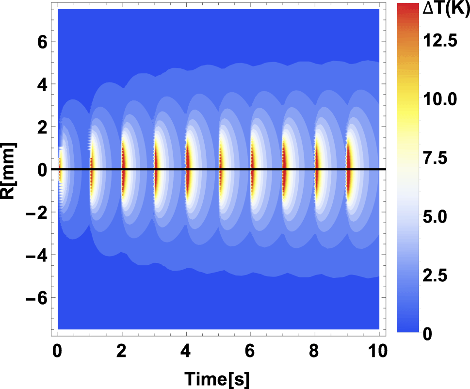
Figure 3.

Temporal evolution of the $z=0$ radial temperature distribution for a 1 Hz repetition rate pump. The time window ranges from 0 to 10 s, when the maximum temperature is reached. Color scale in kelvin. A maximum pump power was assumed (4 kW, 1 ms) delivered in a $w_{p}=1.35~\text{mm}$ waist radius, resulting in a temperature difference of 13.6 K between the edge and the center of the gain medium.

Figure 4.

Temporal evolution of the $z=0$ radial temperature distribution at 10 Hz, 1 ms pump pulse. Color scale in kelvin. (a) Time window corresponding to initial evolution (0–1 s), showing a net increase in the peak temperature. (b) Steady state at nearly constant temperature, with periodic fluctuations. Maximum temperature difference between the center and the coolant is 39.4 K.

The resulting periodic profile is given by the pump pulse arrivals and the evolution between them. On the other hand, at 10 Hz the time between two consecutive pulses is shorter than the thermal relaxation time, leading to a steady-state profile. This is achieved when an equilibrium is reached between the heat source term and the dissipation of the heat due to the built-up gradient. It was observed that the characteristic time of the steady-state formation is below 10 s, which was therefore taken as the upper limit for the simulations.

One should mention that while the influence of the heat removal was not addressed, previous works have shown a small influence on the temperature gradient, and thus, thermal lens power^{[Reference Chénais, Druon, Forget, Balembois and Georges14, Reference Loiko, Yumashev, Kuleshov and Pavlyuk24]}.

The time evolutions of the radial profiles for two regimes are presented in a contour plot form in Figure 3 (1 Hz pump rate, 10 s time window) and Figure 4, 10 Hz pump rate, for 1 s, at the beginning and the end of a 10 s interval, with the color scale being in kelvin. For an optical pump power of 4 kW, $w_{p}=1.35~\text{mm}$ and 1 ms pump pulse duration, the maximum temperature difference reached in the first case is $\unicode[STIX]{x0394}T=13.6~\text{K}$ (above the cooling temperature). By keeping the same optical pump profile and increasing the repetition rate to 10 Hz (in the second case) the steady state is attained at $\unicode[STIX]{x0394}T=39.4~\text{K}$.

2.2 Thermal lensing

The temperature profile discussed above can influence the laser gain medium and its performance within an amplifier in different ways, e.g., optical and mechanical deformations. In particular, those affecting the propagation of light through the introduction of wavefront distortions are (i) the direct change of the temperature-dependent refractive index and (ii) the deformation of the end-face curvature, effectively resulting in the formation of a transient lens caused by the relaxation of the thermally induced stress in the end regions.

In the case of a steady-state temperature, a constant thermal lens magnitude arises, and we are able to calculate its equivalent focal length. For this goal, we use a model presented in Ref. [Reference Baesso, Shen and Snook31], which, although being simple, has been shown to provide good estimates^{[Reference Lausten and Balling12, Reference Nadgaran and Sabaeian13, Reference Born and Wolf32]}. In this model, the space-resolved optical path difference (OPD) has a distribution between $z$ and $z+\text{d}z$ given by

(5)$$\begin{eqnarray}\displaystyle \unicode[STIX]{x0394}\text{OPD}(r) & = & \displaystyle \left[\frac{\text{d}n}{\text{d}T}+(n-1)(1+\unicode[STIX]{x1D708})\unicode[STIX]{x1D6FC}_{T}\right]\nonumber\\ \displaystyle & & \displaystyle \times \int _{0}^{l}[T_{\infty }(r=0,z)-T_{\infty }(r,z)]\,\text{d}z.\end{eqnarray}$$

The term $\text{d}n/\text{d}T$ is the refractive index thermal variation and is associated with thermal dispersion, and $\unicode[STIX]{x1D6FC}_{T}$ is the thermal expansion coefficient associated with the deformation of the rod surfaces, while $\unicode[STIX]{x1D708}$ is Poisson’s ratio.

Figure 5.

Optical path difference versus radial position inside gain medium for 1 Hz and 10 Hz. Quadratic behavior valid for the pumping region ($r<w_{p}=1.35~\text{mm}$). Significant differences shown for the outer region ($w_{p}<r<r_{0}=0.8~\text{cm}$).

The above integral was implemented numerically for the computational model. Figure 5 shows the corresponding results for different pumping conditions, valid for the pump waist region, alongside with a quadratic fit for a pump power of 4 kW and different repetition rates (1, 5 and 10 Hz). For a perfect lens of focal length $f$, the optical path difference is given by $\text{OPD}(r)=-r^{2}/2f$. The equivalent calculated focal lengths are $1.53\pm 0.03~\text{m}$ (10 Hz) and $5.04\pm 0.16~\text{m}$ (1 Hz). Outside the pumping region, the conduction process to the cooling system governs the temperature distribution, resulting in a smaller slope of the OPD. Therefore, higher order aberrations (i.e., deviation from the quadratic fit) will dominate^{[Reference Lausten and Balling12, Reference Loiko, Yumashev, Kuleshov and Pavlyuk24]}.

3 Experimental setup

In order to verify the validity of the previous numerical simulations, we assembled an experimental setup as shown in Figure 6, for characterizing the wavefront distortion introduced by an end-pumped crystal in a variety of conditions. An 8 mm long, 15 mm diameter Yb:YAG crystal is pumped by a maximum average power of 4 kW, 940 nm diode laser stack (Jenoptik). A set of cylindrical and spherical lenses is used to adjust the pump beam shape and size inside the crystal. The probe beam is sampled from a low-power laser oscillator operating at 1030 nm. The beam is frequency doubled in a BBO crystal, for improved wavefront resolution and to allow a better imaging contrast with respect to the pump beam. The probe beam is propagated through the crystal and directed by means of a reflective high-pass filter toward a high-resolution wavefront sensor based on quadrilateral wavefront shearing interferometry (Phasics model SID4). The incident beam propagates through the modified Hartmann mask, which results in its replication as four beamlets. The central plane of the crystal is imaged on the sensor, and a short-pass filter at its input prevents any pump radiation from leaking in. This system allows measurements with and without lasing conditions. The overall performance of the amplifier is shown in Figure 7. Maximum output powers of 100 mJ were achieved with lower than 4 kW input power.

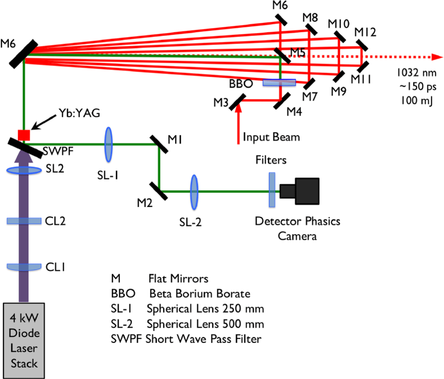
Figure 6.

Experimental setup for thermal lens measurement.

Figure 7.

Performance of the 8-pass amplifier. A maximum output energy of 100 mJ is achieved on a daily basis. The inset shows corresponding spectra for the main stages of the laser setup.

4 Results and analysis

Since the probe beam at the crystal plane exhibits a small (${\approx}0.35\unicode[STIX]{x1D706}$) wavefront curvature, this is taken as an input reference wavefront and subtracted via the sensor control software. It was verified that this consistently resulted in a nearly plane wave with negligible fluctuations (${<}0.02\unicode[STIX]{x1D706}$ peak to valley). Figure 8 shows the result of a typical acquisition, before (Figure 8(a)) and after (Figure 8(b)) removal of the reference wavefront, and after distortion introduced by the pump beam (${\approx}0.45\unicode[STIX]{x1D706}$) (Figure 8(c)). In the latter case, it is clear that the wavefront has become distorted in a lens-like form. The magnitude of this wavefront distortion is not negligible. In fact, it is comparable to the optical power of the original imaging system, which can lead to undesirable focusing in the beam path. The accuracy of the measurement system was tested using known focal length lens. Good correlations between measured and real values were obtained in a range from 30 cm to 5 m lenses.

Figure 8.

Wavefront measurements for the probe beam in units of $\unicode[STIX]{x1D706}$. (a) Input beam. (b) Residual wavefront after removal of the reference wavefront. (c) Example of a measured wavefront.

In order to retrieve the phase profile from the acquired image, the commercial sensor control software is used. It relies on the definition of a custom mask, after which the wavefront is projected onto a set of orthogonal wavefronts, the decomposition being unique. In the case of a circular pupil, as chosen, the Zernike polynomials act as the basic functions. In particular, the $Z_{3}$ polynomial, corresponding to defocus, can be related to the wavefront curvature induced by a perfect lens. By measuring the magnitude of this polynomial in the retrieved wavefront one can estimate the focal length of the induced thermal lens, by using the relation

(6)$$\begin{eqnarray}R=\frac{r_{p}^{2}}{4\unicode[STIX]{x1D706}Z_{3}},\end{eqnarray}$$

where $R$ is the calculated wavefront radius of curvature, $r_{p}$ is the pupil radius and $\unicode[STIX]{x1D706}$ is the probe beam wavelength. This radius of curvature can then be related to the focal length.

Figure 9.

Experimental thermal lens focal length versus pump power for 1 ms, 1 Hz (in red). Each data point represents the mean value of 10 consecutive measurements. The results of the numerical model are shown in black.

Taking this into account, we compared the experimental data obtained from the thermal lens measurements with the calculations described in the previous Section 2. As an example, Figure 9(a) shows a comparison of the results obtained with both approaches for a 1 ms, 1 Hz repetition rate pump. The measurements were taken under lasing and nonlasing conditions but no significant difference was observed, suggesting that the laser operation in these conditions is far from saturation and nonradiative effects are negligible.

The measurements are repeated for pump repetition rates of 2 Hz, 5 Hz and 10 Hz. The corresponding results are shown in Figures 9(b)–9(d). The theoretical model can estimate correctly the thermal lensing power for the range of parameters considered in this paper. The general evolutions of both curves match, with the absolute values differing by a factor of ${\approx}1.5$. We interpret these differences as a consequence of the establishment of a steady-state temperature profile in the first case, unlike in the second case. As previously discussed, the major contribution to the differences between the measured and numerically predicted values arises from the difference between the theoretical and experimental pumping profiles. The assumptions made should affect all the measurements in a similar way and future improvements on the model should include general pumping shapes. Additionally, at lower pump rates, due to shot-to-shot instabilities, oscillations in the wavefront lead to increased difficulties in measuring the wavefront curvature and associated errors. Another possible source of errors is the temporal triggering used for the experimental measurements. The retrieved values correspond to a time synchronization performed with the signal beam. It is a valid choice of triggering, due to the small time difference between pumping and signal (1 ms) compared with the thermal relaxation time (167 ms), but it can lead to small differences between the numerical and experimental data. It can be more significant in the case of a nonexistent thermal steady state, where the oscillations can be bigger. Nonetheless, given the assumptions that we have considered, the experimental and the calculated data agree remarkably well over a range of parameters. These results strongly highlight the importance of the thermal lensing effect, which can attain equivalent focal lengths of under one meter for high pump powers and repetition rates.