


Introduction
Increasing demands on the accuracy of solutions for glacier flow and improving computational possibilities are pushing the glaciological community to abandon the traditional shallow-ice approximation (SIA) (Reference HutterHutter, 1983) and include the computation of longitudinal stresses in numerical models. This is essential when the scaling assumptions of the SIA approach (Reference GreveGreve, 1997) are violated, such as for small alpine glaciers, ice streams, floating ice shelves, grounding-line dynamics and other, usually small-scale, examples of ice dynamics.
A number of theoretical and numerical approaches have been proposed and tested, including several higher-order approximations of the Stokes problem by ‘multilayer’ methods (Reference BlatterBlatter, 1995; Reference PattynPattyn, 2003; Reference Saito, Abe-Ouchi and BlatterSaito and others, 2003). For their classification and discussion see Reference HindmarshHindmarsh (2004). Also, a number of exact full-Stokes solvers have been developed, based on various numerical techniques such as finite-difference (e.g. Reference PattynPattyn, 2003), spectral (Reference HindmarshHindmarsh, 2004), finite-volume (Reference Price, Waddington and ConwayPrice and others, 2007) and finite-element methods (Reference Le Meur, Gagliardini, Zwinger and RuokolainenLe Meur and others, 2004; Reference Zwinger, Greve, Gagliardini, Shiraiwa and LylyZwinger, 2007; Reference Gagliardini and ZwingerGagliardini and Zwinger, 2008).
However, making the jump from the SIA approach to more advanced models substantially increases computational demands, which subsequently complicates the embedding of these techniques into large-scale models. In this paper, we present a computational algorithm that provides an approximate solution to the Stokes problem that is more accurate than the SIA solution, but still applies the traditional SIA scaling assumption on the aspect ratio of a glacier. The primary criterion for the construction of the new algorithm is computational efficiency.
The Stokes Problem for Flow
Our aim is to solve the boundary-value problem that allows us to model an incompressible Stokes flow with non-linear viscous rheology in a Cartesian geometry.
We are looking for the solution to the Stokes equation with the acceleration term neglected, that is, the linear momentum equation of the form

where ρ is the ice density,  is the gravity acceleration at Earth’s surface and the stress tensor,
τ
, is given by
is the gravity acceleration at Earth’s surface and the stress tensor,
τ
, is given by

where p and
σ
are the isotropic and deviatoric parts of
τ
, respectively, and I is the identity tensor. Since the ice flow is assumed to be incompressible and ice density homogeneous, the divergence-free constraint on the ice velocity,  , is to be satisfied:

A glacier is bounded by two continuously differentiable surfaces


where x 1, x 2, x 3 are the Cartesian coordinates. Considering the typical horizontal, [L], and vertical, [H], dimensions of a glacier, and typical horizontal, [V↔ ], and vertical, [V ↕], velocities of the glacier flow with the aspect ratio

the following scaling is introduced



where the scaling of the stress tensor is chosen as

Such a scaling only non-dimensionalizes the stresses, without requiring the scaled quantities to be of the order of unity, in which case a more appropriate scaling would be that suggested by Reference GreveGreve (1997).
The Stokes equation (1) for the scaled quantities reads as



where the symmetry of the deviatoric stresses, σ ij , was used and σ 33 was eliminated from the system of equations by making use of the trace-free constraint on the deviatoric stresses in such a way that only six independent stress unknowns are considered. The incompressibility condition (3) for scaled quantities then reads as

Boundary conditions
We assume stress-free conditions at the surface, i.e.

where  is the unit outer normal. In the scaled form, we have



at  .
.
At the glacier bed, we assume no-slip conditions, i.e.

or, in the scaled form,

Rheology
The connection between the deviatoric stress and the velocity is made by a rheological equation. Here we consider Glen’s flow law (e.g. Reference PatersonPaterson, 1981) (the Einstein’s summation convention is used if not otherwise stated):

where A is an ice flow parameter and  is given by
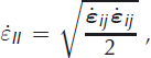
and
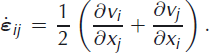
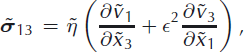
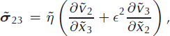
Applying the scaling, Equations (7–9), the rheology equation becomes
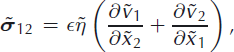
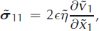
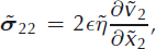
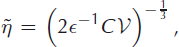

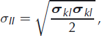
Inversely, the strain-rate tensor may be expressed in terms of the stress tensor as

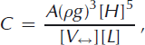
where
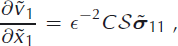
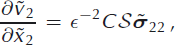
which, in the scaled quantities, reads as




The SIA-I Algorithm
In this section, we derive an iterative algorithm for updating velocity and stress fields based on the application of the Banach fixed-point theorem (e.g. Reference Granas and DugundjiGranas, 2003) for the ice-flow problem. The iterations start with the SIA-derived stress and velocity fields, which are then updated by solving an approximate problem that has more convenient numerical properties than the original setting. A crucial issue, convergence of the iterative algorithm, is ensured if the contractivity of the iterations holds. A detailed theoretical analysis of this question is not the subject of this paper, but the numerical examples presented in the following indicate that the algorithm converges for a wide range of ice-model parameters if the projection parameters controlling the iterations are chosen to be sufficiently small.
To derive the algorithm, let us consider the system of Equations (11–13) and assume there is an approximate solution in the kth iterative step, i.e. the field

The solution in the (k + 1)th iteration is constructed in a two-step procedure. In the first half-step, we find  as follows.
Denoting the exact solution of Equations (11–13) by  and defining the increment
  as
as

the system of Equations (11–13) for  may be rewritten as a system of equations for the increment
  , assuming that
  is known. We therefore obtain
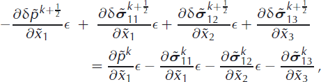
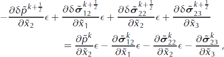
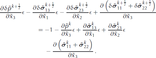
We now retain only the stresses  ,
,  and
and  in Equations (42) and (43) and the stress
  in Equation (44), and neglect all other terms on the lefthand sides of the equations. This approximation exactly corresponds to the traditional SIA approach, assuming that only the retaining stress components are dominant. Here, this approach is applied to the stress increments,
  , only, instead of the complete stress field as in the SIA (e.g. Reference GreveGreve, 1997). Hence, none of the stress components from the previous kth iterative step are omitted on the righthand sides of Equations (42–44). The SIA-like approximation results in the equations for the stress increments as follows
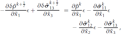
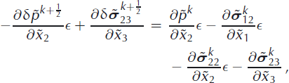
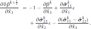
Equation (47) is now integrated along the vertical coordinate  , from the computation point
  to the boundary point
  which yields the pressure increment
  at the computation point
  . This result is then substituted into Equations (45) and (46) which, after integration along vertical coordinate,
  , gives the increments
  ,
,  at the computation point
  . The values of the integrands at
  are determined from the boundary conditions, Equations (16–18). To find them, the same procedure as before is applied. The exact solution is decomposed into the kth iterative-step solution,
  , and the increment
  , and only increments in
  ,
,  and
and  are retained to compensate for the discrepancy in adjusting the boundary conditions in the kth iterative step. After some algebraic manipulation, we obtain the boundary conditions for the increments in the form


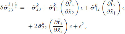
that are evaluated at  and we do not explicitly write the terms with ∊
2, because they will be excluded from the computations in the algorithm. Strictly speaking, this cannot be justified by the introduced scaling because we do not assume the scaled quantities and their spatial derivatives to be of order unity. What we present may hence be viewed as merely a formal procedure, which will be justified only by the final performance of the algorithm.
and we do not explicitly write the terms with ∊
2, because they will be excluded from the computations in the algorithm. Strictly speaking, this cannot be justified by the introduced scaling because we do not assume the scaled quantities and their spatial derivatives to be of order unity. What we present may hence be viewed as merely a formal procedure, which will be justified only by the final performance of the algorithm.
To sum up, the integration of Equation (47), followed by the integration of Equations (45) and (46), with the use of Equations (48–50), now results in the following formulae for the stress increments  ,
,  and
and  :
:
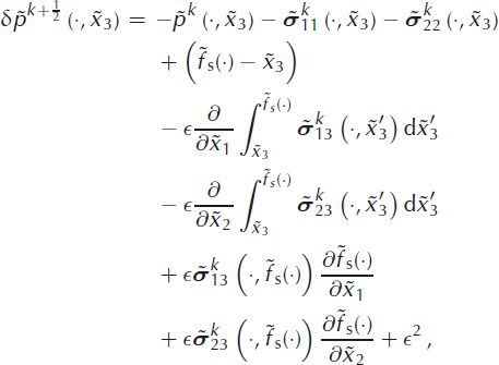
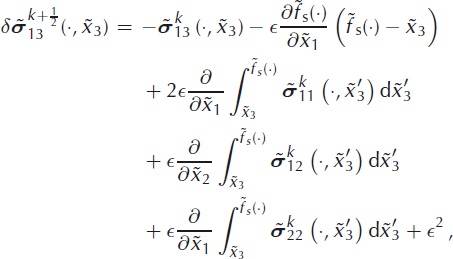
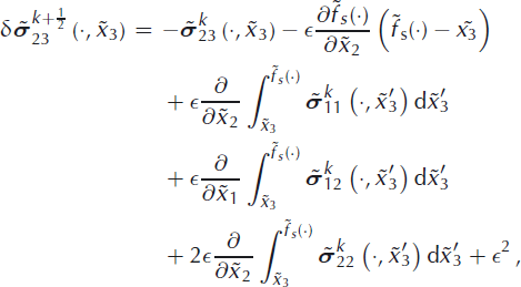
where the dot in (·) stands for the pair  for brevity and again terms with ∊
2 are not considered further and therefore not explicitly written.
for brevity and again terms with ∊
2 are not considered further and therefore not explicitly written.
We now define the updated solution in the  step as

where θ 1 ∊ (0, 1) is the first projection parameter of the iterative scheme. Note that, by the previous derivations, we consider

that is, only these three stress components are updated in the first half-step.
In the second half-step, the consistency of the stress field with the velocity field must be ensured, that is, the rheological equation must be adjusted.
First, the terms with ∊
2 on the lefthand sides of Equations (37) and (38) are neglected and the result is integrated along the vertical coordinate  from the glacier bed
  to the computation point
  . Making use of the no-slip boundary condition, Equation (20), and considering the updated stress field
  , we obtain


The velocity,  , is then obtained by integration of the incompressibility condition, Equation (14), from
  to
to  . Making use of the no-slip boundary condition, Equation (20), we obtain

This completes the determination of the velocity field  .
.
This field is now used to update the stress components from the rheological equation, that consequently reduces the inconsistency of the updated velocity field with stresses. The substitution of the velocity,  , into the rheological equations (24–31) yields the stress components that form a stress vector denoted by
  . The new
  is finally defined as a convex combination of the previous solution given by Equation (54) and the rheologically consistent solution
  , i.e. we define

where θ 2 ∊ (0, 1) is the second projection parameter of the iterative scheme.
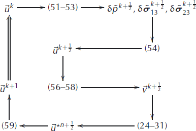
We call the presented approach that iteratively improves the SIA solution the SIA-I algorithm. Its computational steps may symbolically be depicted by the following scheme, starting from uk :
Numerical Simulation
In this section, we present numerical results obtained by the SIA-I approach for the ISMIP-HOM (Ice Sheet Model Intercomparison Project–Higher-Order ice-sheet Model) experiment (http://homepages.ulb.ac.be/∼fpattyn/ismip/).
Our approach has been incorporated into experiments A and B (model oso1) (see Reference PattynPattyn and others, 2008, for a discussion of results and model outputs). Here, we present the results for experiment A where the no-slip condition is considered at the glacier base. We also discuss the performance of the SIA-I algorithm for experiment C, where basal sliding with a prescribed sliding law is considered.
ISMIP-HOM experiment A
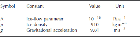
The problem is set up as follows. The experiment involves a Stokes flow problem, no slip at the bed, stress-free conditions at the surface and the ice is considered isothermal. The values of the physical parameters used are given in Table 1.
Values of physical parameters
The glacier has a square base of size [L] × [L]. The upper and lower surfaces are given (in meters) by


with

At the sides, the periodic boundary conditions are prescribed:


The plotted quantities are the velocities v 1, v 2, v 3 at the upper surface (in m a−1) and stress components σ 13, σ 23, Δp = p − Hρg at the bottom (in kPa), H = f s − f b. All quantities are mapped onto the scaled domain 〈0,1〉 × 〈0, 1〉. The numerical implementation includes the transformation of the problem into stretched coordinates, as usual in glaciology (e.g. Pattyn, Reference Pattyn2003). The glacier flow computed by the SIA-I approach is checked against a finite-difference full-Stokes solver (see Appendix). For a more detailed comparison with other solvers, see the results of the ISMIP-HOM experiment A (Reference PattynPattyn and others, 2008).
Results
Results for 

The SIA-I solution is computed with the projection parameters θ
1 = 0.2 and θ
2 = 0.05. The results are stored in a staggered grid of dimensions 41 × 41 × 41, where one type of node contains the velocity components  , while the other nodes contain the stress-tensor components
  and pressure
  . The SIA-I solution, obtained after 60 iterations, is shown in Figure 1 (full lines). The computation was performed on an Intel Pentium 4, 3.2 GHz computer and took ∼52 s. More details on the computational costs of the SIA-I are given below.
Comparison of the surface velocity fields (m a−1), and stress components,
σ
13,
σ
23, and the pressure difference, Δp = p − Hρg at the bottom (kPa), obtained by the SIA-I solver (full line labeled diagonally) and the full-Stokes solver (dotted line labeled horizontally), respectively, for the aspect ratio  .
.
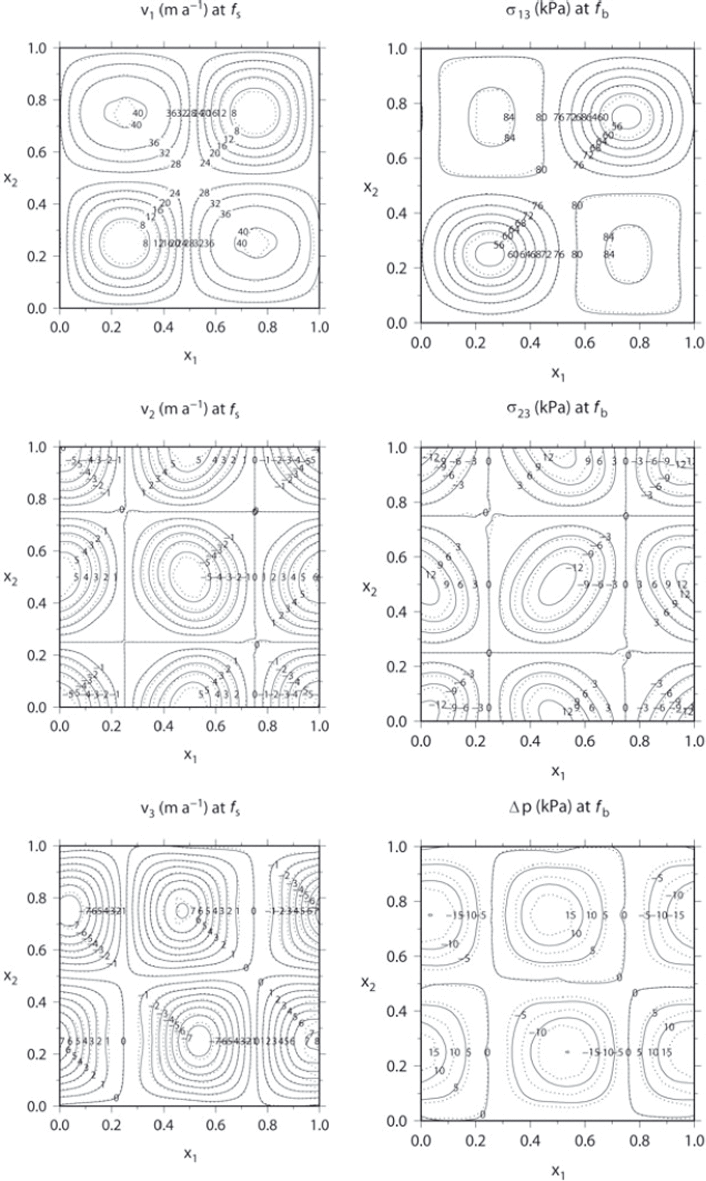
The full-Stokes solution (dotted lines in Fig. 1) was obtained by the standard finite-difference method (see Appendix). It was started from the SIA-I solution on a staggered 20 × 20 × 20 grid. The iterative updating of viscosity was stopped after 40 iterations, when the results were not changing within a specified tolerance. Figure 1 shows an almost perfect agreement between the SIA-I and finite-difference resulting surface velocities and a minor quantitative mismatch for the bottom stress components σ 13 and σ 23. The main difference appears, however, in the bottom-pressure difference, Δp.
Results for

The SIA-I solution is computed with the projection parameters θ 1 = 0.2 and θ 2 = 0.02. The resolution of the computational domain for both solutions was the same as in the previous case. The SIA-I solution, obtained now after 100 iterations to achieve the required tolerance (Fig. 2, full lines), is again compared with the full-Stokes solution (dotted lines) which was obtained by the finite-difference approach for 40 iterative updates of viscosity.
As for Figure 1 but for  .
.
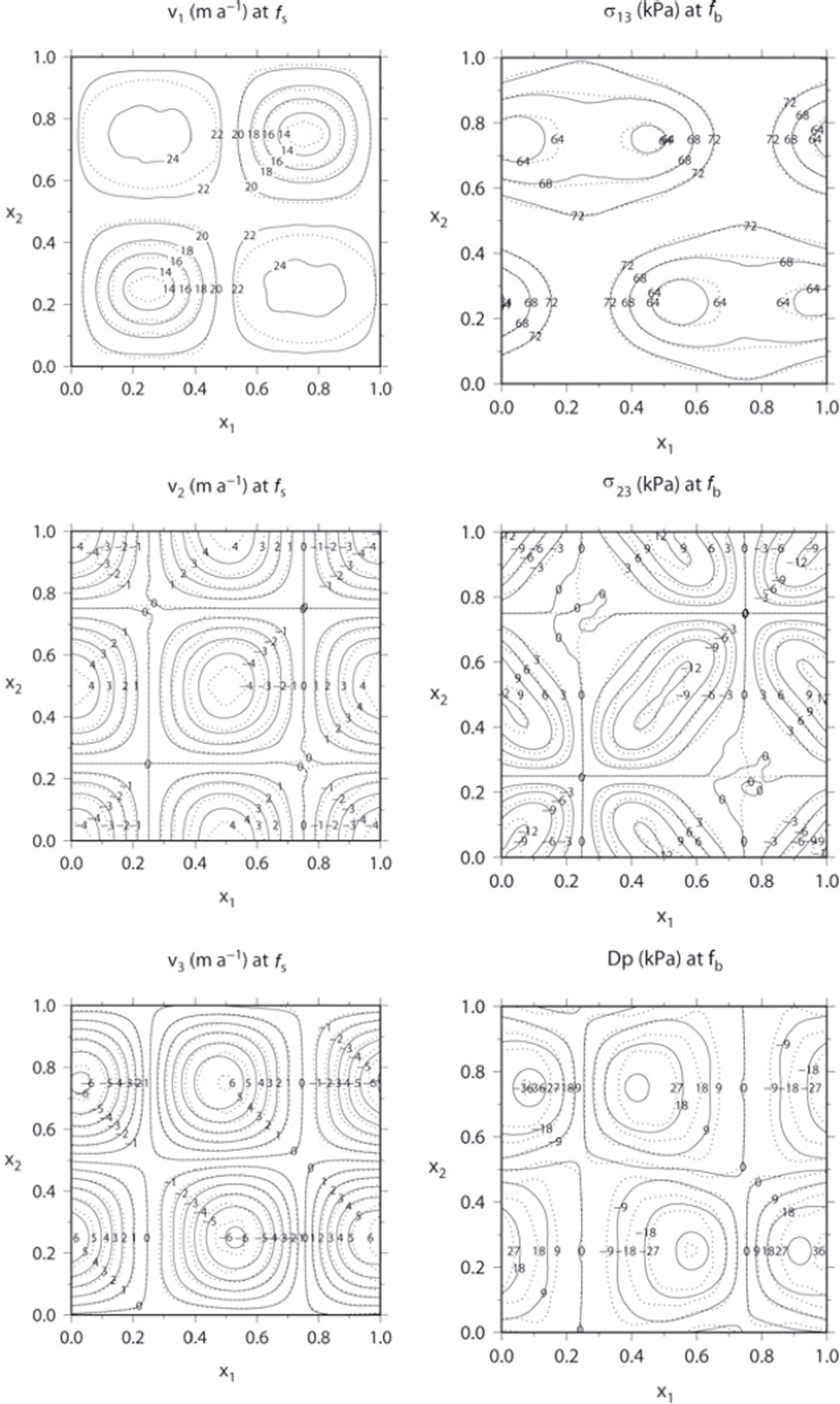
Inspecting Figure 2, we see rather good agreement between both the solutions, in particular for the velocities. Again, the largest difference appears in the pressure difference, Δp. It is noted that the SIA-I solution is smoother than the finite-difference solution, indicating possibly some numerical instabilities in the finite-difference solver.
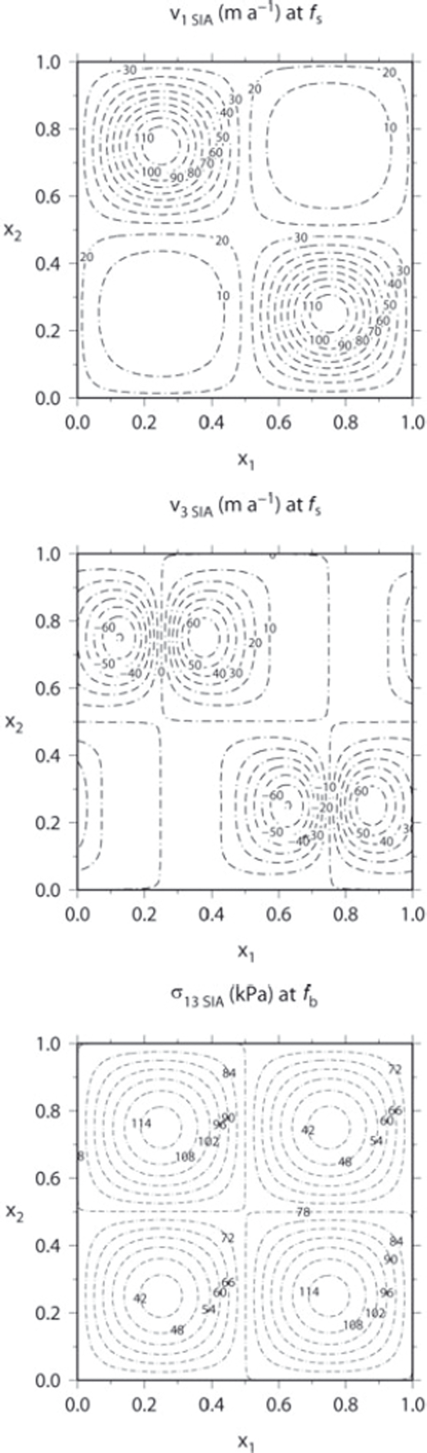
To estimate the order of improvement of the SIA-I solution compared to the SIA solution, Figure 3 plots the SIA solution for v1 and v3 at the surface (v2 is identically zero) and σ 13 at the bottom ( σ 23 and Δp are identically zero). Comparing Figure 2 with Figure 3, we see that the SIA-I solution differs significantly from the SIA solution, demonstrating that the SIA-I approach is capable of providing a more accurate solution of glacier flow.
The SIA solution for the aspect ratio  . Note that the field quantities not shown here (v
2 at f
s and Δp,
σ
23, at f
b) are identically equal to zero in this case.
. Note that the field quantities not shown here (v
2 at f
s and Δp,
σ
23, at f
b) are identically equal to zero in this case.
As demonstrated in the following section, the convergence of the SIA-I algorithm worsens with increasing aspect ratio, ∊. This can be overcome, to some extent, by choosing sufficiently small projection parameters θ
1, θ
2, but a threshold aspect-ratio value appears to exist for the practical usability of our method. For the current geometry setting from the ISMIP-HOM experiment A, this value is  .
.
Convergence of the SIA-I algorithm
In this section, we demonstrate how convergence is affected by varying the aspect ratio, ∊, and the magnitudes of the projection parameters, θ 1, θ 2. We perform all runs with the ISMIP-HOM experiment A set-up.
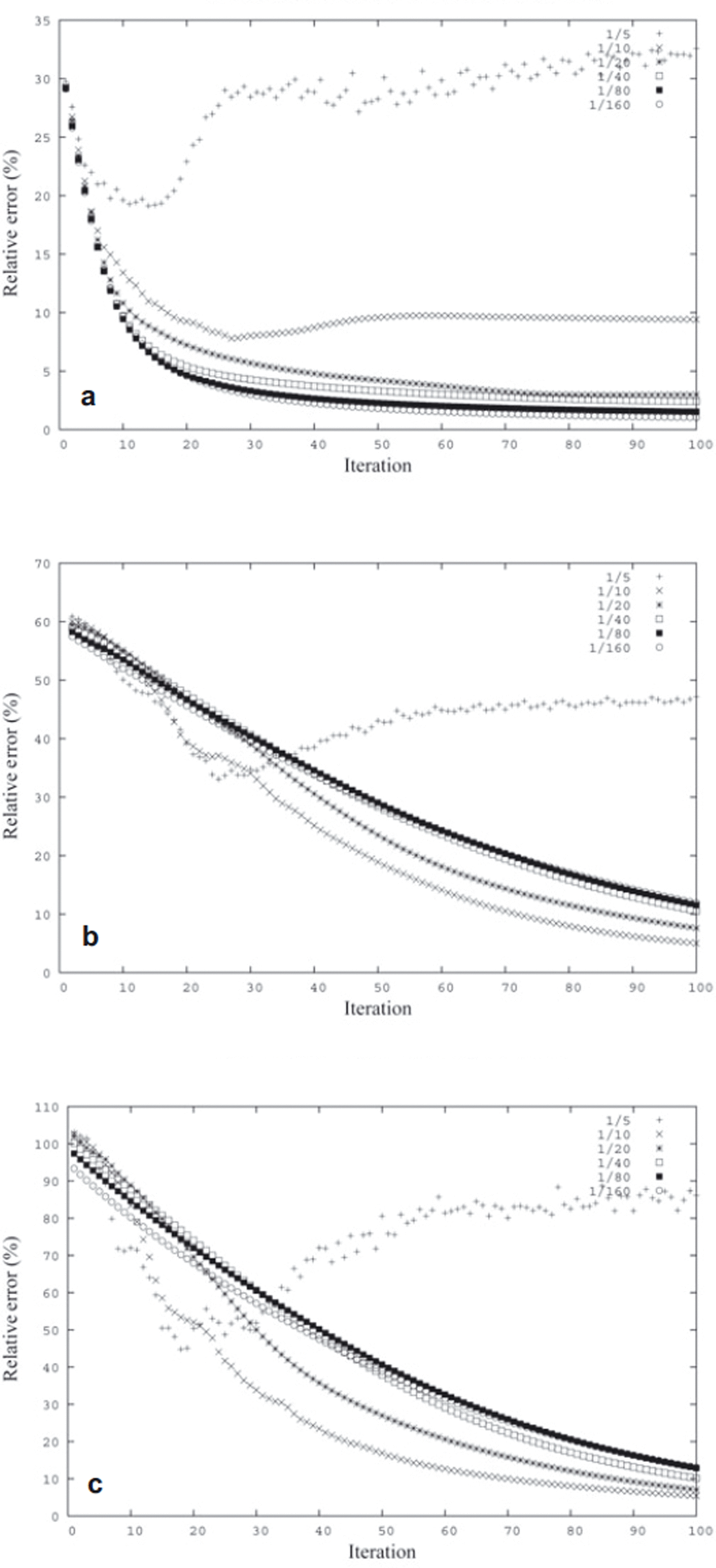
The convergence rate is inspected by checking the evolution of errors of linear momentum balances, rheology equations and equation of continuity, respectively. These errors are defined as follows. All the equations are evaluated at the nodes using the discretization of spatial derivatives by two-point symmetric finite differences. If we had an analytical solution, i.e. a solution satisfying the equations exactly in the limit of an infinitesimally small discretization, such a procedure would provide the so-called discretization error. In the case of the SIA-I solution, there is an additional approximation error, resulting from the fact that only an approximation to the full-Stokes problem is solved at each SIA-I iteration. We divide the error by the magnitude of the largest term in each particular equation and obtain the relative error at each node. For conciseness we first average these errors over the nodes and then compute one average value from the three linear momentum balance errors, one from the five rheology equations’ errors and finally one continuity equation error.
In Figure 4 we plot the total (discretization plus approximation) errors of the SIA-I solution for various combinations of the projection parameters θ
1 = 0.2, 0.5, 0.8, θ
2 = 0.2, 0.1, 0.05, a fixed aspect ratio,  , and spatial resolution 31 × 31 × 31. For all cases the overall error decreases and eventually reaches a limit (except for the uppermost curves in the middle and bottom panels, where more iterations would be needed to reach the limit). As documented for θ
1 = 0.8 and θ
2 = 0.2 (black triangles), when the projection parameters are chosen to be too large, the solution is scattered by a persistent high-frequency noise preventing the error from dropping below a certain value.
, and spatial resolution 31 × 31 × 31. For all cases the overall error decreases and eventually reaches a limit (except for the uppermost curves in the middle and bottom panels, where more iterations would be needed to reach the limit). As documented for θ
1 = 0.8 and θ
2 = 0.2 (black triangles), when the projection parameters are chosen to be too large, the solution is scattered by a persistent high-frequency noise preventing the error from dropping below a certain value.
The evolution of the averaged relative error of (a) linear momentum balances, (b) rheology equations and (c) equation of continuity, for various combinations of the projection parameters θ
1 and θ
2. The labels read as, for example, ‘0.2-0.05’: θ
1 = 0.2, θ
2 = 0.05. The results apply to the case of a spatial resolution 31 × 31 × 31 and aspect ratio  .
.
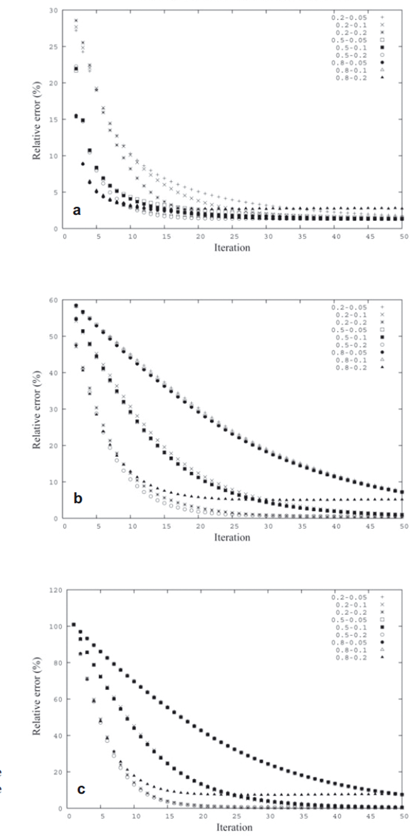
Observe that for, for example, θ 1 = 0.5 and θ 2 = 0.2, the error decreases relatively quickly and a sufficiently accurate solution is obtained after 20 iterations. We also see that below a certain critical value of the projection parameters, the convergence speeds up with their increase, while above the critical threshold the too-large projection parameters induce high-frequency scattering of the output. This may be connected to the spatial resolution since the sequence of successive iterative solutions may formally be viewed as a time-discretized evolution, and as the spatial dependency of field variables is also discretized by finite differences, one may expect a criterion, analogous to the Courant criterion (Reference Press, Teukolsky, Vetterling and FlanneryPress and others, 1992), to be fulfilled to ensure stability of the algorithm. For a given spatial resolution, this criterion would constrain the maximum values of the projection parameters, θ 1 and θ 2, that control the evolution in ‘time’.
Next, in Figure 5, we inspect the role of the aspect ratio, ∊. Since the derivation of the SIA-I approach requires ∊ be sufficiently small, there is a threshold value of ∊ above which the SIA-I algorithm will not converge. Figure 5 plots the errors for aspect ratios  and a fixed spatial resolution 31 × 31 × 31. The projection parameters are chosen as θ
1 = 0.2 and θ
2 = 0.02, for all computations. Figure 5 clearly demonstrates the key role of the aspect ratio, ∊, for convergence of the SIA-I algorithm. For the chosen projection parameters, θ
1, θ
2, the value
and a fixed spatial resolution 31 × 31 × 31. The projection parameters are chosen as θ
1 = 0.2 and θ
2 = 0.02, for all computations. Figure 5 clearly demonstrates the key role of the aspect ratio, ∊, for convergence of the SIA-I algorithm. For the chosen projection parameters, θ
1, θ
2, the value  is the threshold and for larger aspect ratios the algorithm fails to converge.
The evolution of averaged relative error of (a) linear momentum balances, (b) rheology equations and (c) equation of continuity, for various aspect ratios  and for a fixed spatial resolution 31 × 31 × 31. The results apply to θ
1 = 0.2 and θ
2 = 0.02.
and for a fixed spatial resolution 31 × 31 × 31. The results apply to θ
1 = 0.2 and θ
2 = 0.02.
In summary, whether the SIA-I algorithm converges and how fast it does so is a matter of several coupled factors. For a sufficiently small aspect ratio, ∊, (less than  for the ISMIP-HOM A experiment), the algorithm converges by choosing projection parameters, θ
1, θ
2, below certain threshold values, dependent on both the aspect ratio and the spatial resolution, and the convergence of the algorithm improves by approaching these critical values from below. Moreover, the critical values decrease with increasing aspect ratio, ∊; as a result, for
for the ISMIP-HOM A experiment), the algorithm converges by choosing projection parameters, θ
1, θ
2, below certain threshold values, dependent on both the aspect ratio and the spatial resolution, and the convergence of the algorithm improves by approaching these critical values from below. Moreover, the critical values decrease with increasing aspect ratio, ∊; as a result, for  it is impossible to reach convergence within the ISMIP-HOM A experimental set-up.
Performance of the SIA-I for other than the no-slip boundary condition, ISMIP-HOM experiment C
The SIA-I algorithm as described above may easily be modified to allow a Dirichlet boundary condition on the velocity at the glacier bed, that is the condition  . We merely modify Equations (56–58) as follows:



With this modification, the SIA-I algorithm was tested using real data from the Antarctic region, considering, in addition, temperature-dependent viscosity. Without presenting any results, we only state that, for a reasonably smooth Dirichlet condition on velocity at the glacier bed, the performance of the SIA-I approach is comparable to the no-slip case. We intend to publish details of this result in a future paper.
To involve the sliding at the glacier bed, it is, however, necessary to change the Dirichlet boundary condition to the Newton boundary condition. Although we have not participated in the ISMIP-HOM C experiment, we are still able to make a few remarks on the SIA-I performance for this case, when basal sliding is concerned.
The problem is set up similarly to experiment A, but the driving effect is, instead of bed-geometry undulations, spatial inhomogeneities in the basal-friction coefficient. The upper and lower surfaces are both inclined planes given (in meters) by

At the sides, periodic boundary conditions are again prescribed for the velocity field. At the glacier bed, the following sliding law is considered:

where  and
and  are the tangent and upward normal vectors to the glacier base, f
b, respectively. The sliding coefficient is given by
are the tangent and upward normal vectors to the glacier base, f
b, respectively. The sliding coefficient is given by

with

The Dirichlet condition on velocity, either in the form of no-slip or a prescribed velocity, is essential for the SIA-I algorithm since it allows a straightforward computation of the velocities by integration along the vertical coordinate. That is why the sliding law, Equation (67), has to be transformed to a Dirichlet-type condition for velocity. This can be done as follows. For β(·) ≠ 0, the stress field from the previous half-step can be used as
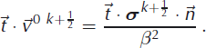
The sliding velocity,  , is then substituted in Equations (63–65) for
  . Evidently, this approach can only be applied to the region with β ≠ 0 while, in the region where β = 0, the algorithm fails. Such a situation occurs in the experiment C setting, where β = 0 at two points. To avoid the failure of the SIA-I approach, we add a small positive constant to β and successively decrease it during the iterations.
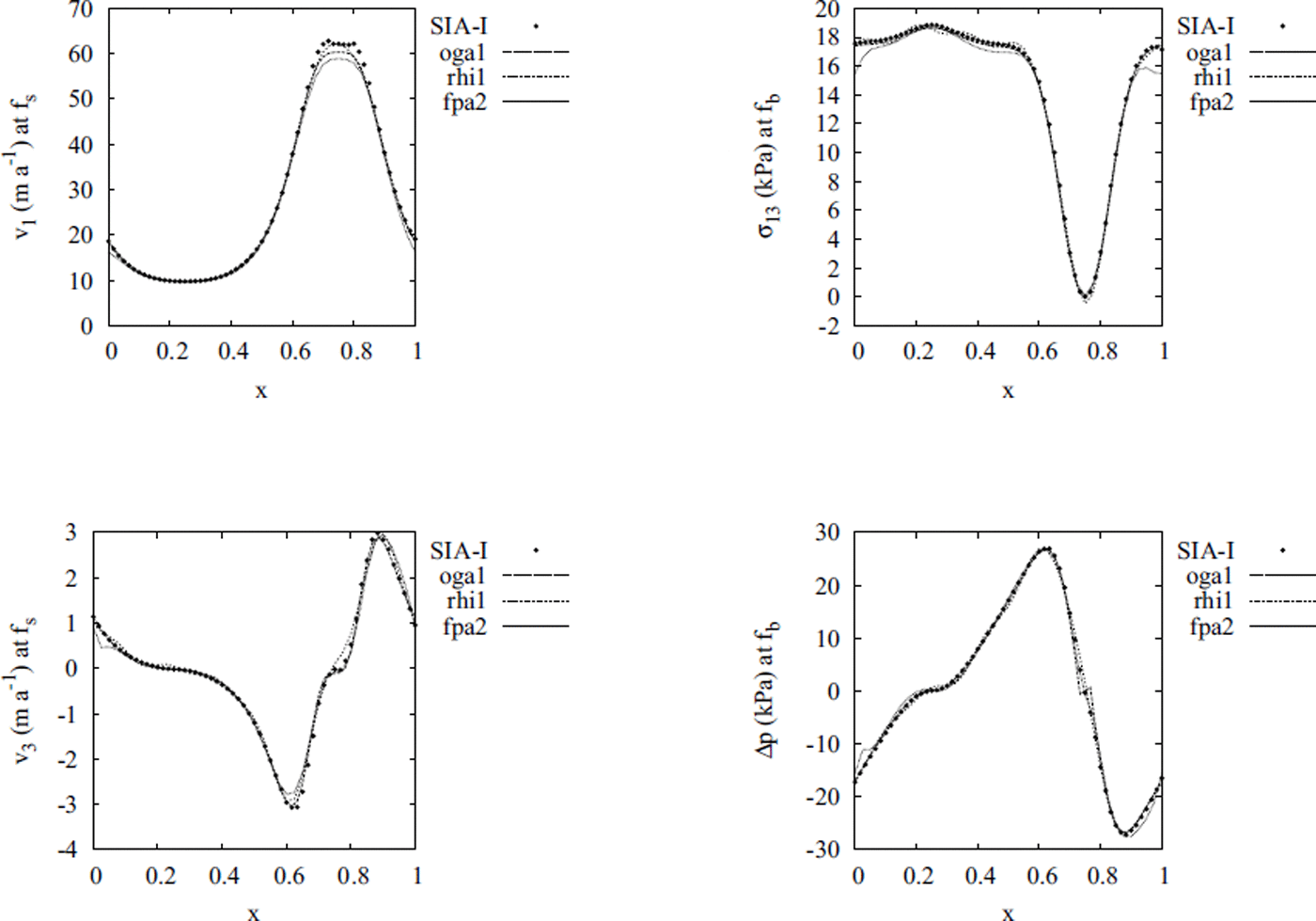
The results are shown in Figures 6 and 7. The plotted quantities are velocities v
1, v
3 at the upper surface (in m a−1) and the stress component,
σ
13, and pressure difference Δp = p − Hρg at the bottom (in kPa). As in the previous experiment, all these quantities are mapped onto the scaled domain 〈0,1〉 × 〈0,1〉 and the solutions are plotted at the cross-section with the plane y = 0.25. For the comparison, we plot three full-Stokes solutions from ISMIP-HOM experiment C, that is the models oga1, fpa2 and rhi1. We show the results for two aspect ratios,  in Figure 6, and
  in Figure 7. All solutions are computed with a resolution of 31 × 31 × 31, and are stopped after 200 iterations. The projection parameters are θ
1 = 0.2, θ
2 = 0.02 for aspect ratio
in Figure 7. All solutions are computed with a resolution of 31 × 31 × 31, and are stopped after 200 iterations. The projection parameters are θ
1 = 0.2, θ
2 = 0.02 for aspect ratio  and θ
1 = 0.1, θ
2 = 0.01 for aspect ratio
and θ
1 = 0.1, θ
2 = 0.01 for aspect ratio  . To compute each example takes 50 s of CPU time on an Intel Pentium 4 with 3.2 GHz.
Comparison of the surface velocity fields, v
1 and v
3 (m a−1), obtained by the SIA-I solver (black points) and the full-Stokes solvers oga1, rhi1 and fpa2 from the ISMIP-HOM C experiment, for the aspect ratio  . The displayed results are taken at an intersection of the scaled domain with the plane y = 0.25.
As for Figure 6, but for  .
.
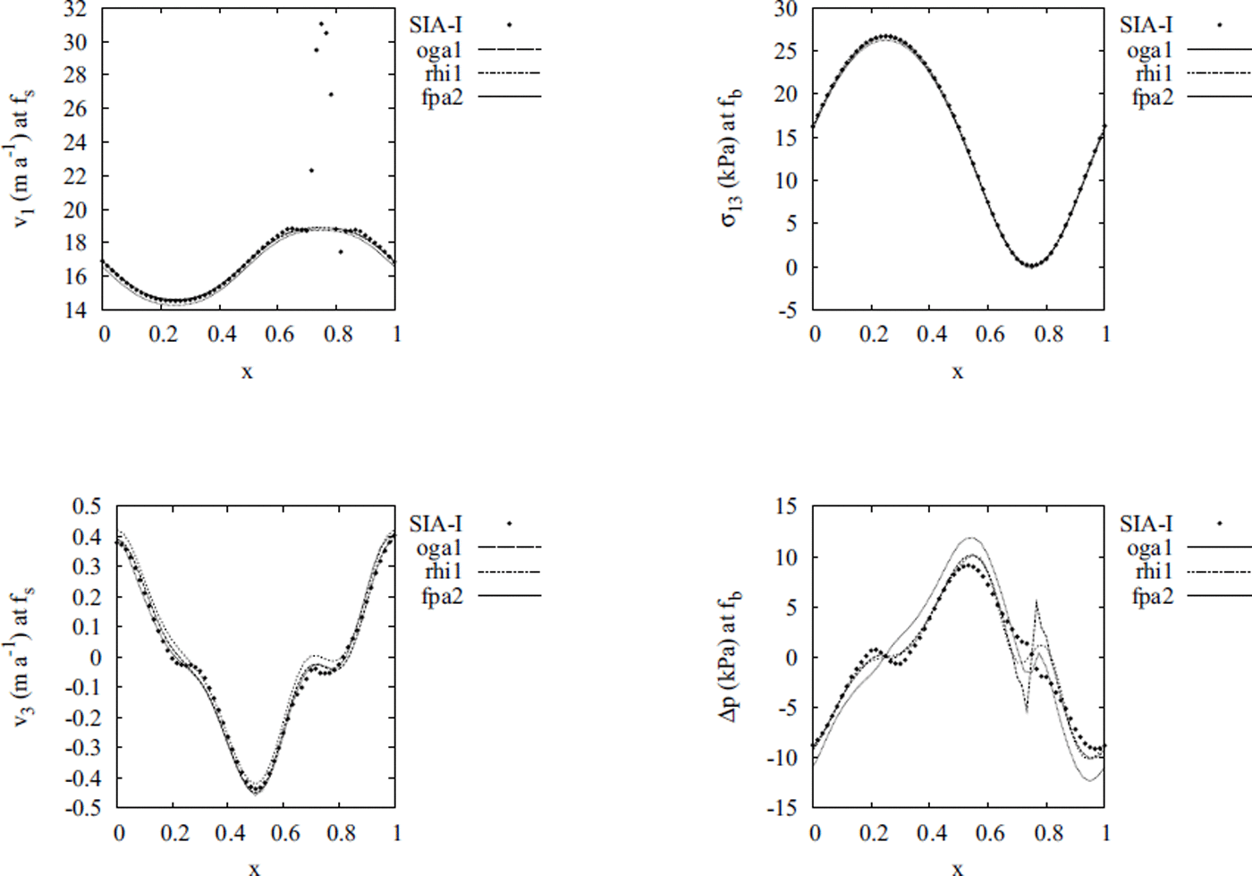
Figures 6 and 7 show that, in accordance with our assumption, the SIA-I algorithm fails to compute the horizontal velocities correctly in the neighborhood of the point where the sliding friction coefficient β = 0, that is at the point (0.75, 0.25) in our case. Moreover, the error increases with the increasing aspect ratio. However, the error is localized in a small region surrounding the point with β = 0, and the stresses are well computed everywhere, even for a relatively large aspect ratio  . In general, we may conclude that the Newton boundary condition at the glacier base, i.e. the sliding law of the form in Equation (67), represents a restriction for the applicability of the SIA-I only in the cases when the region of a very small basal friction coefficient, β, is present.
Numerical performance
The essential feature of the presented SIA-I approach is its computational effectiveness. The algorithm is designed such that the time cost spent at each iterative step is similar to that required for the SIA approach. Using an Intel Pentium 4, 3.2 GHz computer, we have performed 50 iterations for the ISMIP-HOM A setting with  , which is a sufficient number of iterations for the SIA-I solution to converge to the full-Stokes solution. In Figure 8 we plot the total CPU time for SIA-I as a function of degrees of freedom, that is the number of computed velocity and stress components on a staggered grid. We can see that computational time increases linearly with increasing number of degrees of freedom.
CPU-time demands of the SIA-I algorithm as a function of degrees of freedom for the ISMIP-HOM A setting with  and for 50 iterations, computed on Intel Pentium 4, 3.2 GHz.
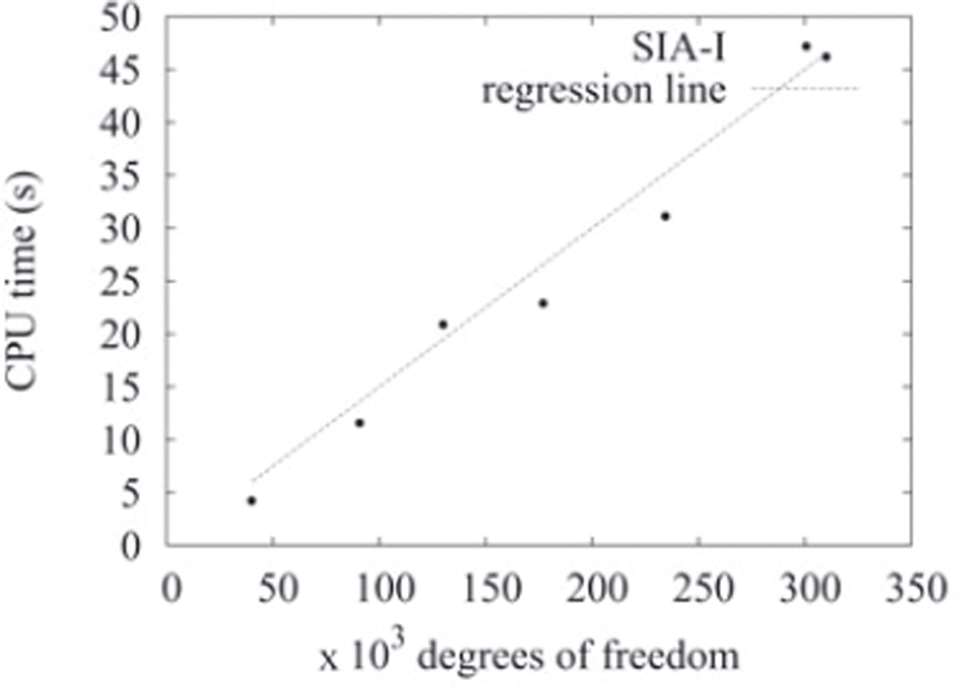
Since our full-Stokes solver is not optimized for numerical performance, we consider CPU-time demands for computational runs of the professionally optimized finite-element solver Elmer (Reference Gagliardini and ZwingerGagliardini and Zwinger, 2008). For the current ISMIP-HOM A setting, the authors provide an analytical formula for CPU-time costs in seconds as a function of the number of degrees of freedom: y = 0.013x 1.11. If we make a similar estimate for the SIA-I solver, we obtain y = 0.00015x (see Fig. 8).
Conclusions
The new iterative SIA-I algorithm presented in this paper is derived from the traditional SIA assumption of the smallness of the aspect ratio of the vertical/horizontal dimensions of a glacier. The algorithm represents an iterative extension of the SIA approach, and, in general, may provide a substantially improved solution of the Stokes flow problem. The key parameters controlling the performance of the SIA-I algorithm are the aspect ratio and projection parameters, θ
1, θ
2. For the model example taken from the ISMIP-HOM A experiment with  , the SIA-I algorithm converges if sufficiently small projection parameters are chosen. The case with
  is a threshold above which the SIA-I algorithm fails to converge, resulting in inaccurate and noisy results.
Besides its relative simplicity, the greatest advantage of the SIA-I algorithm is its fast computational speed, since it is designed such that the numerical computations consist of only numerical integration over the vertical coordinate and the differentiation of field quantities, similar to numerical operations performed within the SIA approach. Moreover, the computational demand grows only linearly with the number of degrees of freedom.
The performance of the SIA-I algorithm was also tested for the ISMIP-HOM experiment C where a Newton-type sliding law is applied at the glacier base. The SIA-I approach requires the reformulation of the sliding law as a Dirichlet boundary condition for velocity that results in wrongly computed velocities in the regions of small sliding friction coefficient, β. However, the errors in the velocities are localized in the vicinity of the region where β = 0. The erroneous behavior of the SIA-I algorithm disappears with decreasing aspect ratio. For instance, in the case where  , the SIA-I converges to the exact solution everywhere in the solution domain.
Acknowledgements
This work was supported by the Center for Earth Dynamic Research and also by the Grant Agency of Charles University in Prague through grant No. UK/252217. The second author acknowledges support from the Grant Agency of the Czech Republic through grant No. 205 /06/0580. Both authors thank F. Pattyn, R. Greve and an anonymous reviewer for constructive comments and K. Fleming for English corrections.
Appendix The Finite-Difference Full-Stokes Solver
To carry out the benchmarks against which the SIA-I solution could be checked, we developed a simple full-Stokes solver. The governing equations (11–13), (14) and (24–31) are rewritten in stretched coordinates (see, e.g., Reference PattynPattyn, 2003). The spatial derivatives are approximated by two-point symmetric differences and the resulting system of non-linear algebraic equations is solved on the staggered grid with two types of alternating nodes, first for the rheology equations and the equation of continuity, the others for the momentum balance equations. For a fixed viscosity, the linear system of equations is solved by a PARDISO (Parallel Sparse Direct Linear Solver) routine (http://www.intel.com), and the viscosity is iteratively updated by the convex combination of the previous and updated velocity fields. The convergence is checked by inspecting the evolution of the maximal difference between two successively computed velocity fields.



