1. Introduction

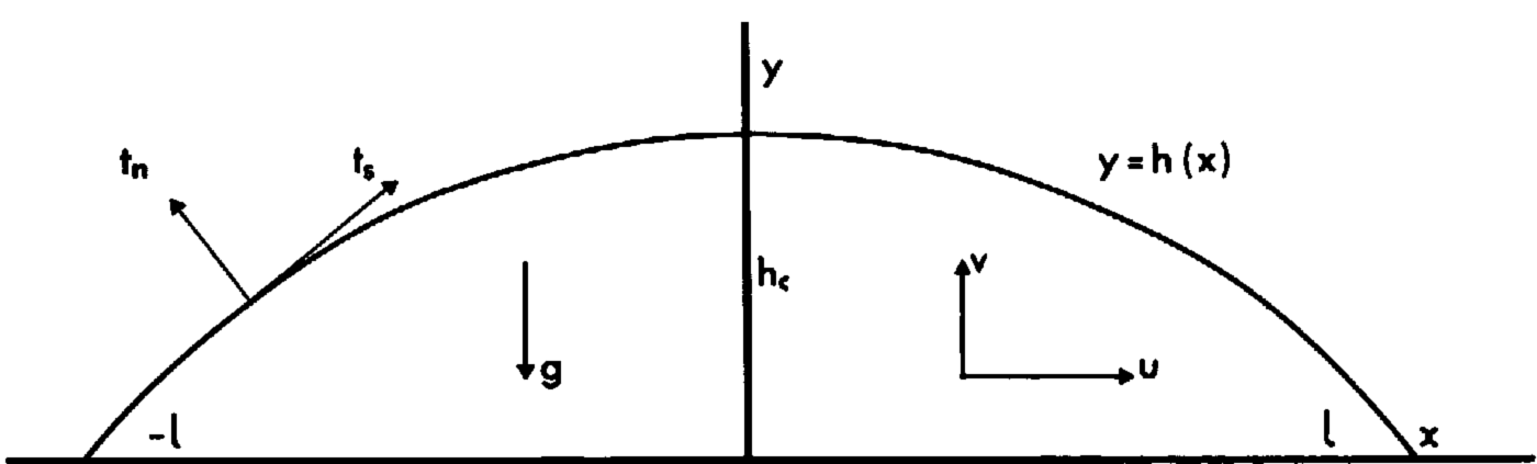
The first theoretical treatment of a bounded ice sheet with steady free surface, a property of the flow solution, was given by Reference NyeNye (1959). His basic problem was a two-dimensional symmetric ice sheet on a horizontal bed, in steady plane flow under gravity, with a steady profile maintained by surface accumulation and ablation. This is illustrated by the cross-section in Figure 1 with horizontal bed y = 0 and surface profile y = h(x) in rectangular Cartesian coordinates Oxyz, and all physical variables are independent of z. The velocity components are (u, v, o), g is the acceleration due to gravity acting in the negative y-direction, σ is the Cauchy stress tensor with σ _XZ = σ _yz = 0, and (t _s, t _n) denote tangential and normal tractions on the surface.

Fig. 1.

Ice-sheet cross-section.

Nye notes that in the ice sheets of Antarctica and Greenland the relative velocity between surface and bed is small compared with basal sliding, and, while the differential motion in glaciers is not negligible, it is largely concentrated in a thin basal shear layer. Using an estimated temperature profile with depth and a temperature-dependent flow law, Nye calculates the velocity and stress profiles under a point on the Greenland ice sheet, and concludes that any significant shear motion must be concentrated in the warmest layer at the bottom. He therefore proposes the approximation that the horizontal velocity is uniform with depth and is determined through a sliding law by the basal shear stress. In particular he makes the assumption

A and m are constants, which will depend on bed roughness, temperature, and basal ice structure; m = 2.5 is used for calculations. If a concentrated shear layer occurs near the bed, then (N1) applies at the base of the mean uniform velocity region. A rigorous derivation of a sliding law such as (N1) to describe mean flow conditions over a smoothed bed contour has yet to be found.

While Nye’s subsequent analysis is independent of the flow law and any temperature dependence, he has, nevertheless, deduced that observed temperature profiles give rise to an approximately uniform horizontal velocity profile above a thin bottom layer. In this paper we determine the horizontal velocity distribution by considering the full field equations, but on the assumption of uniform temperature so that Nye’s deduction can not be tested, nor can we predict the effect of temperature variation. However, our solutions demonstrate the errors produced by the same approximate procedure applied to the uniform temperature case, but more important is the presentation of a rational approximation scheme which appears to be appropriate to related free-surface problems involving other features, including temperature effects.

Nye next assumes that the surface slope is small, |h′(x)|⪡ 1, and approximates the basal shear stress by

where ρ is the uniform ice density. Equation (N2) is based on an equilibrium argument (Reference NyeNye, 1952), which supposes that the stress gradients parallel to the surface are negligible, and also implies σ _xx ≈ σ _yy Eliminating σ _xy between Equations (N1) and (N2), and expressing uh as the integrated surface accumulation by the assumption of incompressibility, gives a nonlinear first-order differential equation for h(x). For uniform accumulation q, Reference NyeNye (1959) obtains the solution

where

Thus, for given A, m, and q, the centre height h _c is related to the semi-length l, and either h _c, or l, or the aspect ratio h _c/l, must be specified to complete the solution. The assumption of constant q is inconsistent with zero net mass flux across the surface required for a steady profile, but Equation (N3) fails as |x| → l where the slope |h′| becomes infinite, and violates the basic assumption when |h′| is no longer small compared with unity, so there is an unspecified margin range with unknown profile where the necessary ablation takes place. Reference WeertmanWeertman (1961) also suggests that a requirement of slowly varying slope is implicit in Nye’s arguments, and is not satisfied by Equation (N3) in some central region. He further proposes that a non-zero effective longitudinal stress σ _xx —σ _yy can be accounted for by using a stress invariant in the boundary condition (N₁), by analogy with Glen’s three-dimensional constitutive law, but retains Equation (N2) and gives no further consideration to momentum or constitutive equations.

We have therefore re-examined the steady-motion-stcady-profile problem shown in Figure 1, treating the ice as a general non-linearly viscous fluid, prescribing the accumulation (ablation) as a function of the height of the free surface, prescribing basal drainage as a function of the overlying height of ice, and adopting a basal sliding law of the form of Equation (N1) but with a coefficient λ(h) depending on the overlying height of ice. Thus Equation (N1) is replaced by

Note that Equation (1) assumes that basal shear stress and velocity arc everywhere directed away from the centre. Basal drainage is described by

If q is the accumulation (volume flux per unit area) per unit horizontal cross-section, and q _n that per unit surface area, then

The normal form may be more appropriate on steep slopes, particularly for ablation zones q < o. Assuming that atmospheric pressure is uniform over the surface, and measuring stress relative to this isotropic pressure, the free-surface conditions are

The problem may be solved for x < 0 or for x > 0 by adjoining the symmetry conditions

Formulation of the full problem in dimensionless variables introduces a parameter ν, for which only a magnitude of h _c, not h _c itself, is prescribed in the definition. For a wide range of practical conditions ν ⪡ 1. The approximation ν = 0 gives a solution only for an unbounded sheet of uniform depth, not permitting a margin at finite distance l from the centre. This may be treated as an approximate solution valid in some central region—an “outer solution” in a matching procedure—but an intermediate scaling of the horizontal coordinate by a factor ε(ν) ⪡ 1 determines an approximate solution valid also in the central region. The parameter ε defines the small surface-slope magnitude, and is determined by the ice properties, accumulation magnitude, and magnitude of h _c. Further, this small-slope solution is valid up to the margin (h = o) provided that the sliding coefficient λ(h) ≃ λ _o h as h → 0. Here we present the leading-order small-slope solution under this validity condition. The central height h _c and semi-length l (and hence the aspect ratio, h _c/l) are determined by the solution, in contrast to Equations (N3) and (N4) where one parameter must be prescribed. From this leading-order solution Nye’s assumptions

and Equation (N2) are confirmed, but the profile, and consequently the shear stress and velocity distributions, are quite different from those of Reference NyeNye (1959) and Reference WeertmanWeertman (1961).

Illustrations are presented for Glen’s power law, the polynomial law of Colbeck and Evans, and a Newtonian fluid. The infinite viscosity at zero stress implied by the power law requires a more elaborate scaling procedure, but the analysis and solution are presented since the power law has become the conventional model. However, this model was introduced to describe overall response over a wide stress range, and not an accurate response near zero stress, and response functions which exhibit finite viscosity at zero stress arc probably a better physical description as well as leading to more straightforward analysis.

2. Balance laws and constitutive laws

Mass balance for an incompressible material implies

Inertia terms are negligible in this slow viscous flow so momentum balance requires

The ice is assumed to be an incompressible non-linearly viscous fluid with a temperature-dependent rate factor (Reference MorlandMorland, 1979). A convenient representation for use in Equation (9) is

where

and

T denotes temperature and a(T) is the rate factor, normalized by a(T ₀) = 1 for some temperature T ₀, with a′(T) ≥ 0. σ₀ and D ₀ denote a constant stress magnitude and a constant strain-rate magnitude respectively, so that

, the invariants Î ₂, Î ₃ and response functions Ø ₁, Ø ₂ are dimensionless. The alternative general representation for strain-rate in terms of deviatoric stress, given by Reference GlenGlen (1958), cannot be used to eliminate stress from Equations (9).

However, the laws commonly adopted for D give the simpler form

which implies

For example, with

Glen’s law deduced from uniaxial compression data is represented by

n depending on the stress range over which the response is approximated by this law. The singularity in ø ₁(Î ₂) as Î ₂ → o (J ₂ → o) implies an infinite viscosity at zero stress, and complicates the order of magnitude analysis of the problem described in Section 1. However, the analysis for such a singularity is presented since Glen’s law is the conventional model. More accurate data fitting over a low stress range suggests a finite viscosity at zero stress, and for 0 → 10⁵ N m⁻² Reference Colbeck and EvansColbeck and Evans (1973) propose a polynomial law represented by

ø(Î ₂) cannot be obtained by analytic inversion of Equations (14), but our leading-order solution can use Equations (16) or (17) directly.

From Equations (13) and (17) the viscosities at J ₂ = 0 and J ₂ = 1 (a deviatoric stress of 1 bar) are

and the mean viscosity commonly assumed for a Newtonian model near pressure melting is μ ≈ 3 × 10¹² N m⁻² s. As T decreases from T ₀, a(T) decreases from unity and the viscosity at each stress increases; at T = 250 K the viscosity is increased by a factor ten (Reference PatersonPaterson, 1969, p. 83), so a(250 K) ≈ 0.1. Increases are less pronounced for further decreases of temperature. In the subsequent analysis we assume a uniform temperature and take a = 0.1 for magnitude estimates. For a non-uniform temperature field the factor a[T(x)] introduces non-homogeneous response. In adopting the general law (10) we assume that the stress contribution from a non-zero ø ₂ term is not of greater magnitude than that of the ø ₁ term. Also it is assumed that ø ₂ is bounded, so |ø ₂| ≤ O(1), and ø ₁ can have a singularity only of the form given in Equations (16).

3. Dimensionless formulation and the small parameter

We introduce dimensionless variables by

where h ₀ is a magnitude of the maximum ice thickness (h _c = h ₀ H _c is determined by the solution, with H _c order unity), and q _m is a magnitude of maximum accumulation density, so P and Q are of order unity. We will suppose q _m = q(h ₀) on the assumption that ablation at lower heights does not significantly exceed this value; otherwise the ablation maximum should be used. We suppose that the drainage B is not greater in magnitude than Q. We can then define

Setting

in terms of a dimensionless stream function Ψ(X, Y), satisfies the mass balance Equation (8). The momentum Equations (9) become

Boundary conditions (1)—(6) become, for Y = 0:

for Y = H(X):

and for X = 0:

The tensors

have non-zero components

Taking a central accumulation q _m ≈ 3 × 10⁻⁹ m s⁻¹ (used by Reference NyeNye (1959) with h ₀ ≈ 3000 m), a rate factor a = 0.1, and the other variables taking the values given in Equations (15), gives

for a thick ice sheet and moderate glacier. In fact, with larger a and smaller q _m for a thin glacier, δ will be smaller than the larger value given in Equations (30), and the strong inequality δ ≤ 1 will apply in most, if not all, practical situations.

In Glen’s law (16), ø ₁ is unbounded as Î ₂ → 0 (n > 1), but ø ₁D → 0. For any singular ø ₁ of this form, we can write

where

and

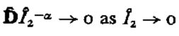
is bounded. For Glen’s law

and ø ₁ is constant, while the finite viscosity case is obtained by setting α = 0, with ø ₁ = O(1) by Equations (17). Hence Equations (31) and (32) cover both cases. From Equations (10) and (29),

where

For Glen’s law, Equations (33), with n = 1 corresponding to the finite viscosity case, and the parameter values given by Equations (15) and (30), the thick ice sheet and moderate glacier values of ν are shown in Table 1. Thus, recalling that a lower value of δ is expected for h ₀ = 100 m, and that n = 1 is the most realistic law, Table I implies

Table I.Magnitudes of ν and ε for a finite viscosity law (n = 1) and Glen’S law with exponent n

which is the condition we adopt. Note also that

is independent of h ₀, and decreases with decrease of q _m and increase of a. For practical conditions we can assume θ ≤ 0(1). Assuming that P, Ψ, and their gradients, are not greater than order unity, the leading order of a series solution in ν is given by setting ν = 0. In particular, from Equations (22) and (26),

which correspond to an unbounded sheet of uniform depth. That is, a margin at finite distance L cannot be obtained. Such a solution may represent an “outer” solution, valid in some central zone, to match with a solution which incorporates a surface slope, but as we now show that the indicated intermediate coordinate scaling leads to a solution uniformly valid to the centre, under a weak restriction on the sliding law, the ν expansion is not pursued.

4. Scaled variables and slope magnitude

For a non-zero surface slope, P, to leading order, must not be independent of X, so the horizontal momentum balance given by the first of Equations (22) must involve the shear-stress gradient in Y. This suggests a horizontal coordinate contraction

where ξ, γ = 0(1), and the slope Γ has magnitude ε. To retain the surface accumulation balance given by Equation (25), we need also a stream-function scaling

so Equation (25) becomes

Now, by Equations (29) and (34),

The terms of the first of Equations (22) now have orders of magnitude ε, νε ^{2α + 1}, νε ^{−1 δ 2α + 1}, νε ^{2α − 1}, νε ^{2α + 1} and a balance for the P-gradient with the shear-stress gradient requires

To satisfy the equality, take

Then the term in the inequality in (44) is ε^{θ(2α + 1) / (2 – 2α)} ≤ O(ε). Thus the ø ₂ term does not contribute to Σ _xx , Σ _yy to leading order with the assumption |ø ₂| ≤ O(1). Equations (45) show values of the ratio of the coordinate scale factor between n = 1 and n = 4, the extreme range, for a wide range of θ. Clearly the ratio is of order unity when θ is not too small or when n is close to unity. Table 1 shows the magnitudes of ε for the large and small h ₀ and various values of the exponent re. Again, n = 1 is the most realistic law, and smaller ν is expected for h ₀ = 100 m, so in most, if not all, practical situations,

From Equations (29), (42), and (45), we have the identity

5. Leading-order approximation

We now seek the leading-order approximation of a series expansions in ε. Let p = P ₀ + O (1), Ψ = Ψ₀ + 0(1) and

First derivatives of P ₀ and first to third derivatives of Ψ ₀ arise in the momentum balance, so these derivatives must be of order unity or less in a valid approximation. This is confirmed under weak restrictions on the sliding-law parameters. Denoting all leading-order quantities by a subscript or superscript o, we have

which confirm the magnitude relations (7). Recall that ø ₁, is evaluated at Î ₂ = θ ^1/(1-α)i₀, Î ₃ = 0.

The momentum balance Equations (22) become

On = 0, by Equations (23) and (24),

where

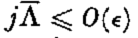
Λ is independent of n. This definition of Λ is normalized on the coordinate scale ε ₁ = ε(n = 1) to be independent of the exponent n used, and j is order unity except for n > 3 or θ < 10⁻²; j = 1 for n = 1. We suppose that the sliding law influences the leading-order solution, implicit in Reference NyeNye’s (1959) assumptions, so regard j Λ as order unity in the analysis. Perfect slip is given by Λ = 0, and non-slip by Λ = ∞. On ξ = 0, by Equation (28):

On Y = η(ξ), by Equations (26), (27), (49), and (41):

By the second of Equations (50) and the first of Equations (54),

Hence, by the first of Equations (50) and the second of Equations (54),

using Equations (32), (42), and (47). Thus the second of Equations (49) gives

which confirms Equation (N2). Now by Equations (49), Σ _xy ⁰ and δ²Ψ₀/δγ² have the same sign, and Equation (56) shows that this sign is unchanged at constant ξ, being the opposite sign to η′(ξ). In turn, Equations (51) shows that U ₀(ξ, o) has the opposite sign to η′/(ξ). Thus, for the sliding law given by Equation (1) with basal velocity directed away from the centre,

which imply monotonic profiles in ξ > 0 and ξ < 0 separately. Alternatively, monotonic profiles imply an unchanged sliding direction.

For laws of the form of Equations (13), using the relations (14),

which does not require explicit inversion of Equations (13). Given ø₁(Î₂, 0) in the general law given by Equation (10), Equation (56) must be solved for Î₂ to obtain the form of Equation (59). For Glen’s law (16), Equation (59) becomes

and for the polynomial law (17), for which α = 0,

A Newtonian fluid approximation with constant viscosity μ is given by Equation (60) or (61) with

For example, taking αμ = 3 × 10¹² N m⁻², based on Nye’s temperate viscosity, gives C ₀ = k = 0.33. In Equation (61), if θ ⪡ 1, the higher-power terms make little contribution, which implies that the deviatoric stress is much smaller than σ₀; that is |Σ _xy | |Σ _xx –Σ _yy | ⪡ s. By Equations (49) and (45), |Σ _xy |/s = 0(θ^{(1-2α)/(2-2α)}), so the shear stress only approaches 1 bar if θ ≈ 1; that is, q _m ∼ 3a × 10⁻⁷ m s⁻¹.

From Equation (59),

with g(t) given by Equation (60) for the power law and by Equation (61) for the polynomial law. Define

then integrating Equation (63):

Hence, by the second of Equations (51)

and by the first of Equations (51) and Equation (56)

Finally, the accumulation condition given by the third of Equations (54) on γ = η(ξ) gives

6. General properties and validity

We can rewrite Equation (68) as a first-order differential equation for η′(ξ) = γ ₀(η):

n = 1 is the finite viscosity case. This follows from the definitions (64) and Equations (60) and (61) for a power law and polynomial law respectively. Explicitly

Now

for zero mass flux, and the term in braces in Equation (69) is zero at γ₀ = 0 (ξ = 0), so must also vanish at η = 0 (ξ = ξ _m = εL) if Equation (69) holds over the entire range. This requires

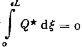
as η → 0.

As η → η _c = η(0), Λ(η) and Q*(η) are finite and γ ₀ → 0, so the essential behaviour of Equation (69) is

where l = min (m, n), ≥ 1. Hence

As η → 0 (0 ≤ γ ≤ η) or γ₀ → 0, the dominant terms of Ψ ₀, from Equation (65), are, in both limits,

Thus, as γ ₀ → 0, η →η _c,

Only derivatives ∂Ψ ₀/∂ξ and

(γ = 1, 2, 3) occur in the leading-order equations, but ∂ ²Ψ₀/∂ξ ², ∂ ²Ψ₀/δξ ∂Υ enter coefficients of higher-order terms in the stress expansions All are bounded as η → η _c for l ≥ 1. Anticipating, however, that ∂ ³ Ψ ₀/∂ξ ³ which arises in higher-order terms of the stress gradient must also be bounded, it is necessary that l ≤ 1, and hence |dγ ₀/dξ| ≤ O(1) which implies Reference WeertmanWeertman’s (1961) postulate of slowly varying slope. Direct differentiation of both terms of Equation (74) shows that bounded ∂ ³ Ψ ₀/∂ξ ³ requires (i) if l = n = 1 then, m = 1 or 2 or m ≥ 3; (ii) if l = m = 1 then n = 1 or 2 or n ≥ 3. It remains to determine the behaviour of γ ₀ as η → 0, and in particular to find any restrictions on m, n, β, and t to ensure that γ ₀ and appropriate Ψ ₀ derivatives are bounded.

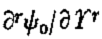
Let

which represents positive ablation plus drainage at the margin. If the first term within the braces in Equation (69) is dominant, then since 1 + m(1 + β — t) > 0 by Equation (71), the lowest power of η on the left-hand side of Equation (69) is β + m(1 + β − t), = 0 to balance the right-hand side; hence

The inequalities of (71) require

and t = 1 ⇔ β = 0. If the second term within the braces of Equation (69) is dominant, then β = − 1, which is not an acceptable solution. Now the first ξ derivative of the second term of Equation (74), applying Equation (77), ≃ η ⁻¹ if 0 < β < 1, and hence we require β = 0, t = 1, so that γ ₀ is analytic in η and third derivatives of both terms of Ψ ₀ are bounded with the previous restrictions on m, n. The power of η in the left-hand side of Equation (69) resulting from the second term is now (n+1)≥ 2, confirming that only the first term contributes to η ⁰ and η ¹. An explicit expansion shows that

Consider the solution of Equation (69) for −L/ε ≤ ξ ≤ 0 with Q*(η) such that the profile is monotonic: η′(ξ) ≥ 0, γ ₀(η) ≥ 0. The end condition given by the third of Equations (53) is

but η _c is a properly of the solution, being the height at which the net mass flux becomes zero:

Here we suppose Q* is negative near the margin, and increases monotonically with η into positive accumulation, and γ ₀ > 0 for 0 < η < η _c. However, Equation (81) is guaranteed for a valid solution under the restrictions (71), and Equation (79) prescribes the behaviour of γ ₀ at η = 0. Thus, we integrate Equation (69) from η = 0 and determine η _c explicitly as the height at which γ ₀ first becomes zero. The profile is determined by evaluating

bounded as η → η _c in view of Equation (73). In practice, the slope and profile are determined by numerical integration of the simultaneous differential equations

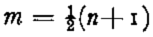
obtained from Equations (69) and (82) by using γ ₀ as independent variable. Starting at the margin we determine η = η _c and ξ = ξ _m = εL when γ ₀ = 0. Since β = 0, F(η, γ ₀) is defined explicitly at η = 0, γ ₀ = γ _m. Also λ = O(h) as h → 0 which is equivalent to λ being linear in the overburden pressure in view of Equation (55). The combination of linear dependence on height (pressure) and linear dependence on velocity (m = 1) was proposed by Reference BodvarssonBodvarsson (1955). So validity requires a “perfect slip” limit at the margin. Global perfect slip ³ ₀ ≡ 0 leads to γ ₀ ≡ 0 which is a uniform-depth solution with no margin. However, this may also be the leading-order solution for non-zero

which is valid in some central zone, and then the margin solution appears to have slope <O(ϵ) In practice a slope of order ε (or greater) at the margin is expected, so j Λ = O(1) is a reasonable assumption. In the non-slip limit Λ → ∞, Equation (69) gives β = −1, implying that a margin solution with slope greater than order ε (not necessarily unbounded) is needed. A new matched asymptotic expansion analysis is required to investigate this situation.

A Newtonian fluid solution is obtained by setting n = 1 in Equation (70) when Ω = ∓kηγ ₀. Then, with a linear sliding law (m = 1 ), (69) becomes (for ξ ≤ 0)

which has the explicit solution

since f(0) = 0, and Q* is negative at η = 0 and increases with η. Note that f(η) ≃ η as η → 0, since t = 1, so γ ₀ is finite. Thus γ ₀(η) and ξ(η) are determined by simple quadratures, and this evaluation was used to test the accuracy of the numerical integration of the differential Equations (83).

Reference NyeNye’s (1959) profile is deduced from constant accumulation q and constant λ. If we take q = q _m and λ = λ(n ₀), it is

independent of the ice law, and η _c unknown. Nye proposes

where n is the power in Glen’s law, then

By choosing η _c in Equation (87) as the central height determined by the preceeding solution for various cases, we can compare the profiles and ξ _m of Equation (87) with those of our leading-order solution. However, following Nye’s approximate procedure with general q(h), λ(h) leads to the differential Equation (69) with Ω ≡ 0; that is, the influence of the constitutive response is absent. It is clear from Equations (70) that when η and γ ₀ are not much smaller than unity, that is, away from the margin and centre, and j Λ(η) is not much smaller than unity, then the Ω term has the same magnitude as the sliding term, so omission of the Ω contribution is not justified.

7. Illustrations

For comparison between laws with different exponent n, we express all results in terms of the same dimensionless horizontal coordinate based on the scale factor ε₁ = ε(n = 1); that is, using Equations (45),

All calculations adopt the values (15) with a = 0.1, q _m = 3 ×10^-9 m s^−l, so that θ = 0.09 and the real slope magnitude ε for different n and h ₀ is shown in Table 1. In ξ < 0 the velocities are given by

where the subscripts b, s denote base and surface values, and

Both linear and exponential forms of the accumulation—drainage function Q*(η) and the sliding coefficient Λ(η) have been treated, namely

The exponential forms with large s and r imply small gradients Q*′ and Λ′ for η order unity, which correspond better with Nye’s constant Q*, Λ approximations than the linear functions. A case s = r = 5 is shown in Figure 2 together with an example using the linear forms, both with λ ₀ = Q ₀ = 1, comparing Nye’s profiles given by Equation (87) with the corresponding complete small-slope solution. As demonstrated earlier, the constitutive response term Q in Equation (69) cannot be neglected, but the examples in Figure 2 illustrate the entirely different profiles obtained with the further assumptions of constant Q* and Λ.

Fig. 2.

Comparison of small-slope profile for Glen’s law with Nye’s profile for λ ₀, = Q ₀ = 1.

(i)…… m = 1, n = 1, and exponential λ and Q*, s = r = 5.

(ii)____ m = 1, n = 1, and linear λ and Q*.

Next we indicate how the choice of constitutive law between the Colbeck and Evans polynomial law and Glen’s power law with n = 1 and n = 3 affects the solution. Table II shows values of the semi-length ξ _m* and height η _c for the linear forms of Equations (91) and (92) with m = 1, and λ ₀, Q ₀ between 1 and 10. The margin distance and centre height represent the maximum profile discrepancies. The greatest differences arise in ξ _m*, increasing with increasing λ ₀ for given law and given Q ₀. As Λ increases, the constitutive term has more influence, and the maximum differences in ξ _m* occur for λ ₀ = 10 with changes of 18 to 22% for the different Q ₀ between CE and n = 3. For moderate λ₀ the discrepancies are small, and the following illustrations are all based on the polynomial law, which eliminates the parameter n, and use the linear Q*(η) Λ(η).

Table II.Semi-length ξ_m*, height η_c , for linear accumulation Q*(η) and linear slidinc law (m = 1) with linear coefficient Λ(η). Solutions for Colbeck and Evans law (CE) and Glen’s law with n = 1, 3

Figure 3 shows profiles for four sets of (λ ₀, Q ₀, m). Increasing Q ₀ with λ₀ and m fixed decreases ξ _m* and increases η _c; that is, large ablation at the margin decreases the length as expected. Increasing λ₀ with Q ₀ and m fixed decreases ξ _m* significantly but makes little difference to η _c; that is, a larger “friction coefficient” decreases the horizontal spread. Similarly, increasing m with λ ₀ and Q ₀ fixed decreases ξ _m*. Figure 4 shows the basal velocity distributions for the same sets, all approximately linear on the normalized scale. The margin velocity is noticeably greater for the largest ablation, but the gradient along the base is not strongly influenced by change of λ ₀ or m.

Fig. 3.

Comparison of profile for Colbeck and Evans law with linear λ and Q*.

(i)_____ λ ₀ = 1, Q ₀ = 1, m = 1.

(ii)_____ λ ₀ = 1, Q ₀ = 5, m = 1.

(iii)…… λ ₀ = 5, Q ₀ = 1, m = 1.

(iv)_._._ λ ₀ = 1, Q ₀ = 1, m = 3.

Fig. 4.

Basal velocities |ε₁, U _b(ξ*)| corresponding to Figure 3 profiles.

Finally, Figure 5 shows both horizontal and vertical velocity distributions with height at various distances from the centre, for the case λ ₀ = 1, Q ₀ = 5, m = 1. ∂V/∂γ is nearly constant in both γ and ξ*, implying the same for ∂U/∂X by mass balance, and demonstrating that ∂V/∂γ and ∂U/∂X are both of order unity. While ε ₁, ∂U/∂γ small compared with unity except, perhaps, near the bed, it does not follow that ∂U/∂γ is small, and though the basal sliding velocity is much greater than the differential velocity between base and surface as noted by Reference NyeNye (1959), the contribution of ∂U/∂γ to the shear strain-rate, and hence the Ω term in Equation (69), is not negligible. Since ∂V/δξ* is order unity, the contribution δV/∂X is O(ε ₁), so ∂U/∂γ does indeed make a significant contribution. This highlights the need for a rational scaling of coordinates and physical variables to obtain the correct gradient balances in the field equation, and such scaling should be dictated by the boundary conditions or driving terms for the flow. Clearly our approach is appropriate to a variety of ice-sheet flow problems in which the driving mechanism suggests small-slope features.

Fig. 5.

Horizontal and vertical velocity distribution with height for linear λ and Q* with λ ₀, = 1, Q ₀ = 5, m = 1, at positions

(i) ξ* = −0.13 ______

(ii) ξ* = −0.63 _____

(iii) ξ* = −0.87 ……

(iv) ξ* = −1.04 _._._