2. The closure problem

Let us briefly review the mathematical model used in Souza et al.. The concentration field $\theta (\boldsymbol {x},t)$ of a passive scalar, advected by a random velocity field $\boldsymbol {u}(\boldsymbol {x},t)$, with constant scalar diffusivity $\kappa$ and a source $s(\boldsymbol {x})$, obeys the advection–diffusion equation

(2.1)\begin{equation} \partial_t \theta_{} + \boldsymbol{\nabla}\boldsymbol{\cdot}(\boldsymbol{u}_{}\,\theta_{} - \kappa\,\boldsymbol{\nabla}\theta_{}) = s(\boldsymbol{x}). \end{equation}

We can average this equation over realizations of the random field $\boldsymbol {u}$, and obtain an equation for the average $\langle \theta \rangle (\boldsymbol {x},t)$,

(2.2)\begin{equation} \partial_t \langle \theta\rangle + \boldsymbol{\nabla}\boldsymbol{\cdot}(\langle \boldsymbol{u}\theta\rangle - \kappa\,\boldsymbol{\nabla}\langle \theta\rangle) = s(\boldsymbol{x}). \end{equation}

The average here is an ensemble average over realizations of $\boldsymbol {u}$. The closure problem arises because in general we don't know how to deal with the term $\langle \boldsymbol {u}\theta \rangle$: (2.2) is not a closed equation for $\langle \theta \rangle$. The goal of a closure is to rewrite

(2.3)\begin{equation} \langle \boldsymbol{u}\theta\rangle = {O}[\langle \theta\rangle], \end{equation}

where ${O}$ is a linear operator, in general an integro-differential operator.

We isolate the issue by rewriting $\theta$ and $\boldsymbol {u}$ in terms of their ensemble mean and fluctuations:

(2.4a,b)\begin{equation} \theta_{} = \langle \theta\rangle + \theta_{}', \quad \boldsymbol{u}_{} = \langle \boldsymbol{u}\rangle + \boldsymbol{u}_{}'. \end{equation}

Then, subtracting (2.1) from (2.2), we find

(2.5)\begin{equation} \partial_t\theta' + \boldsymbol{\nabla}\boldsymbol{\cdot}( \boldsymbol{u}'\theta' - \langle \boldsymbol{u}'\theta'\rangle + \langle \boldsymbol{u}\rangle\,\theta' - \kappa\,\boldsymbol{\nabla}\theta' ) ={-}\boldsymbol{\nabla}\boldsymbol{\cdot}(\boldsymbol{u}'\langle \theta\rangle). \end{equation}

This last equation should be interpreted with care: on the left-hand side is a linear operator acting on $\theta '$, including the ensemble average $\langle \boldsymbol {u}'\theta '\rangle$, which can be expressed as

(2.6)\begin{equation} \langle \boldsymbol{u}'\theta'\rangle = \int \boldsymbol{u}_{\omega}'\theta_{\omega}'\,\mathrm{d}\mu_{\omega}, \end{equation}

where now we explicitly denote ensemble members by a subscript ${\omega }$, and the probability measure $\mu _{\omega }$ gives the relative weight of the ensemble member ${\omega }$. Equation (2.6) indicates that the left-hand side of (2.5) is an integro-differential operator involving the variables $({\omega },\boldsymbol {x},t)$, where ${\omega }$ itself could be countable to indicate an atlas of fixed velocity fields, or perhaps a continuous multidimensional variable that parametrizes the velocity field. Assuming that this operator is invertible (i.e. it admits a Green's function $\mathcal {G}_{{\omega }{\omega }_0}(\boldsymbol {x},t\,|\,\boldsymbol {x}_0,t_0)$), then the solution to (2.5) is

(2.7)\begin{equation} \theta_{\omega}'(\boldsymbol{x},t) ={-} \int \mathcal{G}_{{\omega}{\omega}_0}(\boldsymbol{x},t\,|\,\boldsymbol{x}_0,t_0)\, \boldsymbol{\nabla}_0\boldsymbol{\cdot}(\boldsymbol{u}'_0\langle \theta_0\rangle) \,\mathrm{d}\boldsymbol{x}_0\,\mathrm{d} t_0 \,\mathrm{d}\mu_{{\omega}_0}, \end{equation}

where a zero subscript denotes a function of $({\omega }_0,\boldsymbol {x}_0,t_0)$. Armed with (2.7), we can compute the flux $\langle \boldsymbol {u}'\theta '\rangle$. Souza et al. show that things simplify elegantly if we assume that the fluid is incompressible, $\boldsymbol {\nabla }\boldsymbol {\cdot }\boldsymbol {u}=0$ and that the statistics of $\boldsymbol {u}$ are stationary; in that case, let

(2.8)\begin{equation} \mathcal{K}(\boldsymbol{x}\,|\,\boldsymbol{x}_0) = \int \boldsymbol{u}'_{\omega} \otimes \boldsymbol{u}'_{{\omega}_0}\, \mathcal{G}_{{\omega}{\omega}_0}(\boldsymbol{x},t\,|\,\boldsymbol{x}_0,t_0) \,\mathrm{d} t_0 \,\mathrm{d}\mu_{\omega} \,\mathrm{d}\mu_{{\omega}_0}; \end{equation}

then

(2.9)\begin{equation} \langle \boldsymbol{u}\theta\rangle = \langle \boldsymbol{u}\rangle\langle \theta\rangle - \int \mathcal{K}(\boldsymbol{x}\,|\,\boldsymbol{x}_0)\boldsymbol{\cdot}\boldsymbol{\nabla}_0\langle \theta_0\rangle \,\mathrm{d}\boldsymbol{x}_0 =: {O}[\langle \theta\rangle]. \end{equation}

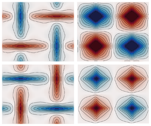
We have thus found the operator ${O}$ for the closure (2.3), with an ‘effective diffusivity operator’ given by $\int \mathcal {K}(\boldsymbol {x}\,|\,\boldsymbol {x}_0)\boldsymbol {\cdot }\bullet {\rm d}\boldsymbol {x}_0$. The case of an isotropic, purely local effective diffusivity is recovered when $\mathcal {K}(\boldsymbol {x}\,|\,\boldsymbol {x}_0) = \kappa _{{eff}}\,\delta (\boldsymbol {x} - \boldsymbol {x}_0)\,\mathbb {I}$, with $\mathbb {I}$ the identity tensor; clearly in general there is no reason to expect such a simple kernel. In fact the general kernel can even be non-symmetric, which indicates an induced drift, in addition to the mean drift $\langle \boldsymbol {u}\rangle$. Indeed, figure 1(a) depicts $\mathcal {K}(\boldsymbol {x}\,|\,\boldsymbol {x}_0)$ for a simple model system. If the effective diffusivity were purely local, the figure would show non-zero values only on the diagonal. We can see abundant coupling away from the diagonal, and the kernel is manifestly not symmetric.

Figure 1.

(a) A graphical representation of the kernel $\mathcal {K}(x,z\,|\,x_0,z_0)$ for a model flow, with $(x,z)$ unwrapped as a one-dimensional coordinate on each axis. (b) A comparison of the ensemble mean $\langle \theta \rangle$ computed using the exact equations, and with a local diffusivity approximation K, from (3.8). From Souza, Lutz & Flierl (Reference Souza, Lutz and Flierl2023).

As pointed out by Souza et al., a great benefit of (2.9) is that it is exact, given the model assumptions. For many applications, the form of (2.9) is probably too complicated to be of direct use. However, a proposed closure can now be couched as an approximation to $\mathcal {K}$, and having access to an exact expression should greatly help with validation. In an earlier recent paper, some of the same authors used this formalism to numerically compute the exact kernel $\mathcal {K}$ for a passive scalar in the ocean mixed layer (Bhamidipati, Souza & Flierl Reference Bhamidipati, Souza and Flierl2020).

3. A stochastic process and conditional means

In the present paper, Souza et al. probe the effective diffusivity kernel by computing it exactly for some model problems. Inspired by Hopf (Reference Hopf1952), their approach starts by specifying the ensemble ${\omega }$ as arising from a stochastic process ${\varOmega }(t)$, with a probability density $p_\alpha (t) = \mathbb {P}({\varOmega }(t) \in [\alpha,\alpha + {\rm d}\alpha ])$ that follows a master equation

(3.1)\begin{equation} \partial_tp_\alpha = \mathcal{L}_\alpha[p_\alpha] \end{equation}

for some generator $\mathcal {L}_\alpha$. Then they show that the weighted conditional mean

(3.2)\begin{equation} \varTheta_{\alpha}(\boldsymbol{x},t) = \langle \theta_{{\varOmega}(t)} \,|\, {\varOmega}(t) = \alpha\rangle\, p_\alpha(t) \end{equation}

obeys the equation

(3.3)\begin{equation} \partial_t\varTheta_\alpha + \boldsymbol{\nabla}\boldsymbol{\cdot}(\boldsymbol{u}_\alpha\varTheta_\alpha - \kappa\,\boldsymbol{\nabla}\varTheta_\alpha) = s(\boldsymbol{x})p_\alpha + \mathcal{L}_\alpha[\varTheta_\alpha]. \end{equation}

The mean is then recovered with $\langle \theta \rangle = \int \varTheta _\alpha \,\mathrm {d}\mu _\alpha$, as is the advective flux $\langle \boldsymbol {u}\,\theta \rangle$. Note that (3.3) itself is deterministic, even though there is an underlying random process, and is also autonomous – time does not appear explicitly and we are looking for a steady solution.

As a simple example, Souza et al. look at a stochastic Rossby wave system from Flierl & McGillicuddy (Reference Flierl and McGillicuddy2002), where the velocity $\boldsymbol {u}_\alpha$ is given by a stream function

(3.4)\begin{equation} \psi_\omega = \sin(x + \omega) \sin({\rm \pi} y),\quad (x,y) \in [0,1] \times [0,2{\rm \pi}], \end{equation}

where $\omega$ is a random phase angle, which obeys the stochastic process $\omega = \varOmega (t)$:

(3.5)\begin{equation} \,\mathrm{d}\varOmega = c\,\mathrm{d} t + \sqrt{2}\epsilon\,\mathrm{d} W. \end{equation}

Here $c$ is a constant angular velocity, and $W(t)$ is a standard Brownian motion. The master equation (3.1) is taken to be a Fokker–Planck equation

(3.6)\begin{equation} \partial_tp = \partial_\alpha({-}cp + \epsilon^2\,\partial_\alpha p). \end{equation}

The Fokker–Planck equation (3.6) together with (3.3), with source

(3.7)\begin{equation} s(x,y) = \sin (x)\sin({\rm \pi} y) + \cos(2x)\sin({\rm \pi} y), \end{equation}

can then be solved in various ways, for instance by discretization of the flow pattern into a finite set of states. Souza et al. extract an effective diffusivity operator, which can then be compared with the Taylor–Green–Kubo approximation for the local diffusivity (Taylor Reference Taylor1921),

(3.8)\begin{align} \boldsymbol{K} = \int_0^\infty \langle \boldsymbol{u}(\boldsymbol{x},t+\tau)\otimes\boldsymbol{u}(\boldsymbol{x},t)\rangle\,\mathrm{d}\tau = \tfrac{1}{4} \left[\begin{array}{@{}cc@{}} {\rm \pi}^2 \cos^2({\rm \pi} y) & - {\rm \pi}\cos({\rm \pi} y)\sin({\rm \pi} y) \\ {\rm \pi}\cos({\rm \pi} y)\sin({\rm \pi} y) & \sin^2({\rm \pi} y) \end{array}\right]. \end{align}

Figure 1 compares the ‘exact’ (numerically obtained) mean $\langle \theta \rangle$ with the mean obtained using the local diffusivity approximation (3.8). Indeed, there are visible deviations, indicating that the local approximation is flawed.

Of course, there remains an important problem: how to take a real time-dependent velocity field, either observed or numerically simulated, and model it as a series of random states. The authors discuss this by showing that what are essentially Koopman modes (Budišić, Mohr & Mezić Reference Budišić, Mohr and Mezić2012) can be used to break up a system into a discrete set of states. (Souza (Reference Souza2023) explores this idea further in a new preprint.) The strength of the current paper is that it builds a strong mathematical foundation for further study – after all, experience shows that ad hoc models are short lived and easily replaced, whereas models grounded in mathematics, even if imperfect, are revisited over and over again and eventually lead to significant breakthroughs. A precise definition of the effective diffusivity operator should help clarify the quality of a closure approximation, by testing in simple cases and then in more complex ones. Finally, a precise definition opens the way to more refined mathematical analysis, either by allowing a systematic use of asymptotics to derive closure models, or by providing an impetus for rigorous mathematical work.