





1. Introduction
Large pretrained language models (PLMs) have revolutionized the field of few-shot learning in natural language understanding (NLU). Few-shot NLU involves the challenge of learning a new task with only a limited number of labeled examples. This scenario is practical and relevant, as obtaining a small number of annotations is often feasible and training on such data is efficient. To harness the power of PLMs for downstream tasks (domain adaptation), prompt-based paradigms have emerged. These paradigms involve transforming the task into an LM-like objective using prompts. Prompts can be categorized into two types: discrete and continuous.
Discrete prompts, or hard prompts, pose a challenge due to the need for manual expertise in crafting effective templates, especially for specific tasks. ChatGPT, an advanced language model developed by OpenAI, has showcased remarkable proficiency across various natural language tasks reliant on hard prompt learning strategies (OpenAI 2023). To streamline this process, researchers have delved into devising automatic methods for prompt design (Lampinen et al. Reference Lampinen, Dasgupta, Chan, Mathewson, Tessler, Creswell, McClelland, Wang and Hill2022) and identifying the most informative few-shot examples (Wang, Yang, and Wei Reference Wang, Yang and Wei2024a) within hard prompt learning frameworks.
In the realm of pre-trained masked language models, strategies like language model-based fine-tuning (LMBFF) (Gao, Fisch, and Chen Reference Gao, Fisch and Chen2021a), PET (Schick and Schütze Reference Schick and Schütze2021b) and AutoPrompt (Shin et al. Reference Shin, Razeghi, Logan, Wallace and Singh2020) have been introduced to unearth effective prompts. However, while these automated techniques offer promising avenues, they might not consistently pinpoint the optimal prompts and often necessitate a substantial amount of validation data to validate their efficacy.
Soft prompts, also referred to as continuous prompts (Liu et al. Reference Liu, Zheng, Du, Ding, Qian, Yang and Tang2024), provide a means to simplify the search for effective prompts in downstream tasks. These prompts are learnable parameters that can be inserted into the input and optimized based on the task objectives and few-shot examples. Soft prompts do not require manual design or fixed input formats while they usually treat the underlying PLM as a black box. Using soft prompts gives us the extra advantage of avoiding the human bias injection that can be caused by manually designed prompts (Tian et al. Reference Tian, Emerson, Miyandoab, Pandya, Seyyed-Kalantari and Khattak2023). Notably, two methods that leverage soft prompts that see PLM as a black box and achieve remarkable few-shot performance are differentiAble pRompT (DART) (Zhang et al. Reference Zhang, Li, Chen, Deng, Bi, Tan, Huang and Chen2022) and PTuning (Liu et al. Reference Liu, Ji, Fu, Tam, Du, Yang and Tang2022). DART combines a DART mechanism with a fluency constraint objective, ensuring that the prompt tokens are compatible with the PLM’s prior knowledge and preserve the LM information during task learning. We evaluate our contributions on DART and PTuning as our base models in this work because (i) their implementation is publicly available and (ii) their additional objectives are applied to the output representations and the inner layers of PLMs are not needed.
Contrastive learning is a technique that enhances the robustness of various models against biases and distribution shifts by creating robust representations (Chen et al. Reference Chen, Xie, Bi, Ye, Deng, Zhang and Chen2021; Choi et al. Reference Choi, Jeong, Han and Hwang2022; Pan et al. Reference Pan, Hang, Sil and Potdar2022; Sahoo et al. Reference Sahoo, Panda, Senapati, Das, Kim and Feris2023; Du et al. Reference Du, He, Zou, Tao and Hu2024). Lately, supervised contrastive learning (SCL) (Gunel et al. Reference Gunel, Du, Conneau and Stoyanov2020) has demonstrated improvements in supervised learning, especially in few-shot setups (Gunel et al. Reference Gunel, Du, Conneau and Stoyanov2020; Jian, Gao, and Vosoughi Reference Jian, Gao and Vosoughi2022; Abaskohi, Rothe, and Yaghoobzadeh Reference Abaskohi, Rothe and Yaghoobzadeh2023). However, it has not yet been applied to soft prompt learning methods.
In this paper, we study the effects of incorporating SCL into our two soft prompt learning models, DART and PTuning. Our implementation of SCL does not require data augmentation but instead leverages the existing examples within a batch, following similar approaches to Gunel et al. (Reference Gunel, Du, Conneau and Stoyanov2020) and Zhang et al. (Reference Zhang, Ji, Ji and Wang2022). Additionally, we propose a novel approach called balanced batch in SCL (BBSCL), which employs batch-balancing techniques to further enhance the robustness of SCL, particularly in label-imbalanced settings.
LLMs offer a valuable resource for data generation, particularly in tasks where human performance is outstanding and the models have been proficiently trained. However, they may struggle with generating suitable outputs for novel tasks (Møller et al. Reference Møller, Dalsgaard, Pera and Aiello2023). Data augmentation, while commonly used, can distort the original distribution of real data, potentially compromising the quality of model training (Suhaeni and Yong Reference Suhaeni and Yong2024). Considering the costs associated with LLM usage, including GPU and API expenses, as well as the limitations posed by models like ChatGPT, it becomes imperative to enhance model performance under imbalanced few-shot learning scenarios without resorting to data augmentation. This aspect underscores the significance of our work, as we seek to improve model robustness without resorting to conventional data augmentation techniques.
We conduct experiments on thirteen NLU tasks, namely SST-2, MR, CR, Subj, TREC, MNLI, SNLI, QNLI, MRPC, QQP, Overruling, TC, and ADE. Our experimental results consistently demonstrate that including SCL in soft prompt models leads to improved performance compared to our base models. To further evaluate the effectiveness of our contributions, we specifically assess the impact of adding SCL and the BBSCL extension on three few-shot label-imbalanced settings. Our findings indicate that SCL is effective in these scenarios as well, and the introduction of the BBSCL extension further enhances the robustness of the models. Moreover, we delve into the analysis of SCL’s impact by examining the relationship between label complexity and its performance contribution. Notably, we observe that SCL tends to yield higher performance gains in cases where the label space is more complex and characterized by less separable classes. Our work makes the following key contributions:
-
• Integrating SCL into soft prompt tuning frameworks (DART and PTuning) for few-shot NLU tasks.
-
• Proposing BBSCL, a novel method to stabilize SCL in label-imbalanced settings through balanced mini-batches.
-
• Comprehensive empirical validation across 13 tasks, including real-world datasets, showing average gains of $2.1\%$
over base models.
$2.1\%$
over base models. -
• Demonstrating that SCL’s benefits are pronounced in complex label spaces and that small PLMs with our methods outperform large LLMs like GPT-3.5 in imbalanced scenarios.

2. Related work
2.1 Soft prompt learning
Soft prompt learning and its variations, such as prompt-tuning and residual prompt tuning, are emerging techniques aimed at enhancing the performance of PLMs with minimal parameter updates. These methods are designed to be both efficient and effective, leveraging the existing knowledge within large models to adapt to specific tasks.
Works like PTuningV2 (Liu et al. Reference Liu, Ji, Fu, Tam, Du, Yang and Tang2022), prefix-tuning (Li and Liang Reference Li and Liang2021), CodePrompt (Choi and Lee Reference Choi and Lee2023), and SwitchPrompt (Goswami et al. Reference Goswami, Lange, Araki and Adel2023) use soft prompt learning, but they do not see PLMs as a black box. they add parameters in PLM layers for tuning.
Residual prompt tuning significantly enhances standard prompt tuning by incorporating a shallow network with a residual connection, improving performance and stability across various tasks, including the SuperGLUE benchmark. Additionally, it demonstrates reduced sensitivity to hyperparameters such as learning rate and prompt initialization (Razdaibiedina et al. Reference Razdaibiedina, Mao, Khabsa, Lewis, Hou, Ba and Almahairi2023). However, this model does not assess robustness in imbalanced scenarios and is developed based on label text generation, differing from encoder PLMs. Therefore, our SCL extensions, which focus on input representation, are not accommodated by this model. Decomposed prompt tuning (DePT) (Shi and Lipani Reference Shi and Lipani2024) improves performance and reduces memory and time costs by over $20\%$
compared to standard prompt tuning, while maintaining competitive performance with fewer trainable parameters. XPrompt (Ma et al. Reference Ma, Zhang, Ren, Wang, Wang, Wu, Quan and Song2022), a novel prompt tuning model, bridges the performance gap between prompt tuning and fine-tuning at smaller model scales by eliminating negative prompt tokens through hierarchically structured pruning. Like residual prompt tuning, DePT and XPrompt do not evaluate model robustness in imbalanced scenarios and are also based on label text generation, which is distinct from encoder PLMs. Thus, it does not meet the requirements of our SCL extensions.
$20\%$
compared to standard prompt tuning, while maintaining competitive performance with fewer trainable parameters. XPrompt (Ma et al. Reference Ma, Zhang, Ren, Wang, Wang, Wu, Quan and Song2022), a novel prompt tuning model, bridges the performance gap between prompt tuning and fine-tuning at smaller model scales by eliminating negative prompt tokens through hierarchically structured pruning. Like residual prompt tuning, DePT and XPrompt do not evaluate model robustness in imbalanced scenarios and are also based on label text generation, which is distinct from encoder PLMs. Thus, it does not meet the requirements of our SCL extensions.
The transferability of trained soft prompts to similar tasks can accelerate training and improve performance, with cross-task transferability generally being more effective than cross-model transferability (Su et al. Reference Su, Wang, Qin, Chan, Lin, Wang, Wen, Liu, Li, Li, Hou, Sun and Zhou2022). The performance of prompt tuning can be highly sensitive to the initialization of prompts, and traditional methods may not encode sufficient task-relevant information (Wu et al. Reference Wu, Yu, Wang, Song, Zhang, Zhao, Lu, Li and Henao2023).
The meta soft prompt approach effectively generalizes PLMs across multiple domains, facilitating rapid adaptation to new domains through few-shot unsupervised domain adaptation (Chien, Chen, and Xue Reference Chien, Chen and Xue2023). However, this work does not address the effects of SCL or the challenges posed by imbalanced scenarios on soft prompt learning.
MPrompt, a multilevel prompt tuning method, improves machine reading comprehension using task-specific, domain-specific, and context-specific prompts. This method achieves an average improvement over state-of-the-art methods (Chen et al. Reference Chen, Qian, Wang and Li2023a). While this method can be applied to text generation, our paper focuses on text classification.
2.2 SCL in label-imbalanced few-shot text classification
SCL in label-imbalanced few-shot text classification is an approach that aims to improve the performance of models when only a small amount of labeled data is available, and there is an imbalance in the label distribution. This method leverages the limited data more effectively by focusing on learning representations that bring data points of the same class closer together while pushing apart data points from different classes.
SCL, as outlined by Lee and Yoo (Reference Lee and Yoo2021), is a powerful tool for enriching few-shot learning. Refining the quality of feature extraction amplifies performance and curtails the necessity for expansive datasets, particularly amidst domain shifts, through the strategic use of data augmentation. Building upon this foundation, our paper pioneers an innovative method to mitigate the reliance on extensive datasets in the face of domain shifts while sidestepping the traditional route of data augmentation. In addition, we examine the impact of SCL on soft prompt learning which is not discussed in this paper.
Contrastive learning frameworks like ContrastNet offer a promising solution to the challenges of discriminative representation and overfitting in few-shot text classification. By strategically pulling similar class representations together while pushing apart dissimilar ones, ContrastNet effectively navigates the complexities of data distribution. Chen et al. (Reference Chen, Zhang, Mao and Xu2022) demonstrated its efficacy, particularly in addressing overfitting through unsupervised regularization techniques. Notably, while ContrastNet utilized data augmentation strategies, our BBSCL extensions tailored for imbalanced datasets take a different approach, omitting augmentation while still achieving notable performance enhancements.
Semi-supervised contrastive learning (SSCL) uses pseudo-labels for data augmentation and a two-step contrastive scheme to improve deep model performance in few-shot text classification, mitigating the impact of pseudo-label noise (Wang et al. Reference Wang, Chen, Xie, Xu and Lu2022) . Contrastive learning on web data for few-shot classification can be efficient by using pseudo-labels for data augmentation and a normalization strategy to enhance the generalization ability of learned representations (Li et al. Reference Li, Wang, Świstek, Yu and Wang2023). Using a label-indicative component and hard negative mixing strategy, effectively addresses data imbalance in text classification tasks by constructing contrastive samples, resulting in superior text representations and noise-resistant representation learning (Chen et al. Reference Chen, Zhang, Pan and Chen2023b).
2.3 Contrastive learning in soft prompt learning
PromCSE trains small-scale Soft Prompts while keeping PLMs fixed, which helps mitigate performance issues under domain shift settings (Jiang, Zhang, and Wang Reference Jiang, Zhang and Wang2022). This work does not investigate the model’s robustness against label imbalances in the training data. Instead, this work adds soft prompts to each layer of the PLM, treating the PLM as a white-box architecture.
Soft prompt learning can be used for creating text representations in the hidden space for better planning long text generation. Contrastive soft prompt (CSP) (Chen et al. Reference Chen, Pu, Xi and Zhang2022a) model is proposed for improving the coherence of long text generation with this aspect. In this paper, we focus on NLU tasks that use soft prompts to relate input text and labels that is different from CSP model usage.
Soft and hard prompts can be used in the mixture. ContrastNER (Layegh et al. Reference Layegh, Payberah, Soylu, Roman and Matskin2023) is a prompt-based NER framework that employs both discrete and continuous tokens in prompts and uses a contrastive learning approach to learn the continuous prompts and forecast entity types. In this paper, we focus on analyzing the impact of SCL on soft prompt learning, and we use only NLU tasks based on our interesting soft learning models’ benchmarks in the literature. In addition, ContrastNER does not analyze the robustness of the model in imbalance scenarios.
2.4 Soft prompt learning in imbalanced dataset
Soft-prompt tuning presents an efficient alternative to standard model fine-tuning for predicting lung cancer using Dutch primary care medical notes, demonstrating its effectiveness in both balanced and imbalanced scenarios (Elfrink et al. Reference Elfrink, Vagliano, Abu-Hanna and Calixto2023). However, this study does not aim to enhance the performance of soft prompts specifically in imbalanced scenarios; rather, it focuses on investigating the performance of soft prompts within the context of limited datasets.
Xu et al. (Reference Xu, Peng, Ding, Tao and Lu2024), focus on investigating and mitigating the impact of prompt bias, especially in imbalanced datasets, to enhance the reliability of factual knowledge extraction in PLMs. Their work specifically examines soft prompt learning in these imbalanced scenarios to address prompt bias, but it does not explore the robustness of soft prompts in such contexts.
LMPT (Xia et al. Reference Xia, Xu, Ju, Hu, Chen and Ge2023) significantly enhances long-tailed multi-label visual recognition performance through the innovative use of prompt tuning and specialized loss functions. It maintains robustness against class imbalances with a class-specific embedding (CSE) loss and a distribution-balanced (DB) classification loss. Prompt tuning utilizes learnable prompt tokens with frozen pretrained model parameters, which enhances semantic feature interactions. The combination of CSE and DB losses effectively addresses label imbalances, improving performance for both head and tail classes. Notably, this approach achieves superior results without relying on contrastive learning, thereby preserving model robustness in the face of label imbalances.
Imbalanced learning algorithms, including focal loss, balanced SoftMax, and distribution alignment, have shown considerable promise in enhancing the performance of vision-language models on imbalanced datasets (Wang et al. Reference Wang, Yu, Wang, Heng, Chen, Ye, Xie, Xie and Zhang2024b). While this work highlights the limitations of soft prompt learning in label-imbalanced scenarios for vision-language models, it does not examine the influence of contrastive learning on these models. Furthermore, the impact of contrastive learning on the soft prompt learning of vision-language models within these imbalanced contexts remains unexplored.
3. Background
In continuous prompt learning, trainable tokens are introduced to the input text ( $\displaystyle X$
) to form a prompted template (Equation 1). The objective is to guide the PLM in generating a textual output that corresponds to a specific class (label word
$\displaystyle X$
) to form a prompted template (Equation 1). The objective is to guide the PLM in generating a textual output that corresponds to a specific class (label word $\displaystyle w$
). The MLM prediction calculates the probability distribution
$\displaystyle w$
). The MLM prediction calculates the probability distribution $\displaystyle p([MASK]=y|X_{prompt})$
. The trainable tokens are updated through backpropagation.
$\displaystyle p([MASK]=y|X_{prompt})$
. The trainable tokens are updated through backpropagation.
 \begin{equation} \displaystyle \begin{aligned} \displaystyle X_{prompt} = [CLS] X [T_1] [T_2] \ldots [T_n] [MASK] [SEP] \end{aligned} \end{equation}
Both the PTuning and DART models employ continuous prompt learning for their primary task, referred to as the class discrimination objective ( $\displaystyle L_{CE}$
), as illustrated in the “Class Discrimination” section of Figure 1. This primary task aims to maximize the probability of the correct class tokens and minimize the probability of the incorrect ones. Given an example (
$\displaystyle L_{CE}$
), as illustrated in the “Class Discrimination” section of Figure 1. This primary task aims to maximize the probability of the correct class tokens and minimize the probability of the incorrect ones. Given an example ( $\displaystyle X$
) and its true label token (
$\displaystyle X$
) and its true label token ( $\displaystyle y^\star$
), we can express
$\displaystyle y^\star$
), we can express $\displaystyle L_{CE}$
using cross entropy as follows:
$\displaystyle L_{CE}$
using cross entropy as follows:
 \begin{align} \displaystyle \begin{split} \displaystyle L_{CE} = CE(q(y^\star |X),y^\star )-\sum \limits _{y \neq y^\star }CE(q(y|X),y) \end{split} \\[-25pt] \nonumber \end{align}
 \begin{align} \displaystyle \begin{split} \displaystyle q(y|X) = p([MASK]=y|X_{prompt})\end{split} \\[13pt] \nonumber \end{align}
Additionally, the DART model incorporates an auxiliary task called the fluency constraint objective ( $\displaystyle L_{MLM}$
). This objective ensures the coherence of the trainable tokens and preserves the NLU capability of the model. It is depicted in the “fluency constraint objective” section of Figure 1. The trainable prompt template tokens should be interdependent. In this auxiliary task, some tokens of the input text (
$\displaystyle L_{MLM}$
). This objective ensures the coherence of the trainable tokens and preserves the NLU capability of the model. It is depicted in the “fluency constraint objective” section of Figure 1. The trainable prompt template tokens should be interdependent. In this auxiliary task, some tokens of the input text ( $\displaystyle X$
) are randomly masked (Equation 4). The gold label is used for filling in the label mask in
$\displaystyle X$
) are randomly masked (Equation 4). The gold label is used for filling in the label mask in $\displaystyle X_{MLM}$
(
$\displaystyle X_{MLM}$
( $\displaystyle X^\prime$
is
$\displaystyle X^\prime$
is $\displaystyle X$
with some masked tokens).
$\displaystyle X$
with some masked tokens).
 \begin{equation} \displaystyle \begin{split} \displaystyle X_{MLM} = [CLS] X^\prime [T_1] [T_2] \ldots [T_n] Y. [SEP] \end{split} \end{equation}
The MLM prediction calculates the probability distribution $\displaystyle p([MASK]=x^m|X_{MLM})$
, which determines the replacement of the mask with the original token (
$\displaystyle p([MASK]=x^m|X_{MLM})$
, which determines the replacement of the mask with the original token ( $\displaystyle x^m$
denotes the masked token). The DART’s auxiliary task aims to maximize the probability of choosing
$\displaystyle x^m$
denotes the masked token). The DART’s auxiliary task aims to maximize the probability of choosing $\displaystyle x^m$
for each mask token (
$\displaystyle x^m$
for each mask token ( $\displaystyle L_{MLM}$
). We can define this task as:
$\displaystyle L_{MLM}$
). We can define this task as:
 \begin{equation} \displaystyle \begin{split} \displaystyle L_{MLM} = \sum \limits _{m \in M} BCE\big(p\big(x^m|X_{MLM}\big)\big) \end{split} \end{equation}
DART + SCL consists of two components: the DART model and the SCL module. The DART model optimizes two objectives: the “Class Discrimination Objective,” which learns to distinguish between different text classes , and the “Fluency Constraint Objective.” The SCL module uses the “Class Discrimination Objective” to encode text into a vector representation, by averaging the hidden state of the [CLS] token and the label. The left side of this figure shows the PTuning + SCL model, which consists of two components: the PTuning model with the “Class Discrimination Objective” and the SCL module.

Figure 1 Long description
The diagram depicts the DART + SCL model, which includes two main components: the DART model and the SCL module. The DART model optimizes two objectives: the Class Discrimination Objective and the Fluency Constraint Objective. The Class Discrimination Objective learns to distinguish between different text classes, while the Fluency Constraint Objective ensures the fluency of the generated text. The SCL module uses the Class Discrimination Objective to encode text into a vector representation by averaging the hidden state of the [CLS] token and the label. The left side of the diagram shows the PTuning + SCL model, which consists of the PTuning model with the Class Discrimination Objective and the SCL module.
4. Adding SCL to DART and PTuning
To enhance the DART and PTuning models, we introduce an SCL module, resulting in the DART + SCL and PTuning + SCL models. The SCL module is incorporated by adding an SCL loss as an additional objective function to optimize during training. SCL operates on the aggregated representation of an example, denoted as $\displaystyle \Phi (X)$
, which is obtained by averaging the hidden states of the [CLS] token and the label mask tokens. In principle, it is not dependent on any specific architecture or prompt tuning method.
$\displaystyle \Phi (X)$
, which is obtained by averaging the hidden states of the [CLS] token and the label mask tokens. In principle, it is not dependent on any specific architecture or prompt tuning method.
The SCL module is designed based on the approach outlined by Chen et al. (Reference Chen, Zhang, Zheng and Mao2022c). Its purpose is to bring examples of the same class closer in the representation space while pushing examples from different classes further apart. By incorporating SCL, we aim to enhance the discriminative capabilities of the models and improve their ability to capture class-related information. The SCL module is illustrated in Figure 1. We define the objective of this task $\displaystyle L_{SCL}$
following Gunel et al. (Reference Gunel, Du, Conneau and Stoyanov2020). SCL loss mathematical definition is in Equation (6). We can follow Cui et al. (Reference Cui, Zhong, Liu, Yu and Jia2021) and Zhu et al. (Reference Zhu, Wang, Chen, Chen and Jiang2022)’ paper state about the imbalance impact on SCL by examining the SCL definition.
$\displaystyle L_{SCL}$
following Gunel et al. (Reference Gunel, Du, Conneau and Stoyanov2020). SCL loss mathematical definition is in Equation (6). We can follow Cui et al. (Reference Cui, Zhong, Liu, Yu and Jia2021) and Zhu et al. (Reference Zhu, Wang, Chen, Chen and Jiang2022)’ paper state about the imbalance impact on SCL by examining the SCL definition.
 \begin{equation} \displaystyle \begin{split} \displaystyle L_{SCL} = \sum _{i=1}^{N} -\frac {1}{N_{y_i}-1} L_{SCL} (x_i) \end{split} \end{equation}
The SCL loss aims to cluster representations of the same class while distancing different classes. For each example $x_i$
, we compute similarities with other examples in the batch. Positive pairs (same class) are pulled closer, while negative pairs (different classes) are pushed apart. Formally, the loss for each example is defined as:
$x_i$
, we compute similarities with other examples in the batch. Positive pairs (same class) are pulled closer, while negative pairs (different classes) are pushed apart. Formally, the loss for each example is defined as:
 \begin{equation} \displaystyle \begin{split} \displaystyle L_{SCL} (x_i) & = \sum _{j \in P(i)} \log \frac {\exp {(\Phi (x_i}) \cdot \Phi (x_j) / \tau )}{\sum _{k \in A(i)} \exp {(\Phi (x_{i}) \cdot \Phi (x_{k})/ \tau )}} \end{split} \end{equation}
 \begin{equation} \displaystyle \begin{split} \displaystyle P(i) = \{j | 1 \le j \le N \land i \neq j \land y_i = y_j\} \end{split} \end{equation}
 \begin{equation} \displaystyle \begin{split} \displaystyle A(i) = \{k | 1 \le k \le N \land i \neq k\} \end{split} \end{equation}
where $P(i)$
and
$P(i)$
and $A(i)$
denote positive and all pairs for
$A(i)$
denote positive and all pairs for $x_i$
, respectively. BBSCL modifies this by grouping majority-class examples into balanced mini-batches to reduce bias. The total loss values are in Equations (10) and (11). We set
$x_i$
, respectively. BBSCL modifies this by grouping majority-class examples into balanced mini-batches to reduce bias. The total loss values are in Equations (10) and (11). We set $\displaystyle \alpha =\frac {\lambda }{2}$
and
$\displaystyle \alpha =\frac {\lambda }{2}$
and $\displaystyle \beta =\frac {1}{2}$
in our implementation. For multi-class tasks like TREC, we follow the one-vs-all approach as SCL is designed for binary tasks.
$\displaystyle \beta =\frac {1}{2}$
in our implementation. For multi-class tasks like TREC, we follow the one-vs-all approach as SCL is designed for binary tasks.
 \begin{equation} \displaystyle \begin{split} \displaystyle L_{DART+SCL} = L_{CE} + \lambda L_{MLM} + \alpha L_{SCL} \end{split} \end{equation}
 \begin{equation} \displaystyle \begin{split} \displaystyle L_{PTuning+SCL} = L_{CE} + \beta L_{SCL} \end{split} \end{equation}
4.1 Balanced batch in SCL (BBSCL)
Cui et al. (Reference Cui, Zhong, Liu, Yu and Jia2021) and Zhu et al. (Reference Zhu, Wang, Chen, Chen and Jiang2022) show that high-frequency classes dominate the overall SCL loss value in imbalanced learning. In the original SCL, for each training batch, the distance between each pair of examples in the same class is computed. For a batch with two positives and four negatives, this gives two positive and six negative distances, which means four more contributions from the majority class here. The other eight positive to negative distances are balanced for each class. These distances then shape the SCL loss.
We propose BBSCL to solve the class imbalance problem in SCL. First, we divide the N examples in the majority class into K groups, each with the same number of examples as the minority class size (i.e., P). So K = N/P. These groups are therefore label-balanced. Then, we compute the scl loss for each of the K groups separately, between all the examples in the minority class and the group examples. Finally, we sum up the losses. These groups can be completely separate or have shared examples. The former creates the loss named “BBSCL (partition)” and the latter creates “BBSCL (random)”. In creating BBSCL (random) balanced groups, we sample from the majority class with replacement. For our mentioned batch with two positives and four negatives, we make two balanced groups with two positives and two negatives each. The number of SCL distances is equal for each class in the new mini-batches, making the SCL objective unbiased and better for imbalanced learning. When the minority class size is zero, we use the average of all the minority class representations till that moment as the minority class data in the batch (comparison of SCL and BBSCL in Figures 2 and 3).
4.2 Clarification of sampling in BBSCL
In Section 4.1 , we proposed two variants of balanced-batch SCL (BBSCL): BBSCL (partition) and BBSCL (random). For clarity: BBSCL(partition) constructs balanced groups without replacement – the majority-class pool is partitioned into disjoint groups, each of size equal to the minority class (i.e., $K = \left \lceil \dfrac {N_{\mathrm{maj}}}{P} \right \rceil$
groups), so that no majority example appears in more than one balanced group for a given epoch. By contrast, BBSCL(random) constructs each balanced group by sampling with replacement from the majority class: for every balanced group, we draw
$K = \left \lceil \dfrac {N_{\mathrm{maj}}}{P} \right \rceil$
groups), so that no majority example appears in more than one balanced group for a given epoch. By contrast, BBSCL(random) constructs each balanced group by sampling with replacement from the majority class: for every balanced group, we draw $P$
majority examples uniformly (possibly repeating examples across different groups), then compute the SCL loss for that balanced pairwise comparison and sum across groups. The partition variant therefore guaranties disjointness of group membership (useful to avoid repeated emphasis on a small subset of majority examples), while the random (with-replacement) variant allows re-use of majority examples across groups and is particularly convenient when
$P$
majority examples uniformly (possibly repeating examples across different groups), then compute the SCL loss for that balanced pairwise comparison and sum across groups. The partition variant therefore guaranties disjointness of group membership (useful to avoid repeated emphasis on a small subset of majority examples), while the random (with-replacement) variant allows re-use of majority examples across groups and is particularly convenient when $N_{maj}$
is not an integer multiple of
$N_{maj}$
is not an integer multiple of $P$
or when one wants to simulate repeated draws (this distinction is the same as the “partition vs. random” terminology used throughout the results section). Algorithmically, both variants implement the same loss aggregation (sum of contrastive losses computed on each balanced group); they only differ in how majority examples are selected for each group (see Section 4.1 for the loss formulation).
$P$
or when one wants to simulate repeated draws (this distinction is the same as the “partition vs. random” terminology used throughout the results section). Algorithmically, both variants implement the same loss aggregation (sum of contrastive losses computed on each balanced group); they only differ in how majority examples are selected for each group (see Section 4.1 for the loss formulation).
SCL loss calculation for imbalanced batch with two positive and four negative samples.

Figure 2 Long description
A Venn diagram illustrates the relationship between two sets labeled Positive and Negative. The Positive set contains two blue circles connected by a blue line, while the Negative set contains four orange circles interconnected by orange lines. Black lines connect each circle in the Positive set to every circle in the Negative set, indicating interactions or comparisons between the sets. The diagram visually represents the SCL loss calculation for an imbalanced batch with two positive and four negative samples.
BBSCL loss calculation for imbalanced batch with two positive and four negative samples.

Figure 3 Long description
A Venn diagram illustrating BBSCL loss calculation with imbalanced batches of positive and negative samples. The diagram features two sets labeled 'Positive' and 'Negative'. The 'Positive' set contains two blue circles, while the 'Negative' set contains four orange circles. The diagram shows connections between the circles, forming two balanced batches. Balanced Batch 1 includes one blue circle from the 'Positive' set and two orange circles from the 'Negative' set. Balanced Batch 2 includes one blue circle from the 'Positive' set and two orange circles from the 'Negative' set. The connections between the circles indicate the relationships and overlaps used in the BBSCL loss calculation.
5. Experimental setup
5.1 Datasets
For our main evaluation, we utilize 10 sentence classification tasks, namely SST-2, MR, CR, Subj, TREC, MNLI, SNLI, QNLI, MRPC, and QQP. These tasks are evaluated in the balanced few-shot setting with k = 16, as defined by LMBFF (Gao, Fisch, and Chen Reference Gao, Fisch and Chen2021a). This evaluation allows us to assess the effectiveness of our proposed approach across a range of text classification benchmarks.
To further evaluate the performance of our approach in more challenging scenarios with complex label spaces and real-world datasets, we conduct experiments on three additional datasets: Overruling, TC, and ADE. These datasets are part of the RAFT benchmark. To ensure a comprehensive analysis, we create two splits for each dataset using random sampling. These splits are designed in the few-shot setting with k = 25.
5.1.1 Real-world dataset construction
There is no development data in the raft datasets.Footnote
1
We take 100 balanced data from the test data as our development set for creating an imbalance setting and use the rest of the test data to evaluate the models. We use a combination of train data and our development set data ( $\displaystyle D_{com}$
) to generate different sampled train data. In our experiments on real-world datasets, we measure the average performance across two different sampled train data for each task. A fixed set of seeds (
$\displaystyle D_{com}$
) to generate different sampled train data. In our experiments on real-world datasets, we measure the average performance across two different sampled train data for each task. A fixed set of seeds ( $\displaystyle \{\textit {2021, 2022}\}$
) is used for preparing two different sampled train data. For generating each sampled train data in the imbalanced setting
$\displaystyle \{\textit {2021, 2022}\}$
) is used for preparing two different sampled train data. For generating each sampled train data in the imbalanced setting $\displaystyle \rho ^+=0.25$
in these datasets, we sample twelve data from the positive class of
$\displaystyle \rho ^+=0.25$
in these datasets, we sample twelve data from the positive class of $\displaystyle D_{com}$
randomly. We also sample 38 data from the negative class in the same way. We use a seed value in the set of seeds for these two samplings. For balanced settings, we act like the imbalanced setting but we sample 25 data from each two positive and negative classes.
$\displaystyle D_{com}$
randomly. We also sample 38 data from the negative class in the same way. We use a seed value in the set of seeds for these two samplings. For balanced settings, we act like the imbalanced setting but we sample 25 data from each two positive and negative classes.
We convert these classification tasks to entailment problems (based on Wang et al. (Reference Wang, Fang, Khabsa, Mao and Ma2021)’s paper) for converting them to RTE tasks. We use the positive label’s description (description based on work of Alex et al.(Reference Alex, Lifland, Tunstall, Thakur, Maham, Riedel, Hine, Ashurst, Sedille, Carlier, Noetel and Stuhlmüller2021)) and input text for forming the RTE problem.
5.1.2 Create train data of SST-2 in the imbalanced few-shot setting
According to LMBFF (Gao, Fisch, and Chen Reference Gao, Fisch and Chen2021a), we generate training data for each seed in the few-shot setting for k = 8 ( $\displaystyle D_{8}$
) and k = 24 (
$\displaystyle D_{8}$
) and k = 24 ( $\displaystyle D_{24}$
). For
$\displaystyle D_{24}$
). For $\displaystyle \rho ^-=0.25$
, we combine the data of the negative class in
$\displaystyle \rho ^-=0.25$
, we combine the data of the negative class in $\displaystyle D_{8}$
with the data of the positive class in
$\displaystyle D_{8}$
with the data of the positive class in $\displaystyle D_{24}$
to obtain the training data for the desired seed in this imbalance condition.
$\displaystyle D_{24}$
to obtain the training data for the desired seed in this imbalance condition.
5.2. Setup
We use the original DARTFootnote
2
implementation for our DART + SCL, DART + BBSCL, PTuning + SCL, and PTuning+BBSCL models. We follow the same settings as DART (Zhang et al.
Reference Zhang, Li, Chen, Deng, Bi, Tan, Huang and Chen2022) for our few-shot experiments on 10 NLP datasets, as shown in Table 1. We average the performance over five sampled training datasets for each task. We select the best hyperparameters (i.e. learning rate, weight decay, and batch size) based on the development set using grid search. The search space is in Section 5.2.1. We use RoBERTa-large (Liu et al. Reference Liu, Ott, Goyal, Du, Joshi, Chen, Levy, Lewis, Zettlemoyer and Stoyanov2019) and BERT-large-uncased (Devlin et al. Reference Devlin, Chang, Lee and Toutanova2019) as the base PLMs model for all tasks and train them on Kaggle’sFootnote
3
free P100 GPU. For the Overruling, TC, and ADE datasets, we average the performance over two sampled training datasets. The sampling and entailment conversion methods are given in Section 5.1.1. We define $\rho$
as the ratio of positive (or negative) examples to the total to measure the class imbalance.
$\rho$
as the ratio of positive (or negative) examples to the total to measure the class imbalance.
Results on ten few-shot datasets used in the DART paper which are standard in prompt tuning literature and for three real-world datasets (ADE, TC, and Overruling) in few-shot settings Mean $\displaystyle \pm$
std performances are reported. Models use RoBERTa-large. Adding SCL makes consistent improvements to the DART and PTuning model. We report the PTuning and DART from their original papers to ground our reproduced DART and PTuning results better. Our experimental setting GPU type is different from the DART paper. We focus on our reproduced results here to fairly evaluate our SCL and BBSCL extensions. Avg: average performance
$\displaystyle \pm$
std performances are reported. Models use RoBERTa-large. Adding SCL makes consistent improvements to the DART and PTuning model. We report the PTuning and DART from their original papers to ground our reproduced DART and PTuning results better. Our experimental setting GPU type is different from the DART paper. We focus on our reproduced results here to fairly evaluate our SCL and BBSCL extensions. Avg: average performance

Table 1 Long description
The table presents performance metrics of various models on ten few-shot datasets and three real-world datasets. It includes columns for MRPC, TREC, SST-2, QNLI, CR, ADE, TC, MR, SUBJ, SNLI, MNLI, QQP, and Overruling. The models compared are PET, LMBFF, PTuning, and DART, with and without SCL. Each model's performance is reported with mean and standard deviation values. Notable trends include consistent improvements in the DART and PTuning models when SCL is added. The table also highlights the average performance of each model across the datasets.
To examine the effects of SCL and BBSCL on cross-entropy (CE) loss in standard fine-tuning of PLMs for domain adaptation, we utilize the implementation from Dual Contrastive LearningFootnote 4 paper (Chen et al. Reference Chen, Zhang, Zheng and Mao2022). We report average performance on 5 different runs w.r.t different run random seed. In the few-shot balanced setting, we employ 16 examples per class, while in the imbalanced setting, we use 8 examples for the positive class and 24 examples for the negative class.
We also analyze the influence of training set size in imbalanced few-shot settings on our results. To achieve this, we conduct experiments using training set sizes that are significantly different from typical few-shot settings (According to the experiments from Schick and Schütze Reference Schick and Schütze2021b), the performance of fine-tuning and prompt learning is similar when the training size is 256. This suggests that this training size is significantly different from a few-shot setting, where prompt learning is expected to outperform fine-tuning in few-shot settings). When investigating the impact of SCL and BBSCL on fine-tuning, we utilize 256 training data in an imbalanced few-shot setting. Similarly, when examining the effect of SCL and BBSCL on soft prompt learning models, we employ 400 training data in an imbalanced few-shot setting.
5.2.1. Soft prompt learning’s hyperparameter search space
Hyper-parameter search space of 10 NLP datasets (SST-2, MR, CR, Subj, TREC, MNLI, SNLI, QNLI, MRPC, and QQP) is shown below (the optimal set of parameters may vary across different tasks and data splits). Other hyperparameters are similar to values that are used in the DART model implementation.Footnote 5 Hyperparameters for SST-2, MR, CR, Subj, TREC, QNLI, MRPC, and QQP datsets:
-
• Learning Rate: We experimented with the following values:
$1 \times 10^{-5}$
,
$5 \times 10^{-5}$
,
$1 \times 10^{-4}$
, and
$2 \times 10^{-4}$
. -
• Weight Decay: The weight decay values considered were 0.0, 0.01, 0.05, and 0.10.
-
• Batch Size: We evaluated batch sizes of 4, 8, 16, 24, and 32.


The hyperparameters utilized for the MNLI and SNLI datasets are specified as follows:
-
• Learning Rate: {
$1 \times 10^{-5}$
,
$5 \times 10^{-5}$
,
$1 \times 10^{-4}$
,
$2 \times 10^{-4}$
} -
• Weight Decay: {0.0, 0.01, 0.05, 0.10}
-
• Batch Size: {4, 8, 16}


Evaluation prompt for SST2 dataset in zero-shot setting.

Figure 4 Long description
A textbox displays a prompt for evaluating the sentiment of ten texts, specifying the output format as a Python list with only 0 or 1 for each text, indicating negative or positive sentiment respectively. The prompt instructs to write only the predictions for the texts in a Python list format.
Due to the lack of development data for ADE, TC, and Overruling datasets, we refrained from searching to find the best hyperparameters. For two tasks, we used “batch size” equal to 4, “learning rate” equal to 5e-5, and “weight decay equal” to 0.01.
Evaluation prompt for CR dataset in zero-shot setting.

Figure 5 Long description
A text box displays instructions for evaluating the sentiment of customer review texts. The instructions specify that the sentiment should be classified as either 0 for negative or 1 for positive. The output format requires writing only 0 or 1 for each customer review text, with all predictions to be written in a Python list.
Evaluation prompt for SUBJ dataset in zero-shot setting.

Figure 6 Long description
A textbox with instructions for detecting subjective and objective text in ten given texts. The task requires labeling each text as either subjective (0) or objective (1) and presenting the results in a Python list format. The textbox specifies that only the predictions should be included in the list, with no additional explanations or formatting.
5.3 LLMs’ prompts in different settings
To evaluate the performance of LLMs in different settings for the examined datasets, we need different hard prompts that are shown in Figures 4, 5, and 6. As discussed in the introduction, finding the optimal version of these types of prompts requires searching. The used prompts were obtained after several trial and error steps through chat with these LLMs. In these prompts, we utilize batch inference by sending 10 texts as ’texts’ and receiving LLMs answers. In few-shot settings, we include some examples at the beginning of these prompts. An illustrative example displaying “texts” and few-shot examples is depicted in Figure 7. For visualization purposes in this example, we use a 2-shot balanced setting and a batch inference size of 2 for the questionnaire texts.
Complete evaluation prompt for SST2 dataset in the few-shot setting. For visualization purposes, we utilize a 2-shot balanced setting and a batch inference size of 2 for the questionnaire texts.

Figure 7 Long description
A table with 11 rows and 2 columns. The first column lists text identifiers from text 0 to text 9. The second column shows the sentiment analysis results for each text, with values being either 0 for negative sentiment or 1 for positive sentiment. The table provides a clear comparison of the sentiment of different texts.
5.4 Computational cost and training time
Because BBSCL requires computing contrastive terms across balanced groups rather than a single unbalanced batch, it introduces additional compute compared to vanilla in-batch SCL. Formally, if a standard SCL update on a batch of size $B$
requires
$B$
requires $O(B^2)$
pairwise similarity computations (dominant cost is the
$O(B^2)$
pairwise similarity computations (dominant cost is the $B*B$
similarity matrix in representation dimension
$B*B$
similarity matrix in representation dimension $d$
), then forming
$d$
), then forming $K$
balanced groups of size
$K$
balanced groups of size $B_{grp}$
incurs roughly
$B_{grp}$
incurs roughly $K\cdot O(B_{grp}^2)$
similarity operations per update. In our implementation
$K\cdot O(B_{grp}^2)$
similarity operations per update. In our implementation $B_{grp}$
is selected so that the number of positive and negative examples per group is balanced (see Section 4.1), and for typical few-shot batches, the resulting values
$B_{grp}$
is selected so that the number of positive and negative examples per group is balanced (see Section 4.1), and for typical few-shot batches, the resulting values $K$
are small (e.g.
$K$
are small (e.g. $K=2$
in many of our imbalanced experiments), so the extra cost is modest in practice. Concretely, end-to-end training reported in this work was performed on NVIDIA P100 hardware; the full grid of experiments and seeds required approximately 110 GPU-hours total on a P100. A single training run for one specific hyperparameter configuration (one seed, one model, one data split) executes on the order of 4 minutes on that same hardware; therefore, the reported 110 GPU-hours reflect the aggregate cost across the grid and seeds.
$K=2$
in many of our imbalanced experiments), so the extra cost is modest in practice. Concretely, end-to-end training reported in this work was performed on NVIDIA P100 hardware; the full grid of experiments and seeds required approximately 110 GPU-hours total on a P100. A single training run for one specific hyperparameter configuration (one seed, one model, one data split) executes on the order of 4 minutes on that same hardware; therefore, the reported 110 GPU-hours reflect the aggregate cost across the grid and seeds.
6. Results
Statistical significance analysis of all tables is reported in Appendix A (Tables A1–A12).
6.1 Hard versus soft prompt learning
Table 1 compares methods based on hard prompt learning (such as PET and LMBFF) with those using soft prompt learning (such as PTuning, DART, PTuning + SCL, and DART + SCL). The results consistently show that soft prompt approaches outperform hard prompt methods across all datasets, both individually and on average. This performance gap highlights the limitations of hard prompts, which rely on manually designed or searched templates, and underscores the effectiveness of learnable, continuous prompts in few-shot scenarios. Notably, these comparisons are conducted under balanced data conditions, ensuring a fair evaluation of prompting types without the confounding effects of label imbalance. In Figure 8 for overruling dataset, we observe that under the balanced setting, the DART method outperforms PET; however, its performance is comparable to the our proposed method DART + SCL. In contrast, under the imbalanced setting, PET, which relies on hard prompting, yields the weakest performance. Meanwhile, the DART method, which employs soft prompting, achieves better results. Notably, all of our proposed methods consistently outperform hard prompting approaches in the imbalanced scenario. As shown in Figure 9 for the TC dataset, PET outperforms DART and DART + SCL in the balanced scenario. However, in the imbalanced scenario, all our proposed methods based on soft prompt learning (DART) surpass PET, which relies on hard prompt learning.
Comparison of hard and soft prompting methods in balanced and imbalanced settings for the Overruling dataset. For hard prompting, we consider the PET method. For soft prompting, we consider DART and our proposed extension in this paper when the PLM model is RoBERTa-large (the setting that shows the best performance in the previous). Results are reported based on different data folds. Mean $\displaystyle \pm$
as bar’s height and standard deviation as error bar are reported. (
$\displaystyle \pm$
as bar’s height and standard deviation as error bar are reported. ( $\displaystyle \rho$
is an imbalance Ratio. For the imbalanced setting, we consider
$\displaystyle \rho$
is an imbalance Ratio. For the imbalanced setting, we consider $\rho ^+=0.25$
.
$\rho ^+=0.25$
.

Figure 8 Long description
The bar graph compares the performance of soft and hard prompting methods in balanced and imbalanced settings for the Overruling dataset. The x-axis represents the settings, with two categories: Balanced and Imbalanced. The y-axis represents performance, ranging from 0 to 60. There are six data series, each represented by a different color: blue for PET, orange for DART, green for DART+SCL, red for DART+BBSCL (random), purple for DART+BBSCL (partition), and brown for DART+SCL (oversample). In the balanced setting, PET shows a performance of approximately 38, DART around 55, and DART+SCL around 57. In the imbalanced setting, PET shows a performance of approximately 10, DART around 20, DART+SCL around 25, DART+BBSCL (random) around 25, DART+BBSCL (partition) around 35, and DART+SCL (oversample) around 30. Error bars indicate standard deviation. All values are approximated.
Comparison of hard and soft prompting methods in balanced and imbalanced settings for the TC dataset. For hard prompting, we consider the PET method. For soft prompting, we consider DART and our proposed extension in this paper when the PLM model is RoBERTa-large (the setting that shows the best performance in the previous). Results are reported based on different data folds. Mean $\displaystyle \pm$
as bar’s height and standard deviation as error bar are reported. (
$\displaystyle \pm$
as bar’s height and standard deviation as error bar are reported. ( $\displaystyle \rho$
is an imbalance Ratio. For the imbalanced setting, we consider
$\displaystyle \rho$
is an imbalance Ratio. For the imbalanced setting, we consider $\rho ^+=0.25$
.
$\rho ^+=0.25$
.

Figure 9 Long description
A bar graph compares performance of soft and hard prompting methods in balanced and imbalanced settings for the TC dataset. The x-axis represents settings with two categories: Balanced and Imbalanced. The y-axis represents performance with values ranging from 0 to 60. The graph includes six data series represented by different colors: PET, DART, DART+SCL, DART+BBSCL (random), DART+BBSCL (partition), and DART+SCL (oversample). In the balanced setting, PET shows the highest performance, followed by DART+SCL, DART, DART+BBSCL (random), DART+BBSCL (partition), and DART+SCL (oversample). In the imbalanced setting, DART+BBSCL (random) shows the highest performance, followed by DART+SCL (oversample), DART+BBSCL (partition), DART+SCL, DART, and PET. Error bars indicate standard deviation. All values are approximated.
6.2 Adding SCL to DART and PTuning
Table 1 reveals the results of adding SCL to DART and PTuning models in 13 sentence classification tasks. DART + SCL and PTuning + SCL consistently outperform DART and PTuning, respectively, by small or large margins. This reveals that SCL is generally helpful in these few-shot scenarios.
To investigate the impact of PLM on SCL extension performance difference, we do these experiments for TC, Overruling, and SST-2 datasets with 2 different PLMs. the results of these experiments in balanced settings are reported in Tables 1 and 3. Results show that DART + SCL and PTuning + SCL consistently outperform DART and PTuning independent of PLM type in balanced settings.
6.3 Robustness in imbalanced few-shot setting
In Tables 2 and 3, we analyze the impact of SCL and BBSCL extensions in imbalanced few-shot settings. To construct the training data, we sample examples from two classes based on the specified imbalance ratios (details in Sections 5.1.1 and 5.1.2). The data size remains the same across different settings of a task.
Performance in few-shot balanced and imbalanced settings. Models use BERT-large-uncased. ( $\displaystyle \rho$
is a imbalance ratio; Avg: average performance;
$\displaystyle \rho$
is a imbalance ratio; Avg: average performance; $\displaystyle \frac {pos}{all}=\rho ^+$
;
$\displaystyle \frac {pos}{all}=\rho ^+$
; $\displaystyle \frac {neg}{all}=\rho ^-$

Table 2 Long description
The table compares the performance of various models in few-shot balanced and imbalanced settings. It includes metrics for SST-2, Overruling, and TC, with average performance scores. The models evaluated are PTuning, PTuning with SCL, DART, and DART with SCL. The table also includes data for different imbalance ratios and specific configurations like oversampling and partitioning. Notable trends include higher average performance for DART with SCL in balanced settings and varied performance across different imbalance ratios.
Performance in few-shot imbalanced settings. Models use RoBERTa-large. ( $\displaystyle \rho$
is a imbalance ratio;
$\displaystyle \rho$
is a imbalance ratio; $\displaystyle \frac {pos}{all}=\rho ^+$
;
$\displaystyle \frac {pos}{all}=\rho ^+$
; $\displaystyle \frac {neg}{all}=\rho ^-$

Table 3 Long description
A table comparing the performance of various models in few-shot imbalanced settings across three datasets: SST-2, Overruling, and TC. The table includes ten rows and six columns, with columns labeled Model, SST-2, Overruling, TC, and Avg. Each row lists a different model and its corresponding performance metrics. The models include PTuning, PTuning + SCL, PTuning + BBSCL (random), PTuning + BBSCL (partition), PTuning + SCL (oversample), DART, DART + SCL, DART + BBSCL (random), DART + BBSCL (partition), and DART + SCL (oversample). The performance metrics are presented as percentages with standard deviations. Notable trends include higher average performance for models incorporating SCL and BBSCL techniques, particularly DART + SCL (oversample) with the highest average performance of forty-nine point six percentage.
We observe that the performance is generally weakened when training on imbalanced data compared to the balanced setting. However, incorporating SCL improves the robustness of the models on average. there is an exception about the TC dataset when PLM is BERT-large-uncased and the soft prompt learning model is PTuning. In other cases, SCL improves the robustness of the models. Furthermore, using BBSCL (random) and BBSCL (partition) instead of SCL provides additional benefits in terms of performance on average. BBSCL(random) and BBSCL(partition) outperform SCL except for a few cases. In all datasets, PLMs, and soft prompt models, one of our BBSCL extensions outperforms SCL.
In the comparison of our BBSCL extensions and adding the oversample augmentation method to SCL (SCL (oversample)), we observe SCL (oversample) outperforms our BBSCL on average except in DART + BBSCL (partition) with BERT-large-uncased as PLM. With BERT-large-uncased PLM and in all datasets, one of our BBSCL extensions outperforms SCL (oversample). With RoBERTa-large as PLM and in all datasets except the SST-2 dataset, one of our BBSCL extensions outperforms SCL (oversample).
To examine the impact of train size in imbalanced settings, we do Tables 2 and 3 experiments for Overruling and TC datasets for larger train size far from few-shot settings. Table 6 shows these experiments results. Only in the PTuning model with RoBERTa-large as PLM, incorporating SCL improves the robustness of the models on average. It shows that high-frequency class domination of SCL loss is more visible in larger train data. one of our BBSCL extensions outperforms SCL on average except in the PTuning model with BERT-large-uncased as PLM. It shows our BBSCL approach can decrease the SCL problem in imbalanced settings. In the comparison of our BBSCL extensions and SCL (oversample), we observe that SCL (oversample) outperforms our BBSCL on average except in the PTuning model with RoBERTa-large as PLM. To investigate the effect of imbalance ratio value on performance improvement w.r.t adding SCL and BBSCL (random), we compare DART, DART + SCL, and DART + BBSCL for different imbalance ratios for a dataset.
In Figure 10 and Table 7, the comparison of DART, DART + SCL, and DART + BBSCL (random) for different imbalance ratios ( $\displaystyle \rho ^+$
) for the Overruling dataset is shown. We see that adding SCL is beneficial in imbalanced settings for different imbalance ratio values, especially for
$\displaystyle \rho ^+$
) for the Overruling dataset is shown. We see that adding SCL is beneficial in imbalanced settings for different imbalance ratio values, especially for $\displaystyle \rho ^+ = 0.25$
. The use of BBSCL (random) instead of SCL has resulted in robustness improvement. It shows that BBSCL (random) has successfully addressed the problem of SCL which focuses more on the majority class.
$\displaystyle \rho ^+ = 0.25$
. The use of BBSCL (random) instead of SCL has resulted in robustness improvement. It shows that BBSCL (random) has successfully addressed the problem of SCL which focuses more on the majority class.
F1 performance of DART, DART + SCL, and DART + BBSCL (random) in Overruling dataset wrt four different imbalance ratio ( $\displaystyle \rho ^+ = \{0.1, 0.25, 0.36, 0.5\}$
).
$\displaystyle \rho ^+ = \{0.1, 0.25, 0.36, 0.5\}$
). $\displaystyle \rho ^+=0.5$
is the balanced setting and lower
$\displaystyle \rho ^+=0.5$
is the balanced setting and lower $\displaystyle \rho ^+$
means higher label-imbalance.
$\displaystyle \rho ^+$
means higher label-imbalance.

Figure 10 Long description
A line graph compares the performance of DART, DART plus SCL, and DART plus BBSCL across different imbalance ratios. The x-axis represents the imbalance ratio, ranging from 0.1 to 0.5, while the y-axis represents performance measured in F1 score, ranging from 0 to 60. Three data lines are plotted: a green solid line for DART, a blue dashed line for DART plus SCL, and an orange dotted line for DART plus BBSCL. All values are approximated.
6.4 Impact of proposed approaches on base transformer without learnable prompt
We expressed that our extensions can be applied to models with learnable prompt tokens and they only need input representation from the main task. The input representation is not specific to prompt learning and can be achieved from other tuning models like standard fine-tuning frozen PLMs. In this part, we investigate the impact of our BBSCL extensions on the standard fine-tuning of PLMs. Table 4 shows the impact of adding SCL and our BBSCls to CE loss of fine-tuning in balanced and imbalanced few-shot settings. Results show that CE + SCL consistently outperforms CE independent of PLM type in balanced and imbalanced settings.
CE + BBSCL (random) and CE + BBSCL (partition) outperform CE + SCL in imbalanced settings, on average, and across all datasets and PLMs, with only a few exceptions. This demonstrates that our BBSCL approaches effectively address the SCL problem. However, in imbalanced settings, CE + SCL (oversample) outperforms CE + BBSCL (random) and CE + BBSCL (partition) on average and across all datasets and PLMs, except in the case of CE + BBSCL (random) with all PLMs when the dataset is CR.
To examine the impact of train size in imbalanced settings, we do Table 4 experiments for a larger train size far from few-shot settings. Table 5 shows these experiments results. One of the CE + BBSCL models on average and across all datasets and PLMs outperforms CE + SCL. CE + SCL (oversample) on average outperforms our CE + BBSCL models except in some cases.
Impact of SCL and BBSCL on DART and PTuning models. Performances are in imbalanced settings (100 examples for positive and 300 examples for negative class) far from few-shot settings. Results are reported based on different data folds. Mean $\displaystyle \pm$
std performances are reported. (
$\displaystyle \pm$
std performances are reported. ( $\displaystyle \rho$
is an imbalance Ratio;
$\displaystyle \rho$
is an imbalance Ratio; $\displaystyle \frac {pos}{all}=\rho ^+$
;
$\displaystyle \frac {pos}{all}=\rho ^+$
; $\displaystyle \frac {neg}{all}=\rho ^-$
; Avg: average performance)
$\displaystyle \frac {neg}{all}=\rho ^-$
; Avg: average performance)

Table 4 Long description
The table presents a comparison of the impact of SCL and BBSCL on DART and PTuning models in imbalanced settings, with 100 examples for the positive class and 300 examples for the negative class. The table includes two main columns: Overruling and TC, each with a correlation coefficient of 0.25. The models evaluated include RoBERTa-large, BERT-large-uncased, and their variations with different tuning methods. Each row lists the model name, followed by performance metrics for Overruling and TC, and the average performance. Notable trends include the consistently high performance of DART with SCL oversample in both Overruling and TC, and the generally lower performance of BERT-large-uncased models across all settings.
F1 of DART, DART + SCL, and DART + BBSCL (random) in overrulling dataset w.r.t four different imbalance ratio ( $\displaystyle \rho ^+ = \{0.1, 0.25, 0.36, 0.5\}$
).
$\displaystyle \rho ^+ = \{0.1, 0.25, 0.36, 0.5\}$
). $\displaystyle \rho ^+=0.5$
is the balanced setting and lower
$\displaystyle \rho ^+=0.5$
is the balanced setting and lower $\displaystyle \rho ^+$
means higher label-imbalance
$\displaystyle \rho ^+$
means higher label-imbalance

Table 5 Long description
The table presents the performance metrics of three models: DART, DART + SCL, and DART + BBSCL, evaluated across four different imbalance ratios. The imbalance ratios are 0.1, 0.25, 0.36, and 0.5. The performance metrics are displayed as mean values with standard deviations. For an imbalance ratio of 0.1, DART shows a performance of 6.3 ± 0.04, DART + SCL shows 8.5 ± 1.5, and DART + BBSCL shows 9.7 ± 1.5. For an imbalance ratio of 0.25, DART shows 20.3 ± 5.9, DART + SCL shows 23.9 ± 7.5, and DART + BBSCL shows 24.7 ± 10.2. For an imbalance ratio of 0.36, DART shows 40 ± 1.8, DART + SCL shows 42.2 ± 3.5, and DART + BBSCL shows 42.6 ± 0.2. For an imbalance ratio of 0.5, DART shows 57.5 ± 1.0, DART + SCL shows 58.1 ± 0.7, and DART + BBSCL shows 58.8 ± 0.3. The table highlights the performance trends of these models under varying levels of label imbalance.
6.5 Analysis of data distribution for label complexity
We focus on the real-world datasets (ADE, TC, Overruling) presented in Table 1. The difference in performance between the DART and DART + SCL models in these datasets can be attributed to the unique characteristics of the data in each set. To better understand this, we need to analyze the data distribution in each set, which is displayed in Figures 11, 12, and 13. TC and ADE datasets’ label space is more complex than Overruling. In Overruling, classes are more separable. The SCL improves performance more when there is more overlap between the concentrations of the two classes because it can create representations that better separate the two classes.
Test data distribution of Overruling dataset in 2D space. Test data are a sample of the entire data space. The vector representation of texts is prepared with the RoBERTa-large language model. We used the UMAP (McInnes, Healy, and Saul Reference McInnes, Healy, Saul and Großberger2018) dimension reduction method to present this distribution in two-dimensional space. Classes are well-separated (low $R_D=0.44$
), explaining smaller SCL gains here.
$R_D=0.44$
), explaining smaller SCL gains here.

Figure 11 Long description
A scatter plot displays the distribution of test data in two-dimensional space. The data points are color-coded into two classes, represented by green and red dots. The x-axis is labeled as UMAP Dimension 1, ranging from 1 to 9, and the y-axis is labeled as UMAP Dimension 2, ranging from 4 to 12. The plot shows a clear separation between the two classes, with the red dots predominantly located in the upper left and lower right regions, while the green dots are more dispersed in the central and lower regions. The data points form a distinct cluster pattern, indicating well-separated classes. The vector representation of the texts is prepared with the RoBERTa-large language model. The UMAP dimension reduction method is used to present this distribution in two-dimensional space. All values are approximated.
Test data distribution of TC dataset in 2D space. Test data are a sample of the entire data space. The vector representation of texts is prepared with the RoBERTa-large language model. We used the UMAP (McInnes, Healy, and Saul Reference McInnes, Healy, Saul and Großberger2018) dimension reduction method to present this distribution in two-dimensional space. TC dataset shows moderate overlap ( $R_D=0.84$
), where SCL improves separability.
$R_D=0.84$
), where SCL improves separability.

Figure 12 Long description
A scatter plot showing the distribution of test data in two-dimensional space using UMAP dimension reduction. The plot features hundreds of data points, with the x-axis representing UMAP Dimension 1 and the y-axis representing UMAP Dimension 2. Data points are color-coded in green and red, indicating different categories or clusters. The plot shows moderate overlap between the categories, with some distinct clusters visible. The overall trend indicates a moderate level of separability between the categories. All values are approximated.
Test data distribution of ADE dataset in 2D space. Test dataare a sample of the entire data space. The vector representation of texts is prepared with the RoBERTa-large language model. We used the UMAP (McInnes, Healy, and Saul Reference McInnes, Healy, Saul and Großberger2018) dimension reduction method to present this distribution in two-dimensional space. ADE exhibits high class overlap ( $R_D=0.85$
), leading to significant SCL benefits.
$R_D=0.85$
), leading to significant SCL benefits.

Figure 13 Long description
A scatter plot showing the distribution of test data from the ADE dataset in two-dimensional space. The plot features hundreds of data points, color-coded in green and red, representing two different classes. The x-axis is labeled 'UMAP Dimension 1' and ranges from 4 to 11, while the y-axis is labeled 'UMAP Dimension 2' and ranges from 1 to 7. The data points are scattered throughout the plot, exhibiting a high degree of class overlap. There is no clear linear trend or distinct clusters, indicating a complex distribution. The legend in the top right corner indicates that green points represent class 0 and red points represent class 1. All values are approximated.
The vector representation of text generated by the language model has high dimensions that are not easily understandable by humans. To better comprehend the distribution of texts, we display this distribution in two-dimensional space. To achieve this, we utilize the UMAP (McInnes et al. Reference McInnes, Healy, Saul and Großberger2018) dimension reduction method, which is specifically designed for this purpose. By using this method, we obtain a two-dimensional representation for each text, and the data distribution is displayed in this two-dimensional space.
The data distribution of the three datasets reveals that the data in TC and ADE are concentrated in many areas where two classes of data are present side by side and on top of each other, resulting in zero separation between them. The ADE dataset is entirely filled with overlapped concentrations of the two classes, while in the TC dataset, there are areas with less concentrated data, and the separation of the two classes is visible in those areas. In some areas of the data distribution, the data of the two classes are not close to each other, and there is a visible gap between them. In the Overruling data distribution, overlapping in classes’ concentrations is less common, and in most areas, the concentrations of the data of these classes are separated from each other. In most areas of the data, there is a visible separation between the two classes. These distributions correspond to the difference in performance of the two models.
6.6 When does SCL cause more performance gain?
We analyze how SCL’s contribution is related to the label complexity (analyze of data distribution for label complexity is explained in Section 6.5). To assess the separability of classes in the datasets, we utilize the $R_D$
metric, adopted from DART (Zhang et al. Reference Zhang, Li, Chen, Deng, Bi, Tan, Huang and Chen2022). This metric represents the ratio of the average intraclass distance to the average interclass distance. Each data point is represented by the vector of the mask token in the “Class Discrimination Objective”. A lower (higher) value of
$R_D$
metric, adopted from DART (Zhang et al. Reference Zhang, Li, Chen, Deng, Bi, Tan, Huang and Chen2022). This metric represents the ratio of the average intraclass distance to the average interclass distance. Each data point is represented by the vector of the mask token in the “Class Discrimination Objective”. A lower (higher) value of $\displaystyle R_D$
indicates higher (lower) separability between classes, implying lower (higher) label complexity in the dataset.
$\displaystyle R_D$
indicates higher (lower) separability between classes, implying lower (higher) label complexity in the dataset.
For the Overruling, ADE, and TC datasets, the $\displaystyle R_D$
values are 0.44, 0.85, and 0.84, respectively. The lowest
$\displaystyle R_D$
values are 0.44, 0.85, and 0.84, respectively. The lowest $\displaystyle R_D$
value (0.44) is observed in the Overruling dataset, where the performance difference between the DART and DART + SCL models is the smallest (0.6). For the other two datasets, the
$\displaystyle R_D$
value (0.44) is observed in the Overruling dataset, where the performance difference between the DART and DART + SCL models is the smallest (0.6). For the other two datasets, the $\displaystyle R_D$
values are higher and so are the the performance differences. Based on these results, it is evident that the SCL objective provides greater benefit in datasets with higher
$\displaystyle R_D$
values are higher and so are the the performance differences. Based on these results, it is evident that the SCL objective provides greater benefit in datasets with higher $R_D$
values, indicating greater label complexity.
$R_D$
values, indicating greater label complexity.
6.7 LLMs vs soft prompt learning models in our settings
In this section, we will evaluate the performance of LLMs, focusing on ChatGPT (OpenAI 2023). We will compare models based on soft prompt learning discussed in this paper with GPT-3.5-turbo (GPT-3.5) (OpenAI 2023) as a closed-source LLM and OpenChat (Wang et al. Reference Wang, Cheng, Zhan, Li, Song and Liu2024) as an open-source LLM. Comparison results are reported in Table 8.
In the table results, it is evident that in balanced settings, GPT-3.5 performs better in few-shot scenarios compared to zero-shot. However, in the case of OpenChat, an LLM with fewer parameters, incorporating few-shot examples from the training data does not enhance performance. This indicates that increasing the size of the input prompt poses a challenge for LLMs with fewer parameters.
In the imbalance settings, it is evident that OpenChat faces significant challenges, leading to a considerable reduction in its performance compared to the balanced few-shot examples. Conversely, GPT-3.5 shows an average performance decrease of $1.1$
. Analyzing OpenChat’s performance, we observe that due to the imbalance of examples, the model’s performance has declined compared to scenarios where no examples are provided.
$1.1$
. Analyzing OpenChat’s performance, we observe that due to the imbalance of examples, the model’s performance has declined compared to scenarios where no examples are provided.
The noteworthy observation is that in the SUBJ dataset, LLMs achieve an accuracy of nearly $50$
when no examples are provided, and upon adding examples, the GPT-3.5 model attains an accuracy of
$50$
when no examples are provided, and upon adding examples, the GPT-3.5 model attains an accuracy of $71.5$
in a balanced setting. This observation is made in the context of our study about soft prompt learning models, which have demonstrated notably higher performance with significantly smaller PLMs. This case demonstrates that LLMs are not proficient in all tasks, and small language models can outperform these large models with high inference and API costs in specific tasks. Additionally, our review indicates that, on average, the soft prompt learning models with SCL and BBSCL extensions perform better than these models in both balanced and imbalanced data conditions.
$71.5$
in a balanced setting. This observation is made in the context of our study about soft prompt learning models, which have demonstrated notably higher performance with significantly smaller PLMs. This case demonstrates that LLMs are not proficient in all tasks, and small language models can outperform these large models with high inference and API costs in specific tasks. Additionally, our review indicates that, on average, the soft prompt learning models with SCL and BBSCL extensions perform better than these models in both balanced and imbalanced data conditions.
6.8 Impact of batch size on BBSCL method
To quantify how batch size influences performance under severe label imbalance ( $\rho ^+=0.25$
) on the TC dataset, we trained RoBERTa-large with five configurations – DART, DART + SCL, DART + SCL (oversample), DART + BBSCL (random), and DART + BBSCL (partition) – using batch sizes of 4, 8, and 16. The averaged F
$\rho ^+=0.25$
) on the TC dataset, we trained RoBERTa-large with five configurations – DART, DART + SCL, DART + SCL (oversample), DART + BBSCL (random), and DART + BBSCL (partition) – using batch sizes of 4, 8, and 16. The averaged F $_1$
scores (with one-sigma error bars) are plotted in Figure 14.
$_1$
scores (with one-sigma error bars) are plotted in Figure 14.
With a batch size of 4, vanilla DART achieves $28.7_{\pm 1.0}$
, while adding the standard supervised contrastive loss (DART + SCL) raises performance to
$28.7_{\pm 1.0}$
, while adding the standard supervised contrastive loss (DART + SCL) raises performance to $33.2_{\pm 1.5}$
. Oversampling the minority class before SCL yields an even higher F
$33.2_{\pm 1.5}$
. Oversampling the minority class before SCL yields an even higher F $_1$
of
$_1$
of $37.6_{\pm 4.0}$
, indicating that simple duplication can help when batches are very small. Both BBSCL variants also improve over DART: the random-balanced batch strategy reaches
$37.6_{\pm 4.0}$
, indicating that simple duplication can help when batches are very small. Both BBSCL variants also improve over DART: the random-balanced batch strategy reaches $24.8_{\pm 2.3}$
and the partitioned strategy
$24.8_{\pm 2.3}$
and the partitioned strategy $32.1_{\pm 1.8}$
, demonstrating that explicit balancing pays off even at tiny batch sizes.
$32.1_{\pm 1.8}$
, demonstrating that explicit balancing pays off even at tiny batch sizes.
At batch size 8, DART’s performance drops to $19.8_{\pm 1.9}$
, and DART + SCL to
$19.8_{\pm 1.9}$
, and DART + SCL to $24.1_{\pm 0.9}$
. Here, BBSCL(random) peaks at
$24.1_{\pm 0.9}$
. Here, BBSCL(random) peaks at $32.0_{\pm 2.4}$
and BBSCL(partition) at
$32.0_{\pm 2.4}$
and BBSCL(partition) at $31.7_{\pm 3.1}$
– both significantly outpacing oversampling (
$31.7_{\pm 3.1}$
– both significantly outpacing oversampling ( $26.1_{\pm 7.0}$
) and vanilla SCL. This confirms that our batch balancing is most effective in moderate-sized batches, where the natural class distribution would otherwise dominate.
$26.1_{\pm 7.0}$
) and vanilla SCL. This confirms that our batch balancing is most effective in moderate-sized batches, where the natural class distribution would otherwise dominate.
When the batch size grows to 16, all methods converge toward lower F $_1$
scores: DART at
$_1$
scores: DART at $17.6_{\pm 0.5}$
, DART + SCL at
$17.6_{\pm 0.5}$
, DART + SCL at $20.4_{\pm 2.6}$
, oversampling at
$20.4_{\pm 2.6}$
, oversampling at $21.7_{\pm 5.5}$
, BBSCL(random) at
$21.7_{\pm 5.5}$
, BBSCL(random) at $21.9_{\pm 1.8}$
, and BBSCL(partition) at
$21.9_{\pm 1.8}$
, and BBSCL(partition) at $19.7_{\pm 0.5}$
. Although the absolute gains shrink under large batches, BBSCL(random) still slightly outperforms standard SCL, suggesting that balanced contrastive sampling continues to mitigate imbalance bias even when many examples are seen per update.
$19.7_{\pm 0.5}$
. Although the absolute gains shrink under large batches, BBSCL(random) still slightly outperforms standard SCL, suggesting that balanced contrastive sampling continues to mitigate imbalance bias even when many examples are seen per update.
Small batches (size 4) benefit most from oversampling, but at batch size 8 our BBSCL methods deliver the largest and most consistent improvements. Even at size 16, BBSCL(random) retains a modest edge over both standard SCL and oversampling, confirming that balancing each mini-batch is a robust strategy across a wide range of batch-size settings (see Figure 14).
Impact of batch size on BBSCL method in the imbalanced setting.

Figure 14 Long description
The line graph illustrates the performance of different methods on the T C dataset as the batch size varies. The x axis represents batch sizes of 4, 8, and 16, while the y axis shows performance metrics ranging from 15 to 40. Five data series are plotted, each representing a different method: DART, DART plus SCL, DART plus BBSCL random, DART plus BBSCL partition, and DART plus SCL oversample. Each method's performance is tracked across the different batch sizes, with lines connecting data points and shaded areas indicating variability or confidence intervals. The graph highlights how performance changes with increasing batch size for each method, providing insights into the effectiveness of the BBSCL method in imbalanced scenarios.
Impact of SCL and BBSCL on text classification with fine-tuning frozen PLMs. Performances are in few-shot balanced (16 examples per class) and imbalanced settings (8 examples for positive and 24 examples for negative class). For PLMs, we use RoBERTa-large and BERT-large-uncased. Results are reported based on 5 run with different random seeds. Mean $ \displaystyle \pm$
std performances are reported. (
$ \displaystyle \pm$
std performances are reported. ( $ \displaystyle \rho$
is an imbalance Ratio;
$ \displaystyle \rho$
is an imbalance Ratio; $\displaystyle \frac {pos}{all}=\rho ^+$
;
$\displaystyle \frac {pos}{all}=\rho ^+$
; $\displaystyle \frac {neg}{all}=\rho ^-$
; CE is cross entropy; Avg: average performance; in CE + SCL (oversample), we use oversample to balance batches in training; in CE + BBCL (random), we sample negative nodes from majority class with replacement to construct label-balanced groups and it is possible to have shared negative nodes between groups; In CE + BBCL (partition), we sample negative nodes from majority class without replacement to construct label-balanced groups and there are no shared nodes between groups.)
$\displaystyle \frac {neg}{all}=\rho ^-$
; CE is cross entropy; Avg: average performance; in CE + SCL (oversample), we use oversample to balance batches in training; in CE + BBCL (random), we sample negative nodes from majority class with replacement to construct label-balanced groups and it is possible to have shared negative nodes between groups; In CE + BBCL (partition), we sample negative nodes from majority class without replacement to construct label-balanced groups and there are no shared nodes between groups.)

Table 6 Long description
The table presents a comparison of the impact of SCL and BBSCL on text classification with fine-tuning frozen PLMs. It includes performances in few-shot balanced settings with 16 examples per class and imbalanced settings with 8 examples for positive and 24 examples for negative class. The table features two PLMs: RoBERTa-large and BERT-large-uncased. Results are based on 5 runs with different random seeds, reporting mean and standard deviation performances. The table is divided into two main sections: balanced and imbalanced settings. Each section lists different loss functions and their corresponding performances across three datasets: SST-2, SUBJ, and CR. Notable trends include the performance improvements with CE + SCL and CE + BBSCL compared to CE alone. In the balanced settings, CE + SCL shows higher average performance for both PLMs. In the imbalanced settings, CE + SCL (oversample) and CE + BBSCL (random) show significant improvements, particularly for the RoBERTa-large PLM.
Impact of SCL and BBSCL on text classification with fine-tuning frozen PLMs. Performances are in imbalanced settings (64 examples for positive and 192 examples for negative class) far from few-shot settings. Results are reported based on 5 run with different random seeds. Mean $\displaystyle \pm$
std performances are reported. (
$\displaystyle \pm$
std performances are reported. ( $\displaystyle \rho$
is an imbalance Ratio;
$\displaystyle \rho$
is an imbalance Ratio; $\displaystyle \frac {pos}{all}=\rho ^+$
;
$\displaystyle \frac {pos}{all}=\rho ^+$
; $\displaystyle \frac {neg}{all}=\rho ^-$
; CE is cross entropy; Avg: average performance)
$\displaystyle \frac {neg}{all}=\rho ^-$
; CE is cross entropy; Avg: average performance)

Table 7 Long description
The table presents a comparison of the impact of SCL and BBSCL on text classification using frozen PLMs. It includes performance metrics for two models, RoBERTa-large and BERT-large-uncased, across three datasets: SST-2, SUBJ, and CR. The table has six rows and five columns, with the columns labeled as SST-2, SUBJ, CR, and Avg. Each row represents a different experimental setup, including CE, CE + SCL, CE + BBSCL (random), CE + BBSCL (partition), CE + SCL (oversample), and CE + BBSCL (oversample). The performance metrics are reported as mean values with standard deviations. Notable trends include the consistent improvement in average performance when using BBSCL (random) and BBSCL (partition) compared to CE alone. The highest average performance is observed with CE + SCL (oversample) for the BERT-large-uncased model.
Comparison of LLMs and soft prompt learning models in balanced and imbalanced settings. Based on the results in Tables 1 to 6, and considering the superior performance of models utilizing RoBERTa-large as the pretrained language model (PLM) and the DART as soft prompt model in most times, we have opted to exclusively employ the RoBERTa-large model in our experiments for the DART model. Results are reported based on 3 different data folds in the few-shot and 3 different run seeds in the zero-shot. We sample 200 data points from the test dataset for evaluation to manage the API costs of GPT-3.5. Mean $\displaystyle \pm$
std performances are reported. GPT-3.5 and OpenChat results are based on their APIs on 8 February. (
$\displaystyle \pm$
std performances are reported. GPT-3.5 and OpenChat results are based on their APIs on 8 February. ( $\displaystyle \rho$
is an imbalance ratio;
$\displaystyle \rho$
is an imbalance ratio; $\displaystyle \frac {pos}{all}=\rho ^+$
;
$\displaystyle \frac {pos}{all}=\rho ^+$
; $\displaystyle \frac {neg}{all}=\rho ^-$
; Avg: average performance)
$\displaystyle \frac {neg}{all}=\rho ^-$
; Avg: average performance)

Table 8 Long description
The table compares the performance of various language models (LLMs) and soft prompt learning models in both balanced and imbalanced settings. It includes models such as GPT-3.5-turbo, OpenChat, and RoBERTa-large with different configurations. The table is divided into two main sections: one for zero-shot settings and another for few-shot settings. Each section lists the models along with their performance metrics across three different tasks: SST-2, CR, and SUBJ. The performance is reported as mean values with standard deviations. The table highlights the average performance of each model across the tasks. Notable trends include the superior performance of models using RoBERTa-large as the pretrained language model and DART as the soft prompt model. The results are based on three different data folds in the few-shot setting and three different run seeds in the zero-shot setting. The table also includes a comparison of GPT-3.5 and OpenChat results based on their APIs as of 8 February.
7. Discussion
7.1 When to use SCL and BBSCL
The integration of SCL into soft prompt tuning frameworks like DART and PTuning offers significant advantages in specific scenarios. Our experiments demonstrate that SCL is particularly effective in low-data regimes, where labeled examples are scarce. Using limited labels to create robust representations, SCL enhances the discriminative power of the model, leading to consistent performance improvements in 13 tasks of a few shots. For instance, in the SST-2 dataset, DART + SCL achieved a $2.1\%$
improvement over the base DART model, highlighting the value of SCL in few-shot settings.
$2.1\%$
improvement over the base DART model, highlighting the value of SCL in few-shot settings.
In imbalanced datasets, our proposedBBSCL method addresses the challenge of class imbalance by ensuring that each mini-batch contains a proportional representation of minority and majority classes. This approach stabilizes the contrastive loss calculations, preventing the majority class from dominating the learning process. For example, in the Overruling dataset with a $25\%$
positive class ratio, BBSCL improved F1 scores by
$25\%$
positive class ratio, BBSCL improved F1 scores by $4.2\%$
compared to standard SCL. This makes BBSCL particularly suitable for real-world applications, such as medical text classification, where label imbalances are common.
$4.2\%$
compared to standard SCL. This makes BBSCL particularly suitable for real-world applications, such as medical text classification, where label imbalances are common.
Finally, SCL excels in complex label spaces, where classes are less separable. Our analysis using the $R_D$
metric (ratio of intraclass to interclass distances) revealed that SCL provides greater benefits in datasets with higher
$R_D$
metric (ratio of intraclass to interclass distances) revealed that SCL provides greater benefits in datasets with higher $R_D$
values, such as ADE (
$R_D$
values, such as ADE ( $R_D = 0.85$
) and TC (
$R_D = 0.85$
) and TC ( $R_D = 0.84$
). In these cases, SCL helps create more distinct representations for overlapping classes, improving overall model performance. For example, in the ADE dataset, DART + SCL achieved a 6.3% improvement over the base model, demonstrating the effectiveness of SCL in challenging classification tasks.
$R_D = 0.84$
). In these cases, SCL helps create more distinct representations for overlapping classes, improving overall model performance. For example, in the ADE dataset, DART + SCL achieved a 6.3% improvement over the base model, demonstrating the effectiveness of SCL in challenging classification tasks.
7.2 Comparison with large language models (LLMs)
Our comparison with large language models (LLMs) like GPT-3.5 and OpenChat reveals important insights into the trade-offs between fine-tuning small PLMs and using large, pretrained LLMs. While GPT-3.5 performs well in balanced few-shot settings (e.g., $98.5\%$
accuracy on SST-2), its performance degrades in imbalanced scenarios, and it incurs high computational and API costs. In contrast, our enhanced soft prompt learning models with SCL and BBSCL consistently outperform GPT-3.5 in both balanced and imbalanced settings, while using significantly smaller PLMs like RoBERTa-large. For instance, DART + SCL achieved
$98.5\%$
accuracy on SST-2), its performance degrades in imbalanced scenarios, and it incurs high computational and API costs. In contrast, our enhanced soft prompt learning models with SCL and BBSCL consistently outperform GPT-3.5 in both balanced and imbalanced settings, while using significantly smaller PLMs like RoBERTa-large. For instance, DART + SCL achieved $93.7\%$
accuracy on SST-2, compared to GPT-3.5’s
$93.7\%$
accuracy on SST-2, compared to GPT-3.5’s $98.0\%$
, but with much lower resource requirements.
$98.0\%$
, but with much lower resource requirements.
This suggests that small, fine-tuned models are often more practical for domain-specific tasks, especially when computational resources are limited. However, LLMs remain valuable for zero-shot scenarios or tasks requiring broad generalization. Our findings highlight the importance of choosing the right approach based on the task requirements: fine-tuning with SCL/BBSCL for few-shot, imbalanced, or domain-specific tasks, and leveraging LLMs for zero-shot or general-purpose applications.
7.3 Bias mitigation and fairness
The use of SCL and BBSCL also has implications for mitigating biases in language models. By ensuring a balanced representation of classes during training, BBSCL reduces the risk of majority-class bias, which is particularly important in sensitive applications like medical diagnosis or legal text analysis. For example, in the Overruling dataset, BBSCL improved the F1 score for the minority class by $9.7\%$
, compared to standard SCL, demonstrating its ability to handle imbalanced data more fairly.
$9.7\%$
, compared to standard SCL, demonstrating its ability to handle imbalanced data more fairly.
However, it is important to note that while BBSCL addresses class imbalance, it does not eliminate other forms of bias, such as those stemming from the underlying pre-trained language model. Future work could explore combining BBSCL with debiasing techniques, such as adversarial training or fairness constraints, to enhance model fairness further.
7.4 Generalizing BBSCL to multiclass and multilabel settings
While the main paper focused on binary imbalanced scenarios (minority vs. majority), balanced-batch supervised contrastive learning (BBSCL) generalizes naturally to both multiclass and multilabel problems. In this subsection, we present the principal extensions, give a compact algorithmic sketch for the multiclass (random sampling) variant, and note practical complexity trade-offs.
Notation and objectives. Let $C$
denote the number of classes and let
$C$
denote the number of classes and let $n_c$
be the number of available examples for class
$n_c$
be the number of available examples for class $c\in \{1,\ldots ,C\}$
. For multilabel data, each example
$c\in \{1,\ldots ,C\}$
. For multilabel data, each example $i$
has a label set
$i$
has a label set $L_i\subseteq \{1,\ldots ,C\}$
. We denote the encoder (including optional projection head) by
$L_i\subseteq \{1,\ldots ,C\}$
. We denote the encoder (including optional projection head) by $\Phi (\cdot )$
and use
$\Phi (\cdot )$
and use $\mathrm{sim}(\cdot ,\cdot )$
for a similarity function (e.g., cosine). The supervised contrastive loss for an example
$\mathrm{sim}(\cdot ,\cdot )$
for a similarity function (e.g., cosine). The supervised contrastive loss for an example $i$
in a batch with positive index set
$i$
in a batch with positive index set $P(i)$
is the usual form
$P(i)$
is the usual form
 \begin{equation} \mathscr{L}_i \;=\; -\frac {1}{|P(i)|}\sum _{j\in P(i)} \log \frac {\exp \big (\mathrm{sim}(\Phi _i,\Phi _j)/\tau \big )} {\sum _{k\neq i}\exp \big (\mathrm{sim}(\Phi _i,\Phi _k)/\tau \big )}, \end{equation}
where $\tau$
is the temperature parameter. For multilabel settings, one can weight each positive by label-overlap (e.g., Jaccard):
$\tau$
is the temperature parameter. For multilabel settings, one can weight each positive by label-overlap (e.g., Jaccard):
 \begin{equation} w_{ij} \;=\; \frac {|L_i\cap L_j|}{|L_i\cup L_j|}, \qquad \mathscr{L}_i \;=\; -\frac {1}{\sum _{j\in P(i)} w_{ij}} \sum _{j\in P(i)} w_{ij}\, \log \frac {\exp \big (\mathrm{sim}(\Phi _i,\Phi _j)/\tau \big )}{\sum _{k\neq i}\exp \big (\mathrm{sim}(\Phi _i,\Phi _k)/\tau \big )}. \end{equation}
Multiclass extension (direct balanced grouping). A straightforward extension is to construct per-class groups of size $p$
(where
$p$
(where $p$
may be chosen as
$p$
may be chosen as $\min _c n_c$
or another target sample count). For each class
$\min _c n_c$
or another target sample count). For each class $c$
we form
$c$
we form $K_c=\lceil n_c / p\rceil$
groups; groups may be formed either without replacement (partitioning the class pool across groups) or with replacement (random sampling). Balanced mini-batches are assembled by concatenating one or more per-class groups so that each selected class contributes approximately
$K_c=\lceil n_c / p\rceil$
groups; groups may be formed either without replacement (partitioning the class pool across groups) or with replacement (random sampling). Balanced mini-batches are assembled by concatenating one or more per-class groups so that each selected class contributes approximately $p$
examples to the batch. Positives for an example are other examples in the batch that share the same class; negatives are examples of other classes. This construction removes per-update dominance by any single class and directly generalizes the binary BBSCL grouping mechanism.
$p$
examples to the batch. Positives for an example are other examples in the batch that share the same class; negatives are examples of other classes. This construction removes per-update dominance by any single class and directly generalizes the binary BBSCL grouping mechanism.
Multilabel extension (label-aware grouping). For multilabel tasks, define positive pairs as those that share at least one label. To balance label influence we maintain per-label reservoirs (partitioned or randomly sampled) and form groups such that each label is represented roughly equally within a group. When examples carry multiple labels, their positive contributions are distributed according to overlap weight $w_{ij}$
(Eq. 13). This preserves the intuition of balanced contributions while respecting multilabel structure.
$w_{ij}$
(Eq. 13). This preserves the intuition of balanced contributions while respecting multilabel structure.
Pseudocode: multiclass BBSCL (random sampling variant). The following pseudocode gives an implementation recipe for the multiclass random-sampling variant of BBSCL. Replace the sampling line with a partitioning step to implement the ‘partition’ (without replacement) variant.
BBSCL – Multiclass (random sampling variant)

Algorithm 1: Long description
The pseudocode outlines an implementation for the multiclass random-sampling variant of BBSCL. It details steps for each epoch, mini-step, and class, including sampling, forming balanced batches, computing embeddings, and updating model parameters through backpropagation.
Complexity and practical modifications. The dominant cost per update is the in-batch pairwise similarity computation, which grows as $O(B^2)$
for a batch of size
$O(B^2)$
for a batch of size $B$
. Because balanced batches typically increase the number of classes represented, the squared-term may grow; in practice one can reduce cost while preserving balance objectives by:
$B$
. Because balanced batches typically increase the number of classes represented, the squared-term may grow; in practice one can reduce cost while preserving balance objectives by:
-
(1) Prototype-based contrastive terms: compute a class prototype (mean of class embeddings) and contrast examples against prototypes instead of all in-batch examples, reducing cost to
$O(B\cdot C)$
per update. -
(2) Importance-weighted sampling: sample classes with probabilities that upweight rare classes (instead of enforcing exact per-batch equality), yielding a smoother trade-off between computation and class-coverage.
-
(3) Smaller projection heads or lower projection dimension: to reduce memory and matrix-multiplication cost when computing similarity matrices.

Evaluation recommendations. When reporting results for multiclass or multilabel tasks, we recommend providing both micro- and macro-averaged metrics (e.g., accuracy/F1/mAP). Macro-averaged metrics are particularly informative in imbalanced settings because they give equal weight to each class and therefore better reflect performance improvements on rare classes induced by BBSCL-style balancing.
7.5 Limitations and future work
While our study demonstrates the effectiveness of SCL and BBSCL in text classification tasks, there are several limitations and opportunities for future research. First, our experiments are limited to text classification, and it remains to be seen whether SCL can be effectively applied to other NLP tasks, such as text generation, summarization, or machine translation. For example, extending SCL to generation tasks could involve contrasting different paraphrases of the same input text to improve output diversity and quality.
Second, our study focuses on few-shot settings, and while BBSCL shows promise in imbalanced scenarios, its performance in larger datasets with extreme class imbalances (e.g., 1:100 ratios) warrants further investigation. Additionally, exploring the scalability of BBSCL with larger batch sizes and more powerful hardware could reveal further performance gains.
Finally, our work primarily uses RoBERTa-large and BERT-large as base PLMs. Testing SCL and BBSCL with even larger models, such as GPT-2 or T5, could provide insights into the generalizability of our methods across different architectures and scales.
7.6 Practical recommendations
Based on our findings, we offer the following recommendations for practitioners:
-
• Use SCL for Few-Shot Learning: When labeled data are limited, integrating SCL into soft-prompt tuning frameworks like DART or PTuning can significantly improve performance.
-
• Apply BBSCL for Imbalanced Data: In datasets with skewed class distributions, BBSCL stabilizes training and ensures fair representation of minority classes.
-
• Leverage Small PLMs for Domain-Specific Tasks: Fine-tuned small PLMs with SCL/BBSCL often outperform large LLMs in specific tasks while being more resource-efficient.
-
• Consider LLMs for Zero-Shot or General Tasks: For tasks requiring broad generalization or zero-shot capabilities, LLMs like GPT-3.5 remain a strong choice despite their higher costs.
8. Conclusion
In this paper, we explored the role of SCL in enhancing soft-prompt tuning methods for few-shot learning. We proposed a novel approach that incorporates an SCL objective into DART and PTuning and demonstrated its effectiveness on various few-shot datasets. Our results showed that our approach not only improved the performance on standard benchmarks but also increased the robustness and generalization ability on label-imbalanced and real-world datasets. Furthermore, we revealed a positive relationship between the label complexity of a few-shot dataset and the benefit of SCL.
Supplementary material
The supplementary material for this article can be found at https://doi.org/10.1017/nlp.2026.10013.
Funding statement
No funding was received for conducting this study.
Competing interests
The authors declare that they have no competing interests in the field of the research presented. There are no financial conflicts or other competing interests that might have influenced the outcomes or interpretations of the findings. This ensures that the research was conducted and reported without bias.
Authors contributions
Ali Edalat and Yadollah Yaghoobzadeh jointly conceptualized the study and developed the methodology. Ali Edalat was primarily responsible for software development, data curation, formal analysis, investigation, and visualization. He also wrote the initial draft of the manuscript. Yadollah Yaghoobzadeh provided resources, supervised the project, administered the overall research activities, and contributed to reviewing and editing the manuscript. Both authors reviewed and approved the final manuscript.
Availability of data and materials
The data, PLM models, and open-source LLM supporting the findings of this study are publicly available. Our research involves both a proprietary closed-source large language model and an open-source large language model. The API for the closed-source LLM is also accessible to the public. The data and code for this work are provided as supplementary material alongside this paper. They will also be available in a GitHubFootnote 6 repository to ensure reproducibility.
Limitations
Our SCL modules are based on in-batch contrastive learning, which may be sensitive to the batch size, but we had memory constraints and could not test larger batch sizes. Finally, our study focused mainly on text classification tasks, following the previous works on soft-prompt tuning, and did not consider other types of natural language processing tasks.
Ethics
Our work relies on PLMs and LLMs, which have been shown to be biased in prior works (Liang et al. Reference Liang, Wu, Morency and Salakhutdinov2021; He et al. Reference He, Lin, Shen, Zhou and Yang2023). This should be considered when using such models.
A. Statistical significance analysis
Significance levels of p-values for comparisons between DART and its extensions, as well as P-Tuning and its extensions, using RoBERTa-large as the pretrained language model in Table 1. Only the average performance across all datasets is considered. Significance markers are assigned as follows: “***” for p-value < 0.001, “**” for p-value < 0.01, “*” for p-value < 0.05, and an empty string otherwise. A hyphen (“–”) indicates no comparison was possible

Table A1 Long description
The table presents a comparison of significance levels of p-values for DART and P-Tuning methods, along with their extensions, using RoBERTa-large as the pretrained language model. The table has two rows and three columns. The rows are labeled with the methods P-Tuning and DART. The columns are labeled with the methods P-Tuning plus SCL and DART plus SCL. Significance markers are used to indicate p-values: three asterisks for p-value less than 0.001, two asterisks for p-value less than 0.01, one asterisk for p-value less than 0.05, and an empty string otherwise. A hyphen indicates no comparison was possible. P-Tuning plus SCL compared to P-Tuning shows three asterisks, indicating a p-value less than 0.001. DART plus SCL compared to DART shows two asterisks, indicating a p-value less than 0.01. No comparisons are made between P-Tuning and DART, and between P-Tuning plus SCL and DART plus SCL.
Significance levels of p-values for comparisons between DART and its extensions, as well as P-Tuning and its extensions, using RoBERTa-large as the pretrained language model in Table 2. Only the average performance across all datasets is considered. Significance markers are assigned as follows: “***” for p-value < 0.001, “**” for p-value < 0.01, “*” for p-value < 0.05, and an empty string otherwise. A hyphen (“–”) indicates no comparison was possible

Table A2 Long description
A table with four rows and three columns compares the significance levels of p-values for DART and P-Tuning extensions using RoBERTa-large as the pretrained language model. The columns are labeled Method, PTuning, and DART. The rows list different methods such as PTuning plus SCL, PTuning plus BBSCL random, PTuning plus BBSCL partition, and PTuning plus SCL oversample. Significance markers include asterisks indicating p-value levels: three asterisks for p-value less than 0.001, two for p-value less than 0.01, and one for p-value less than 0.05. Hyphens indicate no comparison was possible. Notable trends include significant differences marked by asterisks in specific method comparisons.
Significance levels of p-values for comparisons between DART and its extensions, as well as P-Tuning and its extensions, using BERT-large-uncased as the pretrained language model in Table 3, in the imbalanced setting. Only the average performance across all datasets is considered. Significance markers are assigned as follows: “***” for p-value < 0.001, “**” for p-value < 0.01, “*” for p-value < 0.05, and an empty string otherwise. A hyphen (“–”) indicates no comparison was possible

Table A3 Long description
A table with four rows and three columns compares significance levels of p-values for DART and P-Tuning extensions using BERT-large-uncased in an imbalanced setting. The columns are labeled Method, PTuning, and DART. The rows list different methods such as PTuning + SCL, PTuning + BBSCL (random), PTuning + BBSCL (partition), and PTuning + SCL (oversample). Significance markers include *** for p-value less than 0.001, ** for p-value less than 0.01, * for p-value less than 0.05, and an empty string otherwise. A hyphen indicates no comparison was possible. Notable trends include significant differences marked by asterisks in various comparisons.
Significance levels of p-values for comparisons between DART and its extensions, as well as P-Tuning and its extensions, using BERT-large-uncased as the pretrained language model in Table 3, in the balanced setting. Only the average performance across all datasets is considered. Significance markers are assigned as follows: “***” for p-value < 0.001, “**” for p-value < 0.01, “*” for p-value < 0.05, and an empty string otherwise. A hyphen (“–”) indicates no comparison was possible

Table A4 Long description
A table with two rows and three columns compares significance levels of p-values for DART and P-Tuning methods using BERT-large-uncased in a balanced setting. The columns are labeled Method, P-Tuning, and DART. The rows are labeled P-Tuning plus SCL and DART plus SCL. The table shows significance markers with asterisks indicating p-value levels: three asterisks for p-value less than 0.001, two for p-value less than 0.01, one for p-value less than 0.05, and a hyphen for no comparison. P-Tuning plus SCL has three asterisks under P-Tuning, and DART plus SCL has three asterisks under DART.
Significance levels of p-values for comparisons between DART and its extensions, as well as P-Tuning and its extensions in Table 6 when the setting is imbalanced and PLM is RoBERTa-large. Only the average performance across all datasets is considered. Significance markers are assigned as follows: “***” for p-value < 0.001, “**” for p-value < 0.01, “*” for p-value < 0.05, and an empty string otherwise. A hyphen (“–”) indicates no comparison was possible

Table A5 Long description
The table presents a comparison of significance levels of p-values for DART and P-Tuning extensions when the setting is imbalanced and the pre-trained language model (PLM) used is RoBERTa-large. The table has four rows and three columns. The columns are labeled Method, PTuning, and DART. The rows list different methods such as PTuning + SCL, PTuning + BBSCL (random), PTuning + BBSCL (partition), PTuning + SCL (oversample), DART + SCL, DART + BBSCL (random), DART + BBSCL (partition), and DART + SCL (oversample). Significance markers are used to indicate p-values: *** for p-value < 0.001, ** for p-value < 0.01, * for p-value < 0.05, and an empty string otherwise. A hyphen indicates no comparison was possible. Notable trends include PTuning + SCL and PTuning + BBSCL (random) both showing ** significance, while PTuning + SCL (oversample) shows *** significance. DART methods generally show fewer significant comparisons, with DART + SCL (oversample) showing * significance.
Significance levels of p-values for comparisons between DART and its extensions, as well as P-Tuning and its extensions in Table 6 when the setting is imbalanced and PLM is BERT-large-uncased. Only the average performance across all datasets is considered. Significance markers are assigned as follows: “***” for p-value < 0.001, “**” for p-value < 0.01, “*” for p-value < 0.05, and an empty string otherwise. A hyphen (“–”) indicates no comparison was possible

Table A6 Long description
The table presents a comparison of significance levels of p-values for DART and P-Tuning extensions when the setting is imbalanced and the pre-trained language model (PLM) used is BERT-large-uncased. The table consists of two columns labeled PTuning and DART, and eight rows labeled with different methods. Each cell contains significance markers indicating the p-value levels: three asterisks for p-value less than 0.001, two asterisks for p-value less than 0.01, one asterisk for p-value less than 0.05, and an empty string otherwise. A hyphen indicates no comparison was possible. Notable trends include significant p-values for PTuning methods with SCL and BBSCL (partition) compared to DART methods, which show no significant comparisons.
Significance levels of p-values for comparisons between DART and its extensions in Table 7 when the setting is imbalanced with different ratios. Significance markers are assigned as follows: “***” for p-value < 0.001, “**” for p-value < 0.01, “*” for p-value < 0.05, and an empty string otherwise. A hyphen (“–”) indicates no comparison was possible

Table A7 Long description
A horizontal dot plot compares significance levels of p-values for DART and its extensions across different ratios. The x-axis represents the ratio values: 0.1, 0.25, 0.36, and 0.5. The y-axis lists two categories: plus SCL and plus BBSCL. Each cell contains dots representing significance markers: three asterisks for p-value less than 0.001, two asterisks for p-value less than 0.01, one asterisk for p-value less than 0.05, and an empty string otherwise. A hyphen indicates no comparison was possible. For ratio 0.1, both plus SCL and plus BBSCL show one asterisk. For ratio 0.25, no markers are present. For ratio 0.36, plus BBSCL shows one asterisk. For ratio 0.5, both plus SCL and plus BBSCL show one asterisk. All values are approximated.
Significance of improvements over base model (Roberta and Bert) in Table 4 when we use balanced setting

Table A8 Long description
A table with one row and three columns. The columns are labeled Method, Roberta, and Bert. The row is labeled SCL. The table shows double asterisks under the Roberta and Bert columns, indicating significant improvements over the base model in a balanced setting.
Significance of improvements over base model (Roberta and Bert) in Table 4 when we use an imbalanced setting

Table A9 Long description
The table presents a comparison of the significance of improvements over base models Roberta and Bert using different methods in an imbalanced setting. It consists of four rows and three columns. The columns are labeled Method, Roberta, and Bert. The rows are labeled SCL, SCL over, BBSCL random, and BBSCL partition. Each cell under Roberta and Bert contains three asterisks, indicating a significant improvement. The table highlights that all methods show significant improvements over the base models in an imbalanced setting.
Significance of improvements over base model (Roberta and Bert) in Table 5 when we use an imbalanced setting

Table A10 Long description
The table presents a comparison of the significance of improvements over two base models, Roberta and Bert, using different methods in an imbalanced setting. It consists of four rows and three columns. The columns are labeled Method, Roberta, and Bert. The rows list different methods: SCL, SCL (over), BBSCL (random), and BBSCL (partition). Each cell under Roberta and Bert contains an asterisk, indicating the significance of improvements. The table highlights the effectiveness of various methods in enhancing the performance of the base models in an imbalanced data scenario.
Significance levels of p-values for comparisons between GPT-3.5, openchat, DART, and DART + SCL in Table 8 when the setting is balanced. For GPT-3.5 and openchat, we consider the best performance in different settings. Only the average performance across all datasets is considered. Significance markers are assigned as follows: “***” for p-value < 0.001, “**” for p-value < 0.01, “*” for p-value < 0.05, and an empty string otherwise. A hyphen (“–”) indicates no comparison was possible

Table A11 Long description
The table presents significance levels of p-values for comparisons between GPT-3.5, openchat, DART, and DART + SCL in balanced settings. It consists of four rows and five columns, including the headers. The columns are labeled GPT-3.5, openchat, DART, and DART + SCL, with an additional column for the method names. Significance markers are used as follows: *** for p-value less than 0.001, ** for p-value less than 0.01, * for p-value less than 0.05, and an empty string otherwise. A hyphen indicates no comparison was possible. Row 1: GPT-3.5, hyphen, three asterisks, two asterisks, three asterisks. Row 2: openchat, three asterisks, hyphen, three asterisks, three asterisks. Row 3: DART, two asterisks, three asterisks, hyphen, three asterisks. Row 4: DART + SCL, three asterisks, three asterisks, three asterisks, hyphen.
Significance levels of p-values for comparisons between GPT-3.5, openchat, DART, DART + SCL, DART + BBSCL (random), DART + BBSCL (partition), and DART + SCL (over) in Table 8 when the setting is imbalanced. Only the average performance across all datasets is considered. Significance markers are assigned as follows: “***” for p-value < 0.001, “**” for p-value < 0.01, “*” for p-value < 0.05, and an empty string otherwise. A hyphen (“–”) indicates no comparison was possible

Table A12 Long description
The table presents a comparison of significance levels of p-values for various methods, including GPT-3.5, openchat, DART, DART + SCL, DART + BBSCL (random), DART + BBSCL (partition), and DART + SCL (over), in an imbalanced setting. The table consists of seven rows and seven columns. The rows are labeled with the methods, and the columns are labeled with the same methods. Significance markers are assigned as follows: three asterisks for p-value less than 0.001, two asterisks for p-value less than 0.01, one asterisk for p-value less than 0.05, and an empty string otherwise. A hyphen indicates no comparison was possible. Notable trends include varying levels of significance across different method comparisons.
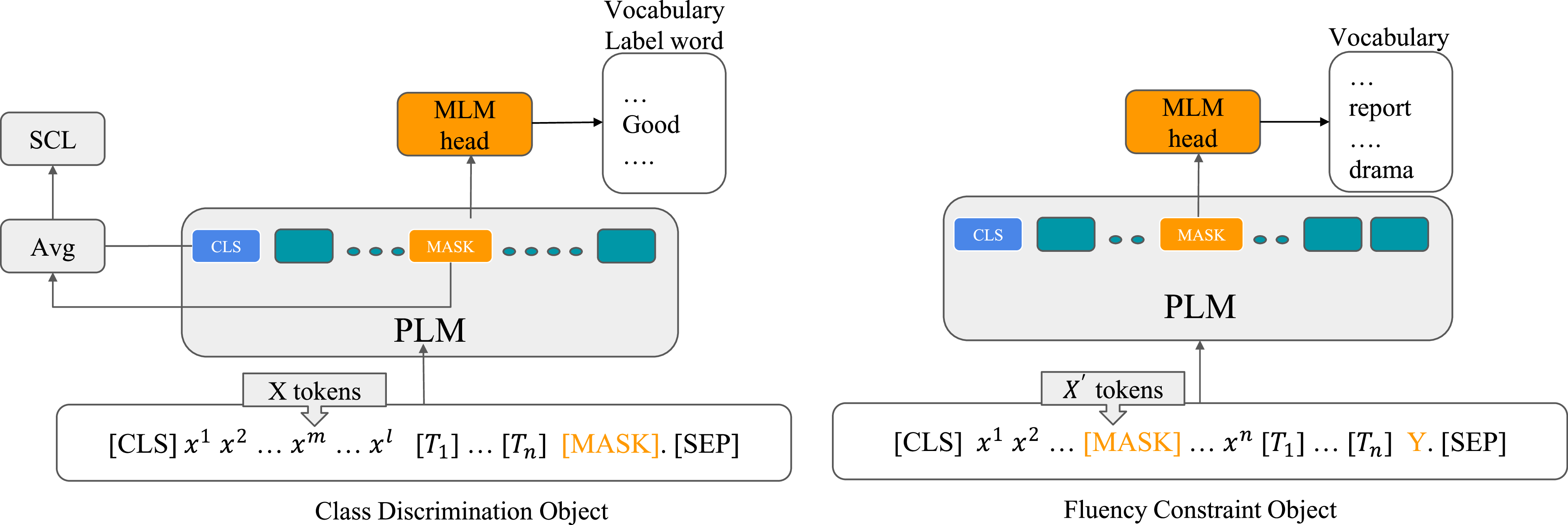
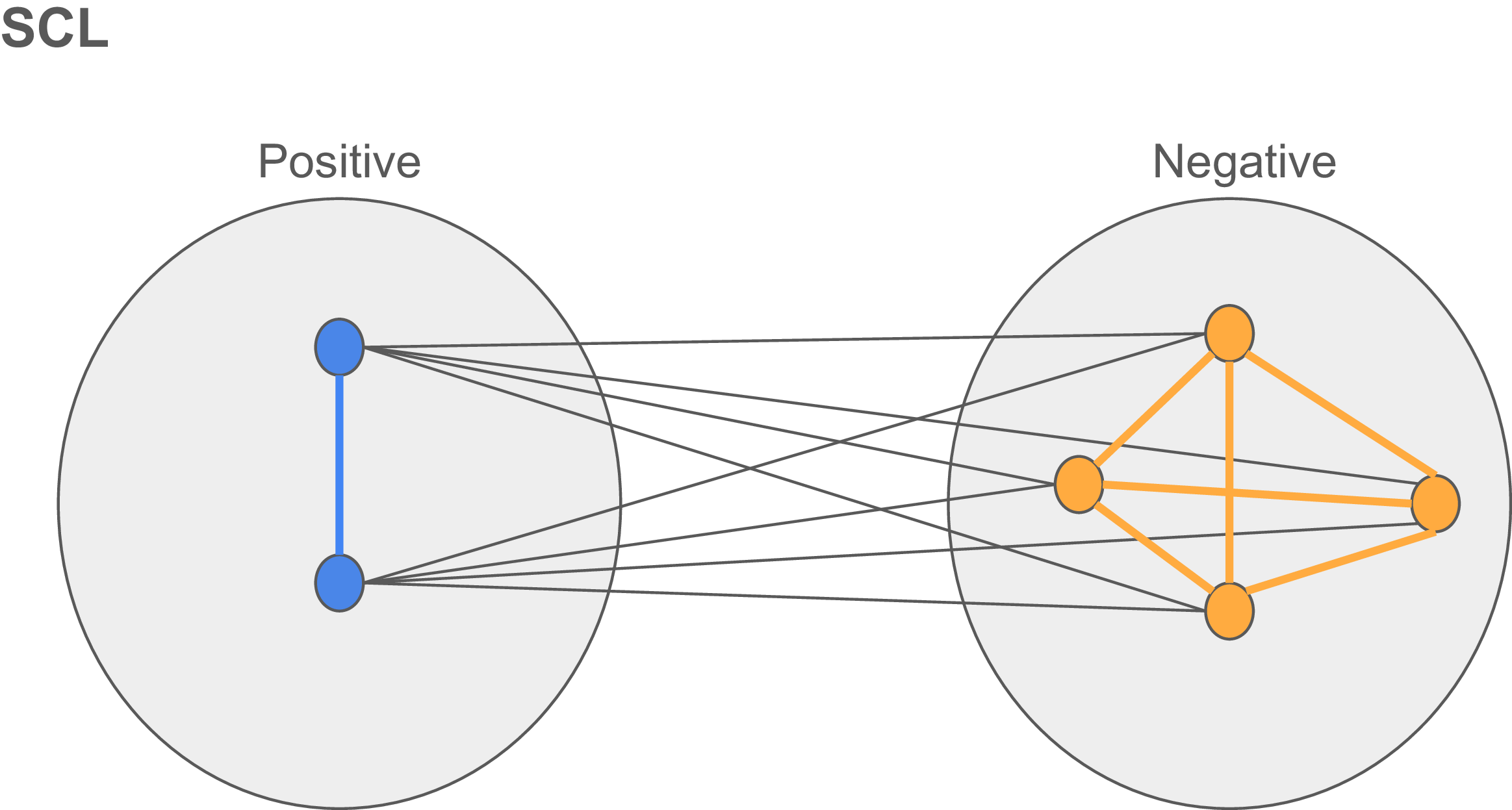

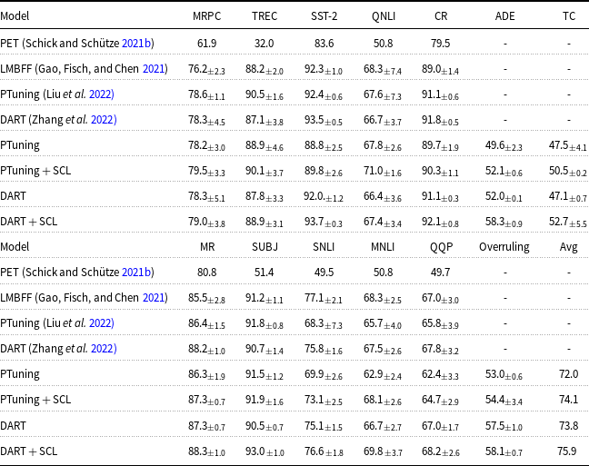
 ±
±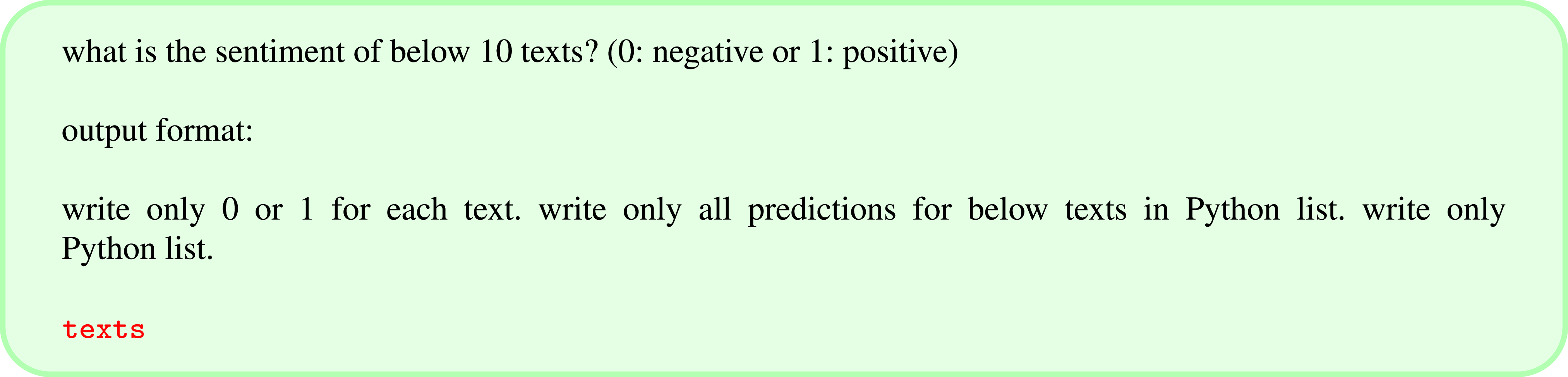
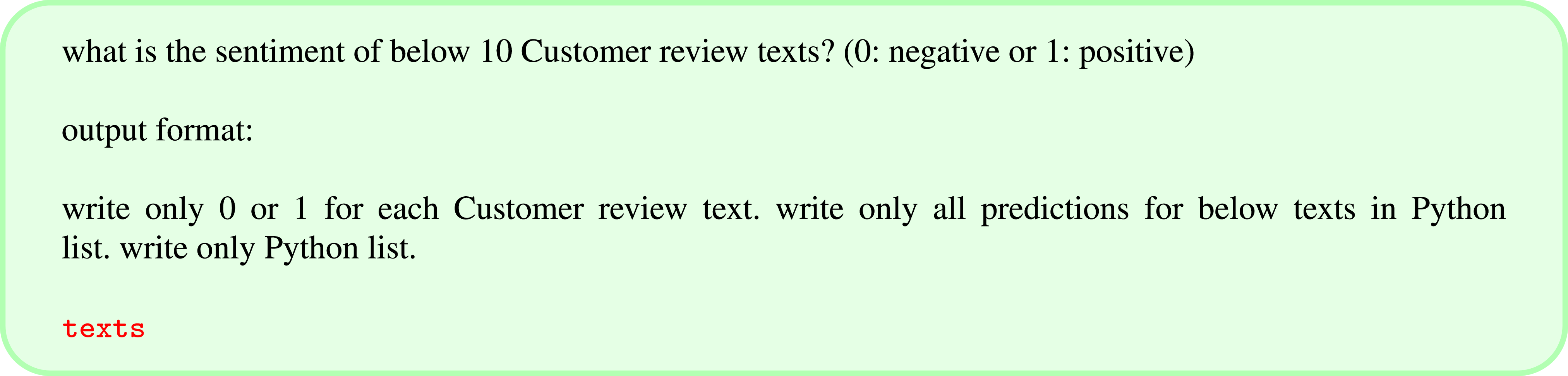
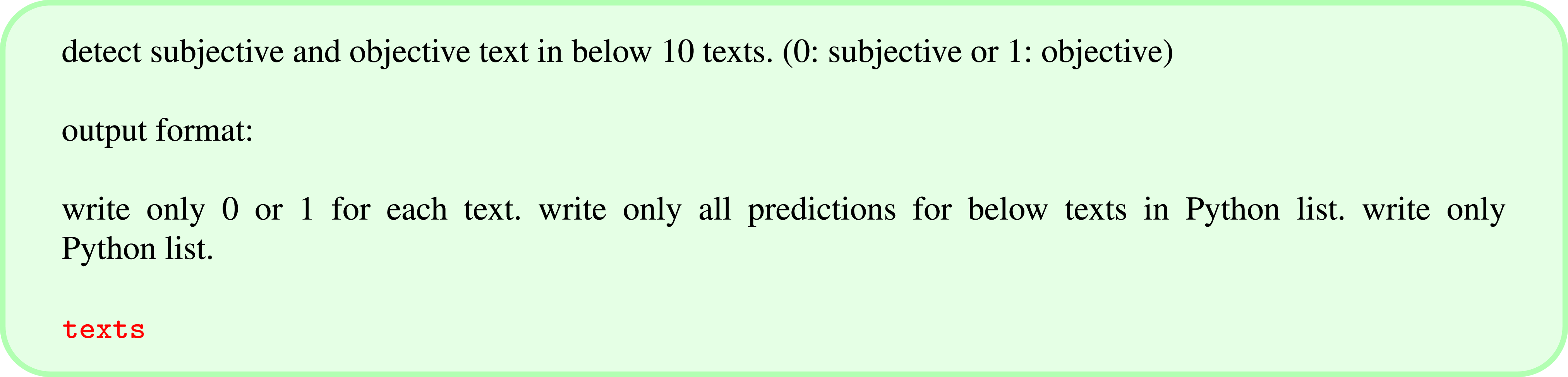
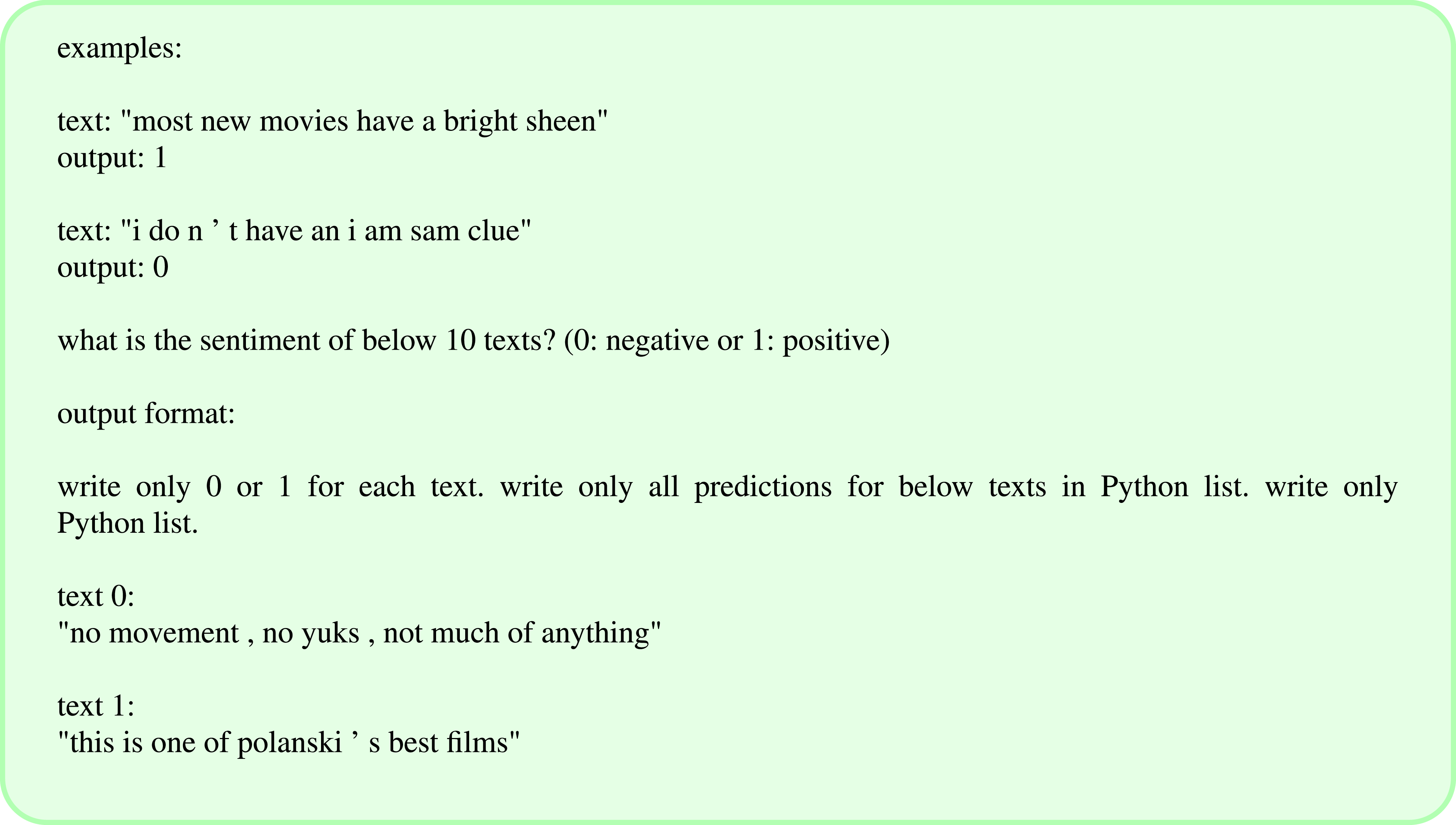
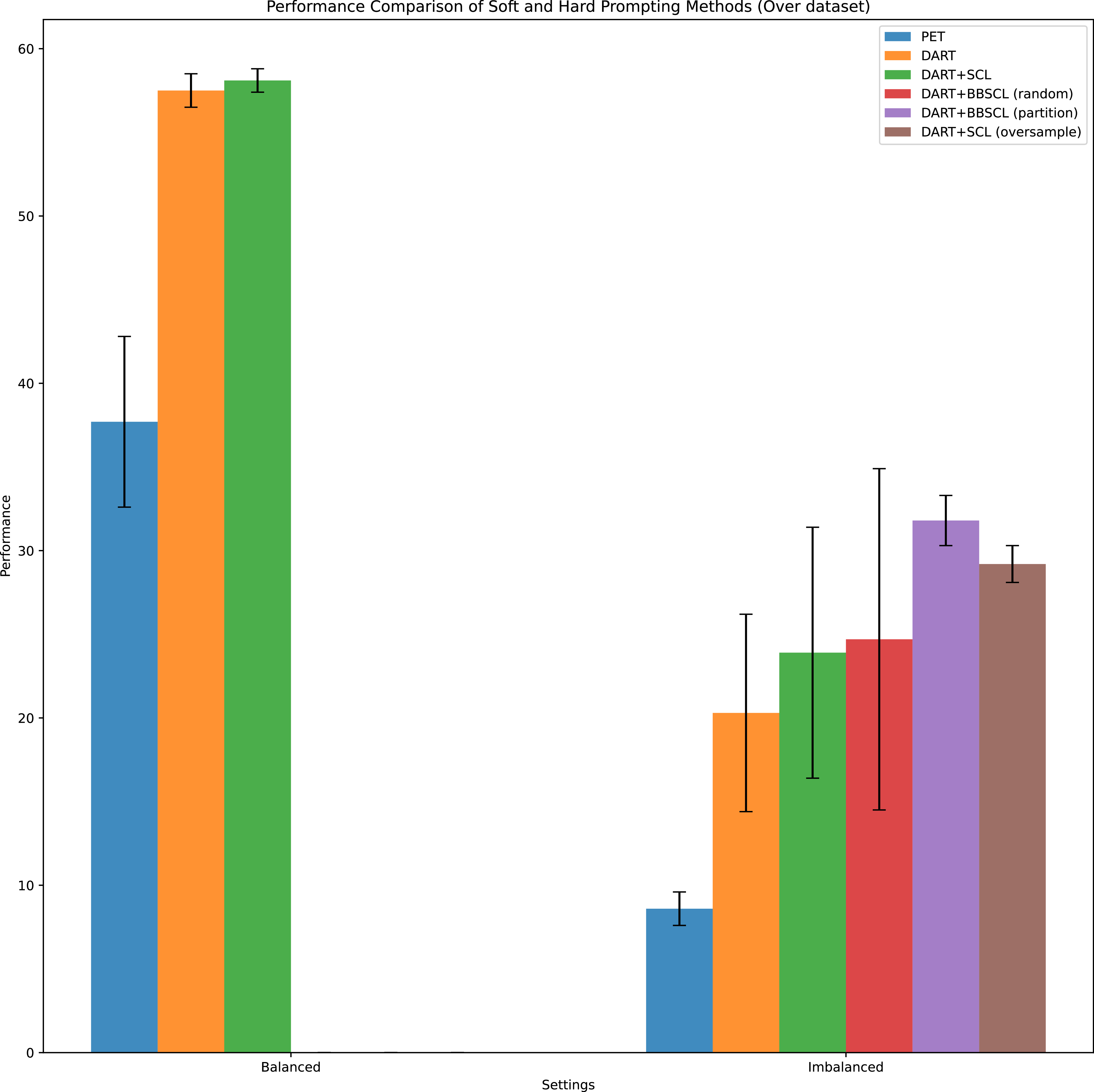
 ±
± ρ
ρ ρ+=0.25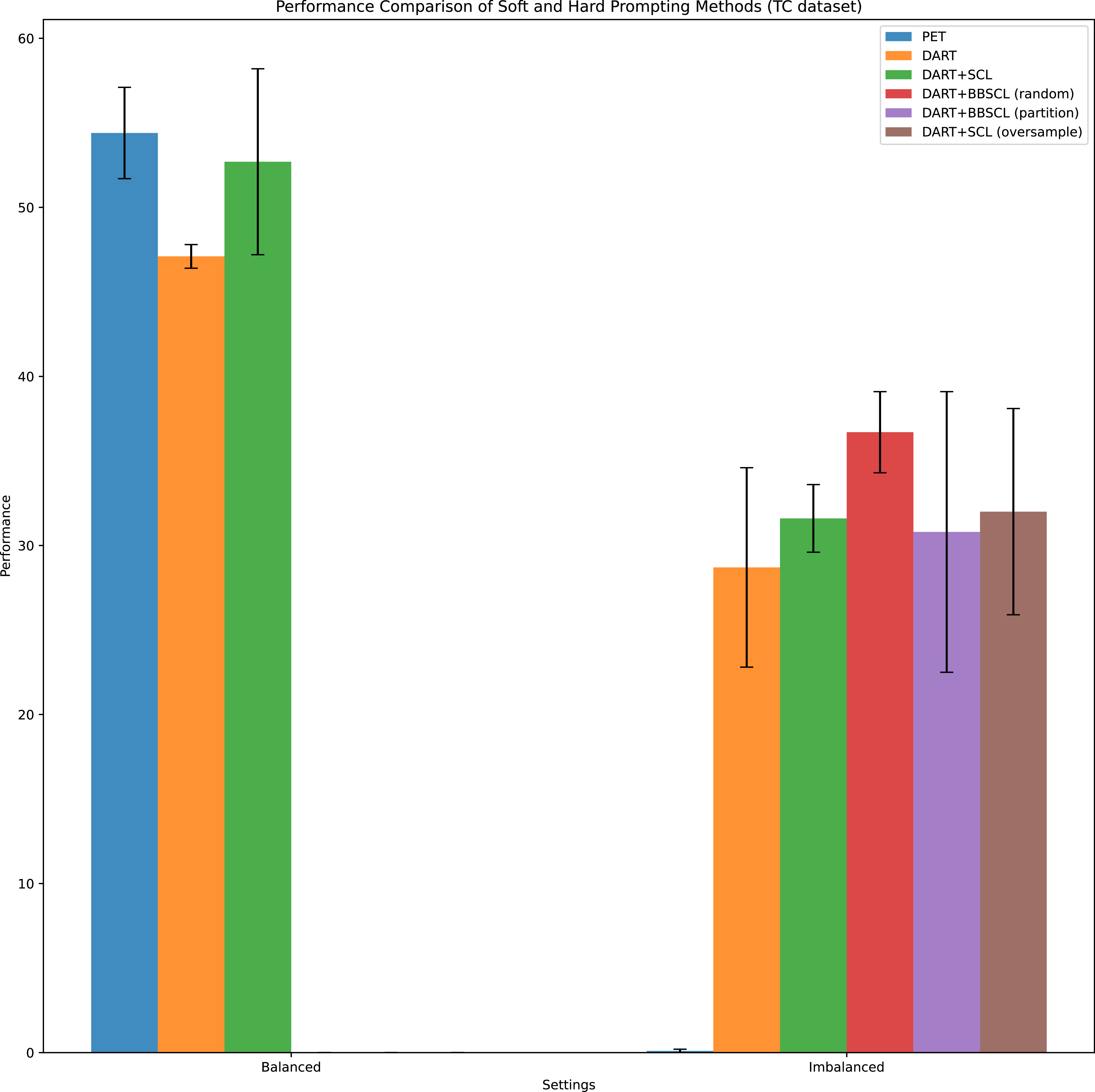
 ±
± ρ
ρ ρ+=0.25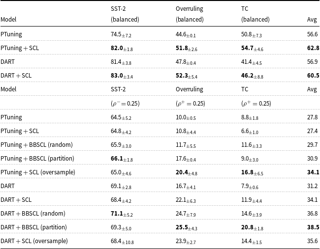
 ρ
ρ posall=ρ+
 negall=ρ−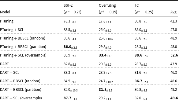
 ρ
ρ posall=ρ+
 negall=ρ−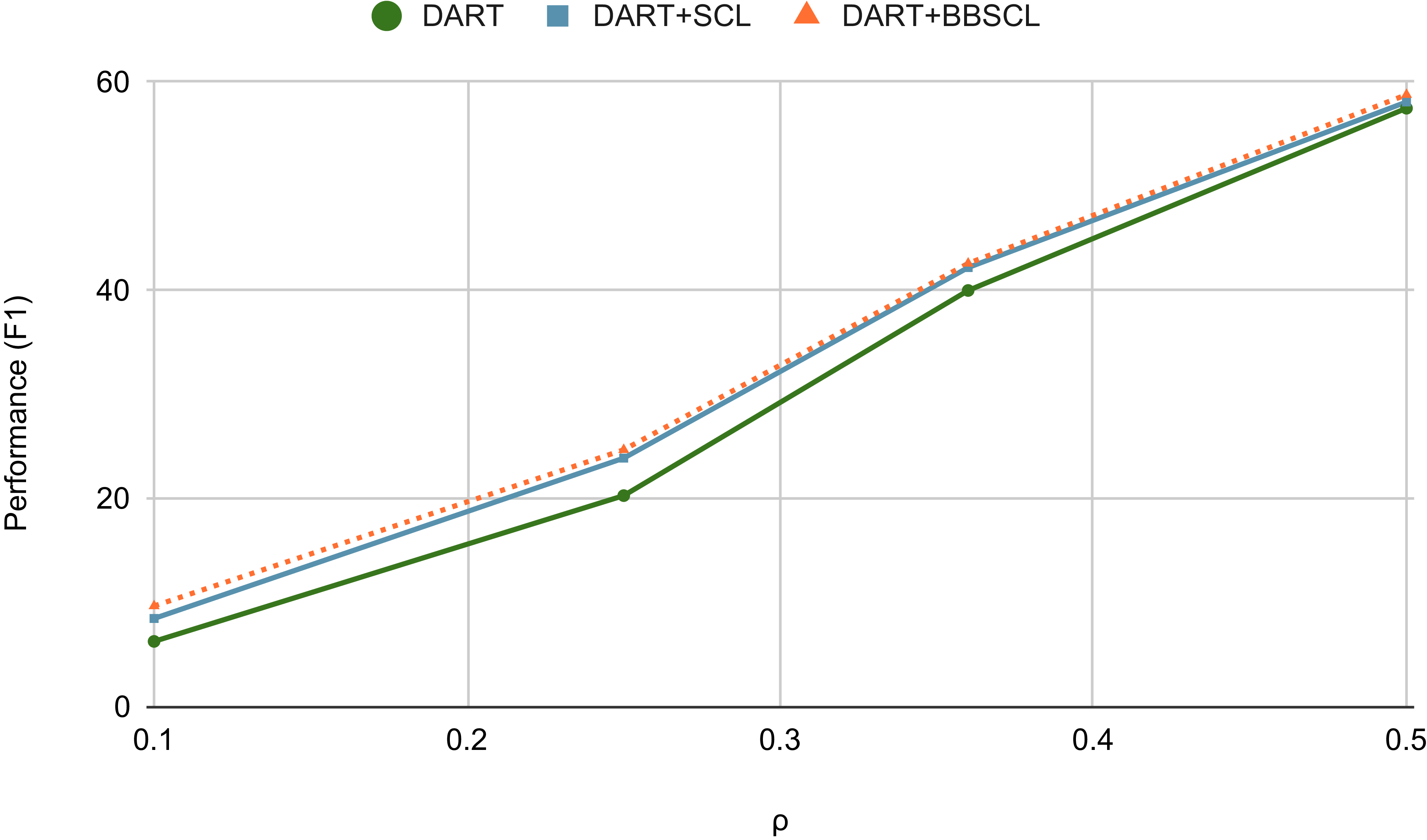
 ρ+={0.1,0.25,0.36,0.5}
 ρ+=0.5
 ρ+
ρ+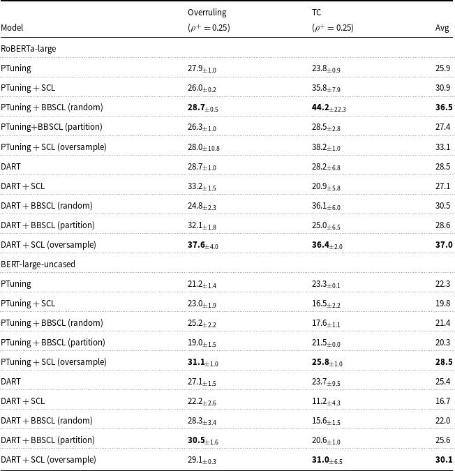
 ±
± ρ
ρ posall=ρ+
 negall=ρ−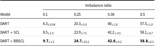
 ρ+={0.1,0.25,0.36,0.5}
 ρ+=0.5
 ρ+
ρ+
 RD=0.44
 RD=0.84
 RD=0.85
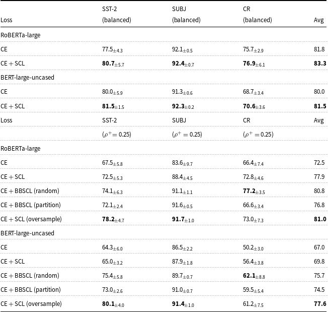
 ±
± ρ
ρ posall=ρ+
 negall=ρ−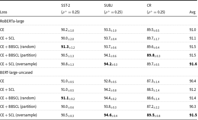
 ±
± ρ
ρ posall=ρ+
 negall=ρ−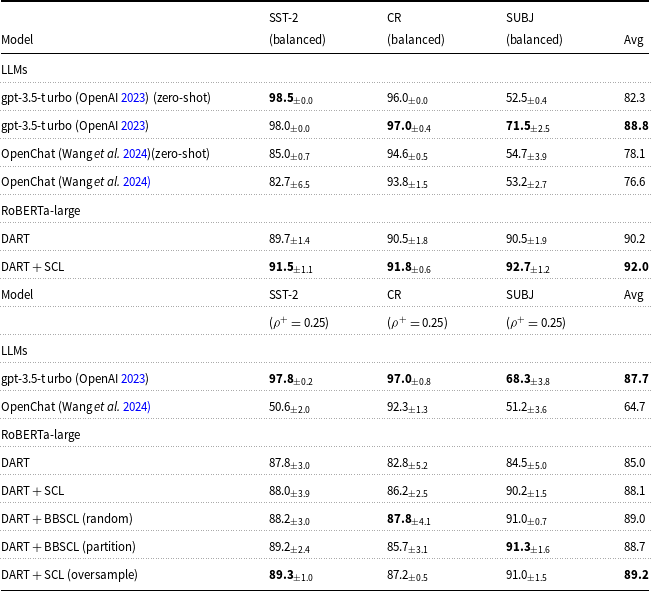
 ±
± ρ
ρ posall=ρ+
 negall=ρ−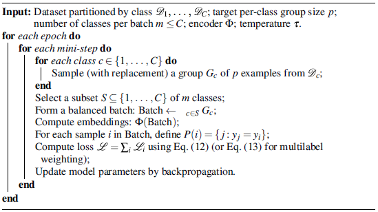
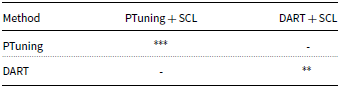
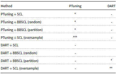
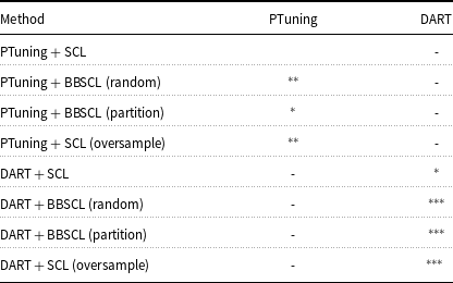
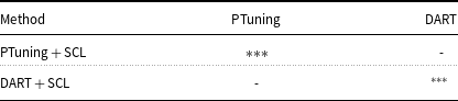
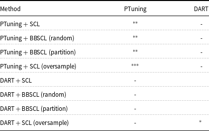
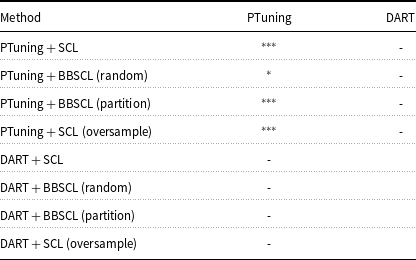
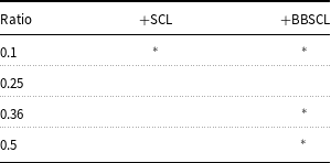

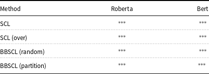
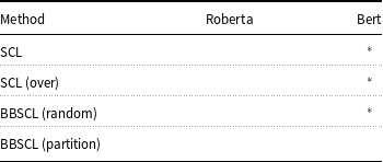
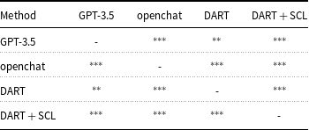
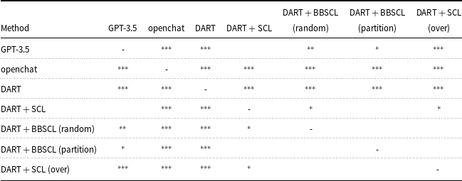


 Open access

