A p-Value May Not Be Telling You What You Think It Is

The definition of a p-value is innocuous enough: it is the probability of observing a statistic or one more extreme if the null hypothesis is true. In other words, we assume that the null hypothesis is true, and based on that assumption, we calculate the probability we would observe our statistic or a more unusual or extreme value. If that probability is small relative to what we choose as our significance level (typically but not necessarily 0.05), we reject the null hypothesis. If that probability is large, we accept the null.

It is important to realize that we never prove that the null hypothesis is true or that it is false; that is impossible, because the p-value tells us that there is some probability that our statistic could have arisen if the null was true. For example, the probability of drawing a flush (five cards all of the same suit) in a game of poker is 0.00198, far less than 0.05, but drawing one does not prove that the deck is stacked. All that we can do is use statistical inference to decide how to proceed. By rejecting the null hypothesis, we will act as if it is false, knowing full well that it might be true, in which case we have made a type I error. If we accept the null hypothesis, we will act as if it is true, being aware that we have made a type II error if the hypothesis is actually false.

It is common to hear people state that a p-value is the probability that your null hypothesis is true, but it is not. A simple analogy shows why. Suppose you tally the color of frogs and find that 75% of frogs are green. You could then say, “If it is a frog, there is a 0.75 probability that it is green.” Note that this statement is in the same form as the definition of a null hypothesis: if X, then there is a probability of Y. You cannot invert this to say, “If it is green, there is a 0.75 probability that it is a frog,” because if you find something green in nature, it is far more probable that it is a plant or an insect! Inverting the definition is a logical fallacy called affirming the consequent.

In short, p-values do not tell if the null hypothesis is true or false, nor do they give a probability that the null is true.

Smaller p-Values May Not Mean That You Have Found an Important Pattern

R. A. Fisher (Reference Fisher1925) introduced the term “statistically significant” to describe any outcome that was sufficiently rare to suggest that further investigation was warranted, and he chose 1/20 (0.05) as sufficiently rare. He did not argue that there was something intrinsically special about a 0.05 standard, or that achieving this standard was noteworthy in any sense other than that it was unusual enough to suggest further investigation of the pattern. “Statistical significance,” often shortened to “significance,” was a poor choice of wording on Fisher's part, because significance to most people implies importance, and statistically significant results are not necessarily scientifically important ones.

When we think of a finding as important, we think of one that is substantially different from what we expected, that is, our null hypothesis. It could be a correlation coefficient that is much closer to positive or negative one than the null hypothesis of zero, or a difference in means that is much larger than the null expectation of zero. When “statistically significant” is shortened to “significant,” it is easily misconstrued as meaning that the result is quite different from the null expectation. Describing small p-values as “highly significant” compounds this problem. I advise my students to mentally substitute “nonzero” when they read the phrase “statistically significant” or “significant,” as it clarifies what the statistical test established and how remarkably little it tells us.

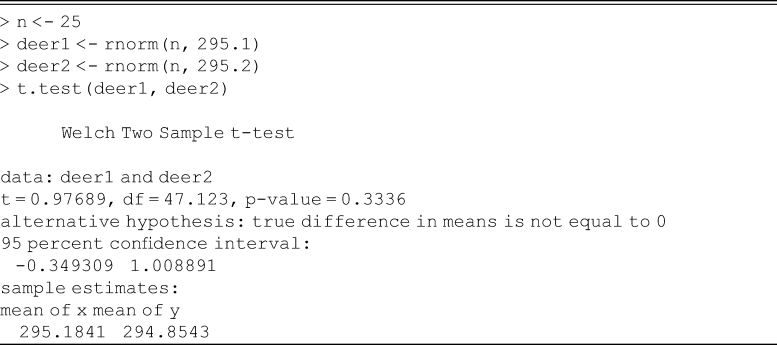
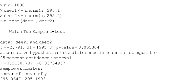
Although we intuitively anticipate a small p-value when our results are substantially different from the null expectation, small p-values can just as easily arise because our sample size is large. A simple example helps demonstrate this. For example, suppose the adult femur lengths of two populations of deer differ by a small amount. This difference is known as effect size, and it is what we would most like to know. If we gather a small amount of data, say 25 individuals from each population, and perform a t-test on the difference in means, we will probably obtain a large p-value, that is, a statistically nonsignificant (>0.05) value (Table 1). This seems intuitive: the difference in means is small, and we would expect the p-value to not be statistically significant. However, if we gather a large amount of data from these same populations, say 1000 individuals of each, the results of our t-test now reveal a significant p-value (Table 2). If we increased the sample size even more, an even smaller p-value would result, eventually one so small that one might describe the outcome as highly significant. The difference in femur lengths has not changed at all, the effect size is the same throughout, and the difference in means is no more important in the large data set than the smaller one. The only reason for the increasingly smaller p-values was the ever-growing sample size, which eventually allowed us to detect a tiny departure from the null hypothesis. Often, statistically significant results are such small departures from the null that they are not scientifically important (see Ranstam [2012] for a good demonstration using clinical medical trials).

Table 1.

Simple R simulation showing the statistically nonsignificant difference in the mean adult femur lengths of two deer populations. These results are representative; repeating this process 1 million times indicates that the null will correctly be rejected (i.e., statistical power) only 6.3% of the time at α = 0.05, 1.4% of the time at α = 0.01, and 0.2% of the time at α = 0.001. Most of the time, such a small difference in means would not be successfully detected at this small sample size.

Table 2.

Simple R simulation showing that the difference in the mean adult femur lengths of the same two deer populations shown in Table 1 are statistically significant when sample size is large. These results are representative; repeating this process 1 million times indicates that the null will correctly be rejected (i.e., statistical power) 60.9% of the time at α = 0.05, 36.7% of the time at α = 0.01, and 14.5% of the time at α = 0.001. This small difference in means will be successfully detected far more often when n = 1000 than when n = 25 (Table 1).

Because p-values are controlled by effect size, sample size, and variance, simply tagging results with adjectives like “significant” or “highly significant” is misleading. It is not the p-value that makes the result important (or significant, in everyday language), it is the effect size (Sullivan and Feinn Reference Sullivan and Feinn2012). It is not uncommon to find statistical results reported as a table of p-values, with no mention of effect sizes, which completely obscures what we need to know to understand whether what has been found is an important relationship.

Most Significance Tests Serve No Purpose

In most cases, the null hypothesis states that the effect size is zero, such as a difference in means of zero or a correlation of zero. Because p-values are partly controlled by sample size, it becomes increasingly possible to detect ever-smaller effect sizes with large-enough data sets. In other words, given that some nonzero effect size exists, obtaining a statistically significant result is only a matter of collecting enough data. This becomes a greater problem as enormous data sets become available. Modeling studies are particularly subject to spuriously low p-values because the number of replicates can be set as high as computing time allows (White et al. Reference White, Rassweiler, Samhouri, Stier and White2014).

In many cases, significance testing with a p-value is the wrong approach, because the null hypothesis can often be rejected before a single piece of data is collected. For example, consider those two populations of deer. If we reflect on the null hypothesis, that the difference in mean adult femur lengths is zero, we know that we should reject the null hypothesis before we even begin to collect the data (Johnson Reference Johnson1999).

How can we say this? Imagine precisely measuring every single adult deer femur in those two populations. Those means are almost assuredly different; the difference in means might lie in the fourth or fifth decimal place, but the probability that those two deer populations have exactly the same mean adult femur length is vanishingly small. Gaining a statistically significant result is only a question of collecting enough data. A statistically insignificant result most likely indicates only that we have not collected enough data. The statistical test is not telling us anything useful, and that is true for a great many tests. Using MANOVA to test for differences in community composition or ANOVA to test for differences among groups are two common examples.

Confidence Intervals Are More Informative

Our original goal in running statistical tests was to convince ourselves that the patterns in the data are real, that they did not arise from random chance when the null hypothesis is true. Simply throwing out significance testing and p-values will not solve our problem, because it leaves our original goal unsatisfied. Confidence intervals are one way to address our original goals while avoiding the problems of p-values and significance testing (Gardner and Altman Reference Gardner and Altman1986; Yoccoz Reference Yoccoz1991; Rigby Reference Rigby1999; Ranstam Reference Ranstam2012; Cumming Reference Cumming2014).

I showed earlier how, with enough data, we could reject the null hypothesis for any effect size, no matter how small. Many of those small effect sizes might be biologically unimportant for many questions, and whether an effect size is meaningful will depend on the particular problem (Houle et al. Reference Houle, Pélabon, Wagner and Hansen2011). For example, a difference in mean adult femur length of 0.01 mm is likely to be biologically unimportant for many questions, but a difference in speciation rates of 0.01 per lineage Myr could have a substantial effect. In the deer example, the null hypothesis addresses only a difference of 0.0 mm, and it would be good if we could also test (and reject) all of those other biologically unimportant hypotheses. Confidence intervals do just that, because a confidence interval is the set of all acceptable hypotheses. For example, if we have confidence limits of 5.7–10.3 mm, we can reject every hypothesis that lies outside those limits at that level of confidence. This accomplishes what our single p-value did, and much more.

When our confidence interval is expressed in the form of E ± U, it provides us with two useful pieces of information. First, it provides an estimate of effect size (E), the quantity that tells us directly how important our result is, such as how strong the correlation is, what the slope is between two variables, or what the difference of means is between two populations. Second, it provides an estimate of uncertainty (U) in our results, one that allows us to test not only an often manifestly false null hypothesis but also a large set of alternative hypotheses. This estimate and uncertainty can be used in subsequent models, allowing us to propagate our understanding (effect size) and our uncertainty forward through other studies. Confidence intervals decrease with sample size, reflecting our greater certainty in our estimate as we collect more data.

Bayesian credible intervals perform a similar function of providing an estimate and an uncertainty. For many types of problems, Bayesian credible intervals and frequentist confidence intervals give comparable results (Bolker Reference Bolker2008; Wang Reference Wang2010).

Significance Tests May Ask the Wrong Question

After Eldredge and Gould (Reference Eldredge, Gould and Schopf1972) introduced their hypothesis of punctuated equilibria, paleobiologists undertook a concerted effort at documenting patterns of morphological evolution, especially testing the existence of stasis in the geological record. It was soon realized that morphology might appear to show directional change over time, even though morphology was undergoing only a random walk (Raup Reference Raup and Hallam1977; Raup and Crick Reference Raup and Crick1981). It was soon realized that statistically rejecting a random walk was exceptionally difficult (Bookstein Reference Bookstein1987; Sheets and Mitchell Reference Sheets and Mitchell2001).

Progress on this question was hindered until it was realized that testing a single hypothesis, the null, was the wrong approach, that the question should not be whether a null can be rejected, but which model of evolution (random drift, directional, punctuated, etc.) was best supported by the data. Applying likelihood-based model selection to a wide variety of taxa, Gene Hunt (Reference Hunt2007) showed that random walks and stasis in morphology were equally frequent, and that directional change was far less common. Expanding on this approach, Hunt (Reference Hunt2008) used likelihood-based model selection to distinguish between gradual and pulsed evolution and to estimate the underlying parameters that describe the morphological history. The advantage of using information criteria in these types of studies is that they incorporate penalties for more complicated models, making it difficult to overfit the data with a too-complicated model and thereby appealing to Occam's razor. Model selection achieves a similar end as estimation, in that the goal is not to test a single hypothesis (the null), but to evaluate a range of hypotheses to understand which is best supported by the data. It is also important to bear in mind that a selected model may not fit the data well, and that models not considered may fit the data considerably better (Pennell et al. Reference Pennell, FitzJohn, Cornwell and Harmon2015; Voje et al. Reference Voje, Starrfelt and Liow2018).

A Path Forward

Fortunately, it is straightforward to move beyond significance testing and p-values. Most simple tests in R (R Core Team 2018), such as those for proportions, means, variance, correlation, and regression, automatically report confidence intervals. Adopting them is only a matter of reporting a different line in the output. Bayesian credible intervals have been more difficult to calculate, and their methods less standardized, but that situation is steadily improving. Methods of model selection are also less standardized, but a growing number of implementations make the barrier to incorporating them ever lower.

Instead of performing significance tests, we should estimate parameters and the uncertainty in those estimates. Rather than aiming for small p-values, our goal should be effect sizes that show that we have identified important relationships, along with uncertainties reduced through larger sample sizes.