

Introduction
The Baltic Sea is located in the seasonal sea-ice zone, and winter navigation in the Baltic Sea is very important for the economy of the area. To enable efficient winter navigation, operational ice monitoring and ice forecasting based on numerical ice models are required. The maximum annual ice extent, typically reached in February–March, is 10–100% of the Baltic Sea area (400 000 km2). The Baltic ice season lasts 4–7 months, and the maximum annual thickness of landfast ice is 50–120 cm. Freezing begins in the northern parts of the Gulf of Bothnia between mid-November and December. Interannual variation between ice seasons can be large (Reference Leppäranta and SeinaLeppäranta and Seina, 1985). The ice season evolution is driven by the weather, ice/water interactions and the icefield internal processes. In the shallow coastal areas, landfast ice develops relatively rapidly and it remains relatively static until the melt season. A map of the Baltic Sea fast-ice areas, based on the detected synthetic aperture radar (SAR) motion during winter 2010/11, is shown in Figure 1. The ice concentration in these areas is very high, close to 100%. In the white areas of the figure it is typically <100%; in these areas the ice is moving and deforming mainly due to variable wind conditions.
Ice areas with no ice motion (black) during a 4 week period (February 2011) in the Baltic Sea according to SAR data. These areas correspond to the typical fast-ice areas in the Baltic Sea. They typically have ice motion only during the early winter (very thin ice easily broken by waves) and late winter (late melting season, when the ice starts to break).
Monitoring of ice motion based on coastal radars has been studied and found useful in multiple cases (e.g. Reference Wakatsuchi and OhshimaWakatsuchi and Ohshima, 1990; Reference Shevchenko, Rabinovich and ThomsonShevchenko and others, 2004; Reference Mahoney, Eicken and ShapiroMahoney and others, 2007; Reference Druckenmiller, Eicken, Johnson, Pringle and WilliamsDruckenmiller and others, 2009). Automated ice motion estimation based on coastal and ship radars has been studied at the Finnish Meteorological Institute (FMI) for some years. Previously we have developed an algorithm (Reference KarvonenKarvonen, 2012) for detecting ice motion from spaceborne SAR data. The same algorithm with different parameters can also be applied to define ice motion fields for the radar data (Reference Karvonen, Heiler and HaapalaKarvonen and others, 2010). Here we have developed an algorithm, based on a similar technique, to track the drift of ice objects located in the first image of an image sequence. The traceable ice objects are located by a detecting algorithm before tracking. After detecting the initial objects, they are tracked to the end of a tracking period, or until the object can no longer be located by the algorithm. The algorithm is based on locating the maximal phase correlation between two image windows, sampled from two successive radar images of a radar image time series around given center points, corresponding to the located objects. The algorithm is performed in two resolutions for each traceable object: first, the coarse drift is estimated in a lower resolution, then it is refined in a high (full-image) resolution. The algorithm also takes into account the rotation of the features, by rotating another of the two image data inputs in the correlation maximum search. The main difference compared to our ice-drift algorithm (Reference Karvonen, Heiler and HaapalaKarvonen and others, 2010; Reference KarvonenKarvonen, 2012) is that in this new ice-tracking algorithm we first locate candidates for the traceable objects, and then track these objects to the end of the tracking period or until they are not reliably recognized by the algorithm. In our ice-drift algorithm we compute the ice drift for each gridpoint between two adjacent images, if a quality measure exceeds a given threshold. If the quality criteria are not satisfied, no ice-drift estimate for the gridpoint is given. In the ice-drift algorithm we also apply a spatial filtering, taking into account the motion in the neighboring gridcells, to yield coherent motion fields. In the new tracking algorithm the objects to be tracked are automatically selected in such a way that they can be tracked reliably without taking the neighborhood into account. This makes the selection of the objects a crucial step of the algorithm.
We have tested the method for some radar image time series with a 10 min temporal spacing. The results for the studied time series were encouraging and corresponded to our visual interpretation relatively well. In this paper, we show two ice-tracking cases and also present analysis and discussion of the tracking results.
The multi-category sea-ice model HELMI (HELsinki Multicategory Ice model) (Reference HaapalaHaapala, 2000; Reference Haapala, Lönnroth and StösselHaapala and others, 2005) has been in operational use at FMI for several ice seasons. An implementation of a finer-scale (closer to ship-scale) version of the model has also been studied as part of the European Commission (EC) FP-7 SAFEWIN (Safety of Winter Navigation in Dynamic Ice) project. Our aim is to utilize the developed tracking algorithm to validate the fine-scale HELMI model. Computation of the validation data will be automated as far as possible. The idea is to locate and track objects continuously until most of them are no longer reliably recognized by the algorithm, and then start the tracking again with new objects located in a new initial image. To maintain continuity, there should be some temporal overlap between two temporally adjacent tracking time series.
Radar Image Capturing and Preprocessing
The radar image capturing unit (radar video server) used by FMI has been developed by a Finnish company, Image Soft Ltd. The radar video server has a 20 MHz sampling rate. It is based on PC technology and forms PPI (plan position indicator) images from the radar signal, the triggering pulse and the antenna pulse. PPI is the most common type of radar display. The radar antenna is represented at the center of the display, so the distance from it and height above ground can be drawn as concentric circles. The received radar signal contains information on the echo intensities and distances. Triggering and antenna pulses indicate when and in which direction the radar signal was sent. The azimuth change pulse (ACP) is a pulse set between a fixed angle in radar rotation. Typically there are 2n pulses per 360°. The azimuth reset pulse (ARP) is a reference pulse set at a reference point. The radar angle is derived by counting the number of ACPs since the most recent ARP. The images are constructed based on these pulses and on the recorded echoes with a known time difference.
For the two coastal radars currently used by FMI, the total area imaged is 40 km × 40 km, and the image size is 1200 × 1200 pixels, resulting in a nominal resolution of 33 m. Naturally the true resolution depends on the radar parameters, and in the far range the resolution is restricted by the angular (or bearing) resolution. The image origin, i.e. location of the radar, is shifted such that the origin of our radar images is located at (30 000 m, 20 000 m) from the upper left corner of the images, i.e. the origin has been shifted to the east by 10 km. This was done because the two coastal radars are located on the eastern side of the Gulf of Bothnia, and after this shift we can see more sea area in the images. The Tankar coastal radar images are additionally rotated clockwise by 50° due to the shape of the coast at the location. After this rotation the Tankar radar images cover less land area, and the ship lead to Kokkola harbor is better covered.
A temporal median filtering is applied to the image data, using nine first images for each whole minute (e.g. corresponding to 9 s if the radar rotates 60 rounds min - 1). This filtering reduces the radar imaging noise and effectively filters some other undesired random effects (radar artifacts). In our experiments we use a 10 min time interval between each image pair of an image time series, i.e. we use temporally down-sampled data. For the two cases presented here, we have not applied any other filtering. However, we also present some candidates for filtering techniques to improve the tracking reliability.
Locating the Traceable Ice Objects
The traceable objects are objects that can reliably be traced from one image to another. The first condition for a traceable object is that there exist some features (texture) at the location, thus excluding even surface areas shown as white noise by a radar. To take this condition into account, we have included the local image pixel value standard deviation as one criterion for a traceable object. Secondly, we require a traceable object to contain corner points, because we want an object to include corners or curved edges, not only straight edges. Straight edges are problematic for tracking because the image often looks very similar along a straight edge, and similarization errors made by correlation-based algorithms may occur along straight-edge lines. The objects to be tracked are determined based on features computed within a radius R from the center point; the row and column coordinates of the point are denoted by (r, c) here. The local texture in an image can be characterized by the local image pixel standard deviation σ(r, c) computed as

where μ is the local image pixel value mean computed as
I(i, j) is the image pixel value at (i, j), and N is the number of pixels within the radius R. Additionally we can require that an object contains a strong edge content, i.e. there are many edge points within the object, indicating an ice type edge or some kind of ice deformation pattern (e.g. a ridge). This condition complements the requirement of high σ(r, c).
We first define a regular uniform grid with uniform spacing in both the row and column directions, and around each gridpoint we find one point within a given radius R g from the gridpoint, maximizing the value of an energy function E(r, c), with respect to (r, c). E(r, c) is given by
or
where σ(r, c, R) is the local image pixel value standard deviation computed within the radius R from (r,c), and N c and N e are the numbers of corner and edge points, within the radius R from (r, c), respectively. We use a product form because we want both or all three terms to have a high value for a traceable object. Both versions of E(r, c) produce similar results. The corner points are computed using two algorithms, and all the points produced by either algorithm are included as edges. The first algorithm is the Harris corner detector (Reference Harris and StephensHarris and Stephens, 1988), and the other is based on local binary patterns (LBP; Reference Ojala, Pietikäinen and HarwoodOjala and others, 1996). The edges are located by the same algorithms as the corners; a corner pixel is just a special case of a detected edge pixel (Fig. 2). An example of the edge detection is shown in Figure 3. After detecting the edges, we remove small edge segments, i.e. edge segments of fewer than T e connected edge pixels. A typical threshold value is T e = 5. This filtering reduces the number of edges produced by imaging noise.
An example of a straight edge line (upper) and a curved edge line (lower); the edge pixels appear as black. Sharp corners are corners sharper than 90°. At pixel level a curved edge always contains corner points; this is also true for smoothly curved edge lines, because at pixel level they are quantized to pixels. All the corner points are also edge pixels.
An example of the edge detection for a selected part of a radar image (25 February 2011): the radar image (left) and the edges (black tone, right). The origin is located at the right side of the image in the middle.
In this version, the LBPs are formed such that a threshold, T, for the absolute difference between the middle point and the reference points is applied; here we use T = 10. The reference points are the eight points with the angular step of Π/4 around the middle point within a given distance R LBP; here we use R LBP = 2. After computing the local binary pattern for each pixel location, the minimum of all the cyclic shifts of the eight-bit number is selected as the LBP for the pixel. This operation makes the values rotationally invariant. These LBP values can then be interpreted as edges (LBP value 15), corners (31) and sharp corners (63). We also recognize the LBP values of 31 and 63 as corner points, i.e. allowing one-bit deviation in the LBP.
Tracking Algorithm
The tracking is performed for each pair of successive radar images of a radar image sequence, which here is a radar image time series with a constant temporal sampling rate. The object locations in the first image of the image pair are known (either based on the the initial object detection from the first image or as a result of the tracking for later images). The algorithm is based on phase correlation between the two image windows around the centers of the objects. The phase correlation is computed in two resolutions for each object. First, candidates for the motion are defined in a coarse resolution, then the final motion estimate is defined in a fine scale. Some multi-resolution phase-correlation algorithms for sea-ice drift estimation between SAR image pairs have been developed previously (e.g. Reference Thomas, Geiger and KambhamettuThomas and others, 2004; Reference KarvonenKarvonen, 2012). In a tracking algorithm the computation is performed for the located objects only, and because the number of objects is restricted, computation is much faster than computing the motion for a whole common area of two images. The objects are also selected in such a way that they can reliably be traced, reducing the possibility of confusion (similarization errors) associated with correlation-based algorithms.
The regular image window size is W × W; we have used W = 16. This image size was selected experimentally. Two factors restrict the size of the window: the fast Fourier transform (FFT) used in the computations requires the size to be a power of two, and the window must contain enough information for reliable tracking. On the other hand, selecting a larger window size than necessary reduces the spatial resolution (traceable objects become larger). To compute the phase correlation, the two-dimensional FFT (2D FFT) is applied to the data windows sampled from the two images around the object location (in the first image, where it is known). Then FFT coefficients of the two image windows are normalized by their magnitudes, the FFT coefficients of the two image windows are multiplied by each other and the inverse 2-D FFT is applied. The phase correlation array is also computed from the the normalized cross power spectrum. The best matching displacement in a Cartesian (x, y) coordinate system is defined by the maximum of the phase correlation, here denoted by PC:
Because the FFT assumes the data are periodic, a Gaussian window is applied to the data windows before the transformation. The drift is estimated in the row–column (r, c) coordinate system in whole pixels at two resolutions, i.e here we make a replacement: x → r, y → c. The displacement vector in the row and column coordinates is denoted by (dr, dc). In practice there often occur several correlation maxima which can be close to each other, and it is reasonable to use more than just one drift candidate for one window pair, and make the final decision only at the fine-resolution level.
For the low resolution, the two images are first down-sampled to a given resolution. Because the FFT is used, the down-sampling rate R S should be a power of two, i.e. R S = 2n– 1; we have used n = 3, corresponding to R S = 4, which is an adequate value for 10 min radar motion. The two low-resolution images are generated by successively applying a half-band low-pass finite impulse response filter designed for multi-resolution image processing (Reference Aiazzi, Alparone, Baronti and BorriAiazzi and others, 1998).
After down-sampling to the low resolution, we go through objects in the first image, and for each object location we make the two W × W sample windows and find the correlation maxima. At the low resolution the phase correlation for each object is also computed for rotated windows, such that the data windows sampled from the first image, in which the object is centered, are rotated between –15° and +15° in steps of 5°. This also allows the cases of slight object rotation, assuming the rotation for the selected time interval is between –15° and +15°. The M maximum correlations among all seven orientations, the corresponding motion coordinates (dr L,dc L) and rotation are stored. These values are here called low-resolution drift candidates. We use the parameter value M = 12. If the zero-motion case (dr, dc) = (0, 0) is not included in the M low-resolution drift values indicated by the maxima, it is included and the low-resolution drift candidate with the lowest phase correlation is excluded. This list of M drift candidates, corresponding phase correlations and rotation angles for each object location is then delivered to the fine-resolution processing. At the fine-resolution level, all the displacements from the low-resolution level, scaled up by the down-sampling rate R S, are considered as potential low-resolution ice-drift candidates. All the low-resolution drift candidates are gone through by sampling the image windows around the object locations in the first image, and around the corresponding first-image locations shifted by the low-resolution shift and scaled by R S in the second image. The rotation angle is also passed from the low resolution, and the sampling is performed according to it. The phase correlation maximum among the low-resolution candidate drifts in the high resolution is located, and the final drift of an object is the scaled low-resolution shift added by the high-resolution shift corresponding to the high-resolution maximum.
As a measure of the estimation quality at each temporal step, we use the quality measure Q:
where PC1 is the value of the maximum phase correlation and N p is the number of correlation values higher then f × PC1; we have used f = 0.7 here. The quality decreases if there exist other relatively high-correlation peaks, in addition to the maximum peak. This is a natural condition, because if multiple high-correlation peaks are present, it is more probable that the algorithm will fail and pick a wrong maximum, because there also exist other considerable maxima candidates. To reduce the risk of failures, we apply a quality threshold T q, and only accept the drift estimates with Q > T q, otherwise the tracking of an object is stopped and the object is lost by the algorithm. We have used the value T q = 0.05 in our experiments.
Experimental Results
During the 2010/11 and 2011/12 winters, FMI had the image-capturing device installed at two coastal radar stations, Tankar (63.95° N, 22.84° E), and Marjaniemi (65.04° N, 24.57° E) on Hailuoto island. The radar locations are shown in Figure 4. The radar range (radius 20 km) is indicated by the circles in the figure.
Locations of the FMI radar study sites during the 2010/11 and 2011/12 winters. The coastal radars are located at the centers of the circles; the circle radius corresponds to the radar image radius of 20 km.

Ice in the Marjaniemi radar image time series did not show much motion, so we concentrate on time series acquired by the Tankar coastal radar. The ice field in the vicinity of the Marjaniemi coastal radar is mostly fast ice, and motion there typically occurs only in the early and late ice season, when the ice is thin and not yet or no longer stuck to the shallow coast. The fast-ice area around Marjaniemi can be seen in Figure 1 which shows typical fast-ice regions. Ice in the Tankar coastal radar area is more dynamic, and several cases of significant ice motion occur each season. Here we concentrate on two cases, from the 2010/11 and 2011/12 winters respectively, to demonstrate the potential and properties of our algorithm. In the first case, from 25 February 2011, the tracking time is 12 hours and the temporal resolution is 10 min. In the second case, from 8 February 2012, the tracking time is 24 hours and the temporal resolution is 10 min. Figures 5 and 6 show the radar images at the beginning and end of the test periods, along with the trajectories of the tracked objects. The objects are indicated by colored circles, and the colors signifying each location are the same in all panels of Figures 5 and 6. At the beginning all the objects detected by the object-detecting algorithm are shown; at the end only the objects tracked from beginning to end are shown; the object trajectories are shown only for the objects tracked from the beginning to the end of the period. During the tracking period, some of the objects disappear, i.e. at some stage their quality value falls below the assigned quality threshold T q. Most of these cases occur because the objects drift too far from the origin, and the radar signal-to-noise ratio becomes too low for reliable tracking. Some small objects also disappear due to their deformation within the 10 min time interval between each image pair.
Tracking results for the Tankar test period 25 February 2011, 03:01 to 16:50 Eastern European Time (EET). The images are cut to present the area of interest, i.e. the area where ice motion can be detected. The radar (image origin) is the small bright dot near the right side and midway up the image. There are fast ice and some small islands in the rightmost part of the radar image (left and middle panels). The objects are indicated by colored circles. The figure shows the original object locations (of all the detected objects; left panel) in the beginning drawn over the first radar image of the image time series, and at the end drawn over the last radar image of the time series (only the objects tracked from the beginning to the end of the period; middle), and their trajectories (right). The beginning of a trajectory is indicated by the open circle, and the end by the filled circle.

Tracking results for the Tankar test period 8 February 2012, 00:00 to 23:53 EET. The radar (image origin) is the small bright dot near the right side and midway up the image. There are fast ice and some small islands in the rightmost part of the radar image (left and middle panels). The figure shows the original locations (of all the detected objects; left) in the beginning, and at the end (only the features tracked from the beginning to the end of the period; middle), and the trajectories (right). The area shown is the same as in Figure 5.
We computed the mean velocity, 10 min acceleration and the direction for each tracked object (Figs 7 and 8). In the 25 February 2011 case, all the objects move uniformly, there is a short break in the motion and then it restarts. In the 8 February 2012 case, one object starts moving earlier than the other two. The direction of the motion is not temporally uniform: it changes from about 270° to 215° and back again. In the 2012 test period, one of the tracked object trajectories contains some erroneous tracking. However, the errors seem to be corrected by the algorithm and it continues on the correct track after the error. Inspection of an animation of the tracking showed that another error was made because two ships moved across the object area; the other error case was simply due to a low signal-to-noise ratio and algorithm confusion. This kind of error can be avoided by increasing the quality threshold T q. However, increasing T q can lead to fewer tracked locations from the beginning to the end of the period. The erroneous point here causes high values of the velocity and acceleration. Based on these characteristics, the erroneous tracking in this case can easily be detected, and even filtered out, because the algorithm returns to the correct track.
The drift velocity (a), 10 min acceleration (b) and drift direction (c) for the Tankar test period 25 February 2011, 03:01 to 16:50 EET. The Tankar radar images have been rotated 50° clockwise, so the true direction is that given plus 50°. The values are shown only for selected objects with nonzero drift and tracked from the beginning to the end of the period.

The drift velocity (a), 10 min acceleration (b) and drift direction (c) for the Tankar test period 8 February 2012, 00:00 to 23:53 EET. The values are shown only for selected features with nonzero drift and tracked from the beginning to the end of the period.
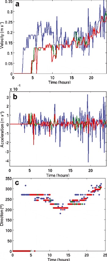
For these test cases, some of the 10 min maximum velocities exceed 0.3 ms– 1, and some of the maximum absolute values of the velocity change rate exceed 0.3 mm s– 2. The ice-drift velocity values are typical: generally 0–1 m s– 1, and in rare cases up to 3 ms– 1 (the ‘ice river’ phenomenon; Reference LeppärantaLeppäranta, 2005). The directions shown in Figures 7 and 8 are rotated by 50° clockwise, i.e. to obtain the actual (compass) directions 50° must be added to the values in the figures. This rotation has been performed to obtain better image coverage of the ship track leading to Kokkola harbor.
The 10 min acceleration is shown in Figures 7b and 8b. Even during the uniform motion (25 February 2011 Tankar case) the 10 min accelerations can be 0.10–0.15 mm s − 2, presumably indicating smaller-scale compression and decompression events within the moving ice field. We also computed estimates of the divergence, based on the motion of the detected objects. Because the object grid is spatially not very dense, divergence values are computed from interpolated motion fields for the object locations. An example of the estimated divergence for two 25 February 2011 case objects is shown in Figure 9. The divergence time series closely follows the acceleration time series in Figure 7b. At the beginning of the ice motion the divergence of the object closer to the opening is higher (green line) than that of the object within the moving ice field (blue line), but later, during the relatively uniform motion, this difference has disappeared. This kind of dynamic ice information is important for fine-scale ice models. It enables the fine-scale dynamic phenomena within sea ice to be modeled better, and the model parameters to be adjusted to the prevailing ice conditions.
Estimated divergence computed for two of the 25 February 2011 examples. The green line corresponds to an object closer to the opening, and the object corresponding to the blue line was located in the middle of the moving ice zone. The divergence estimates are based on the motion of the detected objects and interpolation.
We also studied the change in quality as a function of the tracking time. Typically the quality drops significantly as the ice starts to move, and has lower values for the moving ice objects. The variation between image pairs is typically higher for moving ice. There is also a decreasing trend in quality as the ice moves further from the origin (radar location). Figure 10 shows the quality for the three moving objects in the 2012 case dataset. The decreasing trends, taking into account only the quality values after the objects have started moving (from a tracking time of 5 hours), using a linear least-squares fit, were –0.0069 h − 1, –0.0050 h − 1 and –0.0021 h − 1 for the three tracked ice objects. This reflects the fact that, as the objects move away from the origin, tracking becomes more difficult and finally impossible, i.e. the objects are then lost by the algorithm.
Quality as a function of time for the 2012 Tankar test dataset. In the beginning the objects do not move, and the quality suddenly drops as motion begins. As the objects move away from the origin, a decreasing trend can be seen.
Conclusions and Future Prospects
We have developed an algorithm for selecting and tracking traceable sea-ice objects. Manual selection of the initial objects is also possible. We have demonstrated that the algorithm works well for our two test cases. The object trajectories given by the algorithm can be used instead of ice-drifter buoys to indicate short-time radar-scale ice motion.
Ships, shown as bright dots in radar, are also found and tracked by the algorithm. We are only interested in locating and tracking ice features, not ships. Assuming they are surrounded by open water, the ships can efficiently be removed by removing bright dot-like features. We do not do this here, because ships are typically lost by the algorithm anyway, since it can only find object motion to an upper limit defined by the low resolution and the window size. For example, if the temporal resolution is 10 min, the low spatial resolution is 132 m (4 × 33 m) and the window size is 16 pixels, then motion of 1056 m or less in 10 min, corresponding to 176 cm s − 1 or 6.4 km h − 1, can be detected by the algorithm, and objects with a higher speed are lost. Using such a simple ship-filtering algorithm may also remove small ice segments with high radar backscattering, so some traceable objects may be lost. A more advanced ship filtering could, for example, additionally utilize the ship’s AIS (Automatic Identification System) data to obtain the ship locations, and then perform ship filtering only near the ship locations given by AIS.
The method could probably also be applied to SAR data, though it has not been tested with SAR data yet. The specific problem with SAR data is the coarser temporal resolution, currently 1–3 days over the Baltic Sea. This situation will be improved by the existing and future SAR constellations (COSMO-SkyMed, RADARSAT, Sentinel-1).
The algorithm can be made faster by excluding land points from the computation. Currently we have not applied land masking, and the static land points are included in the computation.
We have not applied any other filtering to the radar data, except the temporal median filtering. To improve the tracking, we could use some kind of noise suppression filtering (e.g. the anisotropic mean filter (Reference Karvonen, Imperatore and RiccioKarvonen, 2010)). Another useful filtering approach would be to apply filtering removing small details. This can be implemented based on image segmentation and then merging the segments with a size lower then a given threshold (e.g. 50 pixels) with the neighboring larger segments, i.e. removing the small segments. After this segment merging, the new filtered image can be produced by computing the segment means for the filtered segmentation. This filtering removes, for example, the small bright dot-like objects, which in many cases are ships or ship lead marks. A disadvantage of the method is that it also removes small ice features, which consist of segments lower than the threshold. However, edge shape details of large segments are not affected by the algorithm. An example of such filtering for one radar image is shown in Figure 11. By using filtered images we could raise the quality threshold T q, because the quality is less reduced by noise.
A detailed example of filtering a radar image. The small details (segments) are removed by this filtering. The size of the details to be removed can be adjusted by a size threshold.

An advantage of this kind of filtering is that the objects in the filtered image represent larger bodies than in the case without filtering, and their change (deformation) rate and motion are typically slower than for very small objects. It is also less likely to create confusion between similar objects in the algorithm, because larger objects typically have a more complex shape than small ones. This filtering not only reduces the number of possible traceable objects, but also reduces the possibility of similarization errors since fewer very small objects are present.
Another possibly applicable filtering technique is to utilize the temporal motion history. At each temporal step, the motion of an object at the previous time-steps can be compared to the current motion candidates, and candidates that deviate too much from the previous motion values can be rejected, leaving only the feasible candidates for the final selection by the maximum phase correlation. This can physically be reasoned by preservation of the motion.
The thresholding of the quality index Q we have used here as a stopping condition for single-object tracking might be improved by adding thresholding of the local image contrast. We would then stop the tracking after either Q becomes lower than T q or the local image contrast measure falls below a contrast threshold. Examples of simple measures of the local image contrast are the local image pixel value standard deviation and the local image pixel value range within an image window.
The statistics of the exact rotation angles could also be included in the algorithm. After locating the drift, the two windows can be sampled in polar coordinates, and the rotation angle can be defined based on the angular shift, corresponding to the maximum correlation in the polar coordinate system.
The resolution of the current system is restricted to one pixel. However, sub-pixel resolution drift can be estimated by interpolating either the correlation or the image windows to be correlated (oversampling). The one-pixel accuracy is typically enough for 10 min time interval tracking, but if we want to perform the tracking at a higher temporal resolution (e.g. 1–2 min), interpolation is required to obtain reliable tracking results. When the ice is moving, a maximal time-series length, for which we can track some features from the beginning to the end of the time series, is typically 24 hours or less, depending on the initial object locations and the magnitude of the drift. We have presented one case of 24 hour tracking, and the tracked objects have already moved close to the range where they are already lost by the algorithm.
We have not performed numerical validation of the algorithm, because we do not have any fine-scale ice-drift reference data within the area covered by the radars. However, we have visually analyzed the image sequences (animations consisting of the image sequences), and noticed that the algorithm tracks the objects reliably, except for the far-range areas, where some errors can occur. Because the quality value reduces towards the far range, this behavior can be corrected using a slightly higher value for the threshold T q. This naturally also leads to earlier loss of the objects.
In future ice seasons, FMI will install image-capturing devices at several coastal stations for operational sea-ice monitoring. We have also performed preliminary experiments with the image-capturing device installed on a ship (R/V Aranda). The ice conditions can also be monitored using an on-board radar, when the ship speed is low enough for the same ice fields to be visible in two adjacent radar images, and the radar images have a long enough temporal difference for radar resolution ice motion to occur. This naturally requires ship motion compensation, which can be done based on the ship-positioning system based on GPS. With efficient and reliable algorithms, coastal radar data can be comprehensively utilized in direct radar-scale ice motion estimation, in fine-scale ice model development and at the final phase of data assimilation into numerical ice models.
Acknowledgement
This work has partly been partially funded by the EC FP-7 SAFEWIN project (reference 233884).


