

1. Introduction
Uncertainty is a major driver in the slow recovery of real economic activity during and after recessions [for surveys, see Bloom (Reference Bloom2014) or Castelnuovo (Reference Castelnuovo2019)]. Most of the existing literature has focused on documenting the aggregate (national) impact of uncertainty on real economic activity [see, e.g. Angelini et al. (Reference Angelini, Bacchiocchi, Caggiano and Fanelli2018); Baker et al. (Reference Baker, Bloom and Davis2016); Bachmann et al. (Reference Bachmann, Elstner and Sims2013); Bloom (Reference Bloom2009); Caggiano et al. (Reference Caggiano, Castelnuovo and Groshenny2014); Carriero et al. (Reference Carriero, Clark and Marcellino2018b); Fernández-Villaverde et al. (Reference Fernández-Villaverde, Guerrón-Quintana, Kuester and Rubio-Ramírez2015); Jurado et al. (Reference Jurado, Ludvigson and Ng2015a); Leduc and Liu (Reference Leduc and Liu2016); Ludvigson et al. (Reference Ludvigson, Ma and Ng2020); Mumtaz and Surico (Reference Mumtaz and Surico2018); Rossi and Sekhposyan (Reference Rossi and Sekhposyan2015) or Scotti (Reference Scotti2016)]. However, the focus on aggregated measures of uncertainty can conceal considerable heterogeneity across areas due to differences, for example, in the composition of production, employment, demographics, and regulations in the financial and public sector. Such differences suggest that greater insights about the role of uncertainty on economic activity can be gained through measuring uncertainty, and identifying its impacts on economic activity, at a more disaggregated area level. Using a model that accommodates potential interactions and spillovers at the disaggregated level, therefore, has the potential to provide new insights into the extent of mitigation or amplification in the transmission of uncertainty across the whole economy.
In this paper, we contribute to the uncertainty literature in a number of ways. First, we propose a novel measure of uncertainty for each of the 51 US states using Google Trends search data (GTU). Along with Bontempi et al. (Reference Bontempi, Golinelli and Squadrani2019) and Castelnuovo and Tran (Reference Castelnuovo and Tran2017), this paper is one of the first to use internet search data to construct an uncertainty index.Footnote 1 The credibility of such an approach to measure uncertainty is illustrated in Castelnuovo and Tran (Reference Castelnuovo and Tran2017) who highlight substantial correlations of the GTU index for the USA as a whole with a variety of different proxies for uncertainty proposed in the literature.Footnote 2 We build on these previous studies by considering the construction and evaluation of disaggregated (state-level) uncertainty indices. We propose that a reliable proxy of uncertainty can be built upon state-specific Google search data on the premise that when economic agents are uncertain about the future, they tend to look for information on the internet. In particular, we focus on uncertainty-related keywords mentioned in the “Beige Books” as published by the Federal Reserve.
The Beige Books gather information on current economic conditions based on interviews with key business contacts, economists, and market experts. Given that the chosen uncertainty-related keywords are those related to influencing business conditions—and that economic agents are more likely to search when there is a higher likelihood of negative economic events—the GTU is most likely to capture the downside risk relevant to the business environment. However, there is also the potential of the index to capture upside risk in the case where firms are looking to make favorable investment decisions in conditions of long-term uncertainty [see Bar-Ilan and Strange (Reference Bar-Ilan and Strange1996) for instance]. Importantly, we find that the GTU index we construct is consistent with other existing uncertainty indices at both the aggregate level as illustrated in Castelnuovo and Tran (Reference Castelnuovo and Tran2017) and with the model-based state-level uncertainty measure in Mumtaz (Reference Mumtaz2018). Therefore, we contend that the use of state-specific Google search data provides real-time, easily accessible and timely information by which to construct measures of uncertainty at the state level for the US economy.
Second, we believe that this is the first paper to explicitly accommodate the dynamic interactions between uncertainty and economic activity across states and across time through a comprehensive and integrated framework. We apply a Global Vector Autoregressive modeling framework [GVAR; elaborated in Garratt et al. (Reference Garratt, Robertson and Wright2006), Dees et al. (Reference Dees, Mauro, Pesaran and Smith2007) and Chudik and Pesaran (Reference Chudik and Pesaran2016)], which jointly models monthly uncertainty and the unemployment rate for the 51 states while allowing for feedback between these variables. The comprehensive specification of this disaggregate model means that we are then able to identify the relative importance of national versus state-specific factors in the propagation of uncertainty shocks on unemployment dynamics at the state level, and their respective associations with a number of state-specific demographic and economic characteristics. Accordingly, existing state-level studies such as Mumtaz et al. (Reference Mumtaz, Sunder-Plassmann and Theophilopoulou2018), Mumtaz (Reference Mumtaz2018) and Shoag and Veuger (Reference Shoag and Veuger2016) are complemented by (1) providing a flexible method for characterizing the evolution over time of the respective state-specific uncertainty and economic activity variables and (2) allowing for relatively complicated forms of interactions and spillover effects between these state-specific variables. Notably, Mumtaz et al. (Reference Mumtaz, Sunder-Plassmann and Theophilopoulou2018) do not measure uncertainty at the state-level but focus only on the impact of national uncertainty on US states, while Mumtaz (Reference Mumtaz2018) and Shoag and Veuger (Reference Shoag and Veuger2016) abstract from state-level feedbacks as well as time dynamics in the propagation of state-level uncertainty.Footnote 3
The importance of disaggregation is relevant to consider in any modeling framework given that the basis of how the economy operates generally involves (highly) interconnected disaggregated units. However, the question of whether a more disaggregate model and particularly, our state-level GTU measures add significant information over an aggregate model will need some formal analysis. First, we judge the statistical adequacy of (linear) aggregate and disaggregate specifications based on the prediction of an aggregate series of interest [see Pesaran et al. (Reference Pesaran, Pierse and Kumar1989) (PPK), Pesaran et al. (Reference Pesaran, Pierse and Lee1994) (PPL) and Van Garderen et al. (Reference Van Garderen, Lee and Pesaran2000) (GLP), for instance]. Second, we investigate the usefulness of the disaggregate model and our state-level GTU uncertainty measures relative to other candidate models through conducting an out-of-sample forecasting exercise. Both analyses provide strong evidence to support the usefulness of disaggregated data in our US state context. The use of a (misspecified) aggregate model therefore would lead us to overlook relevant feedbacks and interactions in the analysis on the impact of uncertainty on the economy.
Moreover, we find that the impact of aggregate uncertainty shocks on unemployment in the disaggregate model, generated as a weighted average of state-level uncertainty shock, is lower compared to the aggregate model, and the dissemination of the uncertainty shocks take almost twice as long relative to the aggregate model. This suggests that the process of aggregation which averages over the heterogeneity in the dynamics concerning the propagation of uncertainty across states, in this context, omits essential dynamics that are significant in driving economic activity at the aggregate level. Although the peak effect is different from a statistical perspective, we still find an important effect of uncertainty shocks in both the models.
In addition, we find that the responses of unemployment in US states to an aggregate uncertainty shock are heterogeneous. The paper provides a narrative to this heterogeneity using various variables capturing state-specific characteristics such as industry composition, fiscal constraints, labor market, and financial frictions in a post-regression analysis. We find that the unemployment rates in states with a larger concentration of the manufacturing industries are affected more by uncertainty shocks, while a larger share of the mining industry mitigates the impact of uncertainty.Footnote 4
In terms of evaluating the relative importance of national factors in propagating the effects of uncertainty shocks on state-level economic activity relative to state-specific factors [see Garratt et al. (Reference Garratt, Lee and Shields2018)], on average, we find the national factors to be less important, although there is significant heterogeneity across states. In general, and as expected, the presence of national factors serves to amplify the effects of uncertainty shocks on state-level unemployment. We then investigate the explanatory power of state-specific characteristics in the heterogeneous importance of the national factors. The results show the relative importance of national influences is greater in states where the real estate sector is greater. It is possible that the larger importance of the national factors in these states reflect the increasing contagion between the financial market and the real estate market during the GFC.Footnote 5 In contrast, we find states with a more active fiscal policy experience a smaller influence of national factors in the impact and propagation of uncertainty shocks. The finding suggests the role of the state government expenditures in offseting the national influences.
The remainder of the paper is organized as follows. Section 2 explains in more detail the construction of the uncertainty index. Section 3 presents the GVAR framework on which this analysis is based. Section 4 outlines the statistical methods for assessing the adequacy of the disaggregate model relative to its aggregate counterpart, investigates the dynamics of the GVAR model, and estimates the impact of uncertainty shocks on economic activity. This section further explores the relative importance of national factors versus state-specific factors in propagating the effect of uncertainty shocks for each state through a decomposition analysis. Section 5 provides a subsequent regression analysis using state-specific characteristics to provide insights into the heterogeneous effects of uncertainty. Section 6 provides some concluding comments.
2. Measuring economic uncertainty
The construction of the uncertainty index is based on the premise that when economic agents, represented by internet users, are uncertain about the future, they tend to look for information on the internet. Under this assumption, the search frequency would be high when the level of uncertainty for a certain topic is high. Google search data is well suited to be the measure of economic uncertainty due to its representative power. According to Comscore (2016), Google has been dominating the online search market in the USA, where its market share has risen 64% in 2016. By exploiting this data-rich environment, the uncertainty index is able to capture the level of uncertainty represented by searchers who are potentially concerned or affected by the state of the economy.
An intuitive example of how to construct a simplified uncertainty index can be found in Appendix 2. It is important to note that, for privacy reasons, Google Trends data does not report the absolute level of queries for a given search term. Instead, Google Trends provides data which gives the frequency of a particular search term relative to the total search volume ranging between 0 and 100. These reported relative search frequencies are constructed as follows. The total search volume for a search term, $R_{{\omega},t,i}$
, where
$R_{{\omega},t,i}$
, where $\omega$
denotes the search term, at time
$\omega$
denotes the search term, at time $t,$
for the location it represents,
$t,$
for the location it represents, $i,$
is divided by the total searches in that geographical region at a point in time,
$i,$
is divided by the total searches in that geographical region at a point in time, $\overline{S}$
:
$\overline{S}$
: $S_{\omega,t,i}=\frac{R_{\omega,t,i}}{\overline{S}_{t,i}}$
.Footnote
6
For exposition purposes, the subscript
$S_{\omega,t,i}=\frac{R_{\omega,t,i}}{\overline{S}_{t,i}}$
.Footnote
6
For exposition purposes, the subscript $i$
is dropped to simplify notation for now.Footnote
7
The resulting numbers are then scaled to a range between 0 and 100, where 100 represents the point where the search frequency is highest,
$i$
is dropped to simplify notation for now.Footnote
7
The resulting numbers are then scaled to a range between 0 and 100, where 100 represents the point where the search frequency is highest, $\text{FI}_{\omega,t}=\frac{100}{M}S_{\omega,t}$
and
$\text{FI}_{\omega,t}=\frac{100}{M}S_{\omega,t}$
and $M=\max \{S_{\omega,1},S_{\omega,2},\ldots,S_{\omega,T}\}$
. Data are excluded if searches are made by very few people. The downside of Google search data, as noted by Choi and Varian (Reference Choi and Varian2009), is that the exact replication of the data is not feasible due to sampling variability, especially for small-volume search terms. This, however, is not an issue in this study, since small-volume search terms play minimal role after the aggregation process which is outlined in what follows.
$M=\max \{S_{\omega,1},S_{\omega,2},\ldots,S_{\omega,T}\}$
. Data are excluded if searches are made by very few people. The downside of Google search data, as noted by Choi and Varian (Reference Choi and Varian2009), is that the exact replication of the data is not feasible due to sampling variability, especially for small-volume search terms. This, however, is not an issue in this study, since small-volume search terms play minimal role after the aggregation process which is outlined in what follows.
The chosen method of aggregating aims to reflect the true search volume relating to each respective search term and, accordingly, a term which is searched more frequently will hold a larger weight in the final aggregated index. As Google only allows the input of a maximum of five different search terms in the Google Trends search engine at any one time, a benchmark term is chosen for the purpose of aggregation since the search frequency provided by Google Trends, $\text{FI}_{\omega,t}$
will alter depending on the choice of the other search terms included in that particular search. This is implemented in the following manner. First, a benchmark term is chosen and entered into the Google Trends search engine together with another search term. The search frequency for the benchmark term in this search is
$\text{FI}_{\omega,t}$
will alter depending on the choice of the other search terms included in that particular search. This is implemented in the following manner. First, a benchmark term is chosen and entered into the Google Trends search engine together with another search term. The search frequency for the benchmark term in this search is $\text{FI}_{\text{benchmark},t}^{1}$
and the output for the other term is
$\text{FI}_{\text{benchmark},t}^{1}$
and the output for the other term is $\text{FI}_{\omega,t}^{1}$
. Second, this process is repeated for the rest of the list of search terms. The frequency of the chosen benchmark term when entered into Google Trends with another search term,
$\text{FI}_{\omega,t}^{1}$
. Second, this process is repeated for the rest of the list of search terms. The frequency of the chosen benchmark term when entered into Google Trends with another search term, $\text{FI}_{\text{benchmark},t}^{2}$
, will not be necessarily the same as the benchmark value in the first step,
$\text{FI}_{\text{benchmark},t}^{2}$
, will not be necessarily the same as the benchmark value in the first step, $\text{FI}_{\text{benchmark},t}^{1}$
as the highest search term in the new combination is automatically set to take a maximum of 100. The search frequency for the remaining search terms in Step 2 is
$\text{FI}_{\text{benchmark},t}^{1}$
as the highest search term in the new combination is automatically set to take a maximum of 100. The search frequency for the remaining search terms in Step 2 is $\text{FI}_{\omega,t}^{2}$
. The true frequency of new search terms (conditional on the search frequency of the benchmark term in Step 1),
$\text{FI}_{\omega,t}^{2}$
. The true frequency of new search terms (conditional on the search frequency of the benchmark term in Step 1), $\text{FI}_{\omega,t}^{1}$
, is calculated by using the adjusting ratio,
$\text{FI}_{\omega,t}^{1}$
, is calculated by using the adjusting ratio, $\text{FI}_{\omega,t}^{1}=\text{FI}_{\omega,t}^{2}\times \frac{\text{FI}_{\text{benchmark},t}^{1}}{\text{FI}_{\text{benchmark},t}^{2}}$
.Footnote
8
$\text{FI}_{\omega,t}^{1}=\text{FI}_{\omega,t}^{2}\times \frac{\text{FI}_{\text{benchmark},t}^{1}}{\text{FI}_{\text{benchmark},t}^{2}}$
.Footnote
8
The Google Trends uncertainty index, $\text{GTU}_{t}$
is the sum of all the scaled search terms where
$\text{GTU}_{t}$
is the sum of all the scaled search terms where $\overline{\omega }$
is the total number of search terms:
$\overline{\omega }$
is the total number of search terms:
 \begin{equation} \text{GTU}_{t}=\sum _{\omega =1}^{\overline{\omega }}\text{FI}_{\omega,t}^{1} \end{equation}
The construction of the index involves identifying which search terms are related to the level of uncertainty in the economy. Our approach is akin to the approach undertaken in Baker et al. (Reference Baker, Bloom and Davis2016) which involved counting the frequency of uncertainty-related words in newspapers. The list of search terms in this paper makes use of the Federal Reserve Bank’s Beige Books. The Beige Book is a summary of economic conditions in the US prepared by the 12 Federal Reserve Districts. Each Federal Reserve Bank gathers anecdotal information on current economic conditions in its District through reports from Bank and Branch directors and interviews with key business contacts, economists, market experts, and other sources. The Beige Book therefore contains valuable information on the factors which contribute to economic agents’ perceptions of uncertainty. When uncertainty is mentioned in a passage, the passage is then examined in more detail to determine the factors which are causing the respective economic agents being interviewed to reveal their uncertainties. These passages are then "human-coded" into a broad set of keywords which are subjectively chosen and which represent such uncertainties. The final set of 85 keywords are presented in Table 1 and form the search terms in Google Trends. Examination of the Beige Book over the past 20 years gives sufficient information on the factors which are accordingly being associated with uncertainty. Consequently, uncertainties are typically related to the banking and finance sector, economic and business conditions, price levels, job market conditions, fiscal and monetary policy, change in regulations, and the housing market.Footnote 9
List of search terms
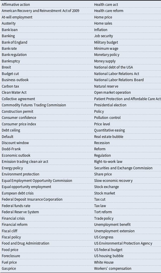
Figure 1 plots the time-varying uncertainty index (GTUit) from 2006M01 to 2018M03, for selected states (i), along with the national uncertainty index, where the national uncertainty index is constructed as the population-weighted average of 51 individual state-level uncertainties in the USA, constructed according to the approach described above. It should be also noted that although the list of search terms is common for all states, the idiosyncratic characteristics of uncertainty measures across different states are driven by differences in perceptions of different sources of uncertainty. While the credibility of the GTU index is illustrated in Castelnuovo and Tran (Reference Castelnuovo and Tran2017) through the strong correlations exhibited with other existing aggregate uncertainty measure, the state-level GTU measures are also found to have considerable correlations with the state-level macroeconomic uncertainty measures constructed in Mumtaz (Reference Mumtaz2018), where the average cross-state correlation is found to be 0.35. In Section 4.2, we conduct a more formal investigation into the usefulness of our state-level GTU measures.
GTU index for selected states in the USA. Notes: The index is transformed to have a mean of 100 and standard deviation of 30. The shaded area represents the Great Recession.

Uncertainty at the state-level and national-level peaks during the Great Recession and returns to more stable levels post-recession. Both state-level uncertainties and the national-level uncertainty show considerable comovements for much of the time.Footnote 10 However, there are period in which there is considerable divergence—in the cases of California and New York, for example. The deviation in New York in June 2011, for instance, is caused by search terms involving austerity, debt ceiling, health care reform, and unemployment benefits. The list of keywords associated with periods of major deviations can be found in Table A3 of the Appendix.
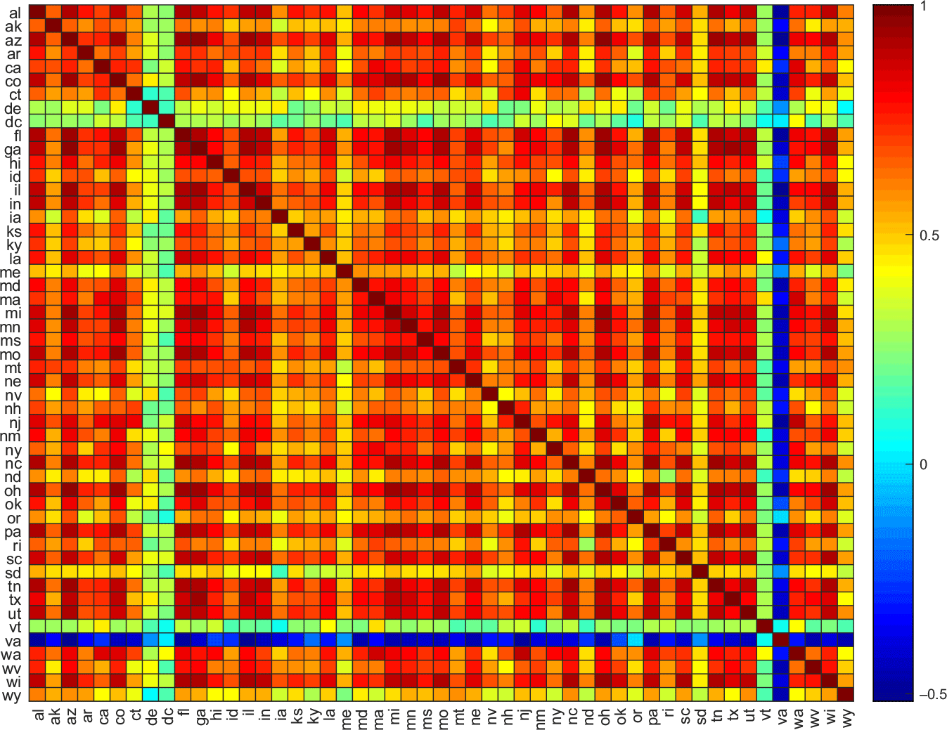
Figure 2 shows the cross-state correlation plot for uncertainty (top panel) and the quarterly change in the unemployment rate (bottom panel). The figure shows a considerable degree of comovement between uncertainty across states and unemployment across states. Conceptually speaking, the idiosyncratic characteristics of uncertainty measures across different states are driven by differences in perceptions of uncertainty. However, it is also the case that the share of internet users can also contribute to such idiosyncratic behavior. The share of internet users are not homogeneous across states, for instance, 65% of the population use the internet in Alabama, while this statistics reaches 80% in California.
Cross-state uncertainty correlation.
3. The modeling framework
The GVAR framework provides an effective way of modeling interactions and feedbacks at a disaggregate state level; such a framework is not only able to interlink the US economy via a common uncertainty channel effect but also takes into account the unobserved interactions. The full technical details of the GVAR model can be found in Section 4 of the Appendix. In essence, the GVAR model is implemented in two steps. In the first step, each individual model explains the state-specific variable, $x_{it}$
, collected in the
$x_{it}$
, collected in the $k_{i}\times 1$
vector; conditional on the cross-sectional averages of all the other state variables, denoted,
$k_{i}\times 1$
vector; conditional on the cross-sectional averages of all the other state variables, denoted, $x_{it}^{\ast }$
, collected in the
$x_{it}^{\ast }$
, collected in the $k_{i}^{\ast }\times 1$
vector. For each state
$k_{i}^{\ast }\times 1$
vector. For each state $i\in 1,\ldots,N$
, a VARX* model is estimated as:
$i\in 1,\ldots,N$
, a VARX* model is estimated as:
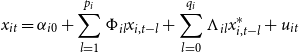 \begin{equation} x_{it}=\alpha _{i0}+\sum _{l=1}^{p_{i}}\Phi _{il}x_{i,t-l}+\sum _{l=0}^{q_{i}}\Lambda _{il}x_{i,t-l}^{\ast }+u_{it} \end{equation}
where $\Phi _{il}$
are
$\Phi _{il}$
are $k_{i}\times k_{i}$
coefficient matrices relating to own respective states,
$k_{i}\times k_{i}$
coefficient matrices relating to own respective states, $\Lambda _{il}$
are
$\Lambda _{il}$
are $k_{i}\times k_{i}^{\ast }$
matrices for "foreign" states, and
$k_{i}\times k_{i}^{\ast }$
matrices for "foreign" states, and $p_{i}$
and
$p_{i}$
and $q_{i}$
are the number of lags for each of these, respectively, and
$q_{i}$
are the number of lags for each of these, respectively, and $\Sigma _{u}$
denotes the variance-covariance matrix of
$\Sigma _{u}$
denotes the variance-covariance matrix of $u_{it}.$
In the second step, these individual state models are then linked and solved simultaneously as one large global VAR model (GVAR). The GVAR model is able to link the individual model together as a global system by using some intuitive weighting matrices that determine the interconnectedness among the individual models such as GDP weights, population weights or even distance weights. In this sense, the aggregate variable in the GVAR model is constructed from individual variables rather than being a true aggregate variable. Population weights are chosen because the correlation between the true US unemployment rate and the aggregated unemployment rate, and the correlation between the true US uncertainty and the aggregated uncertainty are higher relative to when other weighting matrices are used.Footnote 11 The GVAR model is given as:
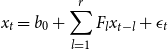 \begin{equation} x_{t}=b_{0}+\sum _{l=1}^r F_{l}x_{t-l}+\epsilon _{t} \end{equation}
where $x_{t}=(x_{0t},x_{1t},\ldots,x_{Nt})^{\prime }$
is the
$x_{t}=(x_{0t},x_{1t},\ldots,x_{Nt})^{\prime }$
is the $k\times 1$
vector that collects all the endogenous variables of the system, and
$k\times 1$
vector that collects all the endogenous variables of the system, and $r=\max \{p_i,q_i\}$
.
$r=\max \{p_i,q_i\}$
.
The GVAR framework therefore allows interactions among different states through three channels: (i) the contemporaneous effect of $x_{it}^{\ast }$
on
$x_{it}^{\ast }$
on $x_{it}$
and its lagged values; (ii) the effect of the common exogenous variable on the state-specific variable; and (iii) the contemporaneous dependence of shocks in state
$x_{it}$
and its lagged values; (ii) the effect of the common exogenous variable on the state-specific variable; and (iii) the contemporaneous dependence of shocks in state $i$
on the shocks in state
$i$
on the shocks in state $j$
.
$j$
.
4. Modeling disaggregated unemployment and uncertainty fluctuations in the USA
4.1 Data
The GVAR framework captures the spillover and feedback effects between uncertainty and unemployment within and across states. The model is estimated using two variables for each state: state-level uncertainty and the state-level unemployment for 51 US states from 2006M01 to 2018M03. Uncertainty for each state is measured according to the method outlined in Section 2 and is in a levels form. Unemployment is measured as the 3-month change in the unemployment rate, measured every month to ensure the stability of the GVAR responses.Footnote 12 The flexibility of this GVAR framework is that it also allows for a relatively parsimonious reduced form representation of the macroeconomy through the accommodation of the effects of aggregate variables—such as interest rates or inflation, for instance, without their necessary explicit inclusion. In essence, to the extent that such aggregate variables are important determinants of state-specific unemployment, their heterogenous effects will be captured through current and lagged values of the starred variables.Footnote 13
Due to the short time span of the Google search data, the maximum $p_{i}$
is 2 and the maximum
$p_{i}$
is 2 and the maximum $q_{i}$
is 1 following Dees et al. (Reference Dees, Mauro, Pesaran and Smith2007).Footnote
14
Based on the Akaike information criterion (AIC), a VARX*(1,1) is fitted to most states. A specification search is also performed on the coefficients and insignificant coefficients for which the absolute value of the
$q_{i}$
is 1 following Dees et al. (Reference Dees, Mauro, Pesaran and Smith2007).Footnote
14
Based on the Akaike information criterion (AIC), a VARX*(1,1) is fitted to most states. A specification search is also performed on the coefficients and insignificant coefficients for which the absolute value of the $t$
-ratio being less than 1 are excluded from the model.Footnote
15
$t$
-ratio being less than 1 are excluded from the model.Footnote
15
4.2 Assessing the Adequacy of the Disaggregate Model
4.2.1 Joint significance
The joint significance of the foreign variables
GVAR models allow for potentially important cross-state interaction information that cannot be explicitly captured in more aggregate models. As described earlier, the presence of the starred or foreign variables allow uncertainty and unemployment to be interconnected across states that are represented by the coefficient matrices $\Lambda$
. To investigate the statistical importance of these variables, however, the joint significance of cross-state interactions is calculated through an F-test of the joint significance of starred uncertainty variables and starred unemployment variables in each of the uncertainty and the unemployment equations for each of the individual state models.
$\Lambda$
. To investigate the statistical importance of these variables, however, the joint significance of cross-state interactions is calculated through an F-test of the joint significance of starred uncertainty variables and starred unemployment variables in each of the uncertainty and the unemployment equations for each of the individual state models.
Table 2 reports the F-test statistics associated with testing of the following null: $H_{0}:\Lambda _{i0}^{\tau }=\Lambda _{i1}^{\tau }=0$
for
$H_{0}:\Lambda _{i0}^{\tau }=\Lambda _{i1}^{\tau }=0$
for $i=1,\ldots,N$
and for
$i=1,\ldots,N$
and for $\tau =1,\ldots,4$
.Footnote
16
The table shows that there is significant statistical evidence showing the importance of starred uncertainty and starred unemployment in each of the state-specific equations. In other words, there is evidence of substantial interaction of economic activity and behavior across disaggregate units and therefore gives support to the use of the GVAR modeling approach as an appropriate framework to capture these complex interactions.
$\tau =1,\ldots,4$
.Footnote
16
The table shows that there is significant statistical evidence showing the importance of starred uncertainty and starred unemployment in each of the state-specific equations. In other words, there is evidence of substantial interaction of economic activity and behavior across disaggregate units and therefore gives support to the use of the GVAR modeling approach as an appropriate framework to capture these complex interactions.
F-test statistics on the joint significance of national uncertainty ( $us^*$
) and national unemployment (
$us^*$
) and national unemployment ( $ur^*$
)
$ur^*$
)
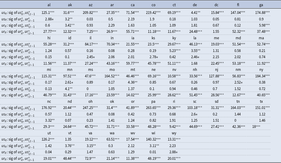
Notes: This shows the F-test statistics of the joint significance of national uncertainty ( $us*$
) and national unemployment (
$us*$
) and national unemployment ( $ur*$
) of the state-level uncertainty and unemployment equations
$ur*$
) of the state-level uncertainty and unemployment equations $^{***}p\lt 0.01$
,
$^{***}p\lt 0.01$
, $^{**}p\lt 0.05$
,
$^{**}p\lt 0.05$
, $^{*}p\lt 0.1$
.
$^{*}p\lt 0.1$
.
The Joint Significance of the State-Specific Uncertainty Variables
Given there are substantial interactions between uncertainty measures across states, we next investigate whether our state-specific uncertainty measures provide meaningful information content in describing the variation in uncertainty above and beyond the information already provided by the aggregate or common factor element. To investigate the statistical importance of the idiosyncratic uncertainty component, therefore, the joint significance is calculated through an F-test of the joint significance of state-specific uncertainty in each of the uncertainty and the unemployment equations for each of the individual state models.
Table 3 reports the F-test statistics associated with testing of the following null: $H_{0}:\Phi _{i1}^{\upsilon }=\Phi _{i2}^{\upsilon }=0$
for
$H_{0}:\Phi _{i1}^{\upsilon }=\Phi _{i2}^{\upsilon }=0$
for $i=1,\ldots,N$
and for
$i=1,\ldots,N$
and for $\upsilon =1,2$
.Footnote
17
The table shows that there is significant statistical evidence showing the importance of idiosyncratic uncertainty component in almost all states. On the whole, despite the substantial interaction of economic activity across states, there is evidence that the idiosyncratic components also provide meaningful contributions in explaining fluctuations in state-level economic activity and uncertainty.
$\upsilon =1,2$
.Footnote
17
The table shows that there is significant statistical evidence showing the importance of idiosyncratic uncertainty component in almost all states. On the whole, despite the substantial interaction of economic activity across states, there is evidence that the idiosyncratic components also provide meaningful contributions in explaining fluctuations in state-level economic activity and uncertainty.
F-test statistics on the joint significance of state-specific uncertainty ( $us$
)
$us$
)
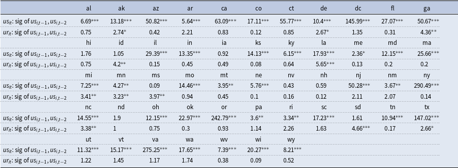
Notes: This shows the F-test statistics of the joint significance of state uncertainty ( $us$
) of the state-level uncertainty and unemployment equations
$us$
) of the state-level uncertainty and unemployment equations $^{***}p\lt 0.01$
,
$^{***}p\lt 0.01$
, $^{**}p\lt 0.05$
,
$^{**}p\lt 0.05$
, $^{*}p\lt 0.1$
.
$^{*}p\lt 0.1$
.
4.2.2 Predictive criteria
This section makes use of a statistical criterion to investigate the usefulness of disaggregate data in understanding the effect of uncertainty at the US state and national level. While a well-specified disaggregated model will generally outperform an aggregate model, if the disaggregate model is misspecified, this may not hold. For instance, a disaggregate model may be misspecified if macroeconomic influences are incorrectly omitted or if measurement errors found in the disaggregate model cancel out in the aggregate. The inclusion of the global variables in the GVAR model means that the first will unlikely to be a problem; however, the second might be potentially relevant due to the sample size of the Google data. The prediction criteria test proposed in PPK assesses the ability of a disaggregate model in predicting an aggregate series of interest, relative to the ability of an aggregate model, under the null that the disaggregate model is true.
In this context, assume that each state, $i,$
is modeled according to the VARX* model specified earlier and that the aggregate model is assumed to be estimated of the following vector form:
$i,$
is modeled according to the VARX* model specified earlier and that the aggregate model is assumed to be estimated of the following vector form:
 \begin{equation} y_{t}=c_{t}+\mathbf{a}y_{t-1}+\mathbf{b}y_{t-2}+\mathbf{e}_{t}. \end{equation}
where $y_{t}=\left (US_{t},UR_{t}\right )$
,
$y_{t}=\left (US_{t},UR_{t}\right )$
, $US_{t}=\sum _{i=1}^{s}w_{i}us_{i,t}$
and
$US_{t}=\sum _{i=1}^{s}w_{i}us_{i,t}$
and $UR_{t}=\sum _{i=1}^{s}w_{i}ur_{i,t}$
.Footnote
18
$UR_{t}=\sum _{i=1}^{s}w_{i}ur_{i,t}$
.Footnote
18
In PPK, the following statistics are used to rank the disaggregate model and the aggregate model:
 \begin{equation} s_{a}^{2}=\frac{\mathbf{e_{t}}^{\prime }\mathbf{e_{t}}}{T-\kappa _{a}}, \end{equation}
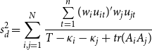 \begin{equation} s_{d}^{2}=\sum _{i,j=1}^{N}\frac{\sum \limits _{t=1}^{n}(w_{i}u_{it})^{\prime }w_{j}u_{jt}}{T-\kappa _{i}-\kappa _{j}+tr(A_{i}A_{j})} \end{equation}
where $T$
is the number of observations,
$T$
is the number of observations, $\kappa _{a}$
is the number of estimated parameters in the aggregate model,
$\kappa _{a}$
is the number of estimated parameters in the aggregate model, $\kappa _{i}$
is the number of unrestricted parameters in each disaggregate model, and
$\kappa _{i}$
is the number of unrestricted parameters in each disaggregate model, and $A_{i}=X_{i}(X_{i}^{\prime }X_{i})^{-1}X_{i}^{\prime }$
, and
$A_{i}=X_{i}(X_{i}^{\prime }X_{i})^{-1}X_{i}^{\prime }$
, and $X_{i}$
is the matrix which consists of the explanatory variables in the
$X_{i}$
is the matrix which consists of the explanatory variables in the $i$
-th equation. These statistics have the property that on average
$i$
-th equation. These statistics have the property that on average $s_{a}^{2}\gt s_{d}^{2}$
if the disaggregate model is true. Lee and Shields (Reference Lee and Shields1998) transform
$s_{a}^{2}\gt s_{d}^{2}$
if the disaggregate model is true. Lee and Shields (Reference Lee and Shields1998) transform $s_{a}^{2}$
and
$s_{a}^{2}$
and $s_{d}^{2}$
to statistics that are comparable to
$s_{d}^{2}$
to statistics that are comparable to $R^{2}$
measures:
$R^{2}$
measures:
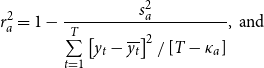 \begin{equation} r_{a}^{2} =1-\frac{s_{a}^{\text{2}}}{\sum \limits _{t=1}^{T}\left [ y_{t}-\overline{y_{t}}\right ] ^{2}/\left [ T-\kappa _{a}\right ]},\text{ and} \end{equation}
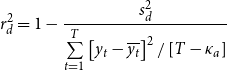 \begin{equation} r_{d}^{2} =1-\frac{s_{d}^{\text{2}}}{\sum \limits _{t=1}^{T}\left [ y_{t}-\overline{y_{t}}\right ] ^{2}/\left [ T-\kappa _{a}\right ]} \end{equation}
where $\overline{y_{t}}$
represents the mean of the aggregate uncertainty and unemployment series, and
$\overline{y_{t}}$
represents the mean of the aggregate uncertainty and unemployment series, and $r_{a}$
and
$r_{a}$
and $r_{d}$
denote the transformed prediction criteria for the aggregate and disaggregate model, respectively. In this case, on average,
$r_{d}$
denote the transformed prediction criteria for the aggregate and disaggregate model, respectively. In this case, on average, $r_{a}^{2}$
will be smaller than
$r_{a}^{2}$
will be smaller than $r_{d}^{2}$
if the disaggregate model is true. Asymptotically, if the disaggregate model is true, the criterion discussed above will rank the models correctly, on average, but this may not hold in a finite sample. To assess this, following GLP, a simulation experiment can be carried out by simulating the distribution of the test statistic,
$r_{d}^{2}$
if the disaggregate model is true. Asymptotically, if the disaggregate model is true, the criterion discussed above will rank the models correctly, on average, but this may not hold in a finite sample. To assess this, following GLP, a simulation experiment can be carried out by simulating the distribution of the test statistic, $D_{ad}=r_{d}^{2}-r_{a}^{2},$
defining the difference between the choice criteria. Accordingly, if the disaggregate model is correctly specified,
$D_{ad}=r_{d}^{2}-r_{a}^{2},$
defining the difference between the choice criteria. Accordingly, if the disaggregate model is correctly specified, $D_{ad}\gt 0.$
However, although this will hold asymptotically, this statistic may be smaller than 0 in any particular sample simply because of sample variation.Footnote
19
Given this, GLP suggest calculating a value
$D_{ad}\gt 0.$
However, although this will hold asymptotically, this statistic may be smaller than 0 in any particular sample simply because of sample variation.Footnote
19
Given this, GLP suggest calculating a value $d_{ad}^{\ast }(\alpha )$
obtained from the distribution of
$d_{ad}^{\ast }(\alpha )$
obtained from the distribution of $D_{ad}$
such that the probability of selecting the disaggregate model when it is true is
$D_{ad}$
such that the probability of selecting the disaggregate model when it is true is $(1-\alpha )$
. We do so by first simulating the data 5000 times, assuming that the structure of the disaggregate model is the true data-generating process, and sampling with replacement. At each run, the test statistic is recalculated to obtain the distribution for
$(1-\alpha )$
. We do so by first simulating the data 5000 times, assuming that the structure of the disaggregate model is the true data-generating process, and sampling with replacement. At each run, the test statistic is recalculated to obtain the distribution for $D_{ad}$
, and the value of
$D_{ad}$
, and the value of $d_{ad}^{\ast }(\alpha )$
is determined from the left tail of this distribution.
$d_{ad}^{\ast }(\alpha )$
is determined from the left tail of this distribution.
We find significant statistical evidence that the disaggregate model outperforms the aggregate model in terms of its ability to predict aggregate uncertainty and aggregate unemployment as shown in Figure 3. Figure 3 reports the predictive difference between the aggregate model and the disaggregate model in predicting uncertainty (top panel) and unemployment (middle panel)—that is $D_{ad}=r_{d}^{2}-r_{a}^{2}$
along
$D_{ad}=r_{d}^{2}-r_{a}^{2}$
along $d_{ad}^{\ast }(\alpha )$
from the simulated distribution (
$d_{ad}^{\ast }(\alpha )$
from the simulated distribution ( $\alpha =0.05$
). The figure clearly shows that the disaggregate model displays a higher ability to predict uncertainty and unemployment compared to the aggregate model, as seen by positive
$\alpha =0.05$
). The figure clearly shows that the disaggregate model displays a higher ability to predict uncertainty and unemployment compared to the aggregate model, as seen by positive $D_{ad}$
values (in red). Further, once random variation is taken into account, there is still significant evidence to support the use of the disaggregate model, as illustrated by the fact the test statistics for predicting uncertainty and unemployment are both larger and on the right of the left tails of the distribution,
$D_{ad}$
values (in red). Further, once random variation is taken into account, there is still significant evidence to support the use of the disaggregate model, as illustrated by the fact the test statistics for predicting uncertainty and unemployment are both larger and on the right of the left tails of the distribution, $d_{ad}^{\ast }(\alpha )$
.
$d_{ad}^{\ast }(\alpha )$
.
Prediction criteria. Notes: This figure plots the observed $D_{ad}$
, which is the difference in the prediction criteria test statistic (red line) and
$D_{ad}$
, which is the difference in the prediction criteria test statistic (red line) and $d^*_{ad}(\alpha )$
, which is the left tail of the simulated distribution of the prediction criteria test statistic (dotted blue line) and assesses the ability of the disaggregate model versus the aggregate model in predicting aggregate uncertainty and aggregate unemployment, respectively. The figure also plots the observed
$d^*_{ad}(\alpha )$
, which is the left tail of the simulated distribution of the prediction criteria test statistic (dotted blue line) and assesses the ability of the disaggregate model versus the aggregate model in predicting aggregate uncertainty and aggregate unemployment, respectively. The figure also plots the observed $D_{dpard}$
, which is the difference in the prediction criteria test statistic (red line) and
$D_{dpard}$
, which is the difference in the prediction criteria test statistic (red line) and $d^*_{dpard}(\alpha )$
, which is the left tail of the simulated distribution of the prediction criteria test statistic (dotted blue line) and assesses the ability of the disaggregate model versus the partial disaggregate model without state-level uncertainty in predicting unemployment.
$d^*_{dpard}(\alpha )$
, which is the left tail of the simulated distribution of the prediction criteria test statistic (dotted blue line) and assesses the ability of the disaggregate model versus the partial disaggregate model without state-level uncertainty in predicting unemployment.
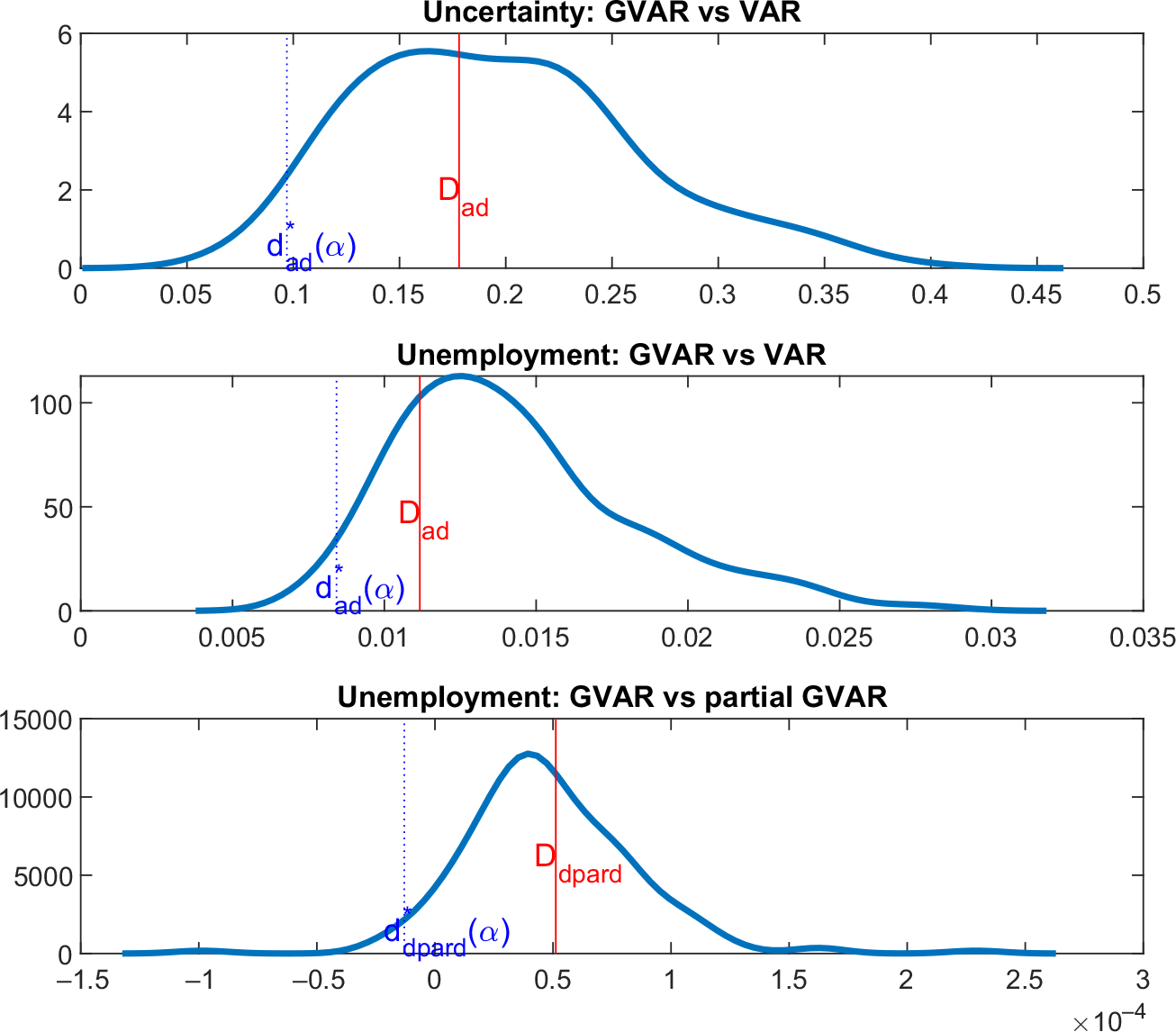
In the second exercise, we specifically investigate the value-added of our state-level measures of uncertainty in the disaggregate model, which again tests for the importance of the explanatory power of state-level measures of uncertainty above and beyond that of the common component. The previous exercise showed that a disaggregate model with state-level uncertainty measures and the state-level unemployment outperforms the aggregate model in terms of predicting aggregate variables. We further investigate whether the same disaggregate model outperforms a partial disaggregate model, which does not feature state-level measures of uncertainty, in terms of predicting the aggregate unemployment variable, under the null that the full disaggregate model is true. We find significant statistical evidence that the full disaggregate model outperforms the partial disaggregate model as shown in the bottom panel of Figure 3. This is reflected in the figure by a positive $D_{dpard}$
value (in red). Further, once random variation is taken into account, there is still significant evidence to support the use of the disaggregate model, as illustrated by the fact the test statistics for predicting unemployment are both larger and on the right of the left tail of the distribution,
$D_{dpard}$
value (in red). Further, once random variation is taken into account, there is still significant evidence to support the use of the disaggregate model, as illustrated by the fact the test statistics for predicting unemployment are both larger and on the right of the left tail of the distribution, $d_{dpard}^{\ast }(\alpha )$
.
$d_{dpard}^{\ast }(\alpha )$
.
4.2.3 Forecast performance
Table 4 presents the out-of-sample forecast performance in terms of both point forecasts, as measured by the Root Mean Squared Errors (RMSEs) and density forecasts, as measured by the Average Log Scores (ALSs) of various models in predicting aggregate unemployment at the 1-month, 3-month, 6-month, and 1-year forecast horizons in purely statistical terms. We perform the out-of-sample evaluation using a rolling window estimation scheme over two sample horizons. In the first exercise, we use half the sample period (from 2006M01 to 2012M01) as the initial sample size and forecast using a rolling window until 2015M02 (which represents 3/4 of the total sample size). In the second, observations up to 2015M02 are used as the initial period to form out-of-sample forecasts for the remaining sample. The GVAR model in equation (3) is used as the benchmark to illustrate the usefulness of our disaggregate framework as well as of our state-level GTU measures. A value less than 1 represents a superior forecasting performance. The table reports the improvement or deterioration in forecast performance of the GVAR model relative to other forecasting models, namely (i) disaggregate model of state-level unemployment using only unemployment variables (DISU); (ii) a partially disaggregated model using state-level measures of unemployment alongside the aggregate GTU measure of uncertainty (GTU); (iii)–(vi) as the model in (ii) but respectively using the EPU [Baker et al. (Reference Baker, Bloom and Davis2016)], the VIX, a measure of macroeconomic uncertainty (JLN) [Jurado et al. (Reference Jurado, Ludvigson and Ng2015a)] and a measure of financial uncertainty (LMN) [Ludvigson et al. (Reference Ludvigson, Ma and Ng2020)], in place of the GTU as the aggregate measures of uncertainty. The statistical significance of the improvement is tested using the Giacomini and White (Reference Giacomini and White2006) test of equal forecast performance.
Evaluation of out-of-sample point and density forecasts

Notes: The upper (lower) panel reports the out-of-sample RMSE (Average Log Scores—ALS) ratio of the GVAR model relative to the RMSE (ALS) of other models. A ratio $\lt$
1 indicates that the GVAR model outperforms other models. A "
$\lt$
1 indicates that the GVAR model outperforms other models. A " $^*$
" denotes that the RMSE (ALS) ratio for the GVAR model statistically outperforms the other models at the 10% level of significance through applying the Giacomini and White (Reference Giacomini and White2006) test of equal forecast performance. We perform the out-of-sample evaluation using a rolling window estimation scheme.
$^*$
" denotes that the RMSE (ALS) ratio for the GVAR model statistically outperforms the other models at the 10% level of significance through applying the Giacomini and White (Reference Giacomini and White2006) test of equal forecast performance. We perform the out-of-sample evaluation using a rolling window estimation scheme. $T$
is the total sample size and is out of 1 (100%) and
$T$
is the total sample size and is out of 1 (100%) and $t0$
is the training sample size.
$t0$
is the training sample size.
The top half of Table 4 presents the forecasting performance using the RMSE criterion and shows that there is not much evidence from the point forecasts. The GVAR outperforms the diasaggrate model using unemployment only (DISU) and the partially disaggregated models in the case of the measure of macroeconomic uncertainty (JLN). Only in the latter case, however, the performance is statistically significant. The bottom half of the table presents the forecasting results using the density-based ALS. The results show that the extra complexity of GVAR stemming from our state-level uncertainty measures has an important impact on forecast performance. The GVAR benchmark outperforms in five of the six models, and the forecast performance is statistically significant. There is therefore strong evidence to support the usefulness of the disaggregate model in a broad sense and, in particular, the usefulness of our measures of state-level uncertainty over and beyond the information provided by other uncertainty measures that are only available at the aggregate level.
4.3 Dynamic Impulse Response Analysis
The identification of exogenous variations of the uncertainty shock is achieved via the widely adopted time-ordering assumption. A recent paper by Carriero et al. (Reference Carriero, Clark and Marcellino2018a) shows that macroeconomic uncertainty can be considered as exogenous when assessing its effects on the US economy. Nonetheless, our general conclusions are robust to this time-ordering assumption (see Section 8 of the Appendix for further details). In addition, it is noticed that the construction of our uncertainty index includes terms such as "unemployment benefit" or "unemployment extension" which may raise endogeneity concerns. We find that it is not the case since the average correlation between the original uncertainty and the index without these unemployment-related keywords gives the value close to 0.99. In addition, following Garín et al. (Reference Garín, Lester and Sims2019), we also find that the GTU index is uncorrelated with other shocks such as total factor productivity, oil price, fiscal, or monetary policy shocks. The ordering implies that uncertainty does not respond to the unemployment shock in the impact period while allowing unemployment to respond to the uncertainty shock (while still allowing uncertainty shocks between states to be correlated). This also assigns the maximum possible effect to the uncertainty shocks and provides an upper bound on the measure of the effect of uncertainty.
Consider the GVAR(2) model in equation (3), the moving average representation is given by:
 \begin{equation} x_{t}=\epsilon _{t}+A_{1}\epsilon _{t-1}+A_{2}\epsilon _{t-2}+\ldots \end{equation}
and $A_{s}$
can be defined recursively as:
$A_{s}$
can be defined recursively as:
 \begin{equation} A_{s}=F_{1}A_{s-1}+F_{2}A_{s-2},\ \ s=1,2,\ldots \end{equation}
with $A_{0}$ $=I$
,
$=I$
, $A_{s}=0$
for
$A_{s}=0$
for $s\lt 0$
.
$s\lt 0$
.
The time-ordering assumption of the shocks allows us to separate the effects of the uncertainty shocks, denoted as $\delta _{t}=(\epsilon _{1t},\epsilon _{3t},\ldots,\epsilon _{101t})$
, from the total shocks to the GVAR by regressing
$\delta _{t}=(\epsilon _{1t},\epsilon _{3t},\ldots,\epsilon _{101t})$
, from the total shocks to the GVAR by regressing $\epsilon _{t}$
on
$\epsilon _{t}$
on $\delta _{t}$
and writing
$\delta _{t}$
and writing $\epsilon _{t}=\bar{D}\delta _{t}+\tilde{\epsilon _{t}}$
. In this case, equation (9) can be rewritten in terms of "orthogonal" uncertainty shocks and other unemployment-related shocks:
$\epsilon _{t}=\bar{D}\delta _{t}+\tilde{\epsilon _{t}}$
. In this case, equation (9) can be rewritten in terms of "orthogonal" uncertainty shocks and other unemployment-related shocks:
 \begin{equation} x_{t}=\left [ \bar{D}\delta _{t}+\tilde{\epsilon _{t}}\right ] +A_{1}[\bar{D}\delta _{t-1}+\tilde{\epsilon }_{t-1}]+A_{2}[\bar{D}\delta _{t-2}+\tilde{\epsilon }_{t-2}]+\ldots \end{equation}
The impulse response function for the GVAR model can then be written as:
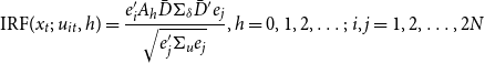 \begin{equation} \text{IRF}(x_{t};\;u_{it},h)=\frac{e_{i}^{\prime }A{_{h}}\bar{D}\Sigma _{\delta }\bar{D}^{\prime }e_{j}}{\sqrt{e_{j}^{\prime }\Sigma _{u}e_{j}}},h=0,1,2,\ldots ;\; i,j=1,2,\ldots,2N \end{equation}
where $\Sigma _{\delta }$
denotes the variance–covariance matrix of the uncertainty shocks,
$\Sigma _{\delta }$
denotes the variance–covariance matrix of the uncertainty shocks, $\delta _{t},$ $e_{i}$
, and
$e_{i}$
, and $e_{j}$
are
$e_{j}$
are $2N\times 1$
selection vectors with unity in their
$2N\times 1$
selection vectors with unity in their $i$
-th
$i$
-th $,$
$,$ $j$
-th elements, respectively, and zeros elsewhere, and
$j$
-th elements, respectively, and zeros elsewhere, and $h$
is the horizon of the impulse. For an aggregate shock,
$h$
is the horizon of the impulse. For an aggregate shock, $e_{i}$
is a vector of aggregate weights in the elements of
$e_{i}$
is a vector of aggregate weights in the elements of $j=2,4,6,\ldots,2N,$
in the case of a national unemployment shock for instance, where the weights sum to 1 and where population weights are chosen to be consistent with the construction of the starred variables in the GVAR model. Given the identification assumption, the effect of a one-standard-deviation population-weighted aggregate uncertainty shock on the (weighted aggregate) unemployment variable in the GVAR model can be seen in Figure 4. For illustrative purposes, this figure also reports the traditional orthogonalized impulse response function for the bivariate VAR aggregate model showing the impact of an orthogonal uncertainty shock (defined through a Cholesky decomposition) on the unemployment variable.
$j=2,4,6,\ldots,2N,$
in the case of a national unemployment shock for instance, where the weights sum to 1 and where population weights are chosen to be consistent with the construction of the starred variables in the GVAR model. Given the identification assumption, the effect of a one-standard-deviation population-weighted aggregate uncertainty shock on the (weighted aggregate) unemployment variable in the GVAR model can be seen in Figure 4. For illustrative purposes, this figure also reports the traditional orthogonalized impulse response function for the bivariate VAR aggregate model showing the impact of an orthogonal uncertainty shock (defined through a Cholesky decomposition) on the unemployment variable.
Aggregate uncertainty shocks on aggregate unemployment. Notes: This figure compares the IRFs of a one-standard-deviation aggregate uncertainty shock in the GVAR model to the VAR model. The GVAR IRFs are the weighted response of each state unemployment to an aggregate uncertainty shock in the GVAR model, where the aggregate shock is defined in equation (12) through using population weights. The VAR IRFs are constructed via the Cholesky decomposition where uncertainty is placed first. Unemployment is defined as the quarterly change in unemployment rate. The confidence interval is the bootstrapped IRFs at $\pm 1$
s.d.
$\pm 1$
s.d.

Although the effects of the respective uncertainty shocks on unemployment in both the aggregate model and the disaggregate model are similar, we find that the impact of an aggregate uncertainty shock in the disaggregate model is significantly smaller than in the aggregate model when we look at the peak response of unemployment. We find that the quarterly change in unemployment rate in the disaggregate model goes up by 0.015% point at peak, compared to 0.045% point in the aggregate model. Since unemployment is modeled as the quarterly change in the unemployment rate, we could recover the response of the actual unemployment rate to provide intuitive interpretations on the effect of uncertainty shocks. We find that the peak effect of uncertainty shock in the disaggregate GVAR model causes the unemployment rate to go up by 0.1% points. On the other hand, the unemployment rate goes up by 0.28% points in the aggregate model at peak. These findings are within the bounds of the measures documented in the literature.Footnote 20
On the whole, even after assigning uncertainty to have maximum effects due to the time-ordering assumption, our results are shown to be at the more conservative end of the impact of uncertainty on economic activity. In terms of the dynamics, both impulse responses tend to start dying away after 2 years, although, the GVAR model, despite providing a smaller peak response effect, shows a far more prolonged process of dissemination of the initial shock taking approximately double the time of the impulse response from the VAR model which rapidly disseminates after approximately 2 years.
In sum, both modeling frameworks point to the significant effect of uncertainty on unemployment. The use of an aggregate model, however, shown to be misspecified in the previous section, accordingly averages over relevant feedbacks and interactions through the process of aggregation in the analysis of the impact of uncertainty on the economy and therefore overestimates the effects of uncertainty shocks relative to the disaggregate model. The aggregate model also underestimates the time it takes for the uncertainty shock to work its way through the system. As a result, the disaggregate model shows the effect of an uncertainty shock on unemployment to be statistically and significantly smaller than that according to the aggregate model and with a relatively far more prolonged dynamic response.
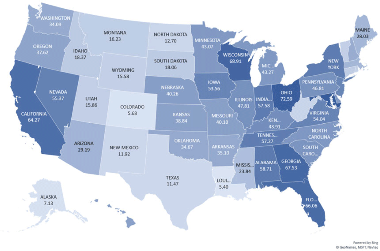
We close this section by observing whether there are any spatial patterns apparent in the heterogeneous responses of state-level unemployment to an aggregate uncertainty shock. In a heatmap of the USA, Figure 5 presents the median estimate of the peak response of state-level unemployment to a one-standard-deviation aggregate uncertainty shock. We find that unemployment increases in all states in response to an increase in US-wide uncertainty. The findings are also consistent to those documented in Mumtaz et al. (Reference Mumtaz, Sunder-Plassmann and Theophilopoulou2018) who find that real income declines in all states in response to an increase in US-wide uncertainty (even without accommodating for state-level uncertainty). The figure also shows that the magnitude of the increase in unemployment is largest in the coastal states. On the other hand, unemployment in more central states in the USA seems to be less affected. These heterogeneous responses in the response of unemployment to uncertainty shocks could potentially be driven by cross-state variations in financial and fiscal conditions, the industry mix, and the labor market. We investigate this in more detail in Section 5.
US heatmap—peak response of state-level unemployment to an aggregate uncertainty shock. Notes: This figure presents the median estimate of the peak response of state-level unemployment to a one-standard-deviation aggregate uncertainty shock.

4.4 Decomposition Analysis: State versus National Influences
In this section, we explore, for each state, the relative importance of national influences relative to state-specific influences of a national uncertainty shock on state-level economic activity. This section follows Garratt et al. (Reference Garratt, Lee and Shields2018) and characterizes the dynamic effects of specified shocks by using the variance-based persistence profile (PP) measure proposed by Lee and Pesaran (Reference Lee and Pesaran1993). The PP is used to measure the long-run response of the level series to shocks and trace out the accumulated response over time to characterize the system dynamics.
At time horizon $h$
, the PPs are defined by the
$h$
, the PPs are defined by the $2N\times 2N$
matrix
$2N\times 2N$
matrix $P(h)$
and as
$P(h)$
and as $h\rightarrow \infty$
, converges to the following persistence matrix, in which the
$h\rightarrow \infty$
, converges to the following persistence matrix, in which the $(i,j)$
-th element is given by:
$(i,j)$
-th element is given by:
 \begin{equation} p_{ij}=\frac{e_{i}^{\prime }A(1)\Sigma _{\epsilon }A(1)^{\prime }e_{j}}{\sqrt{(e_{i}^{\prime }A(0)\Sigma _{\epsilon }A(0)^{\prime }e_{i})(e_{j}^{\prime }A(0)\Sigma _{\epsilon }A(0)^{\prime }e_{j}})}, \qquad \qquad i,j=1,\ldots,2N, \end{equation}
where $p_{ij}$
measures the infinite horizon effect of system-wide shocks to variables in the system. For instance, the permanent impact on unemployment in each state of a system-wide shock which causes the unemployment variable in each state to rise by 1 standard error on impact can be captured by considering the measures
$p_{ij}$
measures the infinite horizon effect of system-wide shocks to variables in the system. For instance, the permanent impact on unemployment in each state of a system-wide shock which causes the unemployment variable in each state to rise by 1 standard error on impact can be captured by considering the measures $p_{ii},$
where
$p_{ii},$
where $i=2,4,6,\ldots 2N$
and where
$i=2,4,6,\ldots 2N$
and where $i=j$
.
$i=j$
.
For the sake of brevity, the full technical details of the decomposition can be found in Section 11 of the Appendix. In this analysis, two decompositions of the persistence measure $p_{ii}$
are of interest. The first concerns the part due to orthogonalized uncertainty shocks on state unemployment dynamics relative to other unidentified unemployment-related shocks (
$p_{ii}$
are of interest. The first concerns the part due to orthogonalized uncertainty shocks on state unemployment dynamics relative to other unidentified unemployment-related shocks ( $p^U_{ii}$
), and this decomposition makes use of the orthogonalization of uncertainty shocks as described in the previous section. The second concerns the decomposition of the dynamic propagation of these uncertainty shocks (
$p^U_{ii}$
), and this decomposition makes use of the orthogonalization of uncertainty shocks as described in the previous section. The second concerns the decomposition of the dynamic propagation of these uncertainty shocks ( $p^U_{ii}$
) into the components due to national dynamics (
$p^U_{ii}$
) into the components due to national dynamics ( $p^{NU}_{ii}$
) relative to state-specific dynamics (
$p^{NU}_{ii}$
) relative to state-specific dynamics ( $p^{SU}_{ii}$
), focusing on the infinite horizon effect on state-specific unemployment.
$p^{SU}_{ii}$
), focusing on the infinite horizon effect on state-specific unemployment.
Figure 6 reports the ratio: $\frac{p_{ii}^{NU}}{p_{ii}^{U}}$
in a heatmap of the USA, which gives the relative importance of national dynamics versus both state and national dynamics, as modeled in equation (3), in terms of respective measures of the persistent effect of the above-defined uncertainty shocks on state-specific unemployment. The persistence measures are scaled by a standard error state-specific unemployment shock on impact. A simple correlation between the statistics for each state represented in Figure 5 and those in Figure 6 gives a value of 0.4 showing that national influences play a clear role in propagating the effects of uncertainty. On average, the uncertainty shocks transmitted through the channels associated with national elements account for 37% of the total variation in state-specific unemployment and the remaining 63% is attributed to the purely state-specific channel abstracting entirely from national dynamics. However, the figure also shows that there is a significant degree of heterogeneity across the US states. The figure also shows that the more central states in the USA seem to be less affected by national dynamics in the influence of uncertainty on economic activity—such as in the states of Texas, New Mexico, or Colorado, for instance. On the other hand, unemployment in the eastern states tend to be far more influenced by national elements in the propagation of uncertainty shocks. Factors that might explain such heterogeneity could include state-specific characteristics such as the state-level industry composition, fiscal constraints, labor market constraints, and financial frictions. We explore these patterns in terms of potential pointers toward an economic narrative in more detail in the next section.
$\frac{p_{ii}^{NU}}{p_{ii}^{U}}$
in a heatmap of the USA, which gives the relative importance of national dynamics versus both state and national dynamics, as modeled in equation (3), in terms of respective measures of the persistent effect of the above-defined uncertainty shocks on state-specific unemployment. The persistence measures are scaled by a standard error state-specific unemployment shock on impact. A simple correlation between the statistics for each state represented in Figure 5 and those in Figure 6 gives a value of 0.4 showing that national influences play a clear role in propagating the effects of uncertainty. On average, the uncertainty shocks transmitted through the channels associated with national elements account for 37% of the total variation in state-specific unemployment and the remaining 63% is attributed to the purely state-specific channel abstracting entirely from national dynamics. However, the figure also shows that there is a significant degree of heterogeneity across the US states. The figure also shows that the more central states in the USA seem to be less affected by national dynamics in the influence of uncertainty on economic activity—such as in the states of Texas, New Mexico, or Colorado, for instance. On the other hand, unemployment in the eastern states tend to be far more influenced by national elements in the propagation of uncertainty shocks. Factors that might explain such heterogeneity could include state-specific characteristics such as the state-level industry composition, fiscal constraints, labor market constraints, and financial frictions. We explore these patterns in terms of potential pointers toward an economic narrative in more detail in the next section.
US heatmap—relative importance of national uncertainty. Notes: This figure plots $\frac{p^{NU}_{ii}}{p^U_{ii}}$
, which measures the relative importance of national influences in propagating uncertainty shocks on state
$\frac{p^{NU}_{ii}}{p^U_{ii}}$
, which measures the relative importance of national influences in propagating uncertainty shocks on state $i$
’s unemployment.
$i$
’s unemployment.
5. An exploration into the heterogeneity of state-level responses and national influences
This section uses state-specific characteristics for an investigation into factors potentially important when considering (i) the heterogeneous responses of state-level unemployment to a US-wide uncertainty shock as detailed in Section 4.3, and (ii) the heterogeneous importance of national influences in the role of the propagation of uncertainty shocks on state-level unemployment as described in Section 4.4. The analysis follows the regression specifications employed in Mumtaz et al. (Reference Mumtaz, Sunder-Plassmann and Theophilopoulou2018):
 \begin{equation} \rho _{i}=c+\beta X_{i}+R_{i}+\eta _{i},\qquad \qquad i=1,\ldots,N \end{equation}
where the dependent variable is given, respectively, by (i) $\rho _{i}=\text{response}_{i}$
reflecting the peak response of state
$\rho _{i}=\text{response}_{i}$
reflecting the peak response of state $i$
’s unemployment to a US-wide uncertainty shock when considering the heterogeneous responses of unemployment as plotted in Figure 5, and (ii)
$i$
’s unemployment to a US-wide uncertainty shock when considering the heterogeneous responses of unemployment as plotted in Figure 5, and (ii) $\rho _{i}=\frac{p_{ii}^{NU}}{p_{ii}^{U}}$
when considering the relative importance of national influences in propagating uncertainty shocks on state
$\rho _{i}=\frac{p_{ii}^{NU}}{p_{ii}^{U}}$
when considering the relative importance of national influences in propagating uncertainty shocks on state $i$
’s unemployment,
$i$
’s unemployment, $c$
denotes the intercept,
$c$
denotes the intercept, $X_{i}$
include the explanatory variables depicting state-specific characteristics, and
$X_{i}$
include the explanatory variables depicting state-specific characteristics, and $R_{i}$
denote regional dummies according to the US Bureau of Economic Analysis. Following Lewis and Linzer (Reference Lewis and Linzer2005), the standard errors are White-corrected standard errors to account for the fact that the dependent variables are generated.
$R_{i}$
denote regional dummies according to the US Bureau of Economic Analysis. Following Lewis and Linzer (Reference Lewis and Linzer2005), the standard errors are White-corrected standard errors to account for the fact that the dependent variables are generated.
The testing strategy follows that employed in Mumtaz et al. (Reference Mumtaz, Sunder-Plassmann and Theophilopoulou2018) and involves specifying explanatory variables capturing various sets of influences and investigating their respective explanatory power through sequential regressions. The regression specifications and testing strategy are described below. In terms of the explanatory variables, we specify five sets of regressors. The first set represents the industry structure for each state and contain information on the state-level GDP share of the Agriculture, Construction, Finance, Government, Manufacturing, Mining, and Real Estate. The second set accounts for the degree of financial frictions. Following Carlino and DeFina (Reference Carlino and DeFina1998), financial frictions are defined as the percentage of each state’s loans made by small banks.Footnote 21 In addition to small banks’ loans, the home ownership rate is also included to account for cross-state differences in the housing market. The third set measures the labor market frictions by using data on the percentage of workers represented by unions for each state and the right-to-work (RTW), which is a dummy variable for whether a state has "right-to-work" legislation as of 2016. The fourth set captures the level of the fiscal condition by using data on the state-level debt–GDP ratio, intergovernmental transfers, and the state-level spending–GDP ratio. Finally, the fifth set considers the share of internet users across different US states and serves as a robustness check given our internet-data-based measure of uncertainty.
5.1 Heterogeneity of State-Level Responses of Unemployment
The regression strategy involves starting with an initial regression of $\rho _{i}=\text{response}_{i}$
and solely considering the first set of explanatory variables which includes variables representing state industry structures and relevant variables. Starting with just one industry variable, and retaining only if statistically significant (at the 10% level of significance), other industry variables are introduced sequentially in subsequent regressions, once again retaining significant variables in the regression. In the following regressions, additional control variables from the other sets of regressors are introduced one by one in sequential regressions and only retained if statistically significant. Table 5 reports the coefficients from these sequential regressions.
$\rho _{i}=\text{response}_{i}$
and solely considering the first set of explanatory variables which includes variables representing state industry structures and relevant variables. Starting with just one industry variable, and retaining only if statistically significant (at the 10% level of significance), other industry variables are introduced sequentially in subsequent regressions, once again retaining significant variables in the regression. In the following regressions, additional control variables from the other sets of regressors are introduced one by one in sequential regressions and only retained if statistically significant. Table 5 reports the coefficients from these sequential regressions.
Heterogeneity analysis on the response of state-level unemployment to an aggregate uncertainty shock

Notes: $\text{response}_i$
is defined in Section 4.3 and represents the peak state-level response of unemployment to an aggregate uncertainty shock. White-corrected standard errors are in parentheses
$\text{response}_i$
is defined in Section 4.3 and represents the peak state-level response of unemployment to an aggregate uncertainty shock. White-corrected standard errors are in parentheses $^{***}p\lt 0.01, ^{**}p\lt 0.05, ^{*}p\lt 0.1$
.
$^{***}p\lt 0.01, ^{**}p\lt 0.05, ^{*}p\lt 0.1$
.
Heterogeneity analysis on the importance of national influences in propagating uncertainty shocks
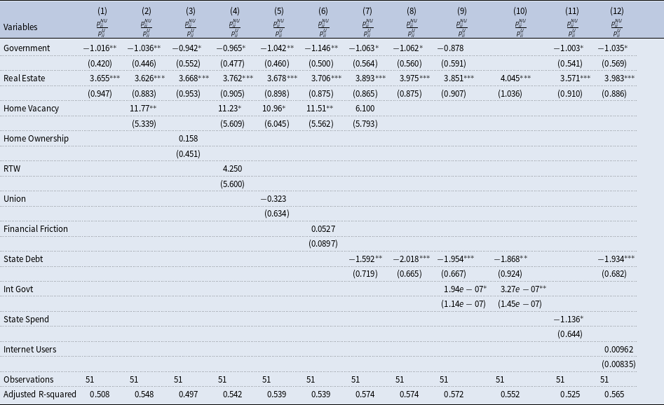
Notes: $\frac{p^{NU}_{ii}}{p^U_{ii}}$
is defined in Section 4.4 and represents the relative importance of national uncertainty shocks in propagating uncertainty shocks. White-corrected standard errors are in parentheses
$\frac{p^{NU}_{ii}}{p^U_{ii}}$
is defined in Section 4.4 and represents the relative importance of national uncertainty shocks in propagating uncertainty shocks. White-corrected standard errors are in parentheses $^{***}p\lt 0.01$
,
$^{***}p\lt 0.01$
, $^{**}p\lt 0.05$
,
$^{**}p\lt 0.05$
, $^{*}p\lt 0.1$
.
$^{*}p\lt 0.1$
.
Table 5 Column 1 presents our benchmark regression result from the first sequence of regressions relating the estimated responses $\rho _{i}$
to variables accounting for the structure of industry in each state where only the remaining significant industry variables are reported.Footnote
22
The column shows that only the share of the manufacturing and the mining industry have a robust and significant relationship with the responses of unemployment rate to an increase in US-wide uncertainty. These findings on the industry mix are completely consistent with those reported in Mumtaz et al. (Reference Mumtaz, Sunder-Plassmann and Theophilopoulou2018). We find that states with a higher concentration of the manufacturing industry experience a larger increase in unemployment after an increase in US-wide uncertainty. While speculative, this is consistent with the precautionary saving channel of uncertainty shocks causing a reduction in demand for manufacturing goods. On the other hand, we find that states with a larger mining industry experience a relatively smaller increase in unemployment. As documented in many studies such as Jo (Reference Jo2014), Mumtaz et al. (Reference Mumtaz, Sunder-Plassmann and Theophilopoulou2018) or Tran (Reference Tran2021), for instance, there is evidence that an uncertainty shock results in an increase in the price of some commodities. If this is the case, then the increase in commodity prices could be a contributing factor in negating the negative effects of uncertainty in states with a higher mining share of industry.
$\rho _{i}$
to variables accounting for the structure of industry in each state where only the remaining significant industry variables are reported.Footnote
22
The column shows that only the share of the manufacturing and the mining industry have a robust and significant relationship with the responses of unemployment rate to an increase in US-wide uncertainty. These findings on the industry mix are completely consistent with those reported in Mumtaz et al. (Reference Mumtaz, Sunder-Plassmann and Theophilopoulou2018). We find that states with a higher concentration of the manufacturing industry experience a larger increase in unemployment after an increase in US-wide uncertainty. While speculative, this is consistent with the precautionary saving channel of uncertainty shocks causing a reduction in demand for manufacturing goods. On the other hand, we find that states with a larger mining industry experience a relatively smaller increase in unemployment. As documented in many studies such as Jo (Reference Jo2014), Mumtaz et al. (Reference Mumtaz, Sunder-Plassmann and Theophilopoulou2018) or Tran (Reference Tran2021), for instance, there is evidence that an uncertainty shock results in an increase in the price of some commodities. If this is the case, then the increase in commodity prices could be a contributing factor in negating the negative effects of uncertainty in states with a higher mining share of industry.
Column 2 and Column 3 of Table 5 show that the variables reflecting the housing market (Home Vacancy or Home Ownership) are not significant and are thus excluded from the subsequent regression specifications. Columns 4–10 present the results of sequentially including variables reflecting: labor market conditions (i.e. Right to Work or Union Membership); financial conditions; and the fiscal condition (state-level debt, state-level spending, and intergovernmental transfers). We find that none of these variables exhibit a statistically significant relationship with the responses of unemployment to state-level uncertainty—with Manufacturing and Mining still remaining significant in most of these regressions. There is good evidence, therefore, to support the results reported in Column 1. Findings from these subsequent regressions (Column 2 onward), however, are in contrast to the results in Mumtaz et al. (Reference Mumtaz, Sunder-Plassmann and Theophilopoulou2018) who report a significant association between the effect of uncertainty and the state-level housing market, the fiscal condition, and the financial constraint. The difference in findings could be due to differences in the sample period (Mumtaz et al. (Reference Mumtaz, Sunder-Plassmann and Theophilopoulou2018) cover the period 1960Q1–2014Q1) and also the fact that the authors study the response of quarterly real income growth to an uncertainty shock. When we use unemployment as a measure of real economic activity and in a framework accommodating state interactions and feedbacks, the relationship between these variables and uncertainty shocks is weaker.
In summary, the benchmark estimates and the detailed robustness checks suggest the following results. First, states with a higher concentration of the manufacturing industry experience a larger increase in unemployment when impacted by an uncertainty shock. Second, states with a higher concentration of the mining industry appear to be affected less by this shock.
5.2 Heterogeneity of National Influences in the Propagation of Uncertainty Shocks
In this section, we employ the same regression and testing strategy as described in the previous section, with the dependent variable now $\rho _{i}=\frac{p_{ii}^{NU}}{p_{ii}^{U}}.$
Again, starting with a set of sequential regressions involving the first set of variables reflecting the industry structure (and as detailed in the Appendix), we end up with an industry mix involving Government and Real Estate remaining as the significant variables as the initial baseline regression and as reported in Column 1 of Table 6. To this baseline regression, we add Home Vacancy in Column 2 and Home Ownership in Column 3. Given the statistical significance of Home Vacancy, we keep it in the regression specification and add in sequentially Right to Work in Column 4, Union membership in Column 5, and the degree of financial frictions in Column 6. None of these latter three variables prove to be statistically significant. Home Vacancy also drops out with the inclusion of the measure of state-level debt.Footnote
23
We subsequently add in a measure of intergovernmental transfers as reported in Column 9. Although we find that the measure of intergovernmental transfers is statistically significant, we exclude this variable from the regression on the grounds that it takes on a value of almost 0, reduces the overall goodness-of-fit of the model as seen by the adjusted
$\rho _{i}=\frac{p_{ii}^{NU}}{p_{ii}^{U}}.$
Again, starting with a set of sequential regressions involving the first set of variables reflecting the industry structure (and as detailed in the Appendix), we end up with an industry mix involving Government and Real Estate remaining as the significant variables as the initial baseline regression and as reported in Column 1 of Table 6. To this baseline regression, we add Home Vacancy in Column 2 and Home Ownership in Column 3. Given the statistical significance of Home Vacancy, we keep it in the regression specification and add in sequentially Right to Work in Column 4, Union membership in Column 5, and the degree of financial frictions in Column 6. None of these latter three variables prove to be statistically significant. Home Vacancy also drops out with the inclusion of the measure of state-level debt.Footnote
23
We subsequently add in a measure of intergovernmental transfers as reported in Column 9. Although we find that the measure of intergovernmental transfers is statistically significant, we exclude this variable from the regression on the grounds that it takes on a value of almost 0, reduces the overall goodness-of-fit of the model as seen by the adjusted $R^{2}$
measure in Columns 8–10, and its inclusion takes away from the significance of the share of the government sector which has been a robust explanatory variable in all the other regressions.
$R^{2}$
measure in Columns 8–10, and its inclusion takes away from the significance of the share of the government sector which has been a robust explanatory variable in all the other regressions.
Our preferred specification is as in Column 8. The results in this column shows that only the government sector, the real estate industry, and the state-level of fiscal conditions are robust in terms of statistical significance in terms of the association the relative importance of the national influences in propagating uncertainty shocks. We find that states with a higher concentration of the real estate industry reflect a tendency for a state to experience a larger impact through national influences in propagating uncertainty shocks. The finding of the relatively greater importance of the national factors is consistent an increased degree of contagion between the financial market and the real estate market during the GFC, reflecting the housing bubble and the subprime mortgage lending crisis [Caporin et al. (Reference Caporin, Gupta and Ravazzolo2021)].
On the other hand, states with a more active fiscal policy experience less of an influence from the national factors in the propagation of uncertainty shocks. We find a negative and statistically significant relationship between the importance of national influences in propagating uncertainty shocks and the share of the government sector and the size of the state-level debt. Our conjecture on the negative association between an active fiscal policy and the importance of national influences in propagating uncertainty shocks is further solidified when we replace state-level debt by state-level spending in Table 6 Column 11. We find that there is a significant association between state-level spending and the importance of national factors in the propagation of uncertainty shocks. Finally, the inclusion of the share of internet users in Column 12 does not affect the results of our preferred specification.
In summary, the results from our preferred regression specification and detailed robustness checks suggest the following: the relative importance of national factors in the propagation of uncertainty shocks tends to be (i) smaller in states with a more active fiscal policy and (ii) greater in states with a larger concentration of the real estate industry.
6. Conclusion
Economic uncertainty is a salient and increasingly complex feature of the global economy. Therefore, it is important to understand how it can be better incorporated into macroeconomic models. One key and underexplored aspect is the role of spatial disaggregation, since local areas can differ greatly in their economic composition and therefore in their transmission mechanisms. This paper estimates the impact of uncertainty shocks in a disaggregate model featuring US state-level economic activity and uncertainty proxies, where internet search data is used as proxies for uncertainty. The disaggregate framework of analysis is in the context of the GVAR model which is able to characterize the evolution of state-specific variables while incorporating interactions and spillover effects across states.
We find there is strong evidence to support the usefulness of disaggregated data in models of uncertainty and economic activity for the USA, based on the ability of the disaggregate model to predict aggregate uncertainty and unemployment. The use of a disaggregate model accommodates and captures relevant feedbacks and interactions in the analysis on the impact of uncertainty on the economy—which the misspecified aggregate model omits. As a result, the disaggregate model exhibits significantly smaller effects of uncertainty shocks on the economy with a far more prolonged dissemination of these shocks compared to the aggregate model.
There is a large degree of heterogeneity across states in the respective responses of unemployment to a national uncertainty shock and also in the respective importance of national influences in propagating uncertainty shocks. Cross-sectional regression results suggest that the responses of unemployment are positively associated with the share of the manufacturing industry and negatively associated with the concentration of the mining industry. We also find that national influences are relatively less important than the state-specific influences in propagating the effect of uncertainty shocks and found to be positively associated with the size of the real estate industry and negatively associated with states exhibiting a more active fiscal policy, a greater share of the government sector, and higher levels of debt and spending. Further analysis on providing an economic commentary on the mechanisms underlying these results is certainly warranted and could provide important insights in informing state and national policies to mitigate the negative effects of uncertainty on the economy.


 Open access