2. Experiments

We show the experimental set-up in figure 1. We use a Taylor–Couette cell whose inner and outer radii are $R_{I} = 4\,\text {cm}$ and $R_{O} = 9\,\text {cm}$, respectively. The inner cylinder is stationary whereas the outer cylinder rotates at a constant angular velocity $\varOmega$.By construction, the flow is also stable with respect to centrifugal instability (Chandrasekhar Reference Chandrasekhar1961) and is therefore laminar. This configuration gives rise to an azimuthal velocity profile in the radial direction, $V_{\theta }(r) = Ar + B/r$ (with $A = \varOmega R_{O} / (R_{O}^{2} - R_{I}^{2})$ and $B = - \varOmega R_{O}R_{I}^{2} / (R_{O}^{2} - R_{I}^{2})$). As the settling lamella has initial (and hence maximum) width $s_{0} \simeq 2.5 \times 10^{-3}\,\text {m} \ll R_{O} - R_{I}$, it experiences a flow with constant (radial) shear rate $\gamma := r \partial _{r}[V_{\theta }/r] \rvert _{r = R_{b}} = -2B/R_{b}^{2}$ (where $R_{b}$ is the radial position at which the blob is deposited), independent of the vertical coordinate $z$. We fill the cell with two-thirds glycerol and one-third linearly stratified salt water (as shown in figure 1a) using the double-bucket method, creating a stratification characterised with a buoyancy frequency of $N^{2} \simeq 1.4\,\text {s}^{-2}$.

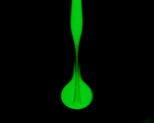
Figure 1. (a) Typical ambient density profile: crosses correspond to experimental measurements; the solid line corresponds to a linear fit. (a,b) Experimental set-up: a (green) blob of density $\rho _{0}$ is released at the surface of the cell, experiencing a local azimuthal velocity radial shear rate $\gamma$. The distance $z_{0}$ is the distance from the surface to the location where the ambient density is $\rho _0$. The inset of (b) shows a reconstruction corresponding to an iso-concentration surface, defining the lamella's time-dependent length $\ell$ and width $\eta \ll \ell$. This reconstruction consists of multiple frames as the lamella rotates through the laser sheet. (c) Top (offset) views of the settling lamella at five different times (separated by a rotation period; an artificial shift in the $y$-direction has been added between each frame), showing $\ell (t)$ to increase approximately linearly (red dashed lines).

The stratification suppresses any significant Ekman pumping during an individual experiment, while the kinematic viscosity of the experimental fluid, $\nu = 2.6 \times 10^{-5}\,\text {m}^{2}\,\text {s}^{-1}$, ensures that the Reynolds number ${Re} \lesssim 10^{-1}$, preventing all potential flow instabilities (without glycerol the initial blob quickly transforms into a vortex ring that destabilises through Rayleigh–Taylor-type instabilities and then disintegrates; these are the kinds of instabilities that we aim to damp using a more viscous fluid). The viscosity of the water–glycerol mixture is estimated using parametrisations developed by Cheng (Reference Cheng2008) and Volk & Kähler (Reference Volk and Kähler2018). The molecular diffusivity $D$ of salt in this mixture is estimated using the Stokes–Einstein formula and found to be $D \simeq 3.7 \times 10^{-11}\,\text {m}^{2}\,\text {s}^{-1}$, so that ${Pr} \simeq 7.0 \times 10^{5}$.

We prepare a blob (using the same mixture) to have density $\rho _{0} (=1.217\,\text {g}\,\text {cm}^{-3})$, corresponding to the background density $\bar {\rho }$ at the height defined as $z=0$, located approximately $0.5H$ above the bottom of the container to prevent interactions with the bottom boundary. We form the initial blob at the tip of a syringe that is gently brought towards the surface of the cell. As soon as the blob touches the surface, it is injected into the liquid bulk by the release of surface tension stresses and slowly falls down due to buoyancy forces, as the surface is a distance $z=z_0$ above the location where $\bar {\rho }=\rho _0$. We dye the blob using fluorescein. The molecular diffusivity of the fluorescein in the salt-water–glycerol mixture is estimated to be of order $D_{fluo} \simeq 1.6 \times 10^{-10}\,\text {m}^{2}\,\text {s}^{-1}$, so $(D/D_{fluo})^{1/3} \simeq 0.6$, implying that the evolution of fluorescein concentration is a good proxy for tracking the evolution of salt concentration and hence density in the settling lamella.

We visualise the settling lamella through laser-induced fluorescence of fluorescein using a fixed vertical blue laser sheet (in the $x$–$z$ plane, perpendicular to the flow) that the lamella crosses as it falls. The data are acquired using a low-light-sensitive camera appropriately calibrated (see Meunier Reference Meunier2020). The set-up has a spatial resolution of $2.0 \times 10^{-5} \,\text {m}\,\text {pixels}^{-1}$, which ensures that the key Batchelor scale $\eta _{B} \simeq s_0 {Pe}^{-1/3}$ (see e.g. Souzy et al. Reference Souzy, Zaier, Lhuissier, Le Borgne and Metzger2018) is resolved for the range of parameters studied here, $\eta _{B} \in [5\times 10^{-5}\,\text {m},\ 9\times 10^{-5}\,\text {m}]$.

Figure 1(c) presents (offset) top-view visualisations of the blob when it is stretched by the shear, showing that the length $\ell (t)$ of the blob increases approximately linearly at late times, as determined through the kinematics (for a constant shear rate $\gamma$) by

(2.1)\begin{equation} \ell = s_0\sqrt{1 + (\gamma t)^{2}}. \end{equation}

Figure 2 shows qualitatively the vertical trajectory of a blob as it settles for various shear rates $\gamma$, associated with different rotation rates $\varOmega$. In the absence of shear, the blob falls down until its position $z_b$ actually reaches $z=0$, where its (initial, unmixed) density $\rho _0$ is equal to the background density $\bar {\rho }(z=0)$ (figure 2a). The main blob is followed by a thin filament reorganising into small secondary blobs, which will not be considered in this paper. This might be the consequence of a Rayleigh–Plateau-type instability, the fluorescein potentially changing the surface tension of the fluid in the settling blob. The (unsheared) blob also seems to start forming a dense-core vortex ring, as can be seen for instance in the middle section of figure 2(a). Such a structure is known to enhance mixing with the surrounding fluid, as discussed in Linden (Reference Linden1973), Camassa et al. (Reference Camassa, Khatri, McLaughlin, Mertens, Nenon, Smith and Viotti2013) and Olsthoorn & Dalziel (Reference Olsthoorn and Dalziel2017) in the case of strongly stratified interfaces, but this effect was not seen here, at least within the precision of our measurements, viscosity potentially preventing the full development of the vortex ring. In the presence of shear ($\varOmega \neq 0$), the width $\eta$ of the blob decreases at early times since the blob is stretched in the along-lamella direction. The drag is therefore higher and diffusion acts sooner, thus reducing the (driving) buoyancy force. As a consequence, the blob falls more slowly, mixes with the surrounding (less dense) fluid and hence stops before reaching $z=0$. This effect is clearly visible in figure 3(a), showing the temporal evolution of the vertical position of the blob. Quantitatively, the final position of the lamella, denoted by $z_f$, increases from $0.1 z_0$ to $0.7 z_0$ when the shear increases from $0.1$ to $1\,\mathrm {s}^{-1}$.

Figure 2. (a–c) Settling of a dyed lamella of initial density $\rho _0$ released at the surface for different rotation speeds $\varOmega$ of the outer cylinder. The height $z_{0}$ corresponds to the vertical distance between the surface and the position $z=0$ where the ambient density $\bar {\rho }=\rho _0$. Note that in the sheared cases, the blob initially split into a main and a secondary blob. The discussion that follows and the model developed in this work for the settling dynamics of the blob focus on the main blob (framed in red), which does not lose mass except through a weak trailing filament, and we will hence use its total mass as the conserved mass in our model (see § 3).

Figure 3. (a) Experimental and theoretical (from (3.4)) vertical trajectories of the settling lamellae for various rotation speeds $\varOmega$. The position of the blob is scaled by $z_{0}$ and time is scaled by the mixing time $t_{S} = \gamma ^{-1}{Pe}^{1/3}$ (in dimensional form). The thick black line corresponds to a numerical integration of (3.4). The dotted black line corresponds to the non-diffusive model (3.7). The dashed black line corresponds to the non-diffusive model (3.7) settled at $t=t_{S}$. Note that the data are collected when the maximal concentration point of the lamella crosses the laser sheet, i.e. once per rotation period of the lamella around the set-up, and not continuously. (b) Dimensionless final position of the settling lamella for various shear rates $\gamma$. The data are also presented as a function of ${Re}/{Fr}^{2}$, a parameter that controls the mixing criterion developed in § 3.3. The dashed black line corresponds to the approximation given by (3.10), whereas the thick black line corresponds to a numerical integration of (3.4). The shaded region corresponds to the range of shear rates $\gamma$ for which the lamella settles at $z_f \simeq 0$, i.e. its final density is approximately unchanged.

3. Model for a mixing lamella

We develop a simple model coupling the vertical motion of a settling lamella with its mixing dynamics and then discuss its implications for mixing more generally. We formulate a time-dependent force balance where $F_{D}(t)$ is the drag force, $F_{B}(t)$ the buoyancy force, $\rho _b(t)$ the density of the lamella, $V_b(t)$ its volume and $z_{b}(t)$ its vertical position:

(3.1)\begin{equation} \rho_b V_b\frac{\mathrm{d}^{2}z_{b}}{\mathrm{d}t^2} = F_{D} + F_{B}, \end{equation}

where

(3.2a,b)\begin{equation} F_{B} ={-} \left[\rho_b - \bar{\rho} (z_{b})\right] V_{b}(t) g,\quad \bar{\rho}(z) = \rho_{0} \left( 1-\frac{N^2}{g}z \right) \end{equation}

and $N$ is the (constant) buoyancy frequency. The settling velocity $\mathrm {d}{z_b}/\mathrm {d}t$ ensures that the Reynolds number of the wake $|\mathrm {d}{z_b}/\mathrm {d}t|\eta /\nu \lesssim O (10^{-3})$. In this Stokes regime, the drag force is proportional to the settling velocity and the length of the lamella $\ell (t)$:

(3.3)\begin{equation} F_{D} ={-}\frac{\rm \pi}{6} \alpha \nu \rho_{0} \ell(t) \frac{\mathrm{d}z_{b}}{\mathrm{d}t} \end{equation}

using the Boussinesq approximation, fixing the density at the reference value $\rho _0$. The drag coefficient $\alpha$ depends on different parameters of the problem such as the viscosity of the fluid, the settling speed of the lamella and its geometry. It has been taken to be approximately $7$, a value that gives good agreement between the experimental data and the theoretical predictions (see figure 3a). This value of $\alpha$ can be compared with its theoretical value computed assuming that the lamella is an infinite cylinder of radius $s_{0}$ settling at a constant speed $U$ (see e.g. Lamb Reference Lamb1932), $\alpha _{th} = 24 / [(1/2) - \gamma _{E} - \log (Us_{0}/4\nu )] \simeq 5$ where $U = O (10^{-3})\,\text {m}\,\text {s}^{-1}$ is the mean vertical velocity of the settling lamella and $\gamma _{E}$ is Euler's constant. A better drag model (especially for low shear rates $\gamma \ll 1$) would perhaps consist of a finite-volume drag model for spheroids (that importantly evolves as the shape of the lamella changes) such as that developed by Chwang & Wu (Reference Chwang and Wu1975). For the sake of simplicity, we did not investigate this option further.

Mass conservation ensures that $\rho _b V_b = \rho _{0} V_{0}$ where $V_{0}={\rm \pi} s_0^3/6$ is the initial volume of the (assumed spherical) blob. Note that in the sheared cases, the blob initially (more precisely, before the first passage of the blob through the laser sheet, i.e. within one half-rotation period) split into a main and a secondary blob. The discussion that follows and the model developed here focus on the main blob (highlighted in red in figure 2), which does not lose mass except through a weak trailing filament and for which mass conservation thus seems to be valid. Note that we can reconstruct the main blob using multiple images as it rotates through the laser sheet and hence estimate its volume. Using this technique for the second and third passages of the lamella at $\varOmega = 8\,\text {r.p.m.}$ (experiment presented in figure 2b), we find that, within the error bounds of the method, the volume of the lamella is conserved and is approximately $3\times 10^{-9}\,\text {m}^{3}$. Since these measurements are done before the mixing time (estimated to be $169\,\text {s}$ in this particular case), this further supports that conservation of mass is valid for the main blob within the approximations done in this work. Hence, we focus here on the main blob and use its total mass as the conserved mass in our model.

We now non-dimensionalise all quantities using the initial size of the blob $s_0$ and the shear rate $\gamma$ so that $\hat {z}_b\equiv z_b/s_0$, $\hat {z}_{0} \equiv z_{b}/s_{0}$, $\hat {t}\equiv \gamma t$, $\hat {\rho }_b\equiv \rho _b/\rho _0$, $\hat {N}\equiv N/\gamma$, $\hat {V}_b\equiv V_b/V_0$ and $\hat {\ell }\equiv \ell /s_0$, and we obtain

(3.4)\begin{equation} \frac{\mathrm{d}^2\hat{z}_{b}}{\mathrm{d}\hat{t}^2} ={-} \frac{\alpha}{Re}\hat{\ell}\frac{\mathrm{d}{\hat{z}_{b}}}{\mathrm{d}\hat{t}} - \left(\frac{1}{{Fr}^2\hat{\rho}_b} \right ) \hat{z}_{b} - \beta\left(1 - \frac{1}{\hat{\rho}_b}\right) \quad \textrm{with}\ \hat{\ell}= \sqrt{1 + \hat{t}^{2}}, \end{equation}

where

(3.5a–c)\begin{equation} {Re} := \frac{\gamma s_0^2}{\nu},\quad {Fr} := \frac{\gamma}{N},\quad \beta := \frac{g}{s_{0}\gamma^2}. \end{equation}

Here ${Fr}$ is a Froude number that compares the buoyancy time scale $1/N$ to the shear time $\gamma ^{-1}$, while the parameter $\beta$ compares the inviscid free-fall time $\sqrt {s_{0}/g}$ to the shear time. For $\gamma = 0.1\,\text {s}^{-1}$, we have ${Re} \simeq 10^{-2}$, ${Fr}^2 \simeq 10^{-1}$, $\beta \simeq 10^{4}$ and ${Pe} \simeq 10^{4}$. For $\gamma = 1\,\text {s}^{-1}$, we have ${Re}\simeq 10^{-1}$, ${Fr}^2 \simeq 10$, $\beta \simeq 10^{2}$ and ${Pe} \simeq 10^{5}$. Thus, this experiment can access weakly stratified (high ${Fr}$) and strongly stratified (low ${Fr}$) laminar flow regimes, at large ${Pe}$. Note that another important dimensionless parameter of our system is the Archimedes number (comparing buoyancy and viscous forces), defined as

(3.6)\begin{equation} {Ar} := \frac{gs_{0}^{3}\left[\rho_{0} - \bar{\rho}(z_{0})\right] / \bar{\rho}(z_{0})}{\nu^{2}}, \end{equation}

where $\bar {\rho }(z_{0})$ is the density of the surrounding fluid at the injection point. The Archimedes number was estimated to be approximately $4$. In the rest of the paper, we will work with dimensionless quantities (unless otherwise stated) and will therefore drop the hats for clarity.

3.1. Non-diffusive dynamics

Given the low values of ${Re} \ll 1$, the settling dynamics is over-damped, so inertia can be neglected in (3.4) (i.e. $\mathrm {d}^{2}{z_b}/\mathrm {d}t^2 \simeq 0$). Considering the initial regime when the deforming lamella has not yet mixed and its density is still unaltered (i.e. dimensionless $\rho _b=1$),

(3.7)\begin{equation} z_{b}(t) = z_0 \left[\sqrt{1 + t^{2}} + t\right]^{-{Re}/(\alpha {Fr}^2)}. \end{equation}

We plot this prediction in figure 3(a) (dotted lines). Unlike in the experiment, (3.7) predicts that $z_b \rightarrow 0$ as $t\rightarrow \infty$. Indeed, in the absence of diffusion the blob is always denser than the surrounding fluid for $z_b>0$. We thus need to introduce diffusive effects to predict the final position correctly.

3.2. Diffusive dynamics

Figure 4(a) shows the temporal evolution of the maximal dye concentration $C_{\textit{max}}$ and the corresponding blob width. The shear stretches the blob into a thin lamella, enhancing diffusion and leading to a decrease of the maximal concentration. We know that for the linear stretching stirring protocol studied here, the diffusion problem (and hence the maximal concentration) depends on the Ranz time $\tau$ (Ranz Reference Ranz1979; Villermaux Reference Villermaux2019):

(3.8)\begin{equation} C_{max}=C_0\, \text{erf}\left[\frac{1}{4\sqrt{\tau}}\right],\quad \text{where}\ \tau = \frac{1}{Pe} \int \ell(t)^2 \,\mathrm{d}t =\frac{1}{Pe}\left[t + \frac{t^3}{3}\right] \end{equation}

and $C_{0}$ is the initial concentration of dye in the blob. We plot this prediction with solid lines in figure 4(a). There is excellent agreement with the experimental measurements even though the prediction ignores dynamic buoyancy effects.

Figure 4. (a) Time evolution of the scaled concentration of dye and (b) scaled width of the settling lamella. Time is scaled using the mixing time $t_{S} = \gamma ^{-1}{Pe}^{1/3}$ (in dimensional form). The solid lines correspond to the theoretical predictions (3.8) and (3.9). The size of the symbol in (b) is larger than in (a) to take into account the fact that measurements of the lamella's width are more prone to errors, especially as we approach the Batchelor width. Note that the data are collected when the maximal concentration point of the lamella crosses the laser sheet, i.e. once per rotation period of the lamella around the set-up, and not continuously.

The diffusive width of the lamella is equal to the Batchelor thickness given by (see Souzy et al. Reference Souzy, Zaier, Lhuissier, Le Borgne and Metzger2018; Villermaux Reference Villermaux2019)

(3.9)\begin{equation} \eta = \frac{1}{\ell} \sqrt{1+4\tau} = \sqrt{\frac{1+4(t+t^3/3)/{Pe}}{1 + t^2}}. \end{equation}

As shown in figure 4(b), $\eta$ decreases initially and then increases as $\sqrt {t}$ when diffusion becomes efficient. Hence, mixing starts when $\tau > 1$, i.e. when (in dimensionless form)$t > t_{S}$ where $t_{S}={Pe}^{1/3}$. Interestingly, the equilibrium position is reached at approximately the same mixing time $t=t_{S}$ as shown in figure 3(a). This is because the difference between the lamella's density and the surrounding fluid's density suddenly decreases at $t=t_S$, thus cancelling out the buoyancy force and stopping the descent of the blob. As a first approximation, we can assume that the final position $z_{f}$ of the settling lamella (formally equal to $z_{b}(t \rightarrow \infty )$ where diffusion has been taken into account) is approximated by its predicted position in the absence of diffusion, (3.7), at $t=t_{S}$:

(3.10)\begin{equation} z_f \simeq z_{b}(t_{S}) = z_{0}\left[\sqrt{1 + {Pe}^{2/3}} + {Pe}^{1/3}\right]^{-{Re}/(\alpha{Fr}^{2})}. \end{equation}

We compare this theoretical prediction with experimental data in figure 3(b). The prediction slightly overestimates the equilibrium position. Indeed, the lamella does not abruptly stop at the mixing time. However, there is reasonable agreement in both magnitude and trend.

To improve this prediction, we now assume that the (dimensional) density of the lamella $\rho _b(t)$ decreases towards the density of the surrounding fluid $\bar {\rho }$ with the same temporal dependence as the maximal concentration, i.e. that for $t< t_{S}$ the density of the lamella remains relatively constant but converges towards the density of the surrounding fluid for $t>t_{S}$. In other words, we assume, using dimensional quantities, that

(3.11)\begin{equation} \rho_b(t) - \bar{\rho}(z_{b})= \left[ \rho_b(0) - \bar{\rho}(z_{b})\right] \text{erf}\left[\frac{1}{4\sqrt{\tau}}\right]. \end{equation}

Rewriting $\bar {\rho }$ from (3.2a,b) in dimensionless form yields

(3.12)\begin{equation} \rho_b(t) = 1 - \frac{1}{\beta{Fr}^{2}}z_{b} + \frac{1}{\beta {Fr}^{2}}z_{b}\,\text{erf}\left[\frac{1}{4\sqrt{\tau}}\right]. \end{equation}

Using this expression for the lamella's time-dependent density, the trajectory of the lamella can no longer be derived theoretically from (3.4). We solve the system numerically using a backward differentiation method with adaptive time-stepping and plot solutions for various values of the shear rate $\gamma$ in figure 3(a) (solid lines), demonstrating excellent agreement with the overall time evolution of the vertical trajectory of the blob.

3.3. Implications for mixing

The final density of the lamella, and hence the relative amount of mixing it has experienced, can be inferred from the lamella's equilibrium position. The closer the equilibrium position is to its initial position $z_0$, the more the lamella has mixed with the surrounding fluid. In that sense, $z_f/z_{0}$ in its dimensionless form may be interpreted as a ‘mixing efficiency’, particularly as it is exactly equal to the ratio between the increase of the background potential energy and the available potential energy of the initial blob, even though the only dynamic effect of the buoyancy has been on the (inertialess) settling of the lamella.

For the linear stretching considered here using (3.10), efficient mixing ($z_f \simeq z_0$) requires

(3.13)\begin{equation} \frac{{Re}\ln({Pe})}{{Fr}^{2}} \ll 3 \alpha = O (10). \end{equation}

This mixing criterion incorporates all the effects involved in the problem. A strong stratification (large $N$) must be compensated for by a large shear $\gamma$ to meet a given efficiency (i.e. keeping ${Fr}$ fixed). Viscous damping (large $\nu$) will actually slow down settling and favour efficiency. Significantly, weak diffusion (small $D$ and hence larger ${Pe}$) will delay mixing, thus reducing efficiency (consistent with simulations as discussed in the Introduction), although through a weak, but nevertheless quantifiable, logarithmic correction, as is classically the case for all stretching-enhanced diffusion processes (Villermaux Reference Villermaux2019).

3.4. Generalisation

The above results are valid for a linear shear (i.e. $\ell (t) \sim t$ at large times), but are readily generalised to any stretching flow. For a given $\ell (t)$, from (3.4), for times $t \leq t_{S}$ we can obtain the general expression (in the absence of diffusion and in the ${Re} \ll 1$ regime)

(3.14)\begin{equation} z_{b}(t)= z_0 \exp\left[ -\frac{Re}{\alpha{Fr}^{2}} \int_{0}^{t}\frac{\mathrm{d}t'}{\ell(t')} \right]. \end{equation}

For example, if the lamella is exponentially stretched so that $\ell (t)= \text {e}^{t}$, the position $z_b (t_S)$ is

(3.15)\begin{equation} z_f \simeq z_{b}(t_{S}) = z_0 \exp\left[-\frac{Re}{\alpha{Fr}^{2}} \left(1 -\frac{1}{\sqrt{Pe}}\right)\right] \end{equation}

since the mixing time $t_{S} = \ln ({Pe})/2$ (Batchelor Reference Batchelor1959; Villermaux Reference Villermaux2019) in that case. Although consistent with the linear stretching case ($z_f$, and hence the efficiency, monotonically decreases as ${Pr}$ increases), the final position converges to a finite value $z_0 \exp [-{Re}/(\alpha {Fr}^2)]$ in the limit ${Pe} \rightarrow \infty$. Perhaps surprisingly, the blob does not reach $z=0$ as $D \rightarrow 0$ since the drag increases so rapidly. Very interestingly, (3.15) demonstrates that when the elongation is sufficiently rapid (exponential), the final equilibrium position $z_f$ is independent of the Péclet number ${Pe}$ as ${Pe} \rightarrow \infty$, since the analogue of the criterion (3.13), remaining valid as $D \rightarrow 0$, is

(3.16)\begin{equation} \frac{Re}{{Fr}^{2}} \ll \alpha = O (10). \end{equation}

This result, arising from a deterministic, smooth, non-singular stirring process, has a significant implication for scalar dissipation cascades. A classical ‘law’ of passive scalar turbulence is that $D\lvert \boldsymbol {\nabla } C\rvert ^2$, where C is the concentration of the scalar, remains finite as $D\to 0$. Although some counter-examples to this law have been presented (see for example Balmforth & Young Reference Balmforth and Young2003), a consistent argument for when this law applies in passive scalar mixing can be formulated (Villermaux Reference Villermaux2012, Reference Villermaux2019). Essentially, the (finite) mixing time $t_{S}$ is independent of $D$ only when $\ell (t)$ diverges in a finite time $t_\star =t_{S}$. In the stratified situation considered here, this condition on $\ell (t)$ is relaxed. As there is an inherent coupling between the lamella settling speed and its density, there is a slowing cascade towards immobility. During this cascade (which does not terminate in finite time) diffusion can disappear, even though diffusion is the actual mechanism driving the density equalisation. There is a highly suggestive analogy with the way that viscosity disappears in the infinitely accelerating cascade towards viscous dissipation in the kinetic energy cascade (Donzis, Sreenivasan & Yeung Reference Donzis, Sreenivasan and Yeung2005), leading to the ‘zeroth law of turbulence’.