

1. INTRODUCTION
The Global Navigation Satellite Systems (GNSS) can provide real-time Position and Velocity (PV) information suitable for most land, marine, and aircraft navigation applications (Parkinson and Spilker Reference Parkinson and Spilker1996). In GNSS kinematic positioning and navigation, the pseudorange measurement is preferred to the carrier-phase measurement due to its exemption of unknown integer cycle. In general, the metre and sub-metre level kinematic solutions are achievable from the single point positioning and the differential GNSS technique, in real time respectively. As an effective and important complement to GNSS kinematic navigation, the GNSS Doppler measurements provide the velocity information of moving objects (Parkinson and Spilker Reference Parkinson and Spilker1996; Bruton et al., Reference Bruton, Glennie and Schwarz1999; Zhang et al., Reference Zhang, Zhang, Grenfell and Deakin2006; Remondi, Reference Remondi2004; Zhou et al., Reference Zhou, Shen and Li2011). In GNSS kinematic navigation and positioning, it still faces many challenges due to, for instance, the signal degradation, the blockages and the colored noise etc. Extensive research efforts have been done towards optimizing the solution and maximizing the reliability in past two decades (Teunissen Reference Teunissen1990; Wang Reference Wang2000; Hewitson and Wang Reference Hewitson and Wang2007; Kuusniemi et al., Reference Kuusniemi, Lachapelle and Takala2004).
As an efficient implementation of the sequential least squares adjustment with relative constraints between-state, the Kalman Filter (KF) is extensively applied in the navigation computations assuming that the observational error and the prediction error are uncorrelated and both normally distributed with zero means (Brown and Hwang Reference Brown and Hwang1997; Simon, Reference Simon2006). In real applications, the unexpected errors inevitably exist in either the dynamic model or the observation model. Therefore, to balance the contributions of the observation and the prediction to the solution, the adaptive and robust filtering techniques were developed based on the robust M-estimation, optimal theory and Bayesian estimation (Koch and Yang Reference Koch and Yang1998; Yang et al., Reference Yang, He and Xu2001, Reference Yang and Xu2003, Reference Yang and Gao2005; Wang Reference Wang2000, Hewitson and Wang Reference Hewitson and Wang2007; Geng and Wang Reference Geng and Wang2008).
The KF approach relies, to a great extent, on the quality of dynamic model that describes the moving object's motion behaviour. In the existing literatures, the Constant Velocity (CV) and the Constant Acceleration (CA) dynamic models are popularly employed in navigation. However, the CV model is too simple to describe the motion detail and then suits only for those low-dynamic or high sampling rate systems. Although the CA model can capture the motion in more details, the acceleration cannot be directly obtained from the GNSS receivers. Furthermore, both two models would be problematic to describe the moving object's manoeuvring that is a complicated and unpredicted dynamic process. Thorp (Reference Thorp1973) proposed to model this dynamic process of manoeuvring as a stochastic departure from a nominated base trajectory to obtain the reasonable performances, while Singer (Reference Singer1970) solved for such dynamic process as a noisy component by using a known exponential auto-correlation acceleration function. In addition, an extended ‘Singer’ model was then developed permitting the time-correlation in both the velocity and the acceleration components (Moore and Wang Reference Moore and Wang2003). Another dynamic model based on ‘kinematic’ method was applied in KF, which introduces the variation of moving object's positions to reflect the mean velocity in two consecutive epochs (Schwarz et al., Reference Schwarz, Cannon and Wong1989).
These dynamic models aforementioned are established based on state of the previous one epoch only, which is impossible to provide the sufficient information for describing the moving object's motion characteristic of current epoch, thus leading to the increased degradation and instability risks in kinematic solutions. Therefore, it is necessary to include more historical information in the dynamic model. The Windowing-Recursive Approach (WRA) provides a new strategy to estimate the state of vehicles (Zhou et al., Reference Zhou, Shen and Li2010). Its basic principle is that the trajectory of a vehicle can be reasonably fitted by using the positions of latest several epochs in a short time span. Therefore the position at the current epoch can be predicted more reliably with the positions of the multiple historical epochs rather than the latest one epoch. In WRA, the dynamic model of vehicle is adaptively recovered in real time without any assumption on the dynamic characteristics, like CV model. The WRA is flexible and can reduce to KF if the window consists only of one epoch. However, in the first WRA literature of Zhou et al., (Reference Zhou, Shen and Li2010), the WRA was implemented with the GNSS pseudorange measurements and the efficient state transition matrix was constructed only for the case where the state vector consists only of three-dimensional position. Nevertheless, velocity needs to be estimated in real time besides position in most of GNSS navigation applications, such as aircrafts and missiles. Therefore, the implementation of WRA should be extended from the three-dimensional position state to the six-dimensional PV state to estimate the reliable and accurate real-time solutions by taking full advantages of velocity information. In this contribution, the implementation of WRA with six-dimensional PV state vector will be developed using the pseudorange and Doppler measurements. Its corresponding state transition matrix is constructed based on the Newton's Forward Difference Extrapolation (NFDE) and Definite Integral (DI) methods for the efficient computation.
The rest of paper is organized as follows. In Section 2, Kalman filtering and the WRA are introduced in brief. In Section 3, the implementation of WRA is developed based on the pseudoranges and Doppler measurements. In Section 4, we will construct the adaptive, efficient and practical state transition matrices for the proposed WRA implementation based on the NFDE and DI numerical methods. A real vehicular GNSS experiment is introduced in Section 5 to demonstrate the performance of the new WRA implementation. Finally, some concluding remarks are given in Section 6.
2. KALMAN FILTERING AND WINDOW-RECURSIVE APPROACH
2.1. Kalman Filtering
As an efficient realization of the sequential least-squares adjustment, the KF has been widely used in the GNSS navigation computations. A linear dynamic model and an observation model are involved in the KF:
 $${\bi x}_k = {\bi \Phi} _{k,k - 1} {\bi x}_{k - 1} + {\bi w}_k $$
 $${\bi l}_k = {\bi H}_k {\bi x}_k + {\bi \varepsilon} _k $$
where:
- The subscripts denote the epoch number.
- x is the state vector to be estimated.
- l is the measurement vector.
- w and ε are the process noise in dynamic model and the measurement noise with the zero means and the covariance matrices of Σ w and R, respectively.
- Φ is the state transition matrix that transfers the state vector from the (k − 1)th epoch to the kth epoch.
- H is the design matrix connecting the state vector with the observation vector.
The sequential formulae in KF are given:
 $${\bi \bar x}_k = {\bi \Phi} _{k,k - 1} {\bi \hat x}_{k - 1} $$
 $${\bi \Sigma} _{{\bi \bar x}_k} = {\bi \Phi} _{k,k - 1} {\bi \Sigma} _{{\bi \hat x}_{k - 1}} {\bi \Phi} _{K,k - 1}^T + {\bi \Sigma}_{{\bi w}_{k}} $$
 $${\bi K}_k = {\bi \Sigma} _{{\bi \bar x}_k} {\bi H}_k^T \left( {{\bi H}_k {\bi \Sigma} _{{\bi \bar x}_k} {\bi H}_k^T + {\bi R}_k} \right)^{ - 1} $$
 $${\bi \hat x}_k = {\bi \bar x}_k + {\bi K}_k \left( {{\bi l}_k - {\bi H}_k {\bi \bar x}_k} \right)$$
 $${\bi \Sigma} _{{\bi \hat x}_k} = \left( {{\bi I} - {\bi K}_k {\bi H}_k} \right){\bi \Sigma} _{{\bi \bar x}_k} $$
where:
- I is the identity matrix with same dimensions of ${\bi \Sigma} _{{\bi \bar x}_k} $.
 - ${\bi \bar x}_k $ ${\bi \Sigma} _{{\bi \bar x}_k} $ denotes the predicted state vector and its covariance matrix, respectively.
- Kk is the gain matrix. ${\bi \hat x}_k $ and ${\bi \Sigma} _{{\bi \hat x}_k} $ are the posterior KF estimate and its covariance matrix.


If the dynamic model or/and observation model is nonlinear, the Extended Kalman Filtering (EKF) would be applied where these nonlinear models are linearized (Brown and Hwang Reference Brown and Hwang1997; Simon Reference Simon2006). The EKF can be viewed as the conventional KF in the first-order approximated linear model. These approximations, however, may introduce the large errors in the true posterior mean and covariance of the transformed Gaussian Random Variable (GRV), resulting in the sub-optimal performance or even filtering divergence. To overcome the pitfalls of EKF, the sigma-points and Unscented Kalman Filtering (UKF) approaches were developed (Julier and Uhlmann Reference Julier and Uhlmann1997; Julier et al., Reference Julier, Uhlmann and Durrant-Whyte2000; Jwo and Lai Reference Jwo and Lai2009) and have been successfully applied in target tracking field. The state distribution is again represented by a GRV but specified by using a minimal set of carefully chosen sample points. These sampled points can adequately capture posterior mean and covariance accurately to the 3rd order (Taylor series expansion) for any nonlinearity when propagated through the true non-linear system. Since the nonlinearity of the GNSS observational model is so weak that we can basically neglect its influence on estimation accuracy, the EKF is preferable in GNSS navigation (Jwo and Lai Reference Jwo and Lai2008).
2.2 A Brief Review on Window-Recursive Approach
In traditional navigation applications, the dynamic model is established based on the state of the previous one epoch only, which is impossible to provide the sufficient information for describing the moving object's motion characteristics of current epoch, thus leading to the increased degradation and instability risks in kinematic solutions. To overcome this limitation, the WRA was proposed in Zhou et al., (Reference Zhou, Shen and Li2010). Its principle is that the position at the current epoch is predicted more reliably with the positions of the multiple historical epochs than with the position only of the latest epoch. Assuming that the time-window length contains n epochs, the dynamic model is constructed as:
 $${\bi x}_k = {\bi \Phi} _{\left( {k,k - n:k - 1} \right)} {\bi x}_{\left( {k - n:k - 1} \right)} + {\bi w}_k $$
where
- x(k − n:k − 1) is the vector consisting of the stacked state vectors from the epoch (k − n) to the epoch (k − 1).
- Φ(k ,k − n:k − 1) is the transition matrix that transfers the state information of the previous n epochs into that of the current one.
Let  ${\bi \Sigma} _{{\bi \hat x}_{\left( {k - n:k - 1} \right)}} $ be the covariance matrix of the historical state vector ${\bi \hat x}_{\left( {k - n:k - 1} \right)} $, the predicted position vector at epoch k and its corresponding covariance are derived:
 $${\bi \bar x}_k = {\bi \Phi} _{\left( {k,k - n:k - 1} \right)} {\bi \hat x}_{\left( {k - n:k - 1} \right)} $$
and:
 $${\bi \Sigma} _{{\bi \bar x}_k} = {\bi \Phi} _{\left( {k,k - n:k - 1} \right)} {\bi \Sigma} _{{\bi \hat x}_{\left( {k - n:k - 1} \right)}} {\bi \Phi} _{\left( {k,k - n:k - 1} \right)}^T + {\bi \Sigma} _{{\bi w}_k} $$
respectively.
In the linear(ised) observation Equation (1b) at epoch k, the covariance matrix of measurements is expressed as Rk=σ 02Pk−1. Here, σ 02 is a known prior variance scalar and Pk is a weight matrix. By minimizing the weighted quadratic measurement residual vector  ${\bi v}_k = {\bi H}_k {\bi \hat x}_k - {\bi l}_k $ and the weighted quadratic predicted residual vector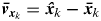 ${\bi \bar v}_{{\bi x}_k} = {\bi \hat x}_k - {\bi \bar x}_k $, the Bayesian risk function is established by:
 $$\mathop {\min} \limits_{{\bi x}_k} :{\bi v}_k^T {\bi P}_k {\bi v}_k + {\bi \bar v}_{{\bi \bar x}_k} ^T {\bi P}_{{\bi \bar x}_k} {\bi \bar v}_{{\bi \bar x}_k} $$
where  ${\bi P}_{{\bi \bar x}_k} = \sigma _0^2 {\bi \Sigma} _{{\bi \bar x}_k} ^{ - 1} $ denotes the weight matrix of the predicted state vector.
The solution of minimization problem Equation (6) is:
 $${\bi \hat x}_k = {\bi \bar x}_k + {\bi K}_k \left( {{\bi l}_k - {\bi H}_k {\bi \bar x}_k} \right)$$
 $${\bi \Sigma} _{{\bi \hat x}_k} = \left( {{\bi I} - {\bi K}_k {\bi H}_k} \right){\bi \Sigma} _{{\bi \bar x}_k} $$
 $${\bi K}_k = {\bi \Sigma} _{{\bi \bar x}_k} {\bi H}_k^T \left( {{\bi H}_k {\bi \Sigma} _{{\bi \bar x}_k} {\bi H}_k^T + {\bi R}_k} \right)^{ - 1} $$
 The correlation between  ${\bi \hat x}_k $ and ${\bi \hat x}_{\left( {k - n:k - 1} \right)} $ should be rigorously processed when the time window moves forward. Hereby, the covariance matrix ${\bi \Sigma} _{{\bi \hat x}_{\left( {k - n:k} \right)}} $ is expressed as:
 $${\bi \Sigma} _{{\bi \hat x}_{\left( {k - n:k} \right)}} = \left[ {\matrix{ {{\bi \Sigma} _{{\bi \hat x}_{\left( {k - n:k - 1} \right)}}} & {{\bi \Sigma} _{_{{\bi \hat x}_{_k} {\bi \hat x}_{\left( {k - n:k - 1} \right)}}} ^T} \cr {{\bi \Sigma} _{{\bi \hat x}_k {\bi \hat x}_{\left( {k - n:k - 1} \right)}}} & {{\bi \Sigma} _{{\bi \hat x}_k}} \cr}} \right]$$
Inserting Equation (4) into Equation (7) yields:
 $${\bi \hat x}_k = \left( {{\bi I} - {\bi K}_k {\bi H}_k} \right){\bi \Phi} _{\left( {k,k - n:k - 1} \right)} {\bi \hat x}_{\left( {k - n:k - 1} \right)} + {\bi K}_k {\bi l}_k $$
 The covariance matrix of  ${\bi \hat x}_k $ and ${\bi \hat x}_{\left( {k - n:k - 1} \right)} $ is derived from Equation (12) in terms of the error propagation law as:
 $${\bi \Sigma} _{{\bi \hat x}_k {\bi \hat x}_{\left( {k - n:k - 1} \right)}} = \left( {{\bi I} - {\bi K}_k {\bi H}_k} \right){\bi \Phi} _{\left( {k,k - n:k - 1} \right)} {\bi \Sigma} _{{\bi \hat x}_{\left( {k - n:k - 1} \right)}} $$
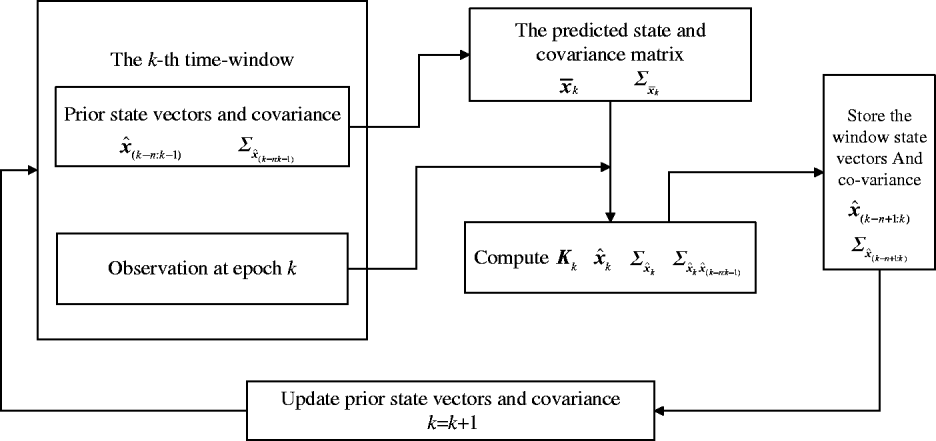
 With the window moving, the new epoch will be introduced and the first epoch of window will be removed. It is rather easy to update the window vector  ${\bi \hat x}_{\left( {k - n + 1:k} \right)} $ and its corresponding covariance matrix ${\bi \Sigma} _{{\bi \hat x}_{\left( {k - n + 1:k} \right)}} $ which is a sub-matrix of Equation (10). One issue should be pointed out that the WRA can reduce to KF when window length n = 1. The WRA implementation from epoch (k − 1) to k is presented in Figure 1.
The computation flowchart of WRA.

3. IMPLEMENTATION OF WRA BASED ON PSEUDORANGE AND DOPPLER MEASUREMENTS
Generally, the GNSS navigation receivers output PV quantities in real time. By utilising the PV solutions generated from GNSS receivers and the Equation (3), the WRA can be directly implemented based on Equations (4) ∼ (12). However, when the number of tracked satellites is less than four, the GNSS receivers’ built-in software cannot generate epoch-wise PV solutions anymore. Nevertheless, the raw GNSS measurements (e.g., pseudorange and Doppler) can still contribute to the PV estimation even if the number of satellites is less than four (Han and Wang Reference Han and Wang2012). Moreover, the raw measurements are more efficient and fundamental in quality control of kinematic system, since raw measurements can be used to identify and correct the errors of either kinematic model or observational model based on robust theory in quality control of navigation system (Yang et al., Reference Yang, Cui and Gao2004).
The GNSS pseudorange observable equation is symbolized at epoch t:
 $$O_r^s \left( t \right) = \left\| {{\bi p}_r \left( t \right) - {\bi p}^s \left( t \right)} \right\| + c\left( {{\rm\Delta} t_r \left( t \right) - {\rm\Delta} t^s \left( t \right)} \right) + {\rm\Delta} Ion_r^s \left( t \right) + {\rm\Delta} Trop_r^s \left( t \right) + {\rm\Delta} Mp_r^s \left( t \right) + \varepsilon _{O_r^s} \left( t \right)$$
where:
- The superscript s denotes the satellite and the subscript r the receiver.
- O is the pseudorange observable.
- ‖pr−ps‖ is the satellite-to-receiver distance from satellite s to receiver r.
- Δt r and Δts are the receiver and satellite clock offsets with respect to the Global Positioning System Time (GPST) in case of GPS system/constellation, respectively.
- c is the speed of light in vacuum.
- ΔIon and ΔTrop reflect signal propagation delays due to the ionosphere and the troposphere, respectively.
- ΔMp is the multi-path effect.
- $\varepsilon_{O_r^s} $ is the un-modelled pseudorange observation error.

Differentiating the pseudorange O rs with respect to time t yields the Doppler observable:
 $$\eqalign{\lambda D_{rk}^s = & \left. {\displaystyle{{dO_r^s \left( t \right)} \over {dt}}} \right|_{t = k} \cr {\rm} = & \displaystyle{d \over {dt}}\left( {\left\| {{\bi p}_r \left( t \right) - {\bi p}^s \left( t \right)} \right\| + c\left( {{\rm\Delta} t_r \left( t \right) - {\rm\Delta} t^s \left( t \right)} \right) + {\rm\Delta} Ion_r^s \left( t \right) + {\rm\Delta} Trop_r^s \left( t \right) + {\rm\Delta} Mp_r^s \left( t \right) + \varepsilon _{O_r^s \left( t \right)}} \right) \right|_{t = k}\cr {\rm} = & \displaystyle{{({\bi p}_{rk} - {\bi p}_k^s})^T \over {\left\| {{\bi p}_{rk} - {\bi p}_k^s} \right\|}}\left( {{\bi v}_{rk} - {\bi v}_k^s} \right) + c\left( {{\rm\Delta} \dot t_{rk} - {\rm\Delta} \dot t_k^s} \right) + {\rm\Delta} I\dot on_{rk}^s + {\rm\Delta} Tr\dot op_{rk}^s + {\rm\Delta} \dot Mp_{rk}^s + \varepsilon _{\dot O_{rk}^s}} $$
where:
- D is the Doppler observable.
- λ is the wavelength of carrier.
- v is the velocity vector.
Pseudorange and Doppler observation Equations (13) and (14) can be written in a matrix form for a single receiver at epoch k as follows:
 $${\bi l}_k = h\left( {{\bi x}_k} \right) + {\bi \varepsilon} _k $$
where:
 $${\bi l}_k = \left[ {\matrix{ {{\bi O}_k} \cr {\lambda {\bi D}_k} \cr}} \right],\quad {\bi O}_k = \left[ {\matrix{ {O_{rk}^{s_1}} & {O_{rk}^{s_2}} & \ldots & {O_{rk}^{s_{m_O}}} \cr}} \right]^T $$
 $${\bi D}_k = \left[ {\matrix{ {D_{rk}^{s_1}} & {D_{rk}^{s_2}} & \ldots & {D_{rk}^{s_{m_{_D}}}} \cr}} \right]^T $$
m O and m D are the number of observed pseudorange and Doppler measurements respectively.
εk is the noise vector of l. ${\bi x}_k = \left[ {\matrix{ {{\bi p}_{rk}} \cr {{\bi v}_{rk}} \cr}} \right]$, prk and vrk are the position and velocity vectors, respectively.
h(·) represents the nonlinear relationships Equations (13) and (14) between pseudorange and xk, and between Doppler and xk, respectively.
Its explicit expression is:
 $$h\left( {{\bi x}_k} \right) = \left[ {\matrix{ {h_O \left( {{\bi x}_k} \right)} \cr {h_D \left( {{\bi x}_k} \right)} \cr}} \right]$$
and:
 $$h_O \left( {{\bi x}_k} \right) = \left[ {\matrix{ {\left\| {{\bi B}_1 {\bi x}_k - {\bi p}_k^{s_1}} \right\| + c\left( {{\rm\Delta} t_{rk} - {\rm\Delta} t_k^{s_1}} \right) + {\rm\Delta} Ion_{rk}^{s_1} + {\rm\Delta} Trop_{rk}^{s_1} + {\rm\Delta} Mp_{rk}^{s_1}} \cr \vdots \cr {\left\| {{\bi B}_1 {\bi x}_k - {\bi p}_k^{s_{m_O}}} \right\| + c\left( {{\rm\Delta} t_{rk} - {\rm\Delta} t_k^{s_{m_O}}} \right) + {\rm\Delta} Ion_{rk}^{s_{m_O}} + {\rm\Delta} Trop_{rk}^{s_{m_O}} + {\rm\Delta} Mp_{rk}^{s_{m_O}}} \cr}} \right]$$
 $$ \eqalign { \tab \hskip -4pt h_D \left( {{\bi x}_k} \right) = \cr \tab \hskip -5pt \left[ {\matrix{ {\displaystyle{{({\bi B}_1 {\bi x}_k - {\bi p}_k^{s_1})^T} \over {\left\| {{\bi B}_1 {\bi x}_k - {\bi p}_k^{s_1}} \right\|}}\left( {{\bi B}_2 {\bi x}_k - {\bi v}_k^{s_1}} \right) + c\left( {{\rm\Delta} \dot t_{rk} - {\rm\Delta} \dot t_k^{s_1}} \right) + {\rm\Delta} I\dot on_{rk}^{s_1} + {\rm\Delta} Tr\dot op_{rk}^{s_1} + {\rm\Delta} \dot Mp_{rk}^{s_1}} \cr \vdots \cr {\displaystyle{{({\bi B}_1 {\bi x}_k - {\bi p}_k^{s_{m_{_D}}})^T} \over {\left\| {{\bi B}_1 {\bi x}_k - {\bi p}_k^{s_{m_{_D}}}} \right\|}}\left( {{\bi B}_2 {\bi x}_k - {\bi v}_k^{s_{m_{_D}}}} \right) + c\left( {{\rm\Delta} \dot t_{rk} - {\rm\Delta} \dot t_k^{s_{m_{_D}}}} \right) + {\rm\Delta} I\dot on_{rk}^{s_{m_{_D}}} + {\rm\Delta} Tr\dot op_{rk}^{s_{m_{_D}}} + {\rm\Delta} \dot Mp_{rk}^{s_{m_{_D}}}} \cr}} \right]$$
with  ${\bi B}_1 = \left[ {\matrix{ {{\bi I}_{3 \times 3}} & {{\bi 0}_{3 \times 3}} \cr}} \right]$ and ${\bi B}_2 = \left[ {\matrix{ {{\bi 0}_{3 \times 3}} & {{\bi I}_{3 \times 3}} \cr}} \right]$, respectively.
It should be pointed out that the systematic errors (such as ionospheric and tropospheric delays) in Equations (13) and (14) can be processed in two ways:
(i) Correct these systematic errors with their empirical models.
(ii) Use the differenced GNSS model to eliminate these errors.
In this paper, (ii) is employed to eliminate the systematic errors. In addition, considering the weak nonlinearity of the GNSS observational model, similar to the EKF, the WRA equations for the GNSS kinematic and observation model can be conducted as follows:
 $${\bi \hat x}_k = {\bi \bar x}_k + {\bi K}_k \left[ {{\bi l}_k - h\left( {{\bi \bar x}_k} \right)} \right]$$
 $${\bi \Sigma} _{{\bi \hat x}_k} = \left( {{\bi I} - {\bi K}_k {\bi H}_k} \right){\bi \Sigma} _{{\bi \bar x}_k} $$
 $${\bi K}_k = {\bi \Sigma} _{{\bi \bar x}_k} {\bi H}_k^T \left( {{\bi H}_k {\bi \Sigma} _{{\bi \bar x}_k} {\bi H}_k^T + {\bi R}_k} \right)^{ - 1} $$
where 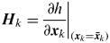 ${\bi H}_k = \left. {\displaystyle{{\partial h} \over {\partial {\bi x}_k}}} \right|_{\left( {{\bi x}_k = {\bi \bar x}_k} \right)} $ is the Jacobian matrix.
Without affecting the accuracy of Equation (14),  $\displaystyle{{{\bi p}_r - {\bi p}^s} \over {\left\| {{\bi p}_r - {\bi p}^s} \right\|}}$ can be replaced by $\displaystyle{{{\bi p}_{rk0} - {\bi p}_k^s} \over {\left\| {{\bi p}_{rk0} - {\bi p}_k^s} \right\|}}$ and prk0 is the approximate position vector of receiver, then Hk is readily derived:
 $$\eqalign{{{\bi H}_k = \left[ {\matrix{ {{\bi H}_{{\bi O}_k}} & {{\bi 0}_{m_P \times 3}} \cr {{\bi 0}_{m_D \times 3}} & {{\bi H}_{{\bi D}_k}} \cr}} \right],\hskip5pt{\rm} {\bi H}_{{\bi O}_k} = \left[ {\openup -3pt\matrix{ {\left( {\displaystyle{{{\bi p}_{rk0} - {\bi p}_k^{s_1}} \over {\left\| {{\bi p}_{rk0} - {\bi p}_k^s} \right\|}}} \right)^T} \cr {\left( {\displaystyle{{{\bi p}_{rk0} - {\bi p}_k^{s_2}} \over {\left\| {{\bi p}_{rk0} - {\bi p}_k^s} \right\|}}} \right)^T} \cr \ldots \cr {\left( {\displaystyle{{{\bi p}_{rk0} - {\bi p}_k^{s_{m_P}}} \over {\left\| {{\bi p}_{rk0} - {\bi p}_k^{s_{m_P}}} \right\|}}} \right)^T} \cr}} \right],}\cr {{\rm} {\bi H}_{{\bi D}_k} = \left[ {\openup -3pt\matrix{ {\left( {\displaystyle{{{\bi p}_{rk0} - {\bi p}_k^{s_1}} \over {\left\| {{\bi p}_{rk0} - {\bi p}_k^s} \right\|}}} \right)^T} \cr {\left( {\displaystyle{{{\bi p}_{rk0} - {\bi p}_k^{s_2}} \over {\left\| {{\bi p}_{rk0} - {\bi p}_k^s} \right\|}}} \right)^T} \cr \ldots \cr {\left( {\displaystyle{{{\bi p}_{rk0} - {\bi p}_k^{s_{m_D}}} \over {\left\| {{\bi p}_{rk0} - {\bi p}_k^{s_{m_D}}} \right\|}}} \right)^T} \cr}} \right]\hskip3pt\cr}$$
where  ${\bi H}_{{\bi O}_k} $ and ${\bi H}_{{\bi D}_k} $ are the coefficient matrices of pseudorange and Doppler measurements respectively.
Because of its first-order linearization, the estimate of WRA is theoretically suboptimal although the second-order term is very small. It is easy to calculate the covariance matrix of  ${\bi \hat x}_k $ and ${\bi \hat x}_{\left( {k - n:k - 1} \right)} $ by:
 $${\bi \Sigma} _{{\bi \hat x}_k {\bi \hat x}_{\left( {k - n:k - 1} \right)}} = \left( {{\bi I} - {\bi K}_k {\bi H}_k} \right){\bi \Phi} _{\left( {k,k - n:k - 1} \right)} {\bi \Sigma} _{{\bi \hat x}_{\left( {k - n:k - 1} \right)}} $$
4. STATE TRANSITION MATRIX MODELLING
Different from the conventional KF model, the WRA use the information of multiple historical epochs rather than just the latest one in the dynamic model. Thus the state transition matrix is relatively complicated. To improve the computation efficiency, two different state transition matrices have been established based on Newton's Forward Difference Extrapolation (NFDE) and Polynomial Fitting (PF) numerical methods in the case when only three-dimensional position is involved in the state vector (Zhou et al., Reference Zhou, Shen and Li2010). Similarly, for the new WRA implementation in this paper, we need of course to construct their corresponding state transition matrices for efficient computations. It is emphasized again that in the new implementation, the state vector is of six-dimensional position and velocity rather than only three-dimensional position.
Here, the establishment of the six-state model will be realized in two steps. First, since the velocity derived from Doppler is commonly more precise than that differentiated by position (e.g., the CV model where the velocity is derived based on the position difference between two consecutive epochs), we employ the velocity estimated by Doppler to predict the current velocity with the NFDE method in a time window. Secondly, we utilize the velocity extrapolation function of time in the window to calculate the position difference between the current epoch and the previous one by Definite Integral (DI) of that velocity function, and then the current position can be reckoned by the position of previous one epoch and the position difference.
4.1. Velocity Derived from the Doppler Based on the NFDE Model
Similar to the extrapolation model in Zhou et al., (Reference Zhou, Li, Rizos and Shen2009, Reference Zhou, Shen and Li2010), the velocity vector v can be assumed as a function of time t, i.e.,vi=v(t i), where vi denotes the velocity vector at epoch t i. By neglecting the high-order remainder terms, the velocity at an arbitrary time can be expressed by the n-th order of NFDE model as:
 $$\eqalign{{\bi v}\left( {t_{k - n + s}, n} \right) = & {\bi v}\left( {t_{k - n} + s\delta t,n} \right) \cr = & {\rm\Delta} ^1 {\bi F}_0 + \displaystyle{s \over {1!}}{\rm\Delta} ^2 {\bi F}_0 + \displaystyle{{s\left( {s - 1} \right)} \over {2!}}{\rm\Delta} ^3 {\bi F}_0 + \ldots + \displaystyle{{s\left( {s - 1} \right) \ldots \left( {s - n + 2} \right)} \over {n!}}{\rm\Delta} ^n {\bi F}_0} $$
where:
- δt denotes the time interval between two consecutive epochs.
- s is the s-th extrapolated epoch s ⩾ n in the time window and n is the order of forward extrapolation. ${\rm\Delta} ^m {\bi F}_0 = \sum\limits_{i = 0}^{m - 1} {\left( { - 1} \right)^{m - 1 - i} C_{m - 1}^i {\bi v}_{k - n + i}} $ with m∈1,\2,\…\n,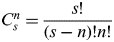 $C_s^n = \displaystyle{{s!} \over {\left( {s - n} \right)!n!}}$ and (·)! is the factorial operator.
Let s=n, then the velocity at epoch k is conducted as (Zhou et al., Reference Zhou, Shen and Li2010):
 $$\eqalign{{\bi v}_k = & {\bi v}\left( {t_{k - n + s}, n} \right) = {\bi Jv}_{\left( {k - n:k - 1} \right)} = \sum\limits_{\,j = 1}^n {J_{n - j + 1}} {\bi v}_{k - j} \cr J_j = & \sum\limits_{i = j - 1}^{n - 1} {\left( { - 1} \right)^{i - j + 1} C_i^{\,j - 1}} C_n^i \quad j \in \left\{ {1,{\rm} 2, \ldots {\rm,} n} \right\}} $$
where:
- ${\bi v}_{\left( {k - n:k - 1} \right)} = \left[ {\matrix{ {{\bi v}_{\left( {k - n} \right)}^T} & {{\bi v}_{\left( {k - n + 1} \right)}^T} & \ldots & {{\bi v}_{\left( {k - 1} \right)}^T} \cr}} \right]^T $ represents a 3n column vector of velocities for all n epochs in the window.
- ${\bi J} = \left[ {\matrix{ {J_1} & {J_2} & \ldots & {J_n} \cr}} \right] \otimes {\bi I}_{3 \times 3} $ is a 3 × 3n constant coefficient matrix with ⊗ being the Kronecker product.


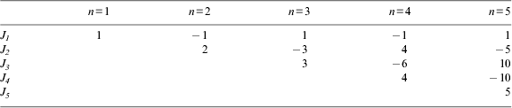
In real applications, the coefficient matrix J is primarily computed offline and its elements for 1≤n ≤ 5 are presented in Table 1.
The coefficient matrix J for the different window lengths (n = 1 to 5)

4.2 Position Derived from Velocity Based on the DI Method
As is well-known in mathematics, in general the differential algorithm augments error while the integral reduces error. Thereby, the definite integral of velocity is introduced to diminish the position errors. At epoch k, position vector can be expressed by position of epoch k − 1 and the position difference from epoch k − 1 and k:
 $${\bi p}_k = {\bi p}_{k - 1} + {\rm\Delta} {\bi p}_{k,k - 1} $$
where Δpk ,k−1 is the position difference vector from epoch k − 1 to k.
It is rather easy to obtain the position difference of two consecutive epochs which can be recovered by the definite integral of velocity from previous one epoch to current epoch:
 $${\rm\Delta} {\bi p}_{k,k - 1} = \int_{t_{\left( {k - 1} \right)}} ^{t_k} {{\bi v}\left( {t_{k - n + s}, n} \right)} dt_s = \int_{k - 1}^k {{\bi v}\left( {t_{k - n + s}, n} \right)} ds$$
Inserting Equation (21) into Equation (24), we obtain the linear combination of velocity vectors in the time window:
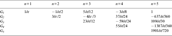
 $${\rm\Delta} {\bi p}_{k,k - 1} = {\bi Gv}_{\left( {k - n:k - 1} \right)} = \sum\limits_{i = 1}^n {G_{n - i + 1}} {\bi v}_{k - i} $$
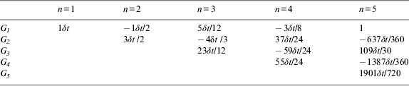
Similar to J, the coefficient matrix G is also computed offline and its elements for 1≤n ≤ 5 are presented in Table 2.
The coefficient matrix G for the different window lengths (n = 1 to 5)
Finally, the following dynamic model is established based on Equations (22) and (23):
 $$\left[ {\matrix{ {{\bi p}_k} \cr {{\bi v}_k} \cr}} \right] = \left[ {\matrix{ {{\bi p}_{k - 1} + {\bi Gv}_{\left( {k - n:k - 1} \right)}} \cr {{\bi Jv}_{\left( {k - n:k - 1} \right)}} \cr}} \right] + \left[ {\matrix{ {{\bi w}_{k1}} \cr {{\bi w}_{k2}} \cr}} \right]$$
 Let  ${\bi x}_k = \left[ {\matrix{ {{\bi p}_k} \cr {{\bi v}_k} \cr}} \right]$, ${\bi x}_{\left( {k - n:k - 1} \right)} = \left[ {\matrix{ {{\bi x}_{k - n}^T} & {{\bi x}_{k - n + 1}^T} & \ldots & {{\bi x}_{k - 1}^T} \cr}} \right]^T $ and ${\bi w}_k = \left[ {\matrix{ {{\bi w}_{k1}} \cr {{\bi w}_{k2}} \cr}} \right]$, then Equation (26) is reformulated as:
 $${\bi x}_k = {\bi \Phi} _{k,\left( {k - n:k - 1} \right)} {\bi x}_{\left( {k - n:k - 1} \right)} + {\bi w}_k $$
where Φk,(k − n:k − 1) denotes the state transition matrix that is dependent on the time window length n and the time interval δt.
Once the window-length n and δt are given, Φk,(k − n:k − 1) will be a constant matrix defined as:
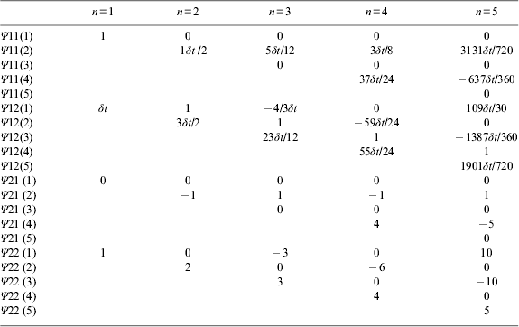
 $${\bi \Phi} _{k,\left( {k - n:k - 1} \right)} = \left[ {\matrix{ {{\bi \Phi} _{11}} & {{\bi \Phi} _{12}} \cr {{\bi \Phi} _{21}} & {{\bi \Phi} _{22}} \cr}} \right] = \left[ {\matrix{ {{\bi \psi} _{11}} & {{\bi \psi} _{12}} \cr {{\bi \psi} _{21}} & {{\bi \psi} _{22}} \cr}} \right] \otimes {\bi I}_{3 \times 3} $$
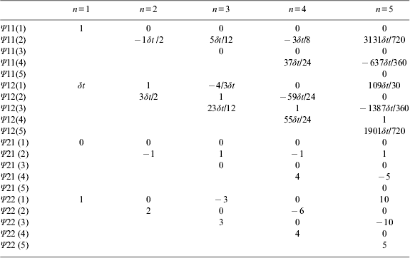
where ψ11, ψ12, ψ21 and ψ22 are all (n×n) coefficient matrices.
Their elements for the window length n from 1 to 5 are shown in Table 3.
The coefficient matrix Ψ for the different window lengths (n = 1 to 5)
5. EXPERIMENT AND ANALYSIS
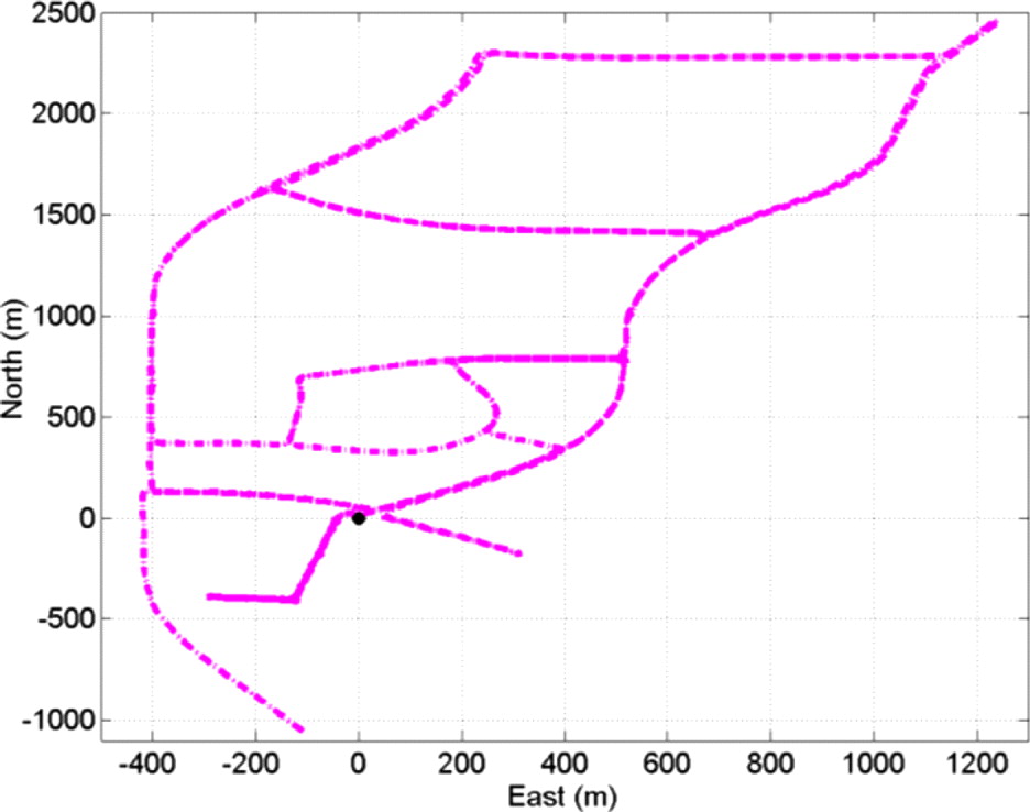
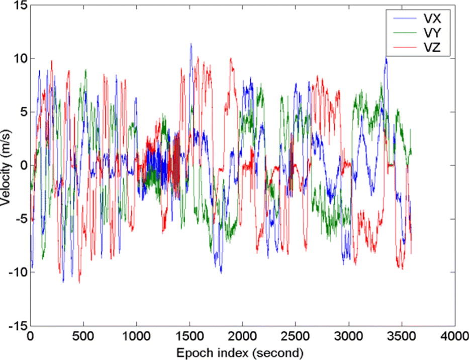
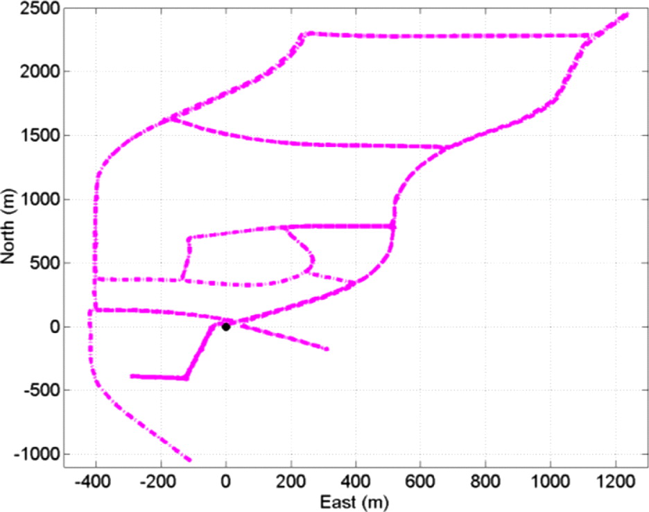
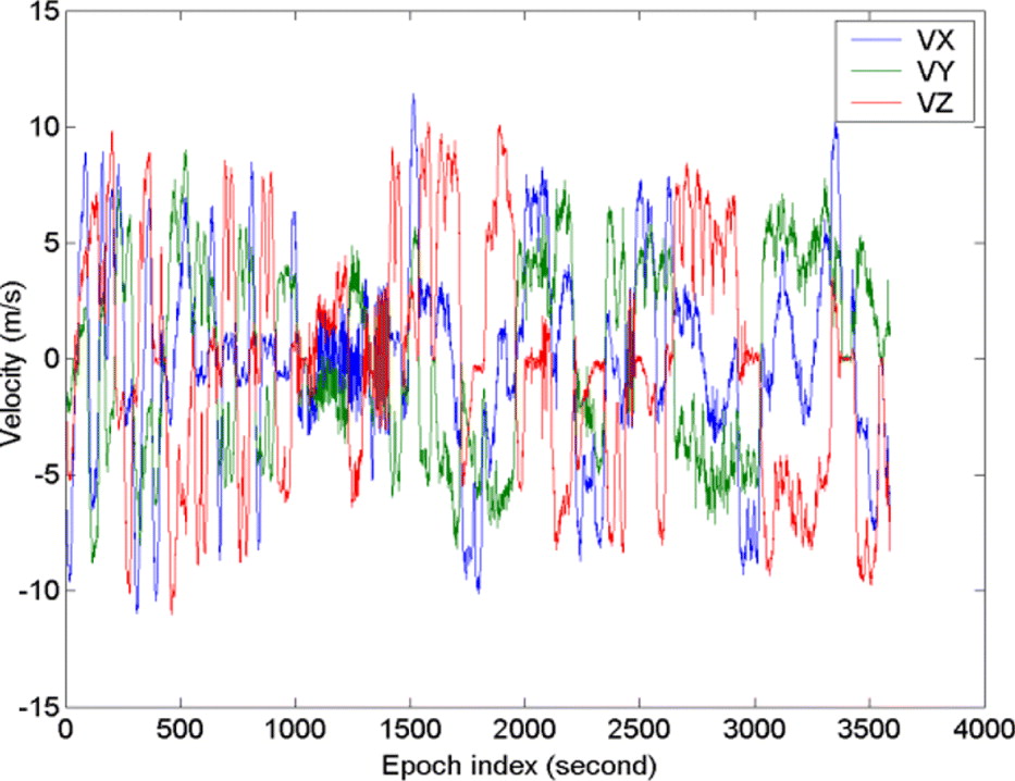
The experiment data were collected by using two Topcon HiPer-Pro GPS receivers with a sampling interval of 1 second. Although the maximal distance between the reference and rover stations is shorter than 3 km (see Figure 2), the various kinematic states are intentionally experienced in the whole vehicular GPS test. The estimated three-dimensional velocities of the vehicle by using the Doppler measurements are shown in Figure 3. The double differenced observation model is used in the experiment and the systematic errors are basically ignored due to their highly spatial correlation in such a short distance between reference and rover stations. The C/A code and Doppler D1 measurements were utilized in the whole test. The results computed by use of the dual-frequency carrier phase measurements (resolved by Ashtech solution GPS software 2.6) are used as the reference values to evaluate the accuracies of the developed models.
The horizontal (East – North) trajectory of vehicle.
Velocities of X, Y and Z components.
In the following section, we will investigate the accuracies of our WRA in the cases of the different window lengths and the different sampling intervals. In our computation strategy, the weight matrix of double differenced GPS observations was derived from the C/N0 weighted matrix of undifferenced observations by using the law of error propagation (Kuusniemi et al., Reference Kuusniemi, Lachapelle and Takala2004). The researches have indicated that the stochastic model of wk is also an important issue to affect the solution. Therefore, to obtain the optimal solution, the reasonable stochastic model should be determined in real-time (Wang Reference Wang2000; Moore and Wang Reference Moore and Wang2003, Hewitson and Wang Reference Hewitson and Wang2007; Geng and Wang Reference Geng and Wang2008; Yang and Gao Reference Yang and Gao2005). In this paper, without affecting the validity and efficiency of our WRA, for simplification, the covariance matrix Σ w was selected as a (6 × 6) matrix with spectral density of 0·2m2s−3 as follows (Schwarz et al., Reference Schwarz, Cannon and Wong1989):
 $${\bi \Sigma} _{{\bi w}_k} = \left[ {\matrix{ {\displaystyle{1 \over 3}\delta t^3} & {\displaystyle{1 \over 2}\delta t^2} \cr {\displaystyle{1 \over 2}\delta t^2} & {\delta t} \cr}} \right] \otimes {\bi Q}$$
where:
- Q is a 3 × 3 diagonal matrix with the elements of spectral density for velocities.
- δt denotes the sampling time interval.
The initial position and velocity variances were cautiously chosen as 1 m2 and 0·1 m2/s2 respectively. The transition matrix of the dynamic model established in Section 4 was used.
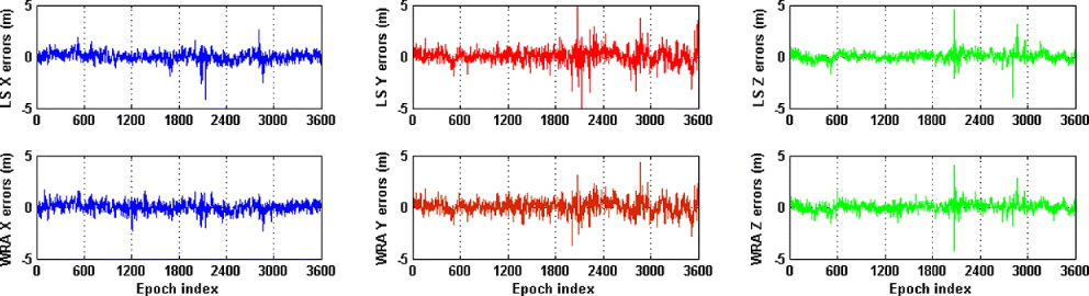
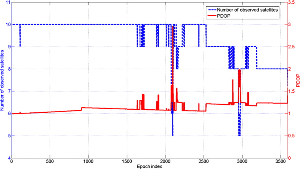
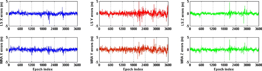
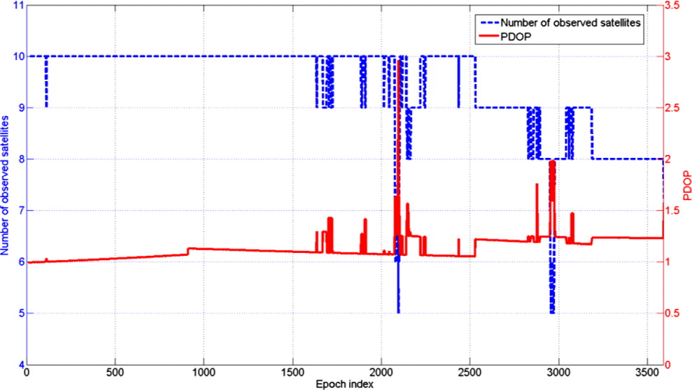
For the sampling rate of 1 s that is referred to as the high sampling rate, the differences of Least Squares (LS) solutions and WRA (n = 1) with/without Doppler measurements from reference values are shown in Figure 4. The accuracy statistics of LS and WRA (n = 1) solutions are presented in Table 4. It is easy to theoretically prove that the solution of WRA with n = 1 is exactly equivalent to the KF solution with CV dynamic model. Hence, herein they are not particularly compared with each other. Figure 5 shows the number of observed satellites (blue dashed line) and the Position Dilution Of Precision (PDOP) (red solid line). It can be seen from the Table 4 and Figure 4∼5 that:
(i) the poor solutions are generally assigned to the larger PDOP values, especially during the observation epochs from 2000 and 3000, which is mainly caused by the rapidly decreasing of observed satellites.
(ii) LS outperforms WRA (n = 1) without Doppler, because the kinematic model of WRA (n = 1) cannot accurately describe the moving object's manoeuvring motions, for instance, turning, accelerating and braking.
(iii) Aided by the kinematic model of the vehicle, compared with LS, WRA can improve the positioning accuracies in the case of the number of observed satellites sharply decreasing.
(iv) Since the Doppler measurements provide the accurate velocity quantities, WRA with Doppler is obviously better than that without Doppler, especially in poor observation conditions.
Differences of LS and WRA (n = 1) solutions from the reference values for sampling interval of 1 s (top: Differences of LS from the reference values; bottom: Differences of WRA without Doppler implementation).
The number of observed satellites and PDOP during kinematic GNSS navigation.
RMSE (m) of WRA with and without Doppler implementations (n = 1) (1 s)

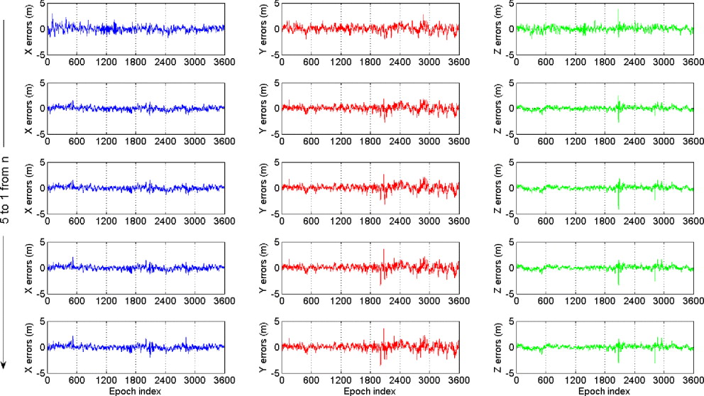
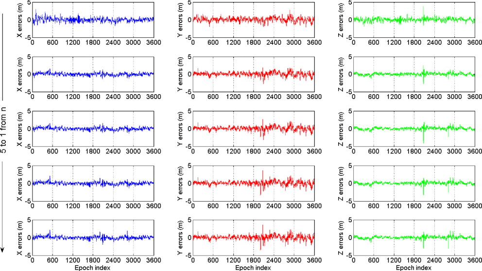
We also calculated the differences of the Doppler-aided WRA solutions based on the six-state model from reference values, which are illustrated in Figure 6. Moreover, the efficiency of constructed dynamic models of WRA is examined in the window length n from 1 to 5. The Root-Mean-Squared Error (RMSE) of three position components and position are computed by Equations (30) and (31) respectively:
 $${\rm RMS}\left( X \right) = \sqrt {\displaystyle{{\sum\nolimits_{i = 1}^q {{\rm\Delta} X_i^2}} \over q}} \quad {\rm RMS}\left( Y \right) = \sqrt {\displaystyle{{\sum\nolimits_{i = 1}^q {{\rm\Delta} Y_i^2}} \over q}} \quad {\rm RMS}\left( Z \right) = \sqrt {\displaystyle{{\sum\nolimits_{i = 1}^q {{\rm\Delta} Z_i^2}} \over q}} $$
 $${\rm RMS}\left( {POS} \right) = \sqrt {{\rm RMS}\left( X \right)^2 + {\rm RMS}\left( Y \right)^2 + {\rm RMS}\left( Z \right)^2} $$
where:
- ΔX, ΔY and ΔZ represent the three position difference components between our WRA solutions and the referenced ones.
- RMS(·) denotes the RMSE of position and the symbol POS denotes the point position.
- Here q is the number of all observed epochs.
The computed RMSE statistics are shown in Table 5. Based on experimental results so far in Table 5 and Figure 6, it is concluded that:
(i) In the case of n = 2, the WRA solution is obviously superior to the solution of n = 1.
(ii) With the window length n increasing (n > 2), the accuracies decrease but the extent is not so obvious.
(iii) For those vehicles with high sampling rate (δt < 1 s) or manoeuvrability, the window length should not exceed 5 epochs. It is worth pointing out that the dynamic model in WRA of n = 2 actually works as the CA model and is also compatible with the CV model.
The differences of the WRA solutions from the reference values for sampling interval of 1 s.
RMSE (m) of WRA with different window lengths (n = 1 to 5) in GPS navigation (1 s)

However, those dynamic models with larger windows (n > 2) do not achieve the expected solutions for two reasons:
(i) the dynamic characteristics are over modelled when n > 2.
(ii) The errors of NFDE and DI combined dynamic model sharply augmented with the window length n increasing, therefore the window length should be carefully chosen according to different application scenarios.
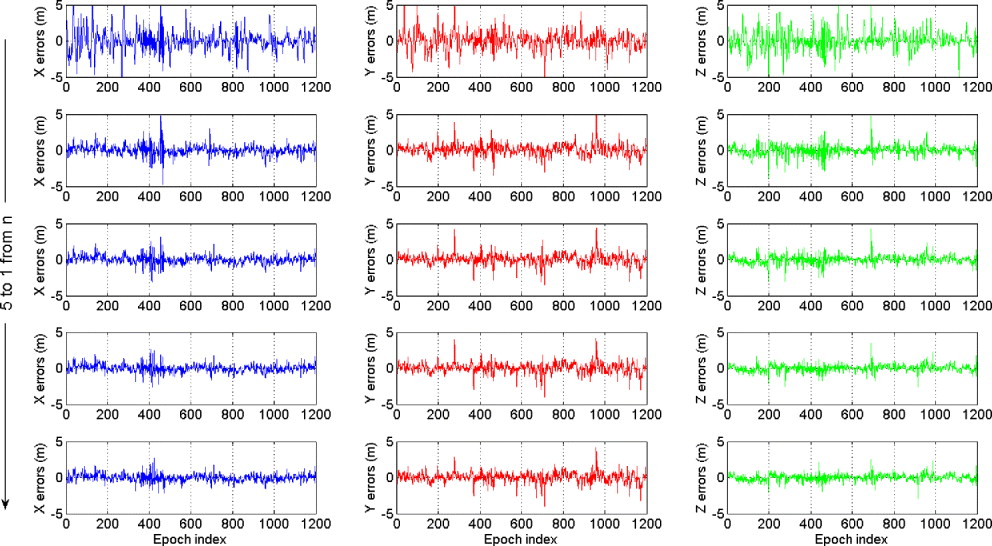
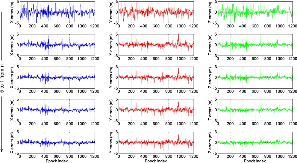
We further tested the performances of the Doppler-aided WRA in the lower sampling rate. The data is thinned in the sampling interval of 3 s and the computation strategy is the same as in the former experiment. The differences between the WRA solutions and the reference values are illustrated in Figure 7. The RMSE statistics computed in terms of Equations (30) and (31) are shown in Table 6. It is observed that:
(i) The RMSE statistics of WRA with different window lengths in Table 6 are generally greater than those in Table 5.
(ii) Some simple assumptions on the dynamic model of moving objects e.g. vehicle, CV (n = 1) and CA (n = 2), are not appropriate any more.
(iii) As the window length n increases, our WRA performs better and its accuracy is improved.
(iv) Compared with CV and CA dynamic models, those higher-order dynamic models (n > 2) accurately describe the characteristics of vehicle's motion and thus improve the navigation solutions in lower sampling rate scenario.
The differences of the WRA solutions from the reference values for sampling interval of 3 s.
RMSE (m) of WRA with different window lengths (n = 1 to 5) in GPS navigation (3 s)

6. CONCLUSIONS
In summary, the implementation of Window-Recursive Approach (WRA) based on pseudorange and Doppler measurements has been developed for GNSS navigation. A state transition matrix was constructed based on the Newton's Forward Difference Extrapolation (NFDE) and Definite Integral (DI) methods for efficient computation. Real vehicular GPS experiments were carried out to evaluate the specified implementation of WRA in two sampling data scenarios. The results show that:
(i) in the high sampling rate, the low-order models can describe the motion states adequately and achieve the optimal results in the window length less than 5 epochs. Conversely, in the low sampling rate, the low order models cannot specify the motion states well enough. Therefore, high-order models with longer window length are necessary to achieve better performances.
(ii) WRA is flexible and efficient in Global Navigation Satellite Systems (GNSS) navigation computation. It reduces to a Kalman filter if window length n is set to 1.
(iii) The varying velocity and acceleration of a vehicle's motions can be automatically specified in the high-order models of WRA, therefore it does not need to construct the velocity and acceleration dynamic models for predicting the Position and Velocity (PV) state epoch by epoch.
In the future, we will further investigate the issues of WRA potential implementation fields, including optimal window length determination, nonlinear transformation problem and quality control framework etc. In addition, our WRA for GNSS kinematic navigation provides highly precise position and velocity information, which can also be implemented to accurately estimate Inertial Navigation System (INS) errors in GNSS/INS navigation or to detect faults in integrated navigation systems as a trajectory constraint condition.
ACKNOWLEDGEMENTS
The work is supported by the Fundamental Research Funds for the Central Universities (Grant No. ZYGX2010J114) and Natural Science Foundations of China (Grant No. 41074018), and partially supported by Kwang-Hua Fund for College of Civil Engineering, Tongji University and the fund from the State Key Laboratory of Information Engineering in Surveying, Mapping and Remote Sensing, Wuhan University (Grant No. 10P01).