1. Introduction

According to Reference Armstrong, Armstrong, Roberts and SwithinbankArmstrong and others (1966), the kinds of ice which first form in wind-agitated seas are called frazil and grease ice. They define frazil ice (p. 16) as “fine spicules or plates of ice in suspension in water” and grease ice (p. 18) as “a later stage of freezing than frazil ice, where the spicules and plates of ice have coagulated to form a thick soupy layer on the surface of the water”.

More recent research in both rivers and oceans summarized by Reference MartinMartin (1981) shows that the basic crystal which makes up the frazil-ice suspension is a disc measuring about 1–3 mm in diameter and 1–10 μm in thickness. In the present paper we refer to suspensions of these individual discs as “frazil ice”. Second, both from the present experiments and those of Martin and others (1979, hereafter abbreviated MKW), we find that grease ice is a dense slurry of the individual frazil platelets with concentrations by volume in sea-water of 20–40% ice. Within the grease ice the individual crystals rapidly sinter together to form larger irregular ice clumps.

The present paper focuses on the wave-absorption properties of grease ice. Section 2 describes a variety of field observations on how grease ice forms in the Chukchi and Bering Seas. Then Section 3 describes our laboratory apparatus and technique, and Section 4 gives a general qualitative discussion of the grease ice. Next, Section 5 reviews the applicable water-wave theory, and Section 6 discusses the quantitative results of our wave-decay and iceconcentration measurements. Finally, Section 7 shows that, if a yield-stress model describes the grease-ice viscosity where the yield stress coefficient increases with the wave momentum flux, then the model describes the observed wave decay.

2. Field observations

In large polynyas, grease ice forms in long rows parallel to the wind. Reference Dunbar and WeeksDunbar and Weeks (1975) describe such rows forming in the Gulf of St Lawrence, and Moira Dunbar (private communication in 1976) suggests that these rows are the result of a Langmuir circulation. To illustrate, Figure 1 shows an oblique view from a helicopter of grease-ice formation in a large polynya about 2 km wide and many kilometers long off Nome, Alaska, on 5 March 1978. The helicopter altitude is about 150 m; the floe diameter in the center of the photograph is about 100 m. The air temperature was —20°C, and the wind speed was 15 m s⁻¹ from 010°. The photograph shows the long plumes of grease ice which form approximately parallel to the wind. It also shows that the grease ice piles up down-wind against the floes, where the incident waves damp out within four to six wavelengths. Films made of this wave damping show that the dominant wave period is 1.8–2.2 s, so that the wavelength in the photograph is about 6 m. Finally, the arrow in Figure 1 marks what appears to be a detritus line, which we discuss in Section 4.

Fig.1. Oblique aerial photograph from 150 m of grease-ice formation in a large polynya south of Nome, 5 March 1978. See text for further discussion.

Although we were unable to sample the grease-ice thickness at this site, four days later after the winds had died down and the grease-ice surface had congealed, we measured the thickness on the windward side of another polynya. In this measurement, we cut holes through the newly-frozen grease ice, then slowly lowered a transparent tube 1 m long with 40 mm inner diameter into the grease ice, rotating the tube as we lowered it. After the tube was almost submerged, we put a rubber cap firmly over the top, slowly raised it out of the water, then measured the grease-ice thickness through the side. From three measurements along a 10 m distance, we found grease-ice thicknesses of 0.7 m, 1 m, and > 1 m. As Sections 5 and 6 show, for 2 s waves the grease-ice thickness or k⁻¹-depth at which rapid wave decay begins is 1 m. This observation suggests that the thickness of the piled-up grease ice in Figure 1, which grew under similar meteorological conditions, may also have been at least 1 m.

For another example, Figure 2 is an aerial photograph taken at a radar altimeter height of 147 m from the NASA Convair-990 on 20 February 1973 over the Bering Sea (private communication from P. Gloersen), The flight heading was 185°, at altitude the air temperature was —14°C, and the wind speed and direction were 11.5 m s⁻¹ from 332°, so that the plumes again line up parallel to the wind. From inspection of the photograph, the predominant ocean wavelength is about 1.5 m. The photograph also shows that the grease-tee plumes range in width from less than 1 m to 35 m across for the plume at the lower left, and that the cross-wind distance between the plumes ranges from 2–4 m for the small plumes to about 170 m for the very wide plumes. From the photograph the characteristic shape of several of the plumes consists of an up-wind tail and a broad head, referred to by Reference Dunbar and WeeksDunbar and Weeks (1975) as “tadpoles”. The arrows at the top and sides of the photograph mark examples of (Figure 2) these tadpoles, where the heavy arrow to the left marks the best example. For these plumes there is an obvious pile-up of grease ice in the head, and visible on the original negative at least, a wave shadow or absence of waves behind the heads.

Fig.2. Aerial photograph from 147 m of grease-ice formation in a large polynya ; photograph measures 205 m across, and north is to the top. See text for discussion of arrows (photograph courtesy of NASA).

These plumes also appear to be visible on satellite photographs. Figure 3 shows a Landsat image of the polynya south of St Lawrence Island in the Bering Sea for 17 March 1976. The weather charts both for this day and the preceding three days show that a strong high-pressure system over Siberia created north-easterly winds over the Bering Sea. On 17 March at 18.00 Z, or approximately 1 h before the Landsat image was taken, the station “Wales” on Cape Prince of Wales north of St Lawrence Island reported an air temperature of —25°C and north-easterly winds of 15 in m s^–1. The image shows that these cold winds caused the growth of many small streaks in the dark water south of St Lawrence Island, which form together into larger streaks, and finally pile up down-wind into clumps perpendicular to the wind. The scales of the large plumes shown in Figure 2, namely widths of about 35 m separated by 170 m accompanied by the high contrast between the ice and water and the long linear nature of the streaks, suggest that they are resolvable by the 70 × 70 m² Landsat pixel size. From other Landsat images on the same day we observed similar features south of both Cape Prince of Wales and Diomede Islands; we have also observed (Figure 3) these parallel streaks on Landsat images from March 1979. These Landsat observations strongly suggest that regions of grease-ice formation can be mapped by satellite.

Fig.3. Landsat image of grease-ice formation in the polynya south of St Lawrence Island; the image width is 185 km; the pixel size is 70 m × 70 m.

Physically, the Langmuir circulation consists of oceanic roll vortices which herd the frazil crystals into plumes. Figure 4, adapted from Pollard (1977, fig. 8.3) schematically shows the vortices with their alternating directions of rotation and the resultant surface convergence zones where the grease ice accumulates. In a theoretical discussion, Reference Craik and LeibovichCraik and Leibovich (1976) show that the interaction of the bi-directional wind-wave spectra with the surface wind drift generates this circulation. They also suggest that the presence of contaminants causing wave attenuation such as grease ice in the convergence zones intensify the Langmuir circulation and thus the ice accumulation rate in the zones. The presence of grease ice in the plumes, then, may itself lead to greater accumulations. Finally, both theory and observations show that the down-wind surface drift in the convergence zones transports the ice out of the upwind region of the polynya and thus clears the water surface for new ice growth.

Fig.4. Schematic diagram of the Langmuir circulation (adapted from Reference Pollard and KrausePollard, 1977).

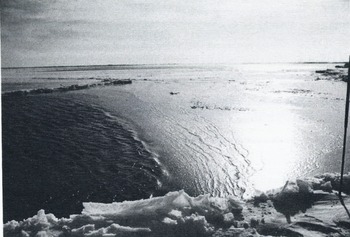
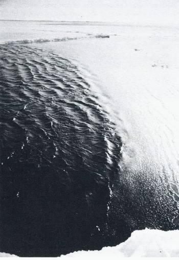
In small Arctic leads the grease ice is not herded into Langmuir plumes; rather, as we have observed in many small leads in the Beaufort, Chukchi, and Bering Seas, cold winds cause both the growth of small wind waves and the formation and herding of grease ice to the down-wind end of the lead. Figures 5 and 6 show such a lead near Cape Lisburne on 16 March 1978 at an air temperature of —16°C and a wind speed of 10 m s⁻¹. The lead had a wedge shape, about 15 m wide in the cross-wind direction at the boundary between the grease ice and the seawater, and about 50 m long with the apex of the wedge up-wind. Figure 6 shows that the waves which had lengths of 100 mm, abruptly damp out as they enter the grease ice. Also measurements of the grease-ice thickness using the tube technique described earlier showed that the thickness at a distance of 0.1 m in from the leading edge was 80 mm, and in the region behind the wave damping was 50 mm. The photographs also show small pancakes forming on the grease ice similar to those reported in MKW.

Fig.5. Grease-ice formation in a small lead.

Fig.6. Close-up of the grease ice edge in Figure 5.

For the same lead we observed ice crystals in water samples from the open water up-wind of the grease ice. We took these samples with a plastic beaker which we first rinsed in sea-water so that the beaker and water temperature equilibrated. We then scooped out a sea-water sample at a distance of about 20 m up-wind of the grease ice and held it quickly up to the sun; in the sea-water we immediately saw interior reflections from very small crystals. This observation supports our speculation that the crystals form in the open water, and then are herded down-wind into the grease ice. The ice in this lead then grew both vertically from heat loss through the solid ice, and laterally from advected crystals.

3. The experiment

The experiment took place in an insulated tank with inner dimensions of 2 m in length, 1 m in width, and 0.6 m in depth, shown in Figure 7. The tank consisted of an inner tank made from 13 mm thick “Plexiglas” (polymethyl methacrylate) which rested in an outer tank made of 50 mm thick polyurethane foam which was held together and supported 0.3 m above the floor by a wooden frame. At the bottom of the inner tank a stainless-steel sheet served as a ground for the wave probes. The tank was located in a large cold room where the temperature could be varied from +5°C to –35°C with an accuracy of ±1 deg. To observe the waves, we cut removable windows which extended over the tank length into the foam of one side wall. To minimize the heat flux through the tank bottom, we surrounded the air space under the tank with an insulating curtain, then placed two 100 W light bulbs in this air space. During the experiment a proportional temperature controller turned these bulbs on and off to maintain the air temperature at the water temperature of –2°C.

Fig.7. A schematic, side-view drawing of the apparatus.

A paddle mounted at one end of the tank generated the waves; the paddle consisted of a 60° wedge measuring approximately 0.43 m high, 0.24 m wide, and 0.96 m long, so that it nearly spanned the tank. In the middle of the upper wedge surface we mounted a single vertical rectangular steel shaft 0.8 m long, which was supported by two square linear bearings attached to the tank, and terminated in a Scotch Yoke. To drive the paddle in oscillatory vertical motion, an adjustable eccentric mounted on the drive shaft of a stepping motor drove the Scotch Yoke with a maximum peak-to-peak amplitude of about 100 mm. A power amplifier coupled to a frequency generator drove the stepping motor at 200 steps per revolution; we typically operated the motor at frequencies between 340 and 500 Hz with an accuracy of 1 Hz.

For an experiment we filled the tank to a depth of 0.41 m with a 35.5‰ NaCl solution, which has a freezing point of –2.15°C. By setting the room temperature to –2°C, we cooled the tank to a temperature between o and —2°C. To grow ice, we then lowered the room temperature to —25°C, blew air over the tank with two small fans, and turned on the paddle at a low amplitude and frequency to prevent the resonant build-up of large wave amplitudes. Because the inside tank walls cooled faster than the water, ice first formed on the tank walls from splashing. Then, as the water temperature approached —2.1°C, small frazil crystals formed on the water surface and were advected down-wind. Finally, when the water temperature reached —2.1°C, small disc-like crystals filled the tank interior in an upside-down snow-storm throughout the entire depth. After formation, the crystals rose slowly to the surface with their c-axes parallel to gravity until they reached the depth of the wave oscillations, above which the crystals moved with the waves. On reaching the surface, the wind and waves advected the crystals to the far end of the tank, where they collected in a small wedge similar to that shown in Figures 7 and 9.

Fig.9. Comparison of a composite side-view photograph of the grease ice in the tank with a drawing of the mean circulation in the grease ice. A tank support causes the gap in the composite photograph. See text for further discussion.

As the amount of ice within this wedge increased, the wave damping became more efficient. Therefore, we increased both the paddle amplitude and frequency to crowd the grease ice into as short and as deep a wedge as possible consistent with no splashing of water out of the tank. In this way we grew a grease-ice layer of average thickness 0.15 m in less than 1 h. When the amount of ice in the tank reached half its desired value, we raised the room temperature to —3°C, then let the heat transfer from the water to the room both to warm up the room and to grow more ice.

To measure wave amplitudes in the grease ice, we used conductivity probes consisting of stainless-steel, 24 gauge hypodermic needles 100 mm long. To avoid icing of these probes, we ran our wave damping experiments at air temperatures only slightly below the sea-water freezing point. The justification for running at these warm temperatures came from the observations discussed in MKW and below in Section 4; namely that even for air temperatures as low as —30°C the grease-ice surface temperature over most of the decay region was only 0.1–0.01 deg colder than the sea-water freezing temperature. Therefore we assumed that running our wave damping experiments at a warm temperature did not alter the properties of the grease ice.

Figure 8 is a schematic diagram of the probe configuration and the accompanying circuitry. The needle was mounted on the end of a 30 mm diameter “Plexiglas” tube; inside this tube, an a.c. bridge, which was driven by the oscillator power supply at 300–600 Hz, and a precision a.c.-to-d.c. converter converted the wave amplitude to a d.c. voltage. Outside the cold room the d.c. output was connected either to a digital voltmeter and an x–y plotter for calibration of the probe, or to a Brush eight-channel amplifier and pen recorder for the wave experiments. Calibration of the probes showed that they were linear to within ±0.5 mm except when the probe was either nearly completely submerged or nearly out of the water. Physically, the probes behaved well in the wave field. For large-amplitude waves the probes bent with the waves on the order of 5–10°, but because the amplitude measured with the probe varied with the cosine of the bending angle, this had only a small effect. Also, the crystals generally appeared to wash smoothly around the needle with only an occasional ice crystal leaning up against it.

Fig.8. The probe circuitry: A, the conduclivity bridge; B, precision a.c.-to-d.c. converter; C, oscillator and power supply; D, eight-channel amplifier; E, eight-channel Brush recorder; F, digital voltmeter; G, x–y plotter.

To measure the decay of waves with distance, we mounted approximately over the center of the tank a wooden beam which ran the length of the tank with notches cut into it at 50 mm intervals as probe supports. During an experiment we first placed the probe in the open water just ahead of the ice, and left it at that position for about 50 wave periods. A strip chart recorded the probe output; during the experiments one of us positioned the probe, the other logged the probe position on the chart paper. We would then move the probe down the tank in 50 or 100 mm increments with a pause of 20—50 wave periods at each station. The shorter recording periods were used only for the low wave amplitudes. We continued this process until the wave amplitude was less than 0.5 mm.

The probe traverse took between 20 and 30 min. After completion of the traverse, we next measured the grease-ice thickness at different distances from the paddle while we continued to generate waves. We measured this thickness in the wave trough at 0.1 m intervals down the tank by holding a ruler against the side of the “Plexiglas” window, then recording the minimum height of both the top and bottom of the grease ice. This measurement is the minimum thickness; the maximum occurs at the wave crest. For large amplitudes, where the ice thickness is either less than or on the order of the wave amplitude, this measurement is accurate to only 10–20 mm. As the wave amplitude decreased and the ice thickness increased with distance down the tank, this measurement became both more accurate and more representative.

We also recorded the ice thickness photographically. To do this, we used a 800 W s flash bulb and reflector unit which was mounted about 1.2 m above the tank on a movable carriage. For each experiment we then look flash photographs of the ice through the windows at three pre-set positions; these photographs were later assembled into the composites shown in Figures 9 and 13.

Fig. 13 Side-view photographs of four wave-damping experiments at σ = 14.9 s⁻¹, corresponding to the 24 May experiments in Table 1. A tank support causes the gap in each composite photograph; above each composite, the position of the open arrows mark the depth k⁻¹; the dark arrows mark the dead zone. Paddle amplitude ranges from (a) 10 mm, (b) 11.5 mm, (c) 13 mm, (d) 14.5 mm.

Finally, in several of the experiments we determined the relative ice volume of the grease ice as a function of distance. In our technique we set up a series of ten 250 ml graduated cylinders on a bench in our cold room. In the top of each cylinder we placed a funnel with a stem of inner diameter 6 mm. Then we set the room temperature at —3°C and, using a 250 ml beaker, we scooped ice-water samples from the tank at the wave crests in scoops parallel to the crests at 0.1 m intervals down the tank. We quickly poured the sample into the funnel, where the constriction retained the ice while the brine flowed through. After the brine had drained from the ice, we measured the volume of brine, then mixed the ice and brine together and poured them into a jar which was subsequently sealed. This sample was allowed to melt, after which we measured the total sample volume and salinity. As Section 6.3 shows, these measurements, along with the open-water salinity, allow us to determine both the ice concentration and salinity.

4. General properties of grease ice

This section discusses first the large-scale behavior of grease ice, then the small-scale properties of ice crystals. For the first, Figure 9 compares a side-wall composite photograph of the grease ice with a schematic drawing of the observed circulation. In the composite photograph the paddle is to the left, the grease ice is white and increasing in thickness to the right, and the wave probe is visible at the upper left.

Below the photograph the schematic diagram shows several features of the ice circulation. First, in the open water to the left, the figure shows the individual ice crystals rising to the surface. Once these crystals reach the surface, they are swept into the grease ice by the Stokes drift. Second, both the photograph and the schematic drawing show that the grease ice is herded to the right into a long oscillatory wedge. Section 5.2 shows that the cause of this grease-ice wedge is the balance between the decrease of the wave-momentum flux and the free-surface tilt. Third, the diagram shows a vertical line marked as the “dead zone”, which divides the grease ice into regions of “liquid” and “solid” behavior respectively to the left and right. Finally, the arrows within the liquid grease ice show the direction and approximate magnitude of the mean circulation, where we omit the wave orbital velocities.

From our experiments we found that the dead zone is a vertical transition zone 5–10 mm wide, in the grease ice between regions of fluid and solid behavior. To the left of the dead zone the waves propagate as water waves with strong relative motions within the ice, and the ice thickness depends only on distance from the leading edge. To the right the ice appeared to move as an elastic solid with no internal relative motion and as the photographs in Figure 13 partially show, the lower surface consisted of three-dimensional billows. In short, when we deformed the ice to the right, it stayed deformed, whereas for the ice to the left, deformations disappeared within one to five wave periods. These observations suggest that at low or non-existent shear rates the grease ice behaves as a solid, while at high shear rates it flows as a liquid.

For a surface view of the dead zone, Figure 10 shows a side-view photograph of the grease ice at a frequency of 10.7 s⁻¹ and wave amplitude of 28.5 mm, where the probe support runs along the bottom. To the left is the boundary between open water and the grease ice; to the right the line of bubbles marks the dead zone. Breaking waves at the leading edge generate these bubbles, which the mean circulation carries to the dead zone. In general, the dead zone serves both as a transition between liquid and solid behavior and as an accumulation line for material released on the surface. Possible field examples of the dead zone include an obvious case of the detritus line marked by the arrow in Figure 1, and the thick ice build-up around the heads of the arrow-marked Langmuir plumes in Figure 2. Because the ice in these heads is thicker than the up-wind tails and has a down-wind wave shadow, we suspect that a dead zone forms in each head.

Fig.10. Side-view photograph of the grease-ice surface. Line on surface at left is boundary between open water and grease ice; line at right is the dead zone.

To map the mean circulation in the liquid region, we used small polyethylene chips about 1 mm thick and 1–2 mm square. When we released these chips into the open water ahead of the grease ice, most of them were swept onto the ice surface at the dead zone, while others were carried around within the grease ice by the mean circulation. This circulation consisted of a streaming velocity toward the dead zone on the surface, the magnitude of which decreased with distance from the leading edge from a maximum value of about 0.3 m s⁻¹ for large initial wave amplitudes, a general downwelling below the surface, and a return flow toward the leading edge near the bottom of the grease-ice layer. The only upwelling in the grease ice occurred in the vicinity of the leading edge. Also, except in the thin grease ice near the leading edge, there was no motion in the water below the grease ice. Section 5.3 shows that this mean circulation is a result of the wave damping.

One effect of the mixing induced by this circulation is that ahead of the dead zone, as MKW also discusses, the surface temperature of the grease ice was only 10⁻¹–10⁻² deg colder than the water temperature beneath the ice, even with fans blowing over the water and room temperatures of —25 to —35°C. At the same time behind the dead zone the upper ice surface solidified so that its surface temperature decreased slowly on the order of degrees per hour. To take these measurements, we stopped the paddle, then immediately measured with a precision thermistor the grease-ice temperature at a depth of about 1 mm below the surface, after which we slowly traversed the thermistor down through the grease ice. Using this technique, we found that except at the surface, the temperature within the grease ice equalled the deep temperature.

Next, to illustrate the small-scale ice properties, Figure 11 shows photographs taken through crossed-polaroid filters of ice samples from our tank, where Figure 11a shows crystals from the open water ahead of the grease ice, and Figure 11b shows crystals from the liquid grease ice. To take these photographs, we built a shallow, flat-bottomed “Plexiglas” box which we placed over a polaroid sheet and a flash tube. Above the box we mounted at a fixed height a camera equipped with a polaroid filter. This apparatus was located in a —2°C dark room adjacent to the wave tank. We took the ice-water samples with a 250 ml beaker from the tank while we were both growing ice and generating waves, after we had first rinsed the beaker several times in the tank to bring the beaker and water temperatures into equilibrium. After taking the sample, we quickly poured it into the “Plexiglas” box then immediately photographed it. The reason for this cautious technique was that we found that continuous light quickly melted the crystals.

Fig.11. Crossed-polaroid photographs of the grease-ice crystals; scale at left is in millimeters and photographs are 25 mm in height. (a) Sample from open water; (b) sample from grease ice.

Figure 11a shows that the crystals from the open water are small discs measuring 1 mm in diameter and about 1–10 μm thick. The photograph also shows that the crystals easily join together into small clusters. For comparison, Figure 11b shows that, within the grease ice, the individual platelets join together into clusters which measure as much as 5 mm across.

Hobbs (1974, chapter 6.1), in a review of the surface properties of fresh-water ice, describes why the platelets sinter together into clusters. Quoting and paraphrasing from Hobbs (1974, p. 399), “when two small ice spheres are pushed together to touch at a point, the area of contact between the spheres increases with time even when the original force of contact is removed”. This phenomenon of cold-welding is called sintering in metallurgy, it occurs because two ice spheres in contact at a point are thermodynamically unstable. To minimize the surface free energy, there is a transfer of ice to the contact point so that a neck, as shown in Hobbs’s figure 6.7, forms between the spheres.

For our platelets the photographs in Figure 11 suggest that sintering occurs when the rim or edge of one platelet touches another. Since the platelets appear to be on the order of 1–10 μm thick, the rim radius of curvature r_c should also be ≈ 1–10 μm. Hobbs’s figure 6.6 is a plot for two ice spheres of the time for the neck radius to reach one-quarter of the sphere radius, against sphere radii in the range 30–300 μm. Extrapolation of his curve to r_c ≈ 1–10 pm gives time constants of 0.01-6 s. For our waves, the characteristic time is the inverse of the wave frequency which ranges from 0.06–0.1 s, so that for r_c ≈ 1 μm the two time scales are comparable. Sintering therefore probably causes the formation of the crystal clusters shown in the photographs. Further, the comparability of the time scales of both the sintering and the waves suggest that within the wave, bonds are constantly being made and broken between the crystals. As Section 7 shows, one effect of this sintering is to yield a viscosity increase at low rates of shear.

Finally, we made some qualitative observations on the aging of the crystals. From photographs similar to those shown in Figure 15, we found that after several days with room temperatures of — 2 to —3°C, the ice crystals grew optically more dense or thicker. This growth in thickness is similar to the aging of snow crystals which Hobbs (1974, chapter 6.10) describes, where because of surface-free-energy considerations, the snow crystals transform with time into spheres. As our Section 6.1 shows, for aging of one or two days the wave decay properties are unaffected.

Fig.15. Plots of wave amplitude and grease-ice thickness versus distance for σ = 10.7 s⁻¹. Date of experiment and paddle amplitude are (a) 16 May, 21 mm, (b) 31 May, 24 mm, (c) 31 May, 27 mm, (d) 31 May, 30 mm. See also legend to Figure 14.

Fig.14. Plo ts of wave amplitude and grease-ice thickness versus distance for σ = 14.9 m⁻¹ (the same cases as Figure 13). The left-hand vertical scale and the open circles show wave amplitude; the right-hand scale and the closed circles measured down from the top show grease-ice thickness. Vertical arrows to left show position of depth k⁻¹; arrows to right show dead zone. Experiment date is 24 May, paddle amplitude is (a) 10.0 mm, (b) 11.5 mm, (c) 13.0 mm, (d) 14.3 mm.

5. The applicable theory

In order to interpret the wave-damping data given in the next section, and to understand the physics of both the ice-wedge formation and the mean circulation discussed in the previous section, we next discuss certain theoretical properties of water waves. In Section 5.1 we first review the formal water-wave solutions and discuss certain parameters and properties of these solutions which are relevant to wave damping. In Section 5.2, using the above solutions, we discuss the formation of the grease-ice wedge and derive the wedge thickness. Finally, in Section 5.3 we briefly discuss the mean circulation.

5.1. Formulation

The standard formulation for the amplitude η of deep water waves, following Phillips (1966, chapter 3) is

(1)

where a is the wave amplitude, σ is frequency, k is wave number, t is time, x is the horizontal coordinate, and for future use, the vertical y-coordinate increases upward from the mean water surface. Also, the dispersion relation for deep water waves is

(2)

where g is the gravity acceleration.

The above formulation is correct if the following conditions are satisfied. First, from Reference PhillipsPhillips (1966), the waves in our tank are deep water waves with an additional restriction on the wave slope if the wave number satisfies the inequality

(3)

where D is the water depth. Since our tank depth D = 0.41 m and our longest wave had k = 11.6 m⁻¹ , our smallest kD = 4.8, so that all our waves were deep water waves. Second, the critical non-dimensional parameter for deep water waves is the wave slope ak. Kinsman (1965, chapter 5) shows that all non-breaking deep water waves must satisfy the inequality

(, (4))

so that for a particular k the Inequality (4) predicts the maximum possible wave amplitude.

Equation (1) and the related velocity fields given in Reference PhillipsPhillips (1966) are the first-order terms in a solution to the Navier-Stokes equations expressed as a regular perturbation expansion in powers of ak. Equation (1) is valid only for ak≪1, while, as Reference KinsmanKinsman (1965) shows, the dispersion relation (2) is valid to order (ak) ² and has a maximum error of 10% for large wave slopes. In practice, Equation (1) also applies for finite wave slopes. Using deepwater-wave theory, Phillips (1966, chapter 3) shows that the wave kinetic energy is proportional to exp (2ky), so that 86% of the wave energy lies above the depth y = —k⁻¹ . In the next section we show that when the grease ice is thicker than k⁻¹, the wave amplitude decays linearly.

Next as Section 3 described, we determine the wave amplitude in the experiments by measurement of the peak-to-trough displacement Δη of the wave height from an analog paper tape. We then assume that Δη = 2α. To derive the accuracy of this method, from Reference KinsmanKinsman (1965), the normalized wave height correct to order (ak)³ is

(5)

where X = kx–σt. On the paper tape we measure

, so from Equation (5)

(6)

(where O means “order-of-magnitude”). In the experiments our largest value of ak is 0.44, so that the maximum error to the assumption that Δη = 2a is 7%. Since our reading error, particularly at high amplitudes, was about 1 mm or 5%, we did not correct our analog data for finite ak.

5.2. The formation of the grease-ice wedge

To explain the pile-up of the grease ice into a wedge, we consider the momentum balance in the wave-grease-ice system. Following Longuet-Higgins and Stewart (1964, hereafter abbreviated LHS), the wave-momentum flux or “radiation stress” is an anisotropic, normal stress in the direction of wave propagation. As the waves enter the grease ice and lose energy, the wave-momentum flux also decreases; since momentum is conserved, this decrease is balanced either wholly or in part by a set-up or tilt of the free surface, and possibly in part by an internal packing of the crystals. The set-up of the free surface then causes a corresponding set-down of, or opposite tilt to, the lower grease-ice surface.

To calculate the resultant thickness, we assume that the grease-ice–salt-water system consists of two fluids with no stresses absorbed internally. Figure 12 shows the geometry of the system, where ρ is the salt-water density,

is the assumed constant grease-ice density, Δζ is the height of the maximum free-surface set-up, h is the maximum grease-ice thickness, and a ₀ is the wave amplitude ahead of the grease ice. Following LHS, the wave-momentum flux integrated over the depth and averaged over a wave period is

( ,(7))

where we assume that all of the momentum flux lies above k ⁻¹ and that no wave energy is reflected at the leading edge.

Fig.12. Coordinate system for discussion of grease-ice pile-up.

If the grease-ice thickness is greater than k ⁻¹, then from momentum conservation in LHS the equation for the free surface tilt of the ice is

(8)

where ζ is the free-surface elevation and ζ = 0 ahead of the grease ice. If we assume that the wave amplitude goes to zero at the position of maximum grease-ice thickness or along the line BB’ in Figure 12, then integration of Equation (8) from aa’ to bb’ yields

( . (9))

Although we did not directly measure Δζ, substitution of the experimental values of a ₀ and k into Equation (9) shows that Δζ is of order 1 mm with a maximum value of 3 mm.

Because we observe no fluid motion under grease ice thicker than k ⁻¹, a hydrostatic balance exists at the depth h along the lines aa’ and bb’ on Figure 12. Calculation of this balance and neglect of the product Δρ Δζ gives the following equation for h:

( . (10))

In Section 6.2 we discuss Equation (10) and show that the predicted h is of the same order as the observed thickness.

5.3. The mean circulation

We next show qualitatively that the strong decay in the grease ice also drives the rotary circulation shown in Figure 9. Following Phillips (1966, chapter 3.4), a near-surface viscous wave attenuation leads to a horizontal streaming velocity in addition to the inviscid Stokes drift. Streaming occurs because the vorticity generated by the viscous damping creates a Reynolds stress gradient, which must be balanced by a mean shear. For water waves covered by a thin viscous slick, Phillips shows that the streaming velocity U immediately below the slick is

(11)

From Equation (11), we see that as the amplitude decays, the streaming velocity also decreases with distance. Therefore, mass conservation requires a downwelling vertical velocity throughout the wave-decay region. Since in our case, downwelling does not extend below the bottom of the grease-ice layer, mass conservation again requires a horizontal return flow with upwelling only occurring at the complicated leading edge.

6. The experimental results

In our experiments we ran a total of 38 separate runs at seven different frequencies ranging from 15.7 to 10.7 s⁻¹. These frequencies correspond to a range in period of 0.40 to 0.59 s, or a range in wavelength of 0.25 to 0.54 m. This range covered the possibilities of our 2 m long tank; at higher frequencies the waves developed severe cross-modes, while at lower frequencies the waves were so long that they reflected from the end wall.

From these runs we discuss in the subsections below various properties of the wave decay. First, Section 6.1 decribes the results of our wave-decay measurements and shows that the amplitude decays linearly and that the slope of the amplitude decay increases as (a ₀ k)². Then Section 6.2 discusses the variation in ice concentration c and shows that for large a₀k the maximum value of c occurs at the dead zone. Third, Section 6.3 discusses the salinity of the frazil crystals. Finally, from this salinity Section 6.4 calculates both the density of the grease-ice slurry and the grcase-ice thickness, which it then compares with the observations.

6.1. The wave decay

To illustrate how the properties of grease ice change as the wave amplitude increases, Figure 13 shows four composite side-view photographs of experiments run at σ = 14.9 s⁻¹, corresponding to the 24 May experiments listed below in Table 1. Going from top to bottom in the figure, the paddle amplitude a_p increases from 10 to 14.5 mm and a ₀ k increases from 0.34 to 0.41 in equal incremental steps. Above each composite photograph, the black arrows show the location of the dead zone; the open arrows, the location of the depth k ⁻¹. Examination of this sequence shows that as the paddle amplitude increases, the distance between the dead zone and the depth k ⁻¹ remains nearly constant except for a slight decrease at the highest amplitude; also, the grease-ice depth just ahead of the dead zone increases. The figure also shows for the bottom large-amplitude case that wave breaking occurs at the leading ice edge.

For the same cases Figure 14 shows plots of grease-ice thickness and wave amplitude versus distance. On the figure the left-hand scales and the open circles show wave amplitude; the right-hand scales and the closed circles show grease-ice thickness. The horizontal scale measures distance from the left side of the tank and corresponds to the ruler at the bottom of each photograph in Figure 13. For each run the double-headed vertical arrows to the left mark the depth k ⁻¹; the arrows to the right mark the dead zone.

Table I. Parameters of the wave-decay experiments

For the top three cases in Figures 13 and 14, Figure 14 shows that between the depth k ⁻¹ and the dead zone the amplitude decays nearly linearly. When the flow becomes turbulent as in Figure 14d, the amplitude decays irregularly. The figure also shows that as the initial wave amplitude increases, both the slope of the amplitude decay and the grease-ice thickness at the dead zone increase.

For comparison Figure 15 shows a similar plot for our lowest frequency of 10.7 s⁻¹. The case shown in Figure 15a was run on 16 May in Table 1; the other three cases were all run on 31 May; in all these cases we grew the grease ice in the morning of each of the two days. Between Figure 15a and d, the paddle amplitude increases from 21 to 33 mm, and a ₀ k increases from 0.27 to 0.38 in equal incremental steps. With a scale change in the vertical, the horizontal and vertical coordinates are the same as those in Figure 14, and the vertical arrows mark the depth k ⁻¹ and the positions of the dead zone.

These four cases clearly show the linear decay of amplitude between the depth k⁻¹ and the dead zone, and that the decay slope increases with a ₀ k. The figure also suggests that, particularly in Figures 15a, b, and c, the linear decay region begins before the depth k ⁻¹ and extends beyond the dead zone. This region of linear decay occurred in most of our experiments where the grease ice depth was greater than k ⁻¹, with exceptions occurring only in the turbulent high-amplitude cases. In Table 1 we list the slope α of this linear decay and compare it with the initial wave slope a ₀ k.

Table 1 shows the results of all our experiments. The table divides into vertical columns separated by horizontal rows, where the rows list the values of σ, k, and k ⁻¹ for each set of experiments. The columns beneath the rows list as a function of paddle amplitude the various ice properties discussed below. The table begins with the high-frequency cases and proceeds toward lower frequencies.

For the columns the first column gives the date of the experiment. An asterisk (*) next to the date means that wave breaking and turbulence occurred at the leading edge; an obelisk (†) means that the depth of grease ice at the dead zone is less than k ⁻¹. We grew new ice in the mornings of 1, 9, 16, 24, and 31 May so that 19 of the experiments were done on ice growth days, 12 were done on the following day within 30 h of the completion of the ice growth, and 7 were done two days following. The second column lists the paddle amplitude a_p; this ranged from a low of 8 mm to a high of 30.4 mm.

The third column shows the range of a ₀, which is measured either in the open water ahead of the grease ice, or just within the grease ice at the leading edge. Our observations, such as those in Figure 15a, b, and c, show that there is very little wave decay within the grease ice near the leading edge. The range of a ₀ shown in the third column is our single largest source of error, and is caused partially by the uncertainty in the wave amplitude associated with surface phenomena such as capillary waves and cross-mode waves, and partially by reading errors from the strip chart. Similarly, the fourth column shows the related range of the wave slope a ₀ k.

The next four columns refer to the measured slope α of the wave amplitude decay. We calculated ɑ from the data of amplitude versus position using the method of least squares. To systematize our approach, we calculated α using inclusively just those points between the depth k ⁻¹ and the dead zone, even if the linear slope occurred over a region which was less or greater than these boundaries. The fifth column lists α; the sixth and seventh list respectively the correlation coefficient r ² and the number of points used in each calculation. For example, the case σ = 14.9 s⁻¹ and a_p = 9.8 mm, shown in Figures 13a and 14a, gives α = 2.7 X 10⁻¹ with r² = 0.996, using a total of eight points in the least-squares calculation. For contrast the turbulent case at the same frequency and a _p = 14.5 mm shown in Figures 13d and 14d, where the slope is obviously non-linear, gives α = 3.3 X 10^-2 with r² = 0.90 over six points.

The most interesting feature of the data is that they suggest that α increases as (a₀k)². If we define

( , (12))

then the eighth column, which lists the range of z for each run, shows that z ≈ 0.25. To calculate the mean value and standard deviation of z, we first omit the following two cases: σ = 14.9 s⁻¹, 27 May, a_p = 14.5 mm (because this case was very turbulent with a value of α less than that at the lower paddle amplitude) and the case σ = 11.5 s⁻¹, 3 May, a _p = 14.5 mm (because h is much smaller than k⁻¹). Then we average for each run the means of the two extremes of z listed in Table I to find that

,(13)

where 2.2 is the standard deviation.

To show in another way the dependence of α on a ₀ k, we plot α versus a ₀ k on a log-log scale in Figure 16, where we have offset slightly in the vertical values of α which would otherwise lie on top of one another. On the figure the length of the horizontal bars through each symbol show the amplitude uncertainty, and the solid line drawn through the points is the curve Z = 0.252. The figure shows that the majority of the points either lie on or are very close to the solid line. The lowest point on the graph which lies well above the solid line is the thin grease-ice case σ = 11.5 s⁻¹, 3 May, a _p = 14.5 mm, where the ice thickness is everywhere less than k⁻¹. With this exception, the experiments suggest that Equation (13) describes the dependence of α on a ₀ k.

Fig.16. Log-log plot of α versus a₀k for σ = 15.7 s⁻¹ (□), 14.9 s⁻¹ (◯)> 14.0 s⁻¹ (Δ), 13.4 s⁻¹ (■), 12.3 s⁻¹(X ), σ = 11.s⁻¹ (●) and 10.7 s⁻¹ (▲). See text for additional description

Finally, we discuss two special cases, those in which the grease-ice depth h at the dead zone is less than k ⁻¹ where the ninth column lists the observed h, and those cases where we allowed the grease ice to age. First, we ran three cases for h < k ⁻¹. For the first at σ = 12.3 s⁻¹, 17 May, a_p = 13.0 mm, we calculated α between the depth of 50 and 60 mm over a 0.40 m distance. Table 1 shows that the grease-ice depth here was close enough to k ⁻¹ that z still obeyed Equation (13). The second and third cases were at σ = 1.5 s⁻¹ on 3 May where for a_p = 14.5 and 17.7 mm we deliberately ran at a low amplitude. In both cases we found regions where the amplitude decayed linearly. For the 14.5 mm case we determined ɑ between grease-ice depths of 40 and 60 mm over a 0.60 m distance; for the 17.7 mm case, between depths of 60 and 70 mm over 0.50 m. For the 17.7 mm case z obeyed Equation (13), whereas for the 14.5 mm case z was in the range 28–31 X 10⁻², which suggests for thin grease ice and low amplitudes that α decreases more slowly than (a₀k)².

Second, as Section 4 briefly describes, we observed that over time the crystal platelets grew thicker with presumably larger radii of curvature at the rims. Since several of our experiments were done two days after growth of the grease ice, we examined our data to see if the assumed increase in r _c had an observable effect on the wave damping. All of these “two days after” experiments were done on 3 May at σ = 14.0 s⁻¹ and 11.5 s⁻¹. The runs at 14.0 s⁻¹ show basically the same pattern as those groups of experiments done with new ice. At σ = 11.5 s⁻¹, we did five runs at a_p = 20.9 mm. For the two runs with new ice on 1 and 16 May, we observed respectively, z = 2.9 X 10⁻² and 2.6 X 10⁻². For the two runs at one day after on 2 and 17 May, we observed respectively, z = 2.6 X 10⁻² and 2.7 X 10⁻²; and for two days after on 3 May, we observed z = 2.6 X 10⁻². These small or non-existent changes with time suggest that allowing the crystals to age for one or two days has little effect on the wave damping.

6.2. The ice concentration

As a complementary experiment to the measurements of amplitude decay, we also measured at two different frequencies and four different amplitudes the variation in ice concentration with distance, using the method described in Section 4. We ran these experiments at σ = 13.4 s⁻¹ and 11.5 s⁻¹, at a later time than the amplitude-decay experiments. In each experiment we measured for each sample the liquid volume V _l , the total melted volume V_T, and the salinity of the total melted sample s_T.

We define the relative ice volume or concentration c as

(14)

where V _i is the volume of solid ice. In terms of our measured quantities

(15)

where the ice density ρi = 920 kg m⁻³ and the melted ice density ρ _m = 1000 kg m⁻³.

From the above relations and our data, we calculate c. Figures 17 and 18 show the ice concentrations for the two frequencies plotted versus distance from the dead zone. For Figure 17 the wave slope increases in equal steps from a ₀ k = 0.29 to 0.37 for the four runs. Examination of the data shows that at the leading edge c lies between 18 and 22%, then increases to 32–43% at the dead zone. For the two largest paddle amplitudes the maximum value of c occurs at the dead zone with a very strong peak of 43% at the highest amplitude. Beyond the dead zone, c has a value of about 33%.

Fig.17. Relative ice volume versus distance from dead zone for σ = 13.4 s⁻¹ and these paddle amplitudes: 11.4 mm (●); 13.0 mm (▲); 14.5 mm (◯); 16.1 mm (Δ).

Fig.18. Relative ice volume versus distance from dead zone for σ = 11.5 s⁻¹ and these paddle amplitudes: 17.7 mm (●), 20.9 mm (▲), 24.1 mm (◯), 27.2mm (Δ).

Figure 18 shows a similar plot at σ = 11.5 s⁻¹ for a ₀ k increasing in equal steps from 0.29 to 0.42. The figure again shows values of c of 18–22% at the leading edge, and an increase of c to values of 32–44% at the dead zone, where for the largest amplitude, we again observe a strong maximum. To estimate the sampling error, for the largest amplitude shown in Figure 18, we took at two distances additional samples at both the wave peak and trough. For the first, at 0.2 m ahead of the dead zone we observed values of 30 and 32%, with the larger value occurring at the wave trough. For the second, at the dead zone we observed values of 36 and 40%, with the larger value again at the trough. These measurements imply an error of 2–4‰ in concentration, so that both the trend of the data and the peaks at the dead zone in Figures 17 and 18 appear real.

As additional evidence for the density increase with both distance and a ₀ k, we observed that at low amplitudes the crystals in the grease ice were randomly oriented. For large a ₀ k, or a ₀ k greater than approximately 0.35, we observed in several cases that the crystals lined up parallel to one another. Figure 19 is a sketch of observations drawn for σ = 11.8s⁻¹ and a_p = 25.6 mm. The short lines in the grease ice are drawn parallel to the plane of the platelets, or perpendicular to the c-axis. The figure shows that near the surface the crystals are perpendicular to the streaming velocity, whereas in the downwelling and return-flow region they are parallel to the velocity. At the turbulent leading edge the crystal orientation is random as the crystals turn over to be lined up again as they move toward the dead zone. Because a collection of platelets which all have the same orientation can be packed more tightly together than randomly oriented platelets, this change in crystal orientation may explain the increases in c near the dead zone at high amplitudes.

Fig.19. Schematic diagram of crystal platelet orientation for the case of high-amplitude wave decay. Short lines in grease ice are perpendicular to platelet c-axes.

6.3. The ice salinity

The ice crystals consist of fresh-water platelets covered with a salt-water film which in our funnel measurements does not gravity-drain from the ice. For the 21 samples discussed in the previous section, we determined the salinity of the melted crystal sample s_i indirectly from measurements of the salinities of both the total sample s_T and the open water s ₀.

First, because the surface temperature of both the grease ice and the open water are nearly equal and at the freezing point, the water salinity within the grease ice nearly equals s₀. Then by application of mass conservation to the melted sample, we calculated s _i from the measured values of c, s _T , and s₀, where in our particular case, salt rejection from the grease ice increased s ₀ such that s₀ = 38.4‰ for a density ρ ₀ = 1 029 kg m⁻³. From the twenty-one samples, we found that

(16)

where 2.1 is the standard deviation. The ratio of the ice to the open-water salinity in our experiment is therefore

.

If we assume that this ratio applies for oceanographic salinities, then s_i can be estimated in regions of high grease-ice growth. Combination of this s_i with estimates of c and the ice growth rate would permit calculation of the oceanic salt flux.

Therefore, the frazil ice consists of pure crystals coated with a 38.4‰ solution such that the salinity of the melted solution is 11.8‰. From mass conservation the frazil ice consists of 28% brine solution and 72% solid fresh-water ice, so that the frazil-ice density is ρ _f = 950 kg m⁻³. Finally, the grease-ice slurry consists of a fraction c of frazil ice and a fraction 1 — c of brine, so that the slurry density ρ’ is

.(17)

In the next subsection we use ρ’ to calculate from Equation (10) the grcasc-ice depth h at the dead zone.

6.4. The grease-ice thickness

To calculate A, we substitute Equation (17) and ρ ₀ into Equation (10) to obtain

.(18)

For the eight experiments shown in Figures 17 and 18, Table II compares the observed and calculated values of h. In Table II the first column lists the paddle amplitude. Since we did not measure a ₀ in this set of experiments, the second column lists the range of a ₀ k taken from Table 1 for the same amplitude and frequency. The third column lists the value of c at the dead zone and the fourth and fifth columns compare the observed h with the calculated range of h from Equation (18). With one exception, comparison of the two columns shows that for both runs the calculated value of h is 10–30% smaller than the observed. Also, the theory predicts that because of the concentration increase at the highest frequencies in both cases, the calculated h actually decreases slightly, an effect which none of our data exhibits

Table II. Comparison of observed and calculated grease-ice thickness

The cause of the discrepancy between the fourth and fifth column is probably our assumption that the grease-ice density is constant. In reality, because upward crystal sedimentation driven by the ice buoyancy produces compaction and a near-surface density increase, the density probably decreases with depth. In this case, the observed thickness h would be increased over that predicted by Equation (18) while still allowing the hydrostatic balance to hold. Further, the derivation of Equation (18) assumes that the grease ice at the dead zone is a fluid, whereas because the grease ice is actually going through a transition from fluid to solid behavior, internal stresses could support a greater thickness than predicted. To resolve this problem, the best technique would be to make measurements of density with depth.

7. The yield-stress model

In this section we show that if a yield-stress model describes the grease-ice viscosity, the wave amplitude decays linearly. Then from comparison of the calculated wave slope with our observed α, we find that a yield-stress model describes our data when the yield-stress coefficient is proportional to the radiation stress.

To review briefly the previous literature, we examine two related studies: the break-up of fresh-water ice jams and the flow of human blood. First, Reference Uzuner and KennedyUzuner and Kennedy (1974) summarize previous work and describe their laboratory experiments in a cold-room test flume on the formation and break-up of ice jams. In their experiments they compress a model ice jam made up of fresh-water ice blocks with a vertical plate moving at a constant velocity while simultaneously measuring the compressive force on the plate. They did these tests for several different plate velocities and block sizes with dimensions of order 10–100 mm.

Their results and those of Merino, which they cite and summarize, show that the compressive strength of ice jams increases from a constant value dependent on the block size and geometry as the deformation rate decreases. They explain the strength increase at low deformation rates as a regelation effect (Reference HobbsHobbs, 1974, chapter 5.12), caused by the formation of cohesive bonds between the blocks. Uzuner and Kennedy also find that because higher pressures increase the block concentration to result in a greater density of block-to-block contact, the ice jam strength also increases with the applied pressure. Finally, in an argument similar to our sintering discussion in Section 4, they suggest that the decrease in failure strength as the deformation rate increases results from the fact that the bonds between the blocks require a certain time to form, so that high deformation rates lead to low adhesion rates.

Second, studies of human blood (reviewed by Reference LightfootLightfoot, 1974, chapter 2, and Reference Cokelet, Fung, Fung, Perrone and AnlikerCokelet, 1972) show that blood viscosity also increases greatly as the rate-of-shear decreases. Blood has several similarities to grease ice; namely blood consists of a saline solution of red blood cells which are biconcave discs measuring about 2 μm thick by 9 μm in diameter. The volume concentration of these cells ranges from about 10–45%; the saline solution also contains about 3% concentration by weight of long-chain proteins. At high shear rates the red blood cells move independently, while at low shear rates because of the proteins, the cells join together into aggregates of as many as 40 cells, which greatly increases the viscosity. Also as we discuss further below, blood viscosity increases with concentration.

Analytically as Reference LightfootLightfoot (1974) and Reference Cokelet, Fung, Fung, Perrone and AnlikerCokelet (1972) show, the Casson equation describes the viscosity of blood in terms of a yield-stress coefficient. Because of the similarities between grease ice and blood, we next apply the yield-stress model to the grease ice. To do this, we first define the scalar shear rate and shear stress from the rate-of-shear and shear-stress tensors. Following Reference BirdBird (1976), we write the rate-of-shear γ _ij as

(19)

where u _i, u _j are velocity vectors, and define the scalar shear rate γ as

.(20)

Similarly, from the tensor shear stress τ _ij , we write the scalar shear stress τ as

.(21)

Then from Reference Merrill, Merrill, Margetts, Cokelet, Gilliland and CopleyMerrill and others (1965), the Casson model gives

(22)

where b ² is the yield-stress coefficient and C ² is the constant viscosity which applies in the limit of large rate-of-shear. Because we restrict our interest in the experiments to the high-viscosity linear-slope region between the depth k ⁻¹ and the dead zone, we approximate Equation (22) as

.(23)

From Equation (23) the effective viscosity μ is given by

,(24)

so that at high shear rates μ → 0, and at low shear rates μ → ∞.

To calculate the energy decay for a wave propagating through a fluid with its viscosity described by Equation (24), we follow Phillips (1966, chapters 2 and 3) and write the energy dissipation per unit area Ė as

(25)

where the dot on E is the time derivative and the second integral is correct to order (ak)². For deep water waves

, (26)

so that substitution of Equations (26) and (24) into Equation (25) gives

.(27)

To write Equation (27) as a differential equation in E, we follow Wadhams (unpublished, chapter 6). First, from Reference PhillipsPhillips (1966) the wave energy is

, (28)

so that substitution for a from Equation (28) into Equation (27) gives as the first-order eauation for E:

. (29)

To rewrite Equation (29) as a spatial decay equation so that it models our experiments, we note from Phillips (1966, chapter 3.7) that for energy propagation in waves

(30)

where c _g = σ/2k is the group velocity. Substitution of Equation (30) into Equation (29) and solution of the resultant equation, following Wadhams, with the boundary condition that a = a ₀ at x = 0, gives

. (31)

The calculated slope α _c of the wave decay for the yield-stress model is then

. (32)

For constant b ², α _c depends only on k and increases as k increases, so that the slope is largest at short wavelengths. Unlike our observations, α _c is independent of a ₀ k.

Cokelet (1972, fig. 2) however, shows that the yield-stress coefficient for blood increases as the cube of the red blood cell concentration. Physically, the cause of this increase is that, as the concentration increases, the likelihood that cells aggregate with other cells increases. On similar physical grounds, because Table II shows that the value of c at the dead zone appears to increase non-linearly with increases in a ₀ k, we suspect that b ² in the above equations also increases with grease-ice concentrations. If we neglect the variation in c ahead of the dead zone and assume that the dead-zone concentration determines b ², then we arrive at a physical basis for the dependence of α on a ₀ k.

To solve for b ² on the assumption that the yield-stress model is correct, we set α _c in Equation (32) equal to α in Figure 13b, write 0.252 as 0.25, and find

, (33)

which has a similar functional form to Equations (9) and (11). To calculate the possible range of b ² in our experiments, we substitute for a ₀ and k from Table 1 and find that b ² ranges from 2 to 9 N m⁻², with the larger values occurring at the lower frequencies.

Also, from the definition of the radiation stress in Equation (7), we write

where S is the open-water radiation stress. This equation shows that at a fixed frequency, b ² increases with the applied stress; this result is similar to Uzuner and Kennedy’s observation that the failure strength of an ice jam increases with compression. In our case, the dependence of b ² on S suggests that the stress increase causes the observed concentration increase so that more sintering occurs per unit volume, with the additional slight possibility of some regelation bond growth at large values of S.

8. Concluding remarks

In summary, the experiments show that grease-ice growth in a wave field occurs very rapidly, and that the grease ice is a very efficient wave absorber. Comparison of our experimental wave-decay data with a mathematical yield-stress viscosity model shows for any particular frequency that, if the yield-stress coefficient is proportional to the momentum flux of the incident wave, the yield-stress model describes our observed wave decay. Our observations also strongly suggest that the cause of this non-linear viscosity is a combination of the sintering together of the frazil platelets and the increase in frazil-ice density with wavemomentum flux. In large polar polynyas it is very likely that this viscosity increase contributes to the intensity of the wind- and wave-driven Langmuir circulation and to the observed formation of the grease-ice plumes.