







1. Introduction
The modelling of stably stratified regions can play an important role in explaining the dynamics of many geophysical and astrophysical objects. On Earth, examples include the stratosphere, the oceans and the outer layer of the Earth's fluid outer core (sometimes known as the Earth's inner ocean; Braginsky Reference Braginsky1999). Astrophysical examples include the radiative zones of certain stars and the outermost layers of certain solar system planets and exoplanets. There are many circumstances in which the stably stratified layer is electrically conducting and the fluid interacts with magnetic fields. These include the solar tachocline (see e.g. Tobias Reference Tobias2005; Christensen-Dalsgaard & Thompson Reference Christensen-Dalsgaard, Thompson, Hughes, Rosner and Weiss2007; Spiegel Reference Spiegel2007), the region of stably stratified, sheared, magnetised plasma at the base of the solar convection zone, which is believed to be the seat of the solar dynamo, and solar activity that takes the form of active regions at the solar surface, as well as the outer layers of certain exoplanets known as hot Jupiters (see e.g. Rogers & Komacek Reference Rogers and Komacek2014; Yadav & Thorngren Reference Yadav and Thorngren2017; Fortney, Dawson & Komacek Reference Fortney, Dawson and Komacek2021).
Modelling of these stable layers, which are often thin – in the sense that the horizontal length scales for the dynamics are much longer than typical radial (or vertical) length scales – often involves the derivation and study of reduced models. These reduced models are commonly derived from the full ‘parent’ system of equations by making use of a small parameter (sometimes the ratio of the vertical to horizontal length scales) or by considering leading-order balances (e.g. geostrophic and hydrostatic). Of these models, in hydrodynamics the most famous is the hydrostatic single-layer shallow-water model. Here, one considers a free-surface flow of uniform density in the presence of gravity and, for the cases of geophysical and astrophysical relevance, background rotation.
The shallow-water model can be derived by assuming that the horizontal flow is independent of height (columnar motion), and additionally making the hydrostatic approximation. The latter is valid for disturbances with large horizontal scales, but becomes increasingly inappropriate for small-scale disturbances in the horizontal (see e.g. Dritschel & Jalali (Reference Dritschel and Jalali2019, Reference Dritschel and Jalali2020), and references therein). An approach with wider applicability is to relax the hydrostatic approximation while retaining the assumption of height independence of the horizontal velocity. This hydrodynamic extension, often termed the ‘Green–Naghdi’ model (Green & Naghdi Reference Green and Naghdi1976), has been considered by a number of authors (for a short review, see Jalali & Dritschel Reference Jalali and Dritschel2021) and has been shown explicitly to be substantially more accurate than the shallow-water model in describing the dynamics of shallow rotating free-surface flows (Dritschel & Jalali (Reference Dritschel and Jalali2020); see also Nadiga, Margolin & Smolarkiewicz (Reference Nadiga, Margolin and Smolarkiewicz1996) for unidirectional non-rotating flow over topography).
Just as for the hydrodynamic case, magneto-hydrodynamic (MHD) models can be reduced from the full three-dimensional system. The most severe approximation for stably stratified systems is to consider a strictly two-dimensional system with a magnetic field and flow constrained to lie in a plane. Here, it has been shown that even an extremely weak mean magnetic field can lead to a significant change in the dynamics through the action of the Lorentz force breaking the material conservation of potential vorticity (see e.g. Tobias, Diamond & Hughes Reference Tobias, Diamond and Hughes2007; Dritschel, Diamond & Tobias Reference Dritschel, Diamond and Tobias2018). However, this geometry is overly restrictive, and more sophisticated reduced models are needed.
Significant progress was made by Gilman (Reference Gilman2000), who extended the shallow-water equations to include MHD effects. He considered a perfectly conducting thin layer of magnetised fluid, which is an excellent test-bed for studying waves (see e.g. Schecter, Boyd & Gilman Reference Schecter, Boyd and Gilman2001; Zaqarashvili, Oliver & Ballester Reference Zaqarashvili, Oliver and Ballester2009; Márquez-Artavia, Jones & Tobias Reference Márquez-Artavia, Jones and Tobias2017), joint instabilities of the magnetic field and differential rotation (Dikpati, Gilman & Rempel Reference Dikpati, Gilman and Rempel2003), and the nonlinear evolution of such instabilities (see e.g. Dikpati et al. Reference Dikpati, Norton, McIntosh and Gilman2021) in magnetised, rotating stratified layers. However, this formalism does not allow any self-consistent procedure for including the effects of magnetic diffusion and so is less useful for nonlinear turbulence problems. We note here that in both astrophysical settings discussed above, the magnetic Prandtl number  ${Pm} = \nu /\eta$ (where $\nu$ is the viscous diffusion, and $\eta$ is the magnetic diffusivity) is small, so magnetic diffusion is the primary dissipative process. The magnetic field therefore dissipates on a length scale much larger than that of the velocity – motivating the construction of models where the magnetic diffusion is included explicitly but the viscosity is not (Dritschel et al. Reference Dritschel, Diamond and Tobias2018). It is possible, however, to consider models where the diffusive layer is bounded above by an idealised perfectly conducting fluid, allowing surface currents to form at the interface. In this case, one can devise dissipative terms that enforce the condition that the field remains tangent to the free surface in the shallow-water limit (Gilbert, Griffiths & Hughes Reference Gilbert, Griffiths and Hughes2022); this is one of the models that we will consider here.
The MHD shallow-water equations were subsequently extended to include dispersive effects by Dellar (Reference Dellar2003). These equations are the magnetised versions of the Green–Naghdi equations, though again only the case with no magnetic diffusivity (and the properties of waves therein) was considered. A generalisation of this model has been developed recently by Alonso-Orán (Reference Alonso-Orán2020), though seemingly independent of Dellar (Reference Dellar2003).
In the present paper, we derive reduced models of rotating, stratified magnetised fluid layers that allow for the presence of magnetic diffusion (though these models are still inviscid). In § 2, we set up the model, with a full derivation. Numerical results for the various models are described in § 3, with conclusions offered in § 4.
2. Set-up of the model and derivation
We consider a magnetised, conducting system comprising three layers in a local Cartesian domain. The bottom layer ( $z<0$) is either a perfectly conducting solid or a very dense perfectly conducting fluid, with density $\rho _b$, such that the interface between it and the fluid layer above remains fixed at $z=0$. The layer of primary interest is of uniform density $\rho _l \ll \rho _b$ lying above this flat bottom at $z=0$ and extending to a free surface at $z=h(x,y,t)$. A final layer of much smaller density $\rho _u$ (and hence negligible gas pressure) lies above the free surface. The fluid is assumed to be rotating uniformly about the vertical $z$ axis at rate $\varOmega$, and gravity $g$ acts downwards in $z$.
$z$.
Let  $\rho$ denote a fiducial density. Then the governing three-dimensional incompressible inviscid, MHD equations that we consider in the middle layer are given by (see e.g. Chandrasekhar Reference Chandrasekhar1981)
 $$\begin{gather} \rho\left(\frac{\partial{{\boldsymbol{u}}}}{\partial{t}}+{\boldsymbol{u}}\boldsymbol{\cdot}\boldsymbol{\nabla}{\boldsymbol{u}}+f{\boldsymbol{k}}\times{\boldsymbol{u}}+g{\boldsymbol{k}}\right) ={-}\boldsymbol{\nabla} p + {\boldsymbol{j}}\times{\boldsymbol{B}}, \end{gather}$$
 $$\begin{gather}\frac{\partial{{\boldsymbol{B}}}}{\partial{t}} = \boldsymbol{\nabla}\times({\boldsymbol{u}}\times{\boldsymbol{B}}) + \eta\,\nabla^2{\boldsymbol{B}}, \end{gather}$$
 $$\begin{gather}\boldsymbol{\nabla}\boldsymbol{\cdot}{\boldsymbol{u}} = 0,\quad \boldsymbol{\nabla}\boldsymbol{\cdot}{\boldsymbol{B}} = 0, \end{gather}$$
where  ${\boldsymbol {u}}$ is the velocity field, ${\boldsymbol {B}}$ is the magnetic field, ${\boldsymbol {j}}=\boldsymbol {\nabla }\times {\boldsymbol {B}}/\mu$ is the current density (with $\mu$ the magnetic permeability, assumed constant throughout), $p$ is the pressure, ${f=2\varOmega}$ is the Coriolis frequency, ${\boldsymbol {k}}$ is the (upwards) vertical unit vector, and $\eta =1/(\sigma \mu )$ is the magnetic diffusivity (with $\sigma$ the conductivity, also assumed constant).
We next scale pressure and the magnetic variables to remove non-essential constants. If the substitutions
 \begin{equation} \frac{p}{\rho_l} \to p,\quad \frac{{\boldsymbol{B}}}{\sqrt{\rho_l\mu}} \to {\boldsymbol{B}}, \quad \frac{\mu{\boldsymbol{j}}}{\sqrt{\rho_l\mu}} \to {\boldsymbol{j}} \end{equation}
are made, then the magnetic field is measured in terms of the Alfvén velocity, while  ${\boldsymbol {j}}=\boldsymbol {\nabla }\times {\boldsymbol {B}}$ is analogous to the vorticity relation $\boldsymbol {\omega }=\boldsymbol {\nabla }\times {\boldsymbol {u}}$. Equations (2.2) and (2.3a,b) are unchanged, while the momentum equation (2.1) is rescaled to
 \begin{equation} \frac{\partial{{\boldsymbol{u}}}}{\partial{t}}+{\boldsymbol{u}}\boldsymbol{\cdot}\boldsymbol{\nabla}{\boldsymbol{u}}+f{\boldsymbol{k}}\times{\boldsymbol{u}}+g{\boldsymbol{k}} ={-}\boldsymbol{\nabla} p + {\boldsymbol{j}}\times{\boldsymbol{B}}. \end{equation}
 Traditional shallow-water models (both hydrodynamic and magneto-hydrodynamic) are derived by making two assumptions. They suppose that the layer of fluid  $0 \le z \le h(x,y,t)$ has a characteristic horizontal scale $L$ much larger than the fluid depth $h$. Further assuming that the horizontal velocity is independent of $z$, and making the hydrostatic approximation (ignoring the vertical acceleration ${\rm D}{w}/{\rm D}{t}$), leads to the well-known shallow-water model in the absence of a magnetic field first derived by Saint-Venant (Reference Saint-Venant1871). More recently, this model (with both assumptions on spatial scale and magneto-hydrostatic balance) was extended to a perfectly conducting magnetised fluid by Gilman (Reference Gilman2000). There has been much development of these MHD shallow-water models, including the investigation of instabilities and wave phenomena (see e.g. Schecter et al. Reference Schecter, Boyd and Gilman2001; Zaqarashvili et al. Reference Zaqarashvili, Oliver and Ballester2009; Márquez-Artavia et al. Reference Márquez-Artavia, Jones and Tobias2017).
In the hydrodynamical context, the shallow-water models were extended to include non-hydrostatic effects by Serre (Reference Serre1953) but are often attributed to Green & Naghdi (Reference Green and Naghdi1976), who explained how the equations can be derived simply by vertically averaging the parent three-dimensional system when the horizontal velocity is assumed to be independent of height (see also the discussion in § 3 of Dritschel & Jalali Reference Dritschel and Jalali2020). Notably, the vertically averaged equations possess all of the material and integral invariants of the parent hydrodynamic system, and moreover these invariants are simply the vertical averages of their three-dimensional counterparts (Miles & Salmon Reference Miles and Salmon1985; Dritschel & Jalali Reference Dritschel and Jalali2020). Direct comparisons with the parent three-dimensional free-surface model in Dritschel & Jalali (Reference Dritschel and Jalali2020) demonstrate that the non-hydrostatic model (including rotation) is substantially more accurate than the hydrostatic one, despite the fact that neither model captures deep-water waves whose velocity field varies strongly with depth (see e.g. §§ 4 and figure 16 in Dritschel & Jalali Reference Dritschel and Jalali2019). Similar improvements were reported by Nadiga et al. (Reference Nadiga, Margolin and Smolarkiewicz1996) in the non-rotating case for unidirectional flow (independent of one coordinate) over topography.
The magnetised version of the non-hydrostatic model with no magnetic diffusivity was first derived formally by Dellar (Reference Dellar2003), who also demonstrated that the wave properties of this model capture more accurately those of the full three-dimensional parent system, especially at small scales. In this paper, we derive and study the dynamics of two systems with two different models of magnetic diffusion. In the first, resistive diffusion allows the magnetic field to leave and enter the domain, but in the layer above, the magnetic pressure dominates the gas pressure, which can be assumed negligible – the layer above is assumed to reach rapidly a nearly force-free configuration. In the second scenario, an approximate model of diffusion is considered that does not allow flux to leave the layer (Gilbert et al. Reference Gilbert, Griffiths and Hughes2022), and the fluid above is again considered to have an approximately zero pressure acting on the free surface. We believe that the first of these models is more relevant to the outer layers of planets and stars that lie below a highly compressible magnetised atmosphere dominated by the magnetic pressure (high plasma  $\beta$). The second of these models might be preferred for the interior of stars (in regions such as the solar tachocline). As we will see, the difference between these models is negligible in the astrophysically relevant regime of high magnetic Reynolds number $Rm$, with the difference between them appearing only at ${O} (Rm^{-1})$.
2.1. Model derivation
Following Dellar (Reference Dellar2003) and Dritschel & Jalali (Reference Dritschel and Jalali2020), hereafter all three-dimensional vectors and vector operators are indicated by a subscript 3, while corresponding two-dimensional quantities have no subscript. Thus the velocity field is  ${\boldsymbol {u}}_3=({\boldsymbol {u}},w)$, where $w$ is the vertical component. The magnetic field is ${\boldsymbol {B}}_3=({\boldsymbol {B}},B_z)$, where $B_z$ is the vertical component. The horizontal components of ${\boldsymbol {u}}$ are $(u,v)$, while those of ${\boldsymbol {B}}$ are $(B_x,B_y)$. The horizontal position vector is ${\boldsymbol {x}}$, while the vertical coordinate is $z$. In our first derivation we focus on the model with regular magnetic diffusion given by $\eta \,\nabla ^2_3{\boldsymbol {B}}_3$.
To simplify notation, we use
 \begin{equation} D\equiv\frac{\partial{}}{\partial{t}}+{\boldsymbol{u}}\boldsymbol{\cdot}\boldsymbol{\nabla},\quad D_3\equiv\frac{\partial{}}{\partial{t}}+{\boldsymbol{u}}_3\boldsymbol{\cdot}\boldsymbol{\nabla}_3, \end{equation}
to denote material derivatives in two dimensions and three dimensions, respectively.
In this notation, the scaled three-dimensional equations (2.2), (2.3a,b) and (2.5) read
 $$\begin{gather} D_3{\boldsymbol{u}}_3+f{\boldsymbol{k}}\times{\boldsymbol{u}}_3+g{\boldsymbol{k}} ={-}\boldsymbol{\nabla}_3p+{\boldsymbol{j}}_3\times{\boldsymbol{B}}_3, \end{gather}$$
 $$\begin{gather}D_3{\boldsymbol{B}}_3-{\boldsymbol{B}}_3\boldsymbol{\cdot}\boldsymbol{\nabla}_3{\boldsymbol{u}}_3 = \eta\,\nabla^2_3{\boldsymbol{B}}_3, \end{gather}$$
 $$\begin{gather}\boldsymbol{\nabla}_3\boldsymbol{\cdot}{\boldsymbol{u}}_3 = 0,\quad \boldsymbol{\nabla}_3\boldsymbol{\cdot}{\boldsymbol{B}}_3 = 0, \end{gather}$$
where the induction equation (2.8) has been rewritten making use of (2.9a,b). The boundary conditions are  $w=B_z=0$ on $z=0$, $w=Dh$ on $z=h$, and $p=0$ on ${z=h}$. There is much literature on the construction of the external field for $z>h$ (see Appendix B). In practice, however, we do not need to do this. The model derived below is entirely independent of its continued solution outside of the middle layer ( $0\leq z\leq h$), provided that the gas pressure in the uppermost layer is considered negligible (see Appendix A).
We are guided by Green & Naghdi (Reference Green and Naghdi1976), who argued that it is necessary to assume only that the horizontal velocity  ${\boldsymbol {u}}$ is independent of $z$, then average vertically (see also Miles & Salmon Reference Miles and Salmon1985). No perturbation expansion is needed, and in fact, Green & Naghdi (Reference Green and Naghdi1976) warn against such expansions as they do not guarantee conservation (see § 3.1 in Dritschel & Jalali Reference Dritschel and Jalali2020). Here, we simply make the same assumption for the magnetic field, taking the horizontal part ${\boldsymbol {B}}$ to be independent of $z$.
$z$.
Starting with incompressibility,  $\boldsymbol {\nabla }_3\boldsymbol {\cdot }{\boldsymbol {u}}_3 = 0$, we have
 \begin{equation} \boldsymbol{\nabla}\boldsymbol{\cdot}{\boldsymbol{u}}+\frac{\partial{w}}{\partial{z}}=0 \quad\Rightarrow\quad w={-}z\delta, \end{equation}
where  $\delta \equiv \boldsymbol {\nabla }\boldsymbol {\cdot }{\boldsymbol {u}}$ is the horizontal divergence (and is independent of $z$). This already satisfies $w=0$ on $z=0$. On $z=h$, this gives the usual mass continuity equation for $h$:
$h$:
 \begin{equation} Dh={-}h\delta \quad\Rightarrow\quad \frac{\partial{h}}{\partial{t}}+\boldsymbol{\nabla}\boldsymbol{\cdot}(h{\boldsymbol{u}})=0\,. \end{equation}
Next, the divergence-free condition on  ${\boldsymbol {B}}_3$ implies, with $\tau =\boldsymbol {\nabla }\boldsymbol {\cdot }{\boldsymbol {B}}$,
 \begin{equation} \boldsymbol{\nabla}\boldsymbol{\cdot}{\boldsymbol{B}}+\frac{\partial{B_z}}{\partial{z}}=0 \quad\Rightarrow\quad B_z={-}z\tau, \end{equation}
using the boundary condition  $B_z=0$ on $z=0$. This boundary condition arises as the lower boundary at $z=0$ is assumed to be perfectly conducting (see Appendix B). It is possible to relax this assumption and allow the field to penetrate the lower boundary, but this would entail coupling the magneto-hydrodynamics of the fluid layer with a diffusing three-dimensional magnetic field in the lowest layer, making the model significantly more complicated.
Turning next to the induction equation (2.8), the horizontal part is
 \begin{equation} D{\boldsymbol{B}}-{\boldsymbol{B}}\boldsymbol{\cdot}\boldsymbol{\nabla}{\boldsymbol{u}} = \eta\,\nabla^2{\boldsymbol{B}}. \end{equation}
This is already independent of  $z$, so it is already vertically averaged. The vertical part of (2.8) is
 \begin{equation} \left(D-z\delta\,\frac{\partial{}}{\partial{z}}\right)({-}z\tau) -\left({\boldsymbol{B}}\boldsymbol{\cdot}\boldsymbol{\nabla}+({-}z\tau)\,\frac{\partial{}}{\partial{z}}\right)({-}z\delta)= \eta\,\nabla^2({-}z\tau). \end{equation}
All terms are proportional to  $z$, and cancelling the common factor $-z$ gives
 \begin{equation} D\tau-{\boldsymbol{B}}\boldsymbol{\cdot}\boldsymbol{\nabla}\delta=\eta\,\nabla^2\tau. \end{equation}
This equation is, however, implied by the horizontal divergence of (2.13), so it is not new.
Now consider the momentum equation (2.7). Following Dritschel & Jalali (Reference Dritschel and Jalali2020), we divide the pressure  $p$ into a hydrostatic part $p_h=g(h-z)$ and a remaining non-hydrostatic part $p_n=p-p_h$. Then vertically averaging the horizontal part of (2.7), we obtain
 \begin{equation} D{\boldsymbol{u}}+f{\boldsymbol{k}}\times{\boldsymbol{u}} ={-}g\,\boldsymbol{\nabla}{h}-\frac{\boldsymbol{\nabla}\bar{p}_n}{h} + \bar{\boldsymbol{F}}_b, \end{equation}
(see § 3.1 in Dritschel & Jalali Reference Dritschel and Jalali2020), where
 \begin{equation} \bar{p}_n\equiv\int_0^h p_n\,{\rm d}{z} \end{equation}
is the vertically integrated non-hydrostatic pressure, and
 \begin{equation} \bar{\boldsymbol{F}}_b\equiv\frac{1}{h}\int_0^h \left(\,j_z{\boldsymbol{k}}\times{\boldsymbol{B}}-B_z\,\boldsymbol{\nabla}{B_z}\right){\rm d}{z} \end{equation}
is the vertically averaged horizontal part of the Lorentz force (  ${\boldsymbol {j}}_3\times {\boldsymbol {B}}_3$), while ${j_z=\partial {B_y}/}\partial {x}-\partial {B_x}/\partial {y}$ is the $z$ component of the current density and ${\boldsymbol {k}}\times {\boldsymbol {B}}=(-B_y,B_x)$. In (2.18), the first term in the integrand is independent of $z$, but $B_z=-z\tau$ is proportional to $z$. Carrying out the integration over $z$, we obtain
 \begin{equation} \bar{\boldsymbol{F}}_b=j_z{\boldsymbol{k}}\times{\boldsymbol{B}}-\frac{1}{6} h^2\,\boldsymbol{\nabla}{\tau^2}. \end{equation}
 The vertically integrated non-hydrostatic pressure  $\bar {p}_n$ in (2.17) is determined from the vertical component of (2.7) as follows. Since ${\boldsymbol {k}}\boldsymbol {\cdot }(\,{\boldsymbol {j}}_3\times {\boldsymbol {B}}_3)={\boldsymbol {B}}\boldsymbol {\cdot }\boldsymbol {\nabla }{B_z}$ owing to the fact that ${\boldsymbol {B}}$ is independent of $z$, the vertical component of (2.7) is
 \begin{equation} \left(D-z\delta\,\frac{\partial{}}{\partial{z}}\right)({-}z\delta) ={-}\frac{\partial{p_n}}{\partial{z}} + ({\boldsymbol{B}}\boldsymbol{\cdot}\boldsymbol{\nabla})({-}z\tau). \end{equation}
Expanding and simplifying, we find
 \begin{equation} \frac{\partial{p_n}}{\partial{z}}=z(D\delta-\delta^2-{\boldsymbol{B}}\boldsymbol{\cdot}\boldsymbol{\nabla}\tau). \end{equation}
As this is a first-order equation in  $z$ for $p_n$, we need only one boundary condition, namely $p_n=0$ at $z=h$, to determine $p_n$ everywhere. Note that this boundary condition can be achieved in two ways. If the field is confined to the fluid layer (via an appropriate choice of diffusion), then this is achieved through the usual hydrodynamic approximations, i.e. that the fluid in the layer above has such a small density that it exerts a small constant pressure. If the field does diffuse into the layer above, then the gas pressure can still be small compared with the magnetic tension and pressure. For a low- $\beta$ (compressible) plasma above, the magnetic pressure dominates and the magnetic field is believed to adjust rapidly through a sequence of nearly force-free equilibria (see e.g. Wiegelmann & Sakurai Reference Wiegelmann and Sakurai2021; Guo et al. Reference Guo, Xia, Keppens and Valori2016; and Appendices A and B).
Integrating (2.21) in  $z$, we thus find
 \begin{equation} p_n=\tfrac{1}{2}(z^2-h^2)(D\delta-\delta^2-{\boldsymbol{B}}\boldsymbol{\cdot}\boldsymbol{\nabla}\tau). \end{equation}
A further integration, now from  $z=0$ to $h$, yields the vertically integrated non-hydrostatic pressure $\bar {p}_n$ (see (2.17)) appearing in the horizontal momentum equation (2.16):
 \begin{equation} \bar{p}_n={-}\tfrac{1}{3} h^3(D\delta-\delta^2-{\boldsymbol{B}}\boldsymbol{\cdot}\boldsymbol{\nabla}\tau). \end{equation}
This completes the model equations, which consist of the evolution equations (2.11) for  $h$, (2.13) for ${\boldsymbol {B}}$ and (2.16) for ${\boldsymbol {u}}$, alongside the relations (2.19) and (2.23). Except for the diffusive term in (2.13) and the inclusion of rotation, the equations are equivalent to those first derived by Dellar (Reference Dellar2003). Note, however, using (2.23) in (2.16) leads to an implicit equation for ${\boldsymbol {u}}$, since a time derivative of $\delta =\boldsymbol {\nabla }\boldsymbol {\cdot }{\boldsymbol {u}}$ occurs in the $D\delta$ term in $\bar {p}_n$. Nevertheless, this is the standard form of the so-called Green–Naghdi equations (when there is no magnetic field).
Pearce & Esler (Reference Pearce and Esler2010) deal with this problem (when  ${\boldsymbol {B}}={\boldsymbol {0}}$) by forming an evolution equation for $\delta$ and combining part of the implicit term in $\bar {p}_n$ with $\partial {\delta }/\partial {t}$, so that the left-hand side of the evolution equation has the form $(1-\frac 13 H^2\,\nabla ^2)\,\partial {\delta }/\partial {t}$, where $H$ is the mean fluid depth. Yet, part of the implicit term associated with depth variations remains on the right-hand side, so the equation is still implicit and one cannot fully benefit from the smoothing effect arising from the inversion of the $(1-\frac 13 H^2\,\nabla ^2)$ operator. Alternatively, Holm (Reference Holm1988) propose using a ‘momentum variable’ ${\boldsymbol {m}}=h{\boldsymbol {u}}-\frac 13\boldsymbol {\nabla }(h^3\boldsymbol {\nabla }\boldsymbol {\cdot }{\boldsymbol {u}})$ to remove the implicitness, then deduce ${\boldsymbol {u}}$ by inverting the definition of ${\boldsymbol {m}}$ (see also Dellar Reference Dellar2003).
Another approach, arguably simpler, is to remove this implicitness by forming an elliptic equation directly for  $\bar {p}_n$ that does not involve any time derivatives. For this, we follow Dritschel & Jalali (Reference Dritschel and Jalali2020). Taking the divergence of the horizontal momentum equation (2.16), a little rearrangement yields
 \begin{equation} D\delta-\delta^2=\varXi-\boldsymbol{\nabla}\boldsymbol{\cdot}(h^{{-}1}\,\boldsymbol{\nabla}\bar{p}_n), \end{equation}
where
 \begin{equation} \varXi \equiv f\zeta-g\,\nabla^2 h + 2(J(u,v)-\delta^2)+\boldsymbol{\nabla}\boldsymbol{\cdot}\bar{\boldsymbol{F}}_b, \end{equation}
in which  $\zeta ={\boldsymbol {k}}\boldsymbol {\cdot }\boldsymbol {\omega }_3=\partial {v}/\partial {x}-\partial {u}/\partial {y}$ is the vertical vorticity and $J({\cdot },{\cdot })$ is the Jacobian operator in Cartesian geometry (see § 3.1 in Dritschel & Jalali Reference Dritschel and Jalali2020). The important point is that $\varXi$ depends only on $h$,
$h$,  ${\boldsymbol {u}}$ and ${\boldsymbol {B}}$. However notice that $D\delta -\delta ^2$ also appears in the derived form of $\bar {p}_n$ in (2.23). Hence, replacing this term by (2.24), we arrive at an explicit, linear, elliptic equation for $\bar {p}_n$:
 \begin{equation} \boldsymbol{\nabla}\boldsymbol{\cdot}(h^{{-}1}\,\boldsymbol{\nabla}\bar{p}_n)-3h^{{-}3}\bar{p}_n=\varXi-{\boldsymbol{B}}\boldsymbol{\cdot}\boldsymbol{\nabla}{\tau}=\tilde{\gamma}_u+\tilde{\gamma}_b, \end{equation}
where
 \begin{equation} \tilde{\gamma}_u \equiv f\zeta-g\,\nabla^2 h + 2(J(u,v)-\delta^2) \end{equation}
consists of purely hydrodynamic terms (as in Dritschel & Jalali Reference Dritschel and Jalali2020), while
 \begin{equation} \tilde{\gamma}_b \equiv \boldsymbol{\nabla}\boldsymbol{\cdot}\bar{\boldsymbol{F}}_b-{\boldsymbol{B}}\boldsymbol{\cdot}\boldsymbol{\nabla}{\tau} \end{equation}
consists of purely magnetic terms (apart from  $h$).
$h$).
In summary, given  $h$,
$h$,  ${\boldsymbol {u}}$ and ${\boldsymbol {B}}$, we can compute $\bar {p}_n$ from (2.26), then use this in (2.16) to evolve ${\boldsymbol {u}}$. The complete set of equations therefore takes the form
 $$\begin{gather} D{\boldsymbol{B}}-{\boldsymbol{B}}\boldsymbol{\cdot}\boldsymbol{\nabla}{\boldsymbol{u}} = \eta\,\nabla^2{\boldsymbol{B}}, \end{gather}$$
 $$\begin{gather}\frac{\partial{h}}{\partial{t}}+\boldsymbol{\nabla}\boldsymbol{\cdot}(h{\boldsymbol{u}})=0, \end{gather}$$
 $$\begin{gather}D{\boldsymbol{u}}+f{\boldsymbol{k}}\times{\boldsymbol{u}} ={-}g\,\boldsymbol{\nabla}{h}-\frac{\boldsymbol{\nabla}\bar{p}_n}{h} + \bar{\boldsymbol{F}}_b, \end{gather}$$
 $$\begin{gather}\boldsymbol{\nabla}\boldsymbol{\cdot}(h^{{-}1}\,\boldsymbol{\nabla}\bar{p}_n)-3h^{{-}3}\bar{p}_n=\tilde{\gamma}_u+\tilde{\gamma}_b, \end{gather}$$
with  $\bar {\boldsymbol {F}}_b$ defined in (2.19), $\tilde {\gamma }_u$ defined in (2.27), and $\tilde {\gamma }_b$ defined in (2.28). This is a closed, explicit system of equations governing a thin layer of a conducting magnetised fluid.
2.2. Energy
The total energy  $E$ consists of kinetic, magnetic and potential parts. In the parent three-dimensional system,
 \begin{equation} E=\iint_{\mathcal{D}}\int_0^h\left(\frac{1}{2}(|{\boldsymbol{u}}_3|^2+|{\boldsymbol{B}}_3|^2)+gz\right) {\rm d}\kern 0.06em {x}\,{\rm d}{y}\,{\rm d}{z} \end{equation}
(see (2) in Dellar Reference Dellar2003). Here,  ${\mathcal {D}}$ is the horizontal domain of integration. For the vertically averaged (Green–Naghdi) model, the horizontal parts of ${\boldsymbol {u}}_3$ and ${\boldsymbol {B}}_3$ are independent of $z$, while the vertical parts $w$ and $B_z$ are proportional to $z$. Performing the $z$ integration, we obtain
 \begin{equation}
E=\frac{1}{2}\iint_{\mathcal{D}}
h\left(|{\boldsymbol{u}}|^2+\frac{1}{3} h^2\delta^2
+|{\boldsymbol{B}}|^2+\frac{1}{3} h^2\tau^2+gh\right){\rm d}\kern 0.06em {x}\,{\rm d}{y}. \end{equation}
\begin{equation}
E=\frac{1}{2}\iint_{\mathcal{D}}
h\left(|{\boldsymbol{u}}|^2+\frac{1}{3} h^2\delta^2
+|{\boldsymbol{B}}|^2+\frac{1}{3} h^2\tau^2+gh\right){\rm d}\kern 0.06em {x}\,{\rm d}{y}. \end{equation}
This is conserved only when there is no magnetic diffusivity  $\eta$, and no normal component of ${\boldsymbol {B}}_3$ on $z=h$. In general, there is a magnetic energy flux through the free surface, physically owing to Alfvén waves propagating along field lines. In principle, the total energy in the extended domain $z\ge 0$ is conserved for the ideal case $\eta =0$. The system (2.29)–(2.32) always conserves total mass, proportional to the domain mean depth $H$, due to the flux form of (2.30). As only the parameter combination $gH\equiv c^2$ (a characteristic squared gravity wave speed) appears in the hydrostatic limit (see below) when using the dimensionless height anomaly
 \begin{equation} \tilde{h}=\frac{h-H}{H} \end{equation}
instead of  $h$, it proves convenient to scale energy $E$ by $H$, and to distinguish the kinetic, magnetic and potential components as
 \begin{align} E/H
&={\mathcal{E}}_u+{\mathcal{E}}_b+{\mathcal{E}}_h, \nonumber\\
{\rm where}\nonumber\\
{\mathcal{E}}_u
&=\frac{1}{2}\iint_{\mathcal{D}} (1+\tilde h)
\left(|{\boldsymbol{u}}|^2+\frac{1}{3} h^2\delta^2\right)
{\rm d}\kern 0.06em {x}\,{\rm d}{y}, \nonumber\\
{\mathcal{E}}_b
&=\frac{1}{2}\iint_{\mathcal{D}} (1+\tilde h)
\left(|{\boldsymbol{B}}|^2+\frac{1}{3} h^2\tau^2\right)
{\rm d}\kern 0.06em {x}\,{\rm d}{y}, \nonumber\\ {\mathcal{E}}_h
&=\frac{1}{2} c^2\iint_{\mathcal{D}} \tilde h^2 \,{\rm d}\kern 0.06em {x}\,{\rm d}{y}. \end{align}
\begin{align} E/H
&={\mathcal{E}}_u+{\mathcal{E}}_b+{\mathcal{E}}_h, \nonumber\\
{\rm where}\nonumber\\
{\mathcal{E}}_u
&=\frac{1}{2}\iint_{\mathcal{D}} (1+\tilde h)
\left(|{\boldsymbol{u}}|^2+\frac{1}{3} h^2\delta^2\right)
{\rm d}\kern 0.06em {x}\,{\rm d}{y}, \nonumber\\
{\mathcal{E}}_b
&=\frac{1}{2}\iint_{\mathcal{D}} (1+\tilde h)
\left(|{\boldsymbol{B}}|^2+\frac{1}{3} h^2\tau^2\right)
{\rm d}\kern 0.06em {x}\,{\rm d}{y}, \nonumber\\ {\mathcal{E}}_h
&=\frac{1}{2} c^2\iint_{\mathcal{D}} \tilde h^2 \,{\rm d}\kern 0.06em {x}\,{\rm d}{y}. \end{align}
Note that the constant background potential energy has been removed to define  ${\mathcal {E}}_h$.
2.3. Alternative variables
In geophysical fluid dynamics, it has proven advantageous to derive equations for the potential vorticity (PV)  $q$ and for variables representing the leading-order departure from hydrostatic and geostrophic balance (Mohebalhojeh & Dritschel Reference Mohebalhojeh and Dritschel2000, Reference Mohebalhojeh and Dritschel2001; Smith & Dritschel Reference Smith and Dritschel2006). The most convenient variables representing this departure are the velocity divergence $\delta =\boldsymbol {\nabla }\boldsymbol {\cdot }{\boldsymbol {u}}$ and the linearised acceleration divergence
 \begin{equation} \gamma_l=f\zeta-g\,\nabla^2 h=f\zeta-c^2\,\nabla^2\tilde{h} \end{equation}
(sometimes called the ageostrophic vorticity), due to their linear dependence on  $\tilde {h}$ and ${\boldsymbol {u}}$ (recall $\zeta =\partial {v}/\partial {x}-\partial {u}/\partial {y}$). As for the PV, since it has a more complicated form in the vertically averaged (Green–Naghdi) equations, Dritschel & Jalali (Reference Dritschel and Jalali2020) advocate using instead the linearised PV, $q_l=\zeta -f\tilde {h}$. The linear dependence of $q_l$, $\delta$ and $\gamma _l$ on $\tilde h$, $u$ and $v$ ensures that the latter variables may be recovered from the former by a simple inversion (for details, see § 3.2 in Dritschel & Jalali Reference Dritschel and Jalali2020).
The evolution equations for  $q_l$, $\delta$ and $\gamma _l$ are derived readily from (2.30) and (2.31), and are given by (3.15)–(3.17) in Dritschel & Jalali (Reference Dritschel and Jalali2020), apart from new terms arising from the magnetic field. These new terms come from the Lorentz force $\bar {\boldsymbol {F}}_b$ in (2.31). Both $\partial {q_l}/\partial {t}$ and $\partial {\gamma _l}/\partial {t}$ involve the vorticity tendency $\partial {\zeta }/\partial {t}$, which acquires the additional term ${\boldsymbol {k}}\boldsymbol {\cdot }(\boldsymbol {\nabla }\times \bar {\boldsymbol {F}}_b)$. By straightforward manipulation, one can show that
 \begin{equation} {\boldsymbol{k}}\boldsymbol{\cdot}(\boldsymbol{\nabla}\times\bar{\boldsymbol{F}}_b) = \boldsymbol{\nabla}\boldsymbol{\cdot}(\,j_z{\boldsymbol{B}}) + \tfrac{1}{6}\,J(\tau^2,h^2). \end{equation}
This term is added to (3.15) in Dritschel & Jalali (Reference Dritschel and Jalali2020), whereas  $f{\boldsymbol {k}}\boldsymbol {\cdot }(\boldsymbol {\nabla }\times \bar {\boldsymbol {F}}_b)$ is added to (3.17) in that paper. The $\delta$ equation was derived above in (2.24), but an equivalent and simpler equation can be found by exploiting (2.26). Then the evolution equations for $q_l$, $\delta$ and $\gamma _l$ take the form
 $$\begin{gather} \frac{\partial{q_l}}{\partial{t}} = \boldsymbol{\nabla}\boldsymbol{\cdot}(\,j_z{\boldsymbol{B}}-q_l{\boldsymbol{u}}) + J(\bar{p}_n,h^{{-}1}) + \frac{1}{6}\,J(\tau^2,h^2) \equiv S_q, \end{gather}$$
 $$\begin{gather}\frac{\partial{\delta}}{\partial{t}} = {\boldsymbol{B}}\boldsymbol{\cdot}\boldsymbol{\nabla}{\tau}-3h^{{-}3}\bar{p}_n+2\delta^2-\boldsymbol{\nabla}\boldsymbol{\cdot}(\delta{\boldsymbol{u}}), \end{gather}$$
 $$\begin{gather}\frac{\partial{\gamma_l}}{\partial{t}} = \mathbb{G}[\delta+\boldsymbol{\nabla}\boldsymbol{\cdot}(\tilde{h}{\boldsymbol{u}})]+fS_q, \end{gather}$$
where
 \begin{equation} \mathbb{G}\equiv c^2\,\nabla^2-f^2 \end{equation}
is the hydrodynamic ‘gravity-wave operator’. These are supplemented by the induction equation (2.29), as well as by the elliptic equation (2.32) for  $\bar {p}_n$.
2.4. The magneto-hydrostatic limit
We now consider the limit where the mean depth satisfies  $H\to 0$ while $g\to \infty$, yet keeping the product $gH=c^2$ finite. Using the dimensionless depth anomaly $\tilde h$ (see (2.35)), the reduced, magneto-hydrostatic shallow-water equations follow simply by dropping all terms proportional to positive powers of $H$, or more accurately $H/L$, where $L$ is a characteristic horizontal length. In particular, the non-hydrostatic pressure term in (2.31) is ${O}((H/L)^2)$ smaller than $g\,\boldsymbol {\nabla }{h}$ and is therefore negligible, so the horizontal momentum equation simplifies to
 \begin{equation} D{\boldsymbol{u}}+f{\boldsymbol{k}}\times{\boldsymbol{u}} ={-}c^2\,\boldsymbol{\nabla}{\tilde h}+\bar{\boldsymbol{F}}_b. \end{equation}
Moreover, the horizontal Lorentz force  $\bar {\boldsymbol {F}}_b$ in (2.19) simplifies to
 \begin{equation} \bar{\boldsymbol{F}}_b=j_z{\boldsymbol{k}}\times{\boldsymbol{B}}, \end{equation}
after dropping a term  ${O}((H/L)^2)$ smaller. The mass continuity equation (2.30) rewritten in terms of $\tilde h$ becomes
 \begin{equation} \frac{\partial{\tilde h}}{\partial{t}}+\boldsymbol{\nabla}\boldsymbol{\cdot}((1+\tilde h){\boldsymbol{u}})=0, \end{equation}
while the equation (2.29) for  ${\boldsymbol {B}}$ remains unchanged. Taken together, (2.43), (2.45) and (2.29) constitute a closed set of equations for ${\boldsymbol {u}}$, $\tilde h$ and ${\boldsymbol {B}}$. These are the magneto-hydrostatic shallow-water equations, valid for a three-dimensional magnetic field. Note that the kinetic ${\mathcal {E}}_u$ and magnetic ${\mathcal {E}}_b$ energy components in (2.36) also simplify by dropping the terms proportional to $h^2$ in the integrals.
In alternative variables  $q_l$, $\delta$ and $\gamma _l$, the Jacobian term in (2.39) is absent, while (2.41) is formally unchanged. The shallow-water equation for $\delta$ follows from (2.24) by dropping the non-hydrostatic pressure gradient term, which is again ${O}((H/L)^2)$ smaller. Upon rearranging (2.24), the final set of shallow-water equations becomes
 $$\begin{gather} \frac{\partial{q_l}}{\partial{t}} = \boldsymbol{\nabla}\boldsymbol{\cdot}(\,j_z{\boldsymbol{B}}-q_l{\boldsymbol{u}}) \equiv S_q, \end{gather}$$
 $$\begin{gather}\frac{\partial{\delta}}{\partial{t}} = \gamma_l+2\,J(u,v)+\boldsymbol{\nabla}\boldsymbol{\cdot}(\bar{\boldsymbol{F}}_b-\delta{\boldsymbol{u}}), \end{gather}$$
 $$\begin{gather}\frac{\partial{\gamma_l}}{\partial{t}} = \mathbb{G}[\delta+\boldsymbol{\nabla}\boldsymbol{\cdot}(\tilde{h}{\boldsymbol{u}})]+fS_q, \end{gather}$$
where  $\mathbb {G}$ is the gravity-wave operator defined in (2.42). These are supplemented by the induction equation (2.29).
2.5. Model with alternative magnetic diffusion
The derivation above is for a model with regular magnetic diffusion controlled by ohmic dissipation. As noted in Appendix C, this leads to the magnetic field  ${\boldsymbol {B}}_3$ not remaining tangential to the free surface of the fiducial layer, and a normal component developing. An alternative approach is to consider the evolution of a perfectly conducting fluid $\eta =0$, but then add in a dissipation operator to the two-dimensional equations that forces the free surface to remain a flux surface (Gilbert et al. Reference Gilbert, Griffiths and Hughes2022) – this requires $\boldsymbol {\nabla }\boldsymbol {\cdot }({h{\boldsymbol {B}}})=0$ at all times. The required dissipation operator is given by
 \begin{equation} \boldsymbol{d} ={-} h^{{-}1}\,\boldsymbol{\nabla} \times\left( \eta h\,\boldsymbol{\nabla} \times {\boldsymbol{B}} \right). \end{equation}
This term replaces the diffusive term in (2.29). However, it is redundant to evolve both components of  ${\boldsymbol {B}}$. A more efficient, accurate approach is to instead evolve a scalar potential $A$, defined through the relation
 \begin{equation} {\boldsymbol{B}}=\frac{1}{1+\tilde{h}}\left(\frac{\partial{A}}{\partial{y}},-\frac{\partial{A}}{\partial{x}}\right), \end{equation}
which automatically satisfies  $\boldsymbol {\nabla }\boldsymbol {\cdot }({h{\boldsymbol {B}}})=0$. Then the scalar potential $A$ satisfies the evolution equation
 \begin{equation} \frac{\partial{A}}{\partial{t}}+({\boldsymbol{u}}+{\boldsymbol{u}}_d)\boldsymbol{\cdot}\boldsymbol{\nabla}{A} = \eta\,\nabla^2{A}, \end{equation}
where  ${\boldsymbol {u}}_d\equiv \eta h^{-1}\,\boldsymbol {\nabla }{h}$ is a diffusion velocity (Gilbert et al. Reference Gilbert, Griffiths and Hughes2022). This equation replaces (2.29); all remaining equations are unchanged in this alternative model.
3. Results
In this section, we present results first for the magneto-hydrostatic shallow-water equations derived in § 2.4, then for their non-hydrostatic generalisation, to reveal what new features arise. As a model problem, we discuss the impact of an initially unidirectional magnetic field on an isolated vortex. The set-up is identical to that discussed previously in Dritschel et al. (Reference Dritschel, Diamond and Tobias2018), where the two-dimensional limit ( $c=\sqrt {gH}\to \infty$) was studied. In that limit, $\delta =\gamma _l=0$, the free-surface remains flat ( $\tilde {h}=0$) and there are no inertia–gravity waves. Here, by contrast, we consider the impact of moderate free-surface variations $\tilde {h}={{O}}(1)$, a finite Rossby number ${Ro}=|\zeta |_{max}/f$, and a finite Rossby deformation length $L_D$ defined by
 \begin{equation} L_D = \frac{\sqrt{gH}}{f} = \frac{c}{f}, \end{equation}
which controls the deformation of the free surface in a rotating shallow-water system (see e.g. Vallis Reference Vallis2017). The two-dimensional model corresponds to the limit  $L_D/L\to \infty$, where $L$ is a characteristic horizontal length scale of the flow (the ratio $(L_D/L)^2$ is known as the Burger number).
3.1. Flow initialisation
The initial flow consists of a Gaussian vortex having (vertical) vorticity
 \begin{equation} \zeta=\frac{\varepsilon f \exp({-(r/R)^2/2})}{2(1-{\rm e}^{{-}1/2})}-C, \end{equation}
where  $r$ is the cylindrical radius (taking the domain centre at the origin), $\varepsilon$ is a nominal Rossby number, $f$ is the Coriolis frequency, and $C$ is a constant required to ensure that the domain average vorticity is zero (a consequence of Stokes’ theorem). We take $f=4{\rm \pi}$ without loss of generality so that a unit of time is one ‘day’. The vortex radius is $R=5{\rm \pi} /32$ as in Dritschel et al. (Reference Dritschel, Diamond and Tobias2018), and the simulation domain is the periodic box $[-{\rm \pi},{\rm \pi} )^2$. The slight discontinuity in the normal derivative of the initial $\zeta$ at the domain boundaries has negligible impact on the results. This choice for $\zeta$ corresponds to a maximum tangential velocity $U_0=\omega _0 R/2$ (where $\omega _0\equiv \varepsilon f$) in an infinite domain.
We initialise all flow fields from the relative vorticity  $\zeta$ alone, by enforcing hydro-cyclo-geostrophic balance. This is tantamount to requiring $\bar {p}_n=\delta =\partial \delta /\partial {t}=0$ in the absence of a magnetic field ( ${\boldsymbol {B}}={\boldsymbol {0}}$). From (2.47), this implies that the ageostrophic vorticity is $\gamma _l=-2J(u,v)$, while $u=-\partial \psi /\partial {y}$ and $v=\partial \psi /\partial {x}$ are found by inverting $\nabla ^2\psi =\zeta$ for the streamfunction $\psi$. Then the definition of $\gamma _l$ in (2.37) provides a Poisson equation for the dimensionless height anomaly, $\nabla ^2\tilde {h}=(f\zeta -\gamma _l)/c^2$, which is easily inverted for $\tilde {h}$. Finally, from $\zeta$ and $\tilde {h}$, the linearised PV $q_l$ is obtained simply from $q_l=\zeta -f\tilde {h}$.
The initial magnetic field has  $B_x=B_0/(1+\tilde {h})$ and $B_y=0$. In this way, the initial field ${\boldsymbol {B}}_3$ is tangent to the free surface at $z=H(1+\tilde {h})$ (note that $\tilde {h}\to 0$ in the limit $L_D\to \infty$). The value of $B_0$ is chosen together with the magnetic diffusivity $\eta$ so that the maximum magnetic field ${\boldsymbol {B}}$ becomes comparable in magnitude with $U_0$ when ${\boldsymbol {B}}$ is fully intensified by the vortex (see § 2.2 in Dritschel et al. Reference Dritschel, Diamond and Tobias2018). In short, we take $\eta =\omega _0({\rm \Delta} x)^2$, where ${\rm \Delta} x=2{\rm \pi} /n_g$, and $n_g$ is the grid resolution in both $x$ and $y$ (most simulations below use $n_g=512$). We then specify the ‘gain’
 \begin{equation} \mathfrak{g}\equiv\frac{B_0/\mathfrak{d}}{U_0}, \end{equation}
where  $\mathfrak {d}={\rm \Delta} x/R$ is the dimensionless diffusion length (note $\sqrt {\eta /\omega _0}={\rm \Delta} x$). The gain is the ratio of the maximum expected magnetic field strength $B_0/\mathfrak {d}$ to the flow speed $U_0$, at least in the two-dimensional limit $L_D\to \infty$. Notably, the magnetic Reynolds number is
 \begin{equation} {Rm} = \frac{U_0 R}{\eta} = \frac{1}{2\mathfrak{d}^2}. \end{equation}
This is equal to  $800$ at the default grid resolution $n_g=512$.
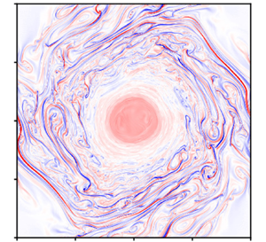
The numerical codes have been adapted directly from those used in Dritschel et al. (Reference Dritschel, Diamond and Tobias2018) for the two-dimensional limit  $L_D\to \infty$, and from the hydrodynamic shallow-water and vertically averaged codes used in Dritschel & Jalali (Reference Dritschel and Jalali2020) and Jalali & Dritschel (Reference Jalali and Dritschel2021). Without a magnetic field, the codes reproduce the results in Jalali & Dritschel (Reference Jalali and Dritschel2021) with very minor differences associated with using the linearised PV anomaly $q_l$ in place of full PV, a variable time step, and variable hyperviscosity in the present codes. (The numerical damping rate on the highest resolved wavenumber is $10(f+\zeta _{rms})$ rather than $10f$; see Appendix C in Dritschel & Jalali Reference Dritschel and Jalali2020.) Also, for large $L_D$, the shallow-water code reproduces closely the two-dimensional magnetic results of Dritschel et al. (Reference Dritschel, Diamond and Tobias2018). This is a difficult limit to simulate with a shallow-water code since short-scale gravity waves are fast ( $c=fL_D\gg U_0$), requiring a small time step for accuracy. At the same time, the Rossby number $\varepsilon$ must be small to avoid ageostrophic effects. Nonetheless, with $L_D=4$ and ${\varepsilon =0.25}$, the evolution of the vertical current density $j_z$ shown in figure 1 is strikingly similar to that shown in figure 2 (three middle panels, right column) in Dritschel et al. (Reference Dritschel, Diamond and Tobias2018) – note that the field values are a factor $\varepsilon$ smaller here. Only by the latest time are differences apparent, with the vortex rotated slightly less here, an effect due mainly to the finite value of $L_D$. The agreement is remarkable considering that $L_D$ is not particularly large, nor is $\varepsilon$ particularly small. Moreover, the vorticity-based Rossby number ${Ro}=|\zeta |_{max}/f$ rises from approximately $0.305$ to $0.884$ at late times. However, the free surface varies by no more than $0.614\,\%$, and this decays to $0.335\,\%$ by late times.
Current density field  $j_z({\boldsymbol {x}},t)$ at three scaled times $\tilde {t}=\varepsilon t$ for an MHD shallow-water simulation with $\mathfrak {g}=2$, ${\varepsilon =0.25}$ and $L_D=4$.

Current density field  $j_z({\boldsymbol {x}},t)$ at the final time $\tilde {t}=\varepsilon t=25$ for $\varepsilon =0.1$, ${L_D=0.25}$ and $\mathfrak {g}=2$; (a) regular magnetic diffusion; (b) alternative magnetic diffusion (which keeps $\boldsymbol {\nabla }\boldsymbol {\cdot }(h{\boldsymbol {B}})=0$); and (c) the difference ((b) minus (a)).

3.2. Dependence on the form of the diffusion
We start by comparing the evolution of the models with different forms of magnetic diffusion, holding all other parameters fixed. (Note that in the numerical code, the scalar potential  $A$ in (2.51) is split into a mean part $B_0 y$ and a residual $\tilde {A}$ so that the latter can be represented as a periodic field.) To produce a strong interplay between the magnetic field and the fluid motion, we choose the Rossby number $\varepsilon =0.1$, the radius of deformation ${L_D=0.25}$, and the gain $\mathfrak {g}=2$. The current density field $j_z$ at the final time ( $t=250$) is shown in figure 2, where the simulation using regular magnetic diffusion in figure 2(a) is compared to that using the alternative model of Gilbert et al. (Reference Gilbert, Griffiths and Hughes2022) in figure 2(b); the difference field is shown in figure 2(c). Qualitatively, the alternative diffusion that keeps $\boldsymbol {\nabla }\boldsymbol {\cdot }(h{\boldsymbol {B}})=0$ has little impact, even by this late time in the evolution. The overall structure and amplitude of the field are closely comparable to those found in the regular diffusion case. There are quantitative differences (see figure 2c), primarily at small scales; however, in such a complex flow, the small scales are the least predictable, so this is to be expected. Comparing the energy components in figure 3, there are hardly any visible differences between the two simulations. The kinetic energy differs the most, but still only slightly. The detailed variations of the energy components compare closely despite using different magnetic diffusion mechanisms.
(a–d) Time evolutions of the scaled total, potential, kinetic and magnetic energy, respectively, for a simulation with regular magnetic diffusion (solid curves) and a simulation with alternative magnetic diffusion (dashed curves). The flow parameters are the same as in figure 2. Note that  $\mathcal {E}_h$ is defined relative to its initial value to facilitate comparison after scaling by $\varepsilon L_D^2$. This is why this component and the total energy have negative values.

Hence we believe that the precise form of the diffusive operator has little effect on the form of the solution for these problems where the magnetic field is imposed a priori (rather than generated self-consistently via a dynamo process, where the diffusive process is key). For this reason, henceforth in this paper, we will consider the evolution of the model using regular magnetic diffusion, where the magnetic field is allowed to leave (and enter) the upper free surface.
3.3. Dependence on the Rossby deformation length
We next investigate flows for which the Rossby deformation length  $L_D$ is comparable with or smaller than the vortex radius $R$ (
$R$ ( $\approx 0.5$), and for which the free surface exhibits strong variations. Here, we consider flows in magneto-hydrostatic balance, and defer discussion of non-hydrostatic effects to § 3.5. We vary $L_D$ and $\varepsilon$ together so that the initial height anomaly field $\tilde h$ is similar in each simulation. This is done by choosing $\varepsilon =1.6L_D^2$ for three values of $L_D$: $0.5$, $0.25$ and $0.125$. This gives $\varepsilon =0.4$, $0.1$ and $0.025$, respectively. The corresponding initial minimum and maximum values of $\tilde h$ are $(-0.652,0.164)$, $(-0.604,0.161)$ and $(-0.592,0.161)$, and these values change little as the flow evolves. The initial horizontal magnetic field is specified through the gain parameter $\mathfrak {g}$, and as in figure 1, we take $\mathfrak {g}=2$.
The three simulations were carried out to the same final scaled time  $\tilde {t}=\varepsilon t=25$. The vorticity evolution is compared in figure 4 at a few characteristic times. At early times, the evolution is very similar, with a wind-up of alternating positive and negative bands of vorticity that strengthen up to approximately $t=14$ (the Rossby number ${Ro}$ climbs from just under $0.5$ to over $2.1$ when $L_D=1/2$). These bands are created largely by the effect of the Lorentz force; the initial vorticity is only slightly negative outside the vortex. The tightly wound bands then undergo instability and mix, leaving a region of near zero vorticity surrounding a central core (see also Gilbert, Mason & Tobias Reference Gilbert, Mason and Tobias2016). In the periphery, strong bands of vorticity stretch in the periodic flow field and decay gradually at late times.
Vertical vorticity field  $\zeta ({\boldsymbol {x}},t)$ at three scaled times $\tilde {t}=\varepsilon t$ for three simulations having different $L_D$ as labelled, and for $\mathfrak {g}=2$. Note that $\varepsilon =1.6L_D^2$.

As  $L_D$ decreases, the instability is less vigorous and smaller scale, yet leaves a smaller vortex core at late times. The flow is also more axisymmetric. This behaviour is consistent with the fact that flow interactions generally weaken as $L_D$ decreases. This is quantified in figure 5, which shows the Rossby number $|\zeta |_{max}/f$, and the scaled maximum horizontal magnetic field (or actual gain) $\|{\boldsymbol {B}}\|_{max}/U_0$, as functions of scaled time $\tilde {t}=\varepsilon t$ for the three simulations. The Rossby number evolves similarly in all cases, the main difference being the magnitude. There is always an initial drop as the tension in the twisting magnetic field slows the vortex rotation (elaborated in Dritschel et al. Reference Dritschel, Diamond and Tobias2018), but then there is a significant increase as current sheets form in the periphery of the vortex core. At late times, these current sheets diffuse and the vorticity weakens slightly. Regarding $\|{\boldsymbol {B}}\|_{max}/U_0$, theoretically this should reach $\mathfrak {g}=2$ when the flow is mature, but the actual gain is seen to be $0.4\mathfrak {g}$– $0.5\mathfrak {g}$. In fact, the gain parameter $\mathfrak {g}$ is only a qualitative estimate of the amplification of the magnetic field. Perhaps surprisingly, the actual gain is larger when $L_D$ is smaller, despite the weaker flow interactions occurring in this case. This may explain the reduction in the size of the vortex core as $L_D$ decreases.
Time evolutions of (a) the maximum vorticity scaled by the Coriolis frequency (i.e. Rossby number), and (b) maximum horizontal magnetic field scaled by the characteristic flow speed  $U_0$, for the three simulations illustrated in figure 4.

The current density evolution (not shown) is broadly similar to that exhibited by the vorticity in figure 4, with the exception that there is no core; the magnetic field is largely expelled from the centre, as seen previously in figure 1 and first theorised by Weiss (Reference Weiss1966) and elucidated by Moffatt & Kamkar (Reference Moffatt, Kamkar and Soward1983). On the other hand, the horizontal divergence field, shown in figure 6, exhibits very different behaviour. While it also winds up at early times, it fragments into small-scale structures that subsequently grow in scale and weaken. These structures are likely to be imbalanced inertia–gravity waves, and an especially novel feature is that these waves appear to be confined to the region of relatively weak magnetic field, and so may be suppressed by the presence of a strong magnetic field. Notably, the amplitude of  $\delta$ is much smaller than that of $\zeta$, implying that the associated divergent flow contributes relatively little to the velocity field. Moreover, it decreases in proportion to $L_D^2$ or faster at intermediate and late times.
As in figure 4 but for the horizontal divergence field  $\delta ({\boldsymbol {x}},t)$.

The energy evolution in these three flows is shown in figure 7 versus (rescaled) time  $\tilde {t}$. In the figure, the energy components are scaled by $\varepsilon L_D^2$ to enable comparison, and moreover, the initial value of the potential energy $\mathcal {E}_h(0)$ is subtracted from $\mathcal {E}_h(\tilde {t})$ (the reference value of potential energy is not important, but the construction here facilitates scaling). The total energy $\mathcal {E}$ in figure 7(a) is the sum of the (redefined) potential $\mathcal {E}_h$, kinetic $\mathcal {E}_u$ and magnetic $\mathcal {E}_b$ components; see (2.36). The initial strong growth in $\mathcal {E}_b$ is offset primarily by the decrease in $\mathcal {E}_h$, especially at small $L_D$. As $L_D$ increases, the kinetic energy $\mathcal {E}_u$ accounts for an increasing proportion of this initial energy change (notice the sharper decrease of the solid curve for $L_D=1/2$ in figure 7(c), together with the slower decrease in $\mathcal {E}_h$ in figure 7(b)). Interestingly, the greatest growth in magnetic energy $\mathcal {E}_b$ occurs for the smallest $L_D$; evidently, small $L_D$ favours a greater intensification of the magnetic field ${\boldsymbol {B}}$, which in turn leads to greater destruction of the vortex core, as seen in figure 4. At early times, the total energy $\mathcal {E}$ is conserved approximately; thereafter, $\mathcal {E}$ decays owing to both magnetic and numerical dissipation. The numerical dissipation is associated indirectly with current sheet formation, which tends to generate collocated intense vorticity sheets. These sheets subsequently stretch and thin, eventually dissipating when they reach the scale of ‘surgery’ in the numerical method (here $1/16$th of the grid scale). This dissipation is inevitable in any numerical method owing to the forward energy cascade (in spectral space) induced by the magnetic field, in particular the Lorentz force (2.44).


3.4. Dependence on the magnetic diffusivity
We next examine the dependence of the flow evolution on the magnetic diffusivity  $\eta$. We keep all other parameters the same as in the simulation featuring in figure 4(d–f) ( $L_D=1/4$, $\varepsilon =0.1$, $\mathfrak {g}=2$), and vary $\eta$, equivalent to varying the grid resolution $n_g$ in our set-up. The vorticity field $\zeta$ is compared in figure 8. Note that the initial horizontal magnetic field amplitude is varied so that $B_0\propto {Rm}^{-1/2}$ to keep the gain fixed at $\mathfrak {g}=2$, on the understanding that when the flow reaches a mature stage, $\|{\boldsymbol {B}}\|\sim \mathfrak {g}U_0$. At early times, all simulations show the characteristic spiral windup of the vorticity field (echoed by $j_z$, $\delta$ and $\gamma$, not shown). The outer core then destabilises, leading to a mixed region of weak vorticity surrounding a compact inner core. At low ${Rm}$, there is very little vorticity growth before decay at late times (mainly outside the core region). With increasing ${Rm}$, the vorticity growth becomes pronounced, especially on the periphery of the outer core. Filaments thin and intensify owing to interactions with the magnetic field (the current density $j_z$ looks closely similar apart from the absence of an inner core, not shown).
Vertical vorticity field  $\zeta ({\boldsymbol {x}},t)$ at three scaled times $\tilde {t}=\varepsilon t$ for three simulations differing in their magnetic Reynolds number ${Rm}$, as indicated. The corresponding grid resolutions are (a–c) $n_g=256$, (d–f) $n_g=512$, and (g–i) $n_g=1024$. Otherwise, the simulations are identical, with ${L_D=0.25}$, $\varepsilon =0.1$ and $\mathfrak {g}=2$.

The growth in both vorticity and maximum horizontal magnetic field strength is quantified in figure 9 for these three simulations. As expected, high  ${Rm}$ favours a strong and persistent growth in vorticity, which is caused by the emergence of current sheets (not shown). The amplification of vorticity is approximately proportional to ${Rm}$, which is the expected amplification of $j_z$ based on simple scaling arguments (Dritschel et al. Reference Dritschel, Diamond and Tobias2018). On the other hand, the actual gain in the horizontal magnetic field decreases with ${Rm}$, though it is sustained over a longer period of time before diffusive effects weaken the field. While three simulations cannot be conclusive, it appears that $\|{\boldsymbol {B}}\|_{max}/U_0$ remains finite as ${Rm}\to \infty$. However, recall that the initial magnetic field is $B_0\propto {Rm}^{-1/2}$; this goes to zero in this limit.
Time evolutions of (a) the maximum vorticity scaled by the Coriolis frequency (i.e. Rossby number, and (b) maximum horizontal magnetic field scaled by the initial maximum flow speed  $U_0$, for the three simulations illustrated in figure 8.

The total energy  $\mathcal {E}$, together with its potential $\mathcal {E}_h$, kinetic $\mathcal {E}_u$ and magnetic $\mathcal {E}_b$ components, is shown as a function of (rescaled) time $\tilde {t}$ for these three flows in figure 10. The total energy $\mathcal {E}$ is better conserved especially at early times for large ${Rm}$, as expected. The potential energy (or its difference from its initial value) exhibits a similar variation, with a slower decrease occurring for large ${Rm}$. Some of this decrease is dissipative, especially for low ${Rm}$, but some also compensates for the gain in magnetic energy $\mathcal {E}_b$. There is a similar decrease in kinetic energy $\mathcal {E}_u$, though this is smaller due to the small value of $L_D$ (here $1/4$ or approximately half of the vortex radius). The magnetic energy $\mathcal {E}_b$ initially grows from low levels as the horizontal field ${\boldsymbol {B}}$ amplifies, reaching a peak that is delayed and reduced with increasing ${Rm}$. The gain in $\mathcal {E}_b$ is largest for low ${Rm}$. Recall that the scaling of mean magnetic field applied is chosen so that the peak magnetic field in each case is comparable. However, at higher ${Rm}$, the magnetic field is confined to thinner regions (with length scale ${\propto }{Rm}^{1/2}$), so it is reasonable that the integrated energy reduces as ${Rm}$ increases.
(a–d) Time evolutions of the scaled total, potential, kinetic and magnetic energy, respectively, for the three simulations illustrated in figure 8. Note that  $\mathcal {E}_h$ is defined relative to its initial value.

3.5. Dependence on finite depth: non-hydrostatic effects
Finally, we turn to the non-hydrostatic magnetic shallow-water or ‘vertically averaged’ model derived in § 2.1 (see also § 2.3). This model extends the traditional hydrostatic shallow-water model by relaxing the long-wave approximation (necessary for the hydrostatic approximation), thereby capturing explicitly horizontal scales comparable to the mean fluid depth  $H$. We compare three simulations, varying a dimensionless frequency ratio $f/N$, where $f$ is the Coriolis frequency as before, while $N\equiv \sqrt {3g/H}$ can be thought of as a buoyancy frequency (Dritschel & Jalali Reference Dritschel and Jalali2020). The justification for this appellation is that the dispersion relation for linear waves in the hydrodynamical context then closely resembles that occurring in a three-dimensional linearly stratified fluid. Small values of $f/N$ correspond to strongly stratified flows, characteristic of large to intermediate scale atmospheric and oceanic flows, while moderate to large values of $f/N$ correspond to weakly stratified flows (for observational evidence, see Dritschel & Jalali Reference Dritschel and Jalali2020). When $f/N=1$ identically, linear inertia–gravity waves are entirely trapped; their group velocity vanishes for all wavelengths. In general, inertia–gravity wave frequencies $\omega$ lie between $f$ and $N$, with $\omega \approx f$ for the longest wavelengths, and $\omega \approx N$ for the shortest wavelengths.
Figure 11 compares, for the final time only, the vorticity  $\zeta$, divergence $\delta$, and scaled non-hydrostatic pressure $P_n=\bar {p}_n/H$ for three values of $f/N$: $1/4$, $1$ and $4$. The structure of the vorticity field is weakly dependent on $f/N$, with some variation in shape of the central core, and with the lowest extreme field values occurring for $f/N=1$. The root-mean-square vorticity varies even less, taking the values $1.027$, $1.062$ and $1.059$, respectively, for $f/N=1/4$, $1$ and $4$. This weak variation with $f/N$ is consistent with previous findings in the hydrodynamical context (Dritschel & Jalali Reference Dritschel and Jalali2020). Vorticity is dominated by the underlying balance, controlled by the relatively slow advection of PV. By contrast, both divergence and non-hydrostatic pressure vary strongly with $f/N$. Both the amplitude and spatial pattern vary considerably, especially for $P_n$, which appears to scale like $(f/N)^2$. One may also observe that $\delta$ and $P_n$ are approximately $45^\circ$ out of phase but otherwise exhibit a similar spatial pattern. The impact of $f/N$ on the evolution of the magnetic field (e.g. $j_z$, not shown) is comparably weak to that seen above for the vorticity $\zeta$.
Relative vorticity  $\zeta$, divergence $\delta$ and scaled vertically integrated non-hydrostatic pressure ${P_n=\bar {p}_n/H}$ at the final (scaled) time $\tilde {t}=\varepsilon t=25$ for three non-hydrostatic shallow-water simulations with varying $f/N$ as indicated. Here, $\mathfrak {g}=2$, ${\varepsilon =0.2}5$ and $L_D=1/2$.

Regarding energy, the impact of  $f/N$ is barely visible in comparison to that found above when varying $L_D$ in figure 7 – the weakest energy component, the magnetic energy $\mathcal {E}_b$, differs by no more than 3.5 % across $f/N$ (not shown), while the other components differ by much less than 1 %. This reflects the fact that the balanced part of the flow dominates energetically. In more turbulent flows than those studied here, the impact of $f/N$ is expected to be larger, as found previously in purely hydrodynamical flows (Dritschel & Jalali Reference Dritschel and Jalali2020), owing to greater activity (i.e. more energy) at small scales.
4. Discussion
Following the approach of Green & Naghdi (Reference Green and Naghdi1976), we have derived a non-hydrostatic shallow-water model for a layer of magnetised fluid that consistently includes finite conductivity (non-zero magnetic diffusivity). Provided that the gas pressure is negligible in the layer above, one may consider two separate models of diffusion. The first allows the magnetic field to exit the domain, and the field in the layer above transits rapidly through a series of force-free equilibria. The application of such a model may be more natural to the outer layers of astrophysical objects (see e.g. Hindle, Bushby & Rogers Reference Hindle, Bushby and Rogers2019) having a tenuous atmosphere above. The second model of diffusion confines the field to the primary fluid layer so that the upper free surface remains a magnetic flux surface, which may be a good modelling assumption for the solar tachocline (Tobias & Weiss Reference Tobias and Weiss2007). In fact, the dynamical difference between these models is exceptionally small at high  $Rm$. We note that such models (and even simpler models) have been used previously for studying the stably stratified interiors of stars.
The non-hydrostatic model discussed here gives a representation of small horizontal scales (comparable to the free-surface depth) that is more accurate than traditional shallow-water models. This may be particularly important for situations in which magnetic fields play a key role. It is well known that the presence of magnetic fields can lead to the promotion of a forward cascade, rather than the inverse cascade of quasi-two-dimensional hydrodynamics (see e.g. Seshasayanan, Benavides & Alexakis (Reference Seshasayanan, Benavides and Alexakis2014) for a discussion of the transition between the two types of behaviour). Dellar (Reference Dellar2003) has already demonstrated that the linearised form of the model presented here better replicates the dispersion properties of the full three-dimensional system for waves on a smaller scale, and that nonlinear cnoidal wave solutions exist.
The derivation of the non-hydrostatic model presented here follows Green & Naghdi (Reference Green and Naghdi1976), who pointed out that for the hydrodynamic case, all that is required is a single assumption on the horizontal velocity field – namely, that it is independent of height  $z$ in the layer; the equations then follow by vertical averaging (see also Miles & Salmon Reference Miles and Salmon1985; Jalali & Dritschel Reference Jalali and Dritschel2021). In the magnetised case, the analogous assumption is that both the velocity and the horizontal magnetic field are independent of height. The non-hydrostatic magnetised shallow-water equations, together with all of their associated conservation laws, then follow directly by vertically averaging the (inviscid) Euler and magnetic induction equations.
The total energy contained within the fluid layer is not conserved owing to magnetic diffusion. Notably, without diffusion, energy is conserved only for a magnetic field confined entirely to the fluid layer (tangent to its upper and lower surfaces). As diffusion causes the magnetic field to develop a non-zero normal component at the surfaces, inevitably energy will pass through the surfaces, as well as diffuse. This situation is common in models of the solar atmosphere (Priest Reference Priest2014).
Numerical simulations were conducted for the magneto-hydrostatic version of the model (derived assuming finite gravity wave speeds  $\sqrt {gh}$ and taking the limit $h/L\to 0$, where $L$ is a characteristic horizontal scale), as well as for the fully non-hydrostatic model. We revisited the problem of a Gaussian vortex initially within a (nearly) uniform horizontal magnetic field, studied previously in Dritschel et al. (Reference Dritschel, Diamond and Tobias2018) in the two-dimensional limit of a flat free surface.
In the hydrostatically balanced cases, finite free-surface variations in the shallow-water model and a finite Rossby number nonetheless produce results that are qualitatively similar to those in Dritschel et al. (Reference Dritschel, Diamond and Tobias2018). The most pronounced differences occur when the Rossby deformation length  $L_D=\sqrt {gH}/f$ (where $H$ is the mean fluid depth, and $f$ is the Coriolis frequency) is small compared to the initial vortex radius $R$. Then the core region around the vortex is smaller and more circular, and contains a broader region of well-mixed nearly irrotational flow. The initial magnetic field is expelled to the periphery of this region, where it exhibits current sheets and collocated vorticity sheets. In the parameter regime investigated, the divergent component of the flow is weak, and weakens in proportion to $(L_D/R)^2$.
For the non-hydrostatic model, we investigated the effects of varying the Coriolis buoyancy frequency ratio  $f/N$, where $N\equiv \sqrt {3g/H}$ depends on the mean depth $H$. Perhaps as expected, whilst the vorticity (dominated by the underlying balance) is relatively insensitive to the frequency ratio, the divergence and non-hydrostatic pressure are strongly affected by changes in this ratio, exhibiting energy on smaller scales as $f/N$ increases, which may be the signature of magneto-inertia–gravity waves. We note that a greater impact of $f/N$ is likely to occur in fully turbulent flows due to heightened small-scale activity; this is worth investigating further.
We believe that the model may be used to study general features of the solar tachocline, including free-surface and non-hydrostatic effects, exploring the properties and behaviour of linear and nonlinear waves (Rossby, gravity, Alfvén). Finally, an extension to spherical geometry will enable the investigation of global instabilities and MHD turbulence in thin spherical shells, which will provide better models of the solar tachocline and the stability of jets in exoplanetary atmospheres.
Acknowledgements
We would like to acknowledge useful discussions with R. Keppens and T. Neukirch.
Funding
D.G.D. would like to thank the Leverhulme Trust for support received during a Research Fellowship. S.M.T. was supported by funding from the European Research Council (ERC) under the EU's Horizon 2020 research and innovation programme (grant agreement D5S-DLV-786780).
Declaration of interests
The authors report no conflict of interest.
Appendix A. Approximately force-free fields in the upper layer
In this appendix, we describe the circumstances under which the magnetic field in the upper layer may be considered to be a quasi-static force-free field.
In each layer, we consider the dimensional incompressible inviscid momentum equation in a rotating Cartesian frame with gravity pointing downwards, i.e.
 \begin{equation} \rho \left(\frac{{\rm D}{{\boldsymbol{u}}}}{{\rm D}{t}} + 2 \boldsymbol{\varOmega} \times{\boldsymbol{u}} \right) ={-} \boldsymbol{\nabla}{p} + {\boldsymbol{j}}\times{\boldsymbol{B}} + \rho{\boldsymbol{g}}, \end{equation}
where  $\boldsymbol {\varOmega }=\varOmega {\boldsymbol {k}}$ and ${\boldsymbol {g}}=-g{\boldsymbol {k}}$. We consider an upper layer with density $\rho _u$, and a middle, primary, fluid layer with density $\rho _l$, and take $\rho _u \ll \rho _l$ such that $\rho _u/\rho _l = \epsilon ^2$, with $\epsilon \ll 1$. We non-dimensionalise the equations using typical values of the density, fluid pressure, magnetic field and velocity in the middle layer. That is, we set $\rho = \rho _l \hat {\rho }$, $p=p_l \hat {p}$, ${\boldsymbol {B}} = B_l \hat {{\boldsymbol {B}}}$ and ${\boldsymbol {j}} = (B_l/ \mu L)\,\boldsymbol {\nabla }\times \hat {{\boldsymbol {B}}}$, where $L$ is a typical horizontal length scale. We also set ${\boldsymbol {u}} = U_l \hat {{\boldsymbol {u}}}$ and use the advective time scale $T=L/U_l$, taking $t=T\hat {t}$.
On dropping the hats, this leads to the non-dimensional inviscid momentum equation
 \begin{equation} {Ma}^2\,\frac{{\rm D}{{\boldsymbol{u}}}}{{\rm D}{t}} + \frac{{Ma}^2}{Ro}\,{\boldsymbol{k}} \times {\boldsymbol{u}} ={-} \frac{\beta}{2}\,\boldsymbol{\nabla}{p} + (\boldsymbol{\nabla}\times {\boldsymbol{B}}) \times {\boldsymbol{B}} - \frac{{Ma}^2}{{Fr}^2}\,{\boldsymbol{k}}, \end{equation}
in which
 \begin{equation} {Ma} = \frac{U_l}{v_{A,l}} = \frac{U_l \sqrt{\mu \rho_l}}{B_l} \end{equation}
is the Alfvén Mach number, where  $v_{A,l}=B_l/\sqrt {\mu \rho _l}$ is the Alfvén speed in the middle layer. Moreover,
 \begin{equation} {Ro} = \frac{U_l}{2\varOmega L},\quad {Fr} = \frac{U_l}{(g L)^{1/2}},\quad \beta = \frac{p_l}{B_l^2/ 2 \mu} \end{equation}
are, respectively, the Rossby number, the Froude number, and the plasma beta (i.e. the ratio of the fluid pressure to the magnetic pressure) in the middle layer.
With this non-dimensionalisation, the magnetic induction equation in the middle layer becomes
 \begin{equation} \frac{\partial {\boldsymbol{B}}}{\partial t} = \boldsymbol{\nabla}\times \left({\boldsymbol{u}} \times {\boldsymbol{B}}\right) + \frac{1}{Rm}\,\nabla^2 {\boldsymbol{B}}, \end{equation}
where
 \begin{equation} {Rm} = \mu \sigma_l U_l L =\frac{U_l L}{\eta_l} \end{equation}
is the magnetic Reynolds number. Here,  $\sigma _l$ is the conductivity in the middle layer, while $\eta _l = 1/(\mu \sigma _l)$ is the magnetic diffusivity.
In the upper layer, as discussed above, both the density  $\rho _u$ and the fluid pressure $p$ are small compared with their values at the bottom of the middle layer. As we will see in Appendix B, it is appropriate to assume that the magnetic field in the upper layer is of the same order as that in the middle layer, so the Alfvén speed $v_{A,u}=B_l/\sqrt {\mu \rho _u}$ is much larger in the upper layer than in the middle layer (indeed, by a factor $\epsilon ^{-1}$). In addition, we assume that the fluid pressure is small compared to the magnetic pressure in the upper layer. With $\rho _u/\rho _l = \epsilon ^2$, the equations in the upper layer become
 \begin{equation} \epsilon^2\,{Ma}^2\,\frac{{\rm D}{{\boldsymbol{u}}}}{{\rm D}{t}} + \epsilon^2\,\frac{{Ma}^2}{Ro}\,{\boldsymbol{k}} \times {\boldsymbol{u}} ={-} \frac{\beta}{2}\,\boldsymbol{\nabla}{p} + (\boldsymbol{\nabla}\times {\boldsymbol{B}}) \times {\boldsymbol{B}} - \epsilon^2\,\frac{{Ma}^2}{{Fr}^2}\,{\boldsymbol{k}}. \end{equation}
To leading order, the equation becomes one of magneto-hydrostatic balance:
 \begin{equation} 0 ={-} \frac{\beta}{2}\,\boldsymbol{\nabla}{p} + (\boldsymbol{\nabla}\times {\boldsymbol{B}}) \times {\boldsymbol{B}}. \end{equation}
Here, recall that  $p$ is the upper layer fluid pressure scaled on the characteristic middle-layer fluid pressure $p_l$. If $p_u$ is a characteristic upper layer fluid pressure, then $p$ in (A8) is of order $p_u/p_l$. Assuming that this scales like $\rho _u/\rho _l$ (as in air over water), we have $p\sim \epsilon ^2$. Thus when $\beta \epsilon ^2\ll 1$, the magnetic field adjusts to approximately satisfy the force-free condition
 \begin{equation} 0 \approx (\boldsymbol{\nabla}\times {\boldsymbol{B}}) \times {\boldsymbol{B}}. \end{equation}
Physically, because the Alfvén speed in the upper layer is much larger than a typical velocity in the middle layer, the magnetic field in the upper layer responds on a short time scale compared with the typical time scale for the evolution of the magnetic field and velocity in the middle layer. This results in the magnetic field stepping through a series of quasi-static force-free configurations as the flow below evolves (see e.g. Priest Reference Priest2014). Note that the fluid pressure in many situations is believed to be too small to act back on the layer below – just as in the hydrodynamic case. We note that Rogers & Komacek (Reference Rogers and Komacek2014) solve anelastic equations in a spherical shell and match to a potential field in the region external to the spherical shell; this is a solution to  ${\boldsymbol {j}}={\boldsymbol {0}}$, which is clearly a force-free solution.
Appendix B. Boundary and interface conditions
In this appendix, we consider the conditions that pertain at the free surface interface and the lower fixed boundary.
Without a magnetic field, the only boundary conditions are that (a) the vertical velocity  $w$ vanishes at $z=0$, (b) the free surface at $z=h$ moves with the fluid (it is a material surface consisting always of the same fluid particles), and (c) the pressure $p$ is constant at $z=h$. Condition (b) leads to an evolution equation for $h$:
$h$:
 \begin{equation} \frac{{\rm D}{(z-h)}}{{\rm D}{t}}=0 \quad\Rightarrow\quad \frac{\partial{h}}{\partial{t}}+u\,\frac{\partial{h}}{\partial{x}}+v\,\frac{\partial{h}}{\partial{y}}=w(x,y,h,t). \end{equation}
Condition (c) expresses continuity of pressure because when  ${\boldsymbol {B}}={\boldsymbol {0}}$, (A8) reduces to ${\boldsymbol {\nabla }{p}={\boldsymbol {0}}}$ in the upper layer, i.e. $p$ is a constant. In an incompressible fluid, we can take this constant to be zero without loss of generality.
For the magnetic case, we consider the lower boundary to be perfectly conducting; in this case, surface currents at the boundary are allowed. If the layer below is also static, then a trapped unchanging magnetic field is allowed there. If this magnetic field is assumed zero, then the requirement of no normal flow across the boundary yields  ${\boldsymbol {B}} \boldsymbol {\cdot } {\boldsymbol {n}} = 0$ and ${\boldsymbol {j}} \times {\boldsymbol {n}} = {\boldsymbol {0}}$ at the interface, where ${\boldsymbol {n}}$ is the unit normal vector (Jones Reference Jones2008; Gilbert et al. Reference Gilbert, Griffiths and Hughes2022).
There are two potential choices for the magnetic layer above the active (primary) layer. If the upper layer is also perfectly conducting, then again the normal field at the free surface is zero, and this field must remain tangent to the surface. This can be ensured only if one employs a special (non-ohmic) dissipation operator that is compatible with this constraint (Gilbert et al. Reference Gilbert, Griffiths and Hughes2022). This is the diffusion operator considered in (2.49). Otherwise, for finite conductivity, we must deal with the boundary conditions that apply at the free surface. Here, we consider the case where the magnetic permeability  $\mu$ of the two layers is constant. This implies that ${\boldsymbol {B}}$ is continuous at the interface, or that
 \begin{equation} \left[ {\boldsymbol{B}} \right] = {\boldsymbol{0}}, \end{equation}
where  $[\,f ]$ is the jump in the function $f$ across the interface. This implies that ${\boldsymbol {B}}$ in the upper layer should be of the same order of magnitude as that in the middle layer. Similarly, $\mu$ being constant implies that $\boldsymbol {\nabla }\boldsymbol {\cdot } {\boldsymbol {j}} = 0$ and hence
 \begin{equation} [\,\boldsymbol{j} \boldsymbol{\cdot} {\boldsymbol{n}}] = 0. \end{equation}
(This may also be derived from the integral form of Ampère's law.) While the normal current is continuous, the tangential current is not; however, the tangential electric field  ${\boldsymbol {E}}$ is, so
 \begin{equation} \left[ {\boldsymbol{E}} \times {\boldsymbol{n}} \right] = {\boldsymbol{0}}. \end{equation}
Using Ohm's law in the two regions, this is equivalent to
 \begin{equation} [ (\,\boldsymbol{j}/\sigma - {\boldsymbol{u}} \times {\boldsymbol{B}} ) \times {\boldsymbol{n}}] = {\boldsymbol{0}}. \end{equation}
Hence, given  ${\boldsymbol {u}}$, ${\boldsymbol {B}}$ (and thus ${\boldsymbol {j}}$) and $\sigma$ in the middle layer, and ${\boldsymbol {B}}$, ${\boldsymbol {j}}$ and $\sigma$ in the upper layer, it is possible to calculate the tangential components of ${\boldsymbol {u}}$ just above the interface, provided that ${\boldsymbol {B}}\boldsymbol {\cdot }{\boldsymbol {n}}=B_\perp \ne 0$, as shown next.
This calculation proceeds from (B5) as follows. We note that (B2) ensures the continuity of  ${\boldsymbol {B}}$, and we also know
 \begin{equation} [ {\boldsymbol{u}} \boldsymbol{\cdot} {\boldsymbol{n}} ] = 0. \end{equation}
Using the formula for the vector triple product in (B5) yields
 \begin{equation} [\,\boldsymbol{j}\times{\boldsymbol{n}}/\sigma + ({\boldsymbol{n}} \boldsymbol{\cdot} {\boldsymbol{B}}) {\boldsymbol{u}} -({\boldsymbol{n}} \boldsymbol{\cdot} {\boldsymbol{u}}) {\boldsymbol{B}}] = {\boldsymbol{0}}. \end{equation}
The normal component of this is zero, while the tangential components yield
 \begin{equation} [\,\boldsymbol{j}_{{\parallel}}\times{\boldsymbol{n}}/\sigma + B_\perp {\boldsymbol{u}}_{{\parallel}}] = {\boldsymbol{0}}, \end{equation}
thus providing  ${\boldsymbol {u}}_{\parallel }\equiv {\boldsymbol {u}}-({\boldsymbol {n}}\boldsymbol {\cdot }{\boldsymbol {u}}){\boldsymbol {n}}$ above the interface – though this is not needed. (Here, we have used ${\boldsymbol {j}}={\boldsymbol {j}}_{\parallel }+j_\perp {\boldsymbol {n}}$.) Note that if $B_\perp = 0$ and $\sigma$ is continuous, then ${\boldsymbol {j}}_{\parallel }$ is also continuous.
Though it is not necessary for our purposes, there are many methods for calculating nonlinear force-free fields in a domain for a given magnetic field and current at the lower boundary. Although there are some questions about the regularity and uniqueness of the solutions, successful implementations of magneto-frictional methods have been described, and more sophisticated methods have considered the case of pressure gradients and gravity (see e.g. Beliën et al. Reference Beliën, Botchev, Goedbloed, van der Holst and Keppens2002; Guo et al. Reference Guo, Xia, Keppens and Valori2016; Wiegelmann & Sakurai Reference Wiegelmann and Sakurai2021).
The remaining condition on the interface arises from continuity of the normal stress. In an inviscid fluid, this implies
 \begin{equation} \left[{-}p {\boldsymbol{n}} - \frac{|{\boldsymbol{B}}|^2}{2 \mu}\,{\boldsymbol{n}} + \frac{B_\perp {\boldsymbol{B}}}{\mu} \right] = {\boldsymbol{0}}. \end{equation}
As  ${\boldsymbol {B}}$ and $\mu$ are continuous, this means that the pressure $p$ must also be continuous.
Appendix C. The evolution of the normal component of the magnetic field at the free surface
In this appendix, we determine the evolution equation for the normal component of the magnetic field  $B_\perp = {\boldsymbol {B}}_3 \boldsymbol {\cdot } {{\boldsymbol {n}}}$.
With  ${\boldsymbol {n}} =-\boldsymbol {\nabla }{h}+{\boldsymbol {k}}$ and ${\boldsymbol {B}}_3 = {\boldsymbol {B}}-z\tau {\boldsymbol {k}}$, we have
 \begin{align} B_\perp &= {\boldsymbol{B}}_3 \boldsymbol{\cdot} {{\boldsymbol{n}}} \nonumber\\ &={-}B_x\,\frac{\partial h}{\partial x} -B_y\, \frac{\partial h}{\partial y} - h \tau \nonumber\\ &={-}\boldsymbol{\nabla}\boldsymbol{\cdot} (h {\boldsymbol{B}}). \end{align}
Note here that  ${\boldsymbol {n}}$ is not normalised. Nonetheless, ${\boldsymbol {n}}$ points normal to the surface $z=h$, and the adopted form of $B_\perp$ yields a simple evolution equation.
This equation is derived by multiplying (2.30) by  ${\boldsymbol {B}}$ and adding to (2.29) multiplied by $h$. On taking the divergence, one finds (after an overall change in sign)
 \begin{equation} \frac{\partial{B_\perp}}{\partial{t}} + \boldsymbol{\nabla}\boldsymbol{\cdot}(B_\perp{\boldsymbol{u}}) ={-}\eta\,\boldsymbol{\nabla}\boldsymbol{\cdot}(h\,\nabla^2{\boldsymbol{B}}). \end{equation}
This shows that  $B_\perp$ does not generally remain zero if initially so. The diffusive term cannot be expressed solely in terms of $B_\perp$.


 Open access

