





1. Introduction
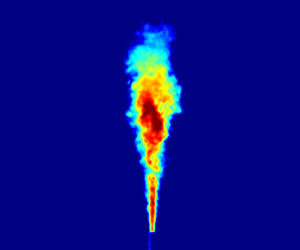
Axisymmetric jets and plumes occur when a turbulent flow exits a round source into a homogeneous (non-stratified) quiescent environment. If the density of the flow is equal to that of the ambient, then we refer to this as a neutral jet (J). If there is a density difference between the flow and ambient, then there will also be a buoyancy force, which, in the case of a vertically aligned source, may either be in the same or opposite direction to the axial momentum. When it is in the same direction as the flow, then we call this a positively buoyant jet (PBJ), whereas negatively buoyant jets (NBJs) occur when the buoyancy opposes the momentum. Both these flows can be characterised by their local Richardson number,  $Ri$, the ratio of buoyancy to momentum, where $Ri>0$ in PBJs and $Ri<0$ in NBJs. Pure plumes are a similar axisymmetric free shear flow, but where $Ri$ is constant and positive everywhere. In the far field, all PBJs approach this state (Fischer et al. Reference Fischer, List, Koh, Imberger and Brooks1979).
Jets and PBJs have a similar ‘jet-like’ structure, where they expand as they entrain ambient fluid, have Gaussian mean velocity and scalar profiles, and eventually reach a state of self-similarity in the far field (Papanicolaou & List Reference Papanicolaou and List1988; Panchapakesan & Lumley Reference Panchapakesan and Lumley1993; Wang & Law Reference Wang and Law2002; van Reeuwijk et al. Reference van Reeuwijk, Salizzoni, Hunt and Craske2016). NBJs, which have initially positive momentum but negative buoyancy, will rise if ejected vertically upwards with their momentum flux reducing with height due to their opposing buoyancy until the flow stagnates. After this, the flow reverses direction and collapses back onto itself, mixing with the opposing fluid and forming a fountain. The initial stage, before the return flow is formed, is what we refer to as an NBJ. This has a similar structure to jets/PBJs and also has Gaussian velocity/scalar profiles (Milton-McGurk et al. Reference Milton-McGurk, Williamson, Armfield and Kirkpatrick2020, Reference Milton-McGurk, Williamson, Arfmfield, Kirkpatrick and Talluru2021, Reference Milton-McGurk, Williamson, Armfield and Kirkpatrick2022; Talluru et al. Reference Talluru, Armfield, Williamson, Kirkpatrick and Milton-McGurk2021).
By invoking the conservation of mass and momentum, and assuming that the mean velocity and scalar (or buoyancy) profiles are self-similar and Gaussian, previous studies have derived analytical expressions for the mean radial velocity,  $\bar {u}$, and Reynolds stress, $\overline {w'u'}$, profiles for the case of a neutral jet and plume (Mih Reference Mih1989; Agrawal & Prasad Reference Agrawal and Prasad2003). This is possible by making use of the ‘entrainment assumption’, that the radial velocity of fluid entrained into the jet/plume is proportional to a characteristic velocity at that height by an entrainment coefficient, $\alpha$ (Morton, Taylor & Turner Reference Morton, Taylor and Turner1956). In pure jets and plumes, $\alpha$ is constant with values reported in the literature in the ranges $0.065\lesssim \alpha _j\lesssim 0.080$ and $0.10\lesssim \alpha _p\lesssim 0.16$, respectively (Fischer et al. Reference Fischer, List, Koh, Imberger and Brooks1979; Carazzo, Kaminski & Tait Reference Carazzo, Kaminski and Tait2006). The derivations of these analytical profiles make use of the decay rate of the axial velocity scale and the radial expansion rate, which arise from the conservation equations under the assumption of self-similarity, and are simple power laws in the case of pure jets and plumes (Priestley & Ball Reference Priestley and Ball1955; Morton et al. Reference Morton, Taylor and Turner1956; Rajaratnam Reference Rajaratnam1976; Fischer et al. Reference Fischer, List, Koh, Imberger and Brooks1979). For PBJs and NBJs, $\alpha$ is not constant and instead depends on the local Richardson number, $Ri$, and the velocity decay and expansion rates are not simple power laws (Morton Reference Morton1959; Fox Reference Fox1970; Kaminski, Tait & Carazzo Reference Kaminski, Tait and Carazzo2005; van Reeuwijk & Craske Reference van Reeuwijk and Craske2015; Milton-McGurk et al. Reference Milton-McGurk, Williamson, Arfmfield, Kirkpatrick and Talluru2021, Reference Milton-McGurk, Williamson, Armfield and Kirkpatrick2022). Owing to this, there has not yet been any attempt to derive analytical expressions for $\bar {u}$, $\overline {w'u'}$ or $\overline {u'b'}$ for jets with arbitrary buoyancy (e.g. PBJs or NBJs) based on the assumption of Gaussian axial velocity profiles. This is the purpose of the present study, which will use analytical expressions for $\alpha$ and the velocity decay/expansion rates to derive these expressions and compare them to measurements from our previous work (Milton-McGurk et al. Reference Milton-McGurk, Williamson, Arfmfield, Kirkpatrick and Talluru2021), as well as other experimental and numerical data in the literature (Wang & Law Reference Wang and Law2002; Darisse, Lemay & Benaïssa Reference Darisse, Lemay and Benaïssa2013; van Reeuwijk et al. Reference van Reeuwijk, Salizzoni, Hunt and Craske2016).
2. Governing equations
For a high-Reynolds-number, statistically axisymmetric flow in a homogeneous environment, and invoking the Boussinesq approximation, the conservation of volume, axial momentum, buoyancy and axial kinetic energy are
 $$\begin{gather} \frac{\partial}{\partial r}\left(r\bar{u}\right) + \frac{\partial}{\partial z}\left(r\bar{w}\right) = 0, \end{gather}$$
 $$\begin{gather}\frac{\partial}{\partial r}\left(r\bar{u}\bar{w}+r\overline{u'w'}\right) + \frac{\partial}{\partial z}\left(r\bar{w}^2\right) = r\bar{b}, \end{gather}$$
 $$\begin{gather}\frac{\partial}{\partial r}\left(r\bar{u}\bar{b} + r\overline{u'b'}\right) + \frac{\partial}{\partial z}\left(r\bar{w}\bar{b}\right) = 0, \end{gather}$$
 $$\begin{gather}\frac{\partial}{\partial r}\left(r\bar{u}\bar{w}^2+2r\overline{u'w'}\bar{w}\right) + \frac{\partial}{\partial z}\left(r\bar{w}^3\right) =2r\overline{u'w'}\frac{\partial\bar{w}}{\partial r} + 2r\bar{w}\bar{b}, \end{gather}$$
where all pressure terms, and higher-order turbulence contributions involving  $\overline {w'b'}$ and $\overline {w'^2}$, are neglected (Kaminski et al. Reference Kaminski, Tait and Carazzo2005; van Reeuwijk & Craske Reference van Reeuwijk and Craske2015). Here $w=w(r,\phi,z)$ and $u=u(r,\phi,z)$ are the instantaneous axial and radial velocities corresponding to coordinates $z$ and $r$, respectively, and $b=g{\rm \Delta} \rho /\rho _a$ is the buoyancy. The azimuthal component, $\phi$, disappears when averaging because the flow is assumed to be axisymmetric, and so we have $\bar {w}=\bar {w}(r,z)$, $\bar {b}=\bar {b}(r,z)$, etc. The gravitational acceleration is denoted by $g$ and ${\rm \Delta} \rho$ is the difference between the local and ambient density, $\rho _a$. For NBJs, ${\rm \Delta} \rho <0$, whereas ${\rm \Delta} \rho >0$ in PBJs and plumes. The buoyancy and scalar concentration are related by a constant such that $b=c{\rm \Delta} \rho _o g/\rho _a$, where ${\rm \Delta} \rho _o$ is the density difference between the plume/jet with the ambient at the source. All instantaneous quantities may be decomposed into their mean and fluctuating components, e.g. $w=\bar {w}+w'$.
The fluxes of volume, momentum, buoyancy and integral buoyancy,  $Q$,
$Q$,  $M$,
$M$,  $F$ and $B$, may be defined from the mean velocity and buoyancy profiles,
 \begin{align} Q = 2\int_{0}^{\infty}\bar{w}r\,\mathrm{d}r,\quad M = 2\int_{0}^{\infty}\bar{w}^2r\,\mathrm{d}r,\quad F = 2\int_{0}^{\infty}\bar{w}\bar{b}r\,\mathrm{d}r,\quad B = 2\int_{0}^{\infty}\bar{b}r\,\mathrm{d}r, \end{align}
which have been scaled to remove a factor of  ${\rm \pi}$. These allow local velocity, length and buoyancy scales to be defined,
 \begin{equation} w_m = \frac{M}{Q}, \quad r_m = \frac{Q}{M^{1/2}}, \quad b_m = \frac{BM}{Q^2}, \end{equation}
as well as the local Richardson number,
 \begin{equation} Ri = \frac{b_mr_m}{w_m^2}. \end{equation}
Equations (2.1)–(2.4) may then be integrated with respect to  $r$ from zero to infinity to obtain the following system of ordinary differential equations (ODEs),
 $$\begin{gather} \frac{\mathrm{d}Q}{\mathrm{d}z} = 2\alpha M^{1/2} \end{gather}$$
 $$\begin{gather}\frac{\mathrm{d}M}{\mathrm{d}z} = B = \frac{FQ}{\theta_mM} \end{gather}$$
 $$\begin{gather}\frac{\mathrm{d}F}{\mathrm{d}z} = 0 \end{gather}$$
 $$\begin{gather}\frac{\mathrm{d}}{\mathrm{d}z}\left(\gamma_m\frac{M^2}{Q}\right) = \delta_m\frac{M^{5/2}}{Q^2} + 2F, \end{gather}$$
where the entrainment coefficient,  $\alpha$, is defined as
 \begin{equation} \left(r\bar{u}\right)_{r=\infty} ={-}\alpha r_m w_m. \end{equation}
The quantities  $\theta _m$, $\gamma _m$ and $\delta _m$ are referred to as the ‘profile coefficients’, and can be interpreted as the dimensionless buoyancy flux, mean kinetic energy and turbulence production,
 \begin{equation} \left. \begin{array}{l} \displaystyle \theta_m=\dfrac{F}{w_mb_mr_m^2}, \\ \displaystyle \gamma_m=\dfrac{2}{w_m^3r_m^2}\int_{0}^{\infty}\bar{w}^3 r\,\mathrm{d}r, \\ \displaystyle \delta_m=\dfrac{4}{w_m^3r_m}\int_{0}^{\infty}\overline{w'u'} \dfrac{\partial\bar{w}}{\partial r}r\,\mathrm{d}r. \end{array}\right\} \end{equation}
 By combining (2.8), (2.9) and (2.11), van Reeuwijk & Craske (Reference van Reeuwijk and Craske2015) derived the following expression for  $\alpha$, which makes no assumptions about the shape of the profiles but assumes they are self-similar,
 \begin{equation} \alpha ={-}\frac{\delta_m}{2\gamma_m} + \left(1-\frac{\theta_m}{\gamma_m}\right)Ri \end{equation}
as well as the following equation for the spreading rate,
 \begin{equation} \frac{\mathrm{d}r_m}{\mathrm{d}z} ={-}\frac{\delta_m}{\gamma_m} + \frac{3}{2}\left(1 - \frac{4}{3}\frac{\theta_m}{\gamma_m}\right)Ri. \end{equation}
Using a similar approach, the following expressions describing the development of the velocity and buoyancy scales may also be derived:
 $$\begin{gather} \frac{r_m}{w_m}\frac{\mathrm{d}w_m}{\mathrm{d}z} = \frac{\delta_m}{\gamma_m} + \left(\frac{2\theta_m}{\gamma_m}-1\right)Ri, \end{gather}$$
 $$\begin{gather}\frac{r_m}{b_m}\frac{\mathrm{d}b_m}{\mathrm{d}z} = \frac{\delta_m}{\gamma_m} - 2\left(1-\frac{\theta_m}{\gamma_m}\right)Ri ={-}2\alpha. \end{gather}$$
 By invoking the assumption of self-similar Gaussian mean velocity and buoyancy profiles, several additional simplifications can be made. For instance, let the velocity and buoyancy profiles be described by the shape functions  $f$ and $y$, respectively,
 $$\begin{gather} \bar{w}(r,z) = 2w_m f(\eta) , \end{gather}$$
 $$\begin{gather}\bar{b}(r,z) = \frac{2b_m}{\lambda^2}y(\eta), \end{gather}$$
where  $\eta =\sqrt {2}r/r_m$ and $\lambda$ is the ratio of $1/e$ widths of the buoyancy and velocity profiles, $r_b$ and $r_w$,
 \begin{equation} \lambda = \frac{r_b}{r_w}. \end{equation}
We then set
 $$\begin{gather} f(\eta) = {\rm e}^{-\eta^2}, \end{gather}$$
 $$\begin{gather}y(\eta) = \exp({-\eta^2/\lambda^2}), \end{gather}$$
which is equivalent to assuming Gaussian mean velocity and buoyancy profiles that have centreline values  $\bar {w}_c=2w_m$ and $\overline {b}_c=2b_m/\lambda ^2$, and $1/e$ widths $r_w=r_m/\sqrt {2}$ and $r_b=\lambda r_m/\sqrt {2}$. By evaluating the definitions of the profile coefficients in (2.13), we then have
 \begin{equation} \theta_m=\frac{2}{\lambda^2+1},\quad \gamma_m=\frac{4}{3}. \end{equation}
The entrainment coefficient,  $\alpha$ in (2.14), therefore depends only on $\delta _m$, $\lambda$ and $Ri$.
$Ri$.
For fully self-similar flows, such as pure jets ( $Ri=0$) and plumes ( $Ri=\textrm {constant}$) in the far field, all profile coefficients are constant. This assumption of self-similarity, along with the conservation equations (2.1)–(2.4) (or a simple dimensional analysis), leads to $w_m\sim z^{-1}$ and $w_m\sim z^{-1/3}$ in pure jets and plumes, respectively, and $r_m\sim z$ in both (Priestley & Ball Reference Priestley and Ball1955; Morton et al. Reference Morton, Taylor and Turner1956; Rajaratnam Reference Rajaratnam1976; Fischer et al. Reference Fischer, List, Koh, Imberger and Brooks1979). Previous studies have used these results to derive analytical expressions for $\bar {u}$, $\overline {w'u'}$ and $\overline {u'b'}$ for these limiting cases by assuming Gaussian mean profiles (Mih Reference Mih1989; Agrawal & Prasad Reference Agrawal and Prasad2003). The following sections will instead use (2.14)–(2.17) to derive expressions for these profiles in terms of the profile coefficients in (2.13). Although these assumptions are more questionable in PBJs and NBJs, we argue that, provided appropriate values of $\lambda$ and $\delta _m$ are used for a given $Ri$, they are still reasonable approximations and lead to predictions consistent with existing experimental and numerical data. The expressions will therefore be applicable to turbulent jets with arbitrary buoyancy, rather than only the limiting cases of pure jets and plumes.
3. Analytical expressions for profiles
3.1. Radial velocity
Let the mean radial velocity profile be described by shape function,  $h(\eta )$, such that
 \begin{equation} \bar{u}(r,z) = 2w_m h(\eta) . \end{equation}
By inserting this into the continuity equation (2.1), and using (2.18) and (2.21), the following expression for the shape of the radial velocity profile may be derived:
 \begin{equation} h = \frac{\sqrt{2}}{2\eta}\left({\rm e}^{-\eta^2} \left(\eta^2\frac{\mathrm{d}r_m}{\mathrm{d}z} + \alpha\right) - \alpha \right). \end{equation}
By substituting the equations for  $\mathrm {d}r_m/\mathrm {d}z$ and $\alpha$ into (2.15) and (2.14), the following is obtained:
 \begin{equation} h = \frac{\sqrt{2}}{2\eta}\left({\rm e}^{-\eta^2}\left[-\frac{3}{4}\delta_m \left(\eta^2+\frac{1}{2}\right) + \left(\frac{3}{2}\left(1-\theta_m\right) \eta^2+1-\frac{3}{4}\theta_m\right)Ri \right] - \alpha \right). \end{equation}
 Provided  $\bar {w}$ can be described by a Gaussian profile, this is valid for self-similar axisymmetric turbulent jets with arbitrary buoyancy, and is consistent with previously derived expressions for the limiting cases of pure jets/plumes (Mih Reference Mih1989; Agrawal & Prasad Reference Agrawal and Prasad2003). By using the expression for $\alpha$ in (2.14), and observing (2.23a,b), this equation for $h$ depends only on $\lambda$, $\delta _m$ and $Ri$.
$Ri$.
3.2. Reynolds stress
Let the self-similar Reynolds stress profile be written in terms of shape function  $j(\eta )$,
 \begin{equation} \overline{w'u'}(r,z) = 4w_m^2 j(\eta). \end{equation}
This can be substituted for  $\overline {w'u'}$ in the momentum equation, (2.2), along with shape functions (2.18), (2.19) and (3.1) for $\bar {w}$, $\bar {b}$ and $\bar {u}$, to derive
 \begin{equation} \frac{\partial}{\partial \eta}\left(\eta j\right) = \sqrt{2}\eta^2 f \frac{\textrm{d}r_m}{\textrm{d}z}\frac{\partial f}{\partial \eta} - \sqrt{2}\eta f^2 \frac{r_m}{w_m}\frac{\textrm{d}w_m}{\textrm{d}z} - \frac{\partial}{\partial \eta}\left(\eta f h\right) \frac{Ri\sqrt{2}}{4\lambda^2}y\eta, \end{equation}
after performing a change of variables to express the partial derivatives in terms of  $\eta$ instead of $r$ and $z$. By substituting the Gaussian functions in (2.21) and (2.22) for $f$ and $y$, this may be integrated with respect to $\eta$ to give
 \begin{align} j &= \frac{\sqrt{2}}{4\eta}\left(\frac{\mathrm{d}r_m}{\mathrm{d}z} \left[\exp({-2\eta^2})(2\eta^2+1)-1\right] + \frac{r_m}{w_m} \frac{\mathrm{d}w_m}{\mathrm{d}z}\left(\exp({-2\eta^2})-1\right) \right.\nonumber\\ &\quad \left.+\frac{Ri}{2}\left(1-\exp({-\eta^2/\lambda^2})\right)\right) - {\rm e}^{-\eta^2}h, \end{align}
where the constant of integration is obtained by considering the limit as  $\eta \rightarrow 0$ and assuming that $\overline {w'u'}$ is bounded at $\eta =0$ (Agrawal & Prasad Reference Agrawal and Prasad2003). The following may then by obtained by inserting (2.15) and (2.16), and using the derived expression for $h$,
$h$,
 \begin{equation} j = \frac{\sqrt{2}}{2\eta}\left(\alpha \,{\rm e}^{-\eta^2} - \exp({-2\eta^2}) \left[-\frac{3}{8}\delta_m+\frac{3}{4}\left(1-\theta_m\right)Ri\right] -\frac{Ri}{4}\exp({-\eta^2/\lambda^2})\right). \end{equation}
3.3. Radial scalar flux
Now consider the shape function,  $p$, corresponding to the radial scalar flux profile,
 \begin{equation} \overline{u'b'} = \frac{4w_mb_m}{\lambda^2}p(\eta). \end{equation}
By inserting (3.8) into the conservation of buoyancy equation (2.3), and using the expression for  $h$ in (3.2) and $\mathrm {d}b_m/\mathrm {d}z$ in (2.17), the following may be derived:
 \begin{equation} p = \frac{\sqrt{2}}{2\eta}\alpha \exp({-\eta^2/\lambda^2})\left(1 - {\rm e}^{-\eta^2}\right). \end{equation}
4. Comparisons with experimental data
The shape functions,  $h$,
$h$,  $j$ and $p$ derived in § 3 for the radial velocity, Reynolds stress and radial scalar flux profiles depend only on $\lambda$, $\delta _m$ and $Ri$. The width ratio, $\lambda$, is typically found to be constant in pure jets and plumes in the far field, with values of $\lambda _j\simeq 1.2$ and $\lambda _p\simeq 1.0$, respectively (Papanicolaou & List Reference Papanicolaou and List1988; Shabbir & George Reference Shabbir and George1994; Wang & Law Reference Wang and Law2002; Ezzamel, Salizzoni & Hunt Reference Ezzamel, Salizzoni and Hunt2015; van Reeuwijk et al. Reference van Reeuwijk, Salizzoni, Hunt and Craske2016). The value in real PBJs may vary somewhat as they develop, but approach approximately $\lambda =1.0$ in the far field as the flow approaches a pure plume-like state where $Ri\rightarrow Ri_p$ (Panchapakesan & Lumley Reference Panchapakesan and Lumley1993; Wang & Law Reference Wang and Law2002; Ezzamel et al. Reference Ezzamel, Salizzoni and Hunt2015; van Reeuwijk et al. Reference van Reeuwijk, Salizzoni, Hunt and Craske2016). In Gaussian PBJs/plumes, it was shown in Milton-McGurk et al. (Reference Milton-McGurk, Williamson, Armfield and Kirkpatrick2022) that a value of $\lambda =1$ or $1/\sqrt {2}$ is required to maintain consistency between the conservation of mass, momentum, kinetic energy, and an additionally derived $\bar {w}^3$ equation. As a value of $\lambda =1$ is consistent with both existing literature and the conservation equations, this will be used in the present study when considering PBJs and plumes. In NBJs, which do not approach a constant $Ri$ value, $\lambda$ is not constant and has been shown to increase between $1.3\lesssim \lambda \lesssim 1.5$ over $-0.03\gtrsim Ri \gtrsim -0.3$ (Milton-McGurk et al. Reference Milton-McGurk, Williamson, Arfmfield, Kirkpatrick and Talluru2021). However, reasonable velocity predictions were obtained in Milton-McGurk et al. (Reference Milton-McGurk, Williamson, Arfmfield, Kirkpatrick and Talluru2021) by assuming a constant $\lambda \simeq 1.46$, and solving an integral model of the flow.
The dimensionless turbulence production,  $\delta _m$, has been found to be approximately constant in pure jets and plumes, and although there is some variation in the literature ( $-0.23\lesssim \delta _m\lesssim -0.20$ in plumes, $-0.21\lesssim \delta _m\lesssim -0.19$ in jets), $\delta _m\simeq -0.20$ in both cases (Wang & Law Reference Wang and Law2002; Ezzamel et al. Reference Ezzamel, Salizzoni and Hunt2015; van Reeuwijk & Craske Reference van Reeuwijk and Craske2015; van Reeuwijk et al. Reference van Reeuwijk, Salizzoni, Hunt and Craske2016). van Reeuwijk et al. (Reference van Reeuwijk, Salizzoni, Hunt and Craske2016) also reported an approximately constant value in PBJs, although this was slightly lower in magnitude than the jet and plume values with $\delta _m\simeq -0.175$. In NBJs, $\delta _m$ is not constant and was found in Milton-McGurk et al. (Reference Milton-McGurk, Williamson, Arfmfield, Kirkpatrick and Talluru2021) to become increasingly negative as $Ri\rightarrow -\infty$, approximately following the linear relation,
 \begin{equation} \delta_m = \delta_j + \tilde\delta Ri. \end{equation}
Here  $\delta _j\simeq -0.2$ is the ‘neutral jet value’, and $\tilde \delta \simeq 0.604$ is an ad hoc empirical term that captures the observed variation of $\delta _m$ with $Ri$.
$Ri$.
For the remainder of this section, we use these aforementioned values of  $\delta _m$ and $\lambda$ as inputs into shape functions $h$,
$h$,  $j$ and $h$ for a given $Ri$. Although these are only approximations for the intermediate cases of PBJs and NBJs, we see that they lead to good agreement with existing data. In the case of pure jets and plumes, we have that $Ri_j=0$ and $Ri_p=8\alpha _p/5$, respectively (van Reeuwijk & Craske Reference van Reeuwijk and Craske2015). For Gaussian velocity/scalar profiles and $\lambda _p=1.0$, this leads to $\alpha _j=-3\delta _m/8$ and $\alpha _p=-5\delta _m/8$ using (2.14). Substituting these values into (3.3) and (3.7) gives equivalent expressions to those derived by Agrawal & Prasad (Reference Agrawal and Prasad2003) and Mih (Reference Mih1989). These were found to be in reasonable agreement with existing experimental data and so are not explored further here. However, the application of $h$,
$h$,  $j$ and $p$ to PBJs and NBJs, and $p$ to pure jets, has not been considered until now.
Figure 1 shows normalised  $\overline {u'c'}$ profiles for a pure jet and plume obtained from an experimental study by the previous authors (Milton-McGurk et al. Reference Milton-McGurk, Williamson, Arfmfield, Kirkpatrick and Talluru2021) (jet only), as well as direct numerical simulation (DNS) data from van Reeuwijk et al. (Reference van Reeuwijk, Salizzoni, Hunt and Craske2016), and the best fit profiles of experiments by Wang & Law (Reference Wang and Law2002). The predictions corresponding to $p$ for both flows is also shown, where $\delta _m=-0.20$ and $\lambda =1.2$ for the jet, and $\delta _m=-0.20$ and $\lambda =1.0$ for the plume. Although there is some small variation between data from the three studies, they are all in reasonable agreement with each other and $p$ for both the jet and plume cases.
The shape function  $p$, defined in (3.9), for the case of a neutral jet ( $\lambda =1.2$, $\delta _m=-0.20$) in (a), and pure plume ( $\lambda =1.0$, $\delta _m=-0.20$) in (b). The corresponding normalised radial scalar flux profiles obtained in an experimental study by the present authors (jet only) (Milton-McGurk et al. Reference Milton-McGurk, Williamson, Armfield and Kirkpatrick2020, Reference Milton-McGurk, Williamson, Arfmfield, Kirkpatrick and Talluru2021), as well as by Wang & Law (Reference Wang and Law2002) and van Reeuwijk et al. (Reference van Reeuwijk, Salizzoni, Hunt and Craske2016), are also shown.

Figure 2 shows normalised  $\bar {u}$, $\overline {w'u'}$ and $\overline {u'b'}$ profiles for a PBJ from van Reeuwijk et al. (Reference van Reeuwijk, Salizzoni, Hunt and Craske2016). Also shown are the corresponding $h$,
$h$,  $j$ and $p$ profiles with $\delta _m=-0.175$ and $\lambda =1.0$. The local $Ri$ corresponding to the profiles from van Reeuwijk et al. (Reference van Reeuwijk, Salizzoni, Hunt and Craske2016), and hence used for $h$,
$h$,  $j$ and $p$, were estimated as $Ri\simeq 0.042$ and $0.084$. Only one $Ri$ profile is shown for $\overline {w'u'}$, because for the case where $\lambda =1$, (3.7) for $j$ simplifies to a form that is not dependent on $Ri$. There is good agreement between the analytical profiles and those from van Reeuwijk et al. (Reference van Reeuwijk, Salizzoni, Hunt and Craske2016) for $\bar {u}$, $\overline {w'u'}$ and $\overline {u'b'}$ at both $Ri$ locations. Also shown are the predictions for pure jets and plumes, so that we may observe whether there is any improvement gained by using the presently derived expressions for arbitrary $Ri$. Here we set $\lambda =1$ for both cases, because this is more appropriate for PBJs than the usual $\lambda =1.2$ value for pure jets (Milton-McGurk et al. Reference Milton-McGurk, Williamson, Armfield and Kirkpatrick2022). The $p$ prediction for a J is very close to that for the $Ri=-0.042$ PBJ in figure 2(c), because, in this case, the only difference between predictions is due to $\alpha$. For $Ri=-0.042$, the flow is still quite ‘jet-like’ and so these values are similar for a PBJ ( $\alpha =0.076$) and J ( $\alpha =0.075$). For $Ri=-0.084$, the arbitrary- $Ri$ relation has considerably better agreement for $p$, which is also the case at both $Ri$ in figure 2(a) for $h$. As the Reynolds stress profile, $j$, is independent of $Ri$ when $\lambda =1$, the function is the same for pure jets/plumes/PBJs with this $\lambda$, and is therefore controlled by $\delta _m$. This value is approximately the same for jets/plumes ( $\delta _m\simeq -0.20$), and is slightly lower for PBJs ( $\delta _m\simeq -0.175$) (van Reeuwijk et al. Reference van Reeuwijk, Salizzoni, Hunt and Craske2016). The J prediction shown in figure 2(c) corresponds to $\delta _m=-0.20$, which does not have as good agreement as the PBJ prediction using $\delta _m=-0.175$.
The shape functions  $h$,
$h$,  $j$ and $p$ defined in (3.3), (3.7) and (3.9), respectively, are shown in (a)–(c) for the case of a PBJ with $\lambda =1.0$ and $\delta _m=-0.175$ at $Ri=0.042$ and $Ri=0.084$. The corresponding normalised radial velocity, Reynolds stress and radial scalar flux profiles obtained from DNS study by van Reeuwijk et al. (Reference van Reeuwijk, Salizzoni, Hunt and Craske2016) are also shown in each case. The analytical expressions for a pure jet (J) and plume (P) are also shown as a reference.

Figures 3–5 show normalised  $\bar {u}$, $\overline {w'u'}$ and $\overline {u'b'}$ profiles for an NBJ at two $Ri$ locations. These experimental data were gathered in previous studies by the present authors using combined particle image velocimetry (PIV) and planar laser-induced fluorescence (PLIF), with additional details available in Milton-McGurk et al. (Reference Milton-McGurk, Williamson, Armfield and Kirkpatrick2020) and Milton-McGurk et al. (Reference Milton-McGurk, Williamson, Arfmfield, Kirkpatrick and Talluru2021). The corresponding analytical $h$,
$h$,  $j$ and $p$ expressions are also shown, obtained by assuming a constant $\lambda =1.46$ and the linear expression for $\delta _m$ in (4.1), along with the $Ri$ value corresponding to the experimental data. Reasonable agreement is found for $h$ in figure 3, whereas $j$ and $p$ in figures 4 and 5 show excellent agreement.
The shape function  $h$, defined in (3.3), for the case of an NBJ with $\lambda =1.46$ and $\delta _m\sim Ri$ (as defined by (4.1)) at $Ri=-0.08$ in (a) and $Ri=-0.10$ in (b). The corresponding normalised radial velocity profiles obtained in an experimental study by the present authors are also shown (Milton-McGurk et al. Reference Milton-McGurk, Williamson, Armfield and Kirkpatrick2020, Reference Milton-McGurk, Williamson, Arfmfield, Kirkpatrick and Talluru2021).

The shape function  $j$, defined in (3.7), for the case of an NBJ with $\lambda =1.46$ and $\delta _m\sim Ri$ (as defined by (4.1)) at $Ri=-0.08$ in (a) and $Ri=-0.10$ in (b). The corresponding normalised Reynolds stress profiles obtained in an experimental study by the present authors are also shown (Milton-McGurk et al. Reference Milton-McGurk, Williamson, Armfield and Kirkpatrick2020, Reference Milton-McGurk, Williamson, Arfmfield, Kirkpatrick and Talluru2021).

The shape function  $p$, defined in (3.9), for the case of an NBJ with $\lambda =1.46$ and $\delta _m\sim Ri$ (as defined by (4.1)) at $Ri=-0.08$ in (a) and $Ri=-0.10$ in (b). The corresponding normalised radial scalar flux profiles obtained in an experimental study by the present authors are also shown (Milton-McGurk et al. Reference Milton-McGurk, Williamson, Armfield and Kirkpatrick2020, Reference Milton-McGurk, Williamson, Arfmfield, Kirkpatrick and Talluru2021).

At the top of an NBJ,  $w_m\rightarrow 0$ and $Ri\rightarrow -\infty$ as the mean flow velocity stagnates. After this, the flow reverses direction and eventually forms a fully developed fountain. The region where the fluid reverses direction is referred to as the ‘cap’ region, which occurs in the model by Hunt & Debugne (Reference Hunt and Debugne2016) of a fully developed fountain at $Ri=-0.5$. The present analysis and hence the $h$,
$h$,  $j$ and $p$ expressions are unlikely to be valid in NBJs near this region, where the flow is no longer jet-like (Milton-McGurk et al. Reference Milton-McGurk, Williamson, Arfmfield, Kirkpatrick and Talluru2021; Talluru, Williamson & Armfield Reference Talluru, Williamson and Armfield2022). The agreement between the profile predictions and NBJ data in figures 3–5 suggest that the locations with $Ri=-0.08$ and $-0.10$ are sufficiently far from the cap region that the present assumptions remain reasonable. However, in the NBJ data (Milton-McGurk et al. Reference Milton-McGurk, Williamson, Arfmfield, Kirkpatrick and Talluru2021), the profiles began to depart from the predictions for $Ri\lesssim -0.11$, and so the expressions may longer be valid in this region.
5. Turbulent Prandtl/Schmidt number
The derived expressions for Reynolds stress and radial scalar flux may also be used to obtain an expression for the turbulent Schmidt number,  $Sc_T$,
 \begin{equation} Sc_T = \frac{\nu_T}{\kappa_T}, \end{equation}
where  $\nu _T$ and $\kappa _T$ are the momentum and mass diffusivities, respectively,
 \begin{equation} \nu_T ={-}\frac{\overline{w'u'}}{\partial\bar{w}/\partial r},\quad \kappa_T ={-}\frac{\overline{u'b'}}{\partial\bar{b}/\partial r}. \end{equation}
As the experiments reported in Milton-McGurk et al. (Reference Milton-McGurk, Williamson, Armfield and Kirkpatrick2020, Reference Milton-McGurk, Williamson, Arfmfield, Kirkpatrick and Talluru2021) used saline as the scalar tracer, we use the turbulent Schmidt number here rather than the turbulent Prandtl number,  $Pr_T$. The same expressions also apply to $Pr_T$, except $\kappa _T$ would instead refer to thermal diffusivity. By using (3.7) and (3.9) for $j$ and $p$, along with the Gaussian functions in (2.21) and (2.19) for $f$ and $y$, the following analytical expressions for ‘non-dimensional’ $\nu _T$ and $\kappa _T$ may be derived,
 $$\begin{gather} \frac{\nu_T}{w_mr_m} = \frac{1}{2\eta^2}\left( \alpha - {\rm e}^{-\eta^2} \left(-\frac{3}{8}\delta_m + \frac{3}{4}\left(1-\theta_m\right)Ri\right) - \frac{Ri}{4}\exp\left({\eta^2\left(1-1/\lambda^2\right)}\right) \right), \end{gather}$$
 $$\begin{gather}\frac{\kappa_T}{w_mr_m} = \frac{1}{2\eta^2}\alpha\lambda^2\left(1-{\rm e}^{-\eta^2}\right). \end{gather}$$
These analytical profiles are shown alongside experimental data from Milton-McGurk et al. (Reference Milton-McGurk, Williamson, Armfield and Kirkpatrick2020, Reference Milton-McGurk, Williamson, Arfmfield, Kirkpatrick and Talluru2021) in figure 6 for an NBJ at two local  $Ri$ and a neutral jet ( $Ri=0$, $\lambda =1.2$). To the best of the authors’ knowledge, this is the first time turbulent momentum and mass/thermal diffusivity data have been presented for an NBJ. Profiles for a PBJ, obtained using data in van Reeuwijk et al. (Reference van Reeuwijk, Salizzoni, Hunt and Craske2016), is also shown alongside their corresponding predictions. For $\kappa _T/(w_mr_m)$, PBJ data and predictions at two $Ri$ are shown, whereas only one $Ri$ is shown for $\nu _T/(w_mr_m)$ because this does not depend on $Ri$ when $\lambda =1$. The data are shown for $0.1\lesssim \eta \lesssim 2$, because below this range the denominator of (5.2a,b) approaches zero, and above it both the numerator and denominator approach zero, resulting in growing numerical errors when computing $\nu _T$ and $\kappa _T$ from the experimental data. For both NBJ cases, the J and the PBJ, the analytical expressions match the experimental data reasonably well for both $\nu _T/(w_mr_m)$ and $\kappa _T/(w_mr_m)$. For the NBJ, the data are reasonably similar for both $Ri$, which is also reflected in the analytical curves being reasonably close. These are also similar to the J case, where the analytical J prediction for $\kappa _T/(w_mr_m)$ almost matches that for the lower magnitude $Ri$ (and, thus, more ‘jet-like’) NBJ.
Non-dimensional turbulent momentum,  $\nu _T$, and mass, $\kappa _T$, diffusivity calculated from the NBJ and J data obtained in Milton-McGurk et al. (Reference Milton-McGurk, Williamson, Armfield and Kirkpatrick2020, Reference Milton-McGurk, Williamson, Arfmfield, Kirkpatrick and Talluru2021) and PBJ data in van Reeuwijk et al. (Reference van Reeuwijk, Salizzoni, Hunt and Craske2016). The analytical expressions given in (5.3)–(5.4) are also shown.

By dividing (5.3) by (5.4), we arrive at the following expression for the turbulent Schmidt number:
 \begin{equation} Sc_T = \frac{\alpha - {\rm e}^{-\eta^2}\left(-\dfrac{3}{8}\delta_m + \dfrac{3}{4}\left(1-\theta_m\right)Ri\right) - \dfrac{Ri}{4} \exp\left({\eta^2\left(1-1/\lambda^2\right)}\right)}{\alpha\lambda^2\left(1-{\rm e}^{-\eta^2}\right)}. \end{equation}
For a Gaussian pure jet with  $Ri=0$, we have from (2.14) that $\alpha _j=-3\delta _m/8$. When inserting these into (5.5), all dependence on $\eta$ cancels out and we are left with a constant $Sc_T=1/\lambda ^2$. This result was also reported in Chen & Rodi (Reference Chen and Rodi1980), and a similar result where $Sc_T\propto 1/\lambda ^2$ in Craske, Salizzoni & van Reeuwijk (Reference Craske, Salizzoni and van Reeuwijk2017). The latter study derived it based on an alternative formulation for an ‘integral turbulent Prandtl/Schmidt number’, $Pr_{Tm}$ and $Sc_{Tm}$, which were defined using several integral quantities, including characteristic scales for $\nu _T$ and $\kappa _T$ that did not vary with radial distance. For Gaussian pure plumes with $\lambda =1$, we have $Ri_p=8\alpha _p/5$ and ${\alpha _p=-5\delta _m/8}$, which, when inserted into (5.5), also results in the $\eta$ dependence cancelling out, leaving $Sc_T=3/5$. This plume value is identical to that reported in Craske et al. (Reference Craske, Salizzoni and van Reeuwijk2017) for their $Pr_{Tm}$, and also agrees with DNS data from van Reeuwijk et al. (Reference van Reeuwijk, Salizzoni, Hunt and Craske2016) ( $Pr_{Tm}=0.66$) and experimental data from Wang & Law (Reference Wang and Law2002) ( $Pr_{Tm}=0.62$), as estimated by Craske et al. (Reference Craske, Salizzoni and van Reeuwijk2017). The present analysis supports this result, and additionally shows that, under the current assumptions, the standard definitions of $Sc_T$ (and $Pr_T$) result in constant values across the width of both neutral jets and pure plumes, despite $\nu _T$ and $\kappa _T$ being functions of radial distance. This is also the case for PBJs with $\lambda =1$, where (5.5) gives a constant $Sc_T=-3\delta _m/(8\alpha )$ for a given $Ri$. When a radial dependence is observed in a real jet/PBJ/plume, it may, for instance, be due to a departure from idealised Gaussian shapes for the mean velocity/scalar profiles or, for PBJs/plumes, a non-unity width ratio between these profiles ( $\lambda \neq 1$).
Experimental data from Milton-McGurk et al. (Reference Milton-McGurk, Williamson, Armfield and Kirkpatrick2020, Reference Milton-McGurk, Williamson, Arfmfield, Kirkpatrick and Talluru2021) are used to calculate  $Sc_T$ in a J and NBJ and DNS data in van Reeuwijk et al. (Reference van Reeuwijk, Salizzoni, Hunt and Craske2016) for a PBJ. These are presented in figure 7 alongside the predictions of (5.5) and experimental J data by Darisse et al. (Reference Darisse, Lemay and Benaïssa2013). The J data agree very well between Milton-McGurk et al. (Reference Milton-McGurk, Williamson, Armfield and Kirkpatrick2020, Reference Milton-McGurk, Williamson, Arfmfield, Kirkpatrick and Talluru2021) and Darisse et al. (Reference Darisse, Lemay and Benaïssa2013), and are close to the prediction of $1/\lambda ^2=0.694$ for $\lambda =1.2$. For the PBJs, the inner $Sc_T$ profiles are similar to the constant values predicted by (5.5) of $Sc_T=-3\delta _m/(8\alpha )\simeq 0.86$ and $0.76$ for $Ri=0.042$ and $0.084$, respectively. The NBJ data also agree with the analytical expressions from (5.5), with both having similar shapes and lower magnitude for the smaller $-Ri$. The prediction for the NBJ, however, approaches infinity as $\eta \rightarrow \infty$, which reveals a limitation of the expression for larger $\eta$. In real NBJs, the mean velocity/scalar profiles are not exactly Gaussian, and will eventually decrease to zero at some finite $\eta$ (unlike true Gaussian's which only approach zero at the limit). The same applies to neutral buoyant jets/PBJs and plumes under the present assumptions, which, whereas (5.5) predicts they are constant for all $\eta$, in practice $Sc_T$ will decrease to zero at the true ‘edge’ of the jet.
The turbulent Schmidt number,  $Sc_T$, calculated from the NBJ and J data obtained in Milton-McGurk et al. (Reference Milton-McGurk, Williamson, Armfield and Kirkpatrick2020, Reference Milton-McGurk, Williamson, Arfmfield, Kirkpatrick and Talluru2021) and PBJ data in van Reeuwijk et al. (Reference van Reeuwijk, Salizzoni, Hunt and Craske2016). The analytical expressions, as implied by (5.5), are also shown.

The value of  $\lambda$ in a given jet-like flow reflects the ratio of widths between the buoyancy and velocity profiles. An expression for spreading rate of the velocity profile, $\mathrm {d}r_m/\mathrm {d}z$, was given in (2.15), and depends on the profile coefficients and local $Ri$. It is also possible to derive an analogous expression for the buoyancy spreading rate, $\mathrm {d}r_{mb}/\mathrm {d}z$, where $r_{mb}=\sqrt {2}r_b=\lambda r_m$ for Gaussian profiles. This was done in Milton-McGurk et al. (Reference Milton-McGurk, Williamson, Arfmfield, Kirkpatrick and Talluru2021) using (2.3) and an additional equation for ‘mean squared buoyancy’ (Craske et al. Reference Craske, Salizzoni and van Reeuwijk2017). These spreading rates will determine the behaviour of $\lambda$, and are consequences of the conservation equations and values of the relevant profile coefficients. This, along with the local $Ri$, are what primarily influence the difference between the $Sc_T$ presented in figure 7 in PBJs and NBJs. This is illustrated in figure 8, which shows the predictions of (5.5) for three choices of $\lambda$ at three different $Ri$ and a constant $\delta _m=-0.2$. Note that although, in NBJs, $\alpha <0$ for sufficiently negative $Ri$ (e.g. near the top), here we are only considering smaller magnitude $Ri$ where the flow is more jet-like and $\alpha >0$ (Milton-McGurk et al. Reference Milton-McGurk, Williamson, Arfmfield, Kirkpatrick and Talluru2021). For both NBJs and PBJs with $\lambda >1$, where $Ri<0$ and $Ri>0$ , we see that (5.5) diverges towards positive and negative infinity, respectively. For $\lambda <1$, we have that $Sc_T\rightarrow 1/\lambda ^2$, and for $\lambda =1$, that $Sc_T=-3\delta _m/(8\alpha )$, for both PBJs and NBJs. When $Ri=0$, i.e. neutral jets, we have a constant $Sc_T$ regardless of $\lambda$. The present study has used $\lambda >1$ for NBJs, and $\lambda =1$ for PBJs, because this is consistent with the data and analysis in Milton-McGurk et al. (Reference Milton-McGurk, Williamson, Armfield and Kirkpatrick2022) and van Reeuwijk et al. (Reference van Reeuwijk, Salizzoni, Hunt and Craske2016). However, $\lambda >1$ is sometimes observed in PBJs (Wang & Law Reference Wang and Law2002; Ezzamel et al. Reference Ezzamel, Salizzoni and Hunt2015), which would lead to a diverging $Sc_T$ prediction that is not physically realistic. The application of (5.5) should therefore be restricted to small values of $\eta$, where the assumption of Gaussian profiles is more reasonable than at the tails.


It is also useful to consider the limit of  $Sc_T$ as $\eta \rightarrow 0$, which, after applying L'Hôpitals's rule, can be expressed as
 \begin{equation} Sc_T\left(\eta=0\right) = \frac{1}{4\alpha\lambda^2} \left( -\frac{3}{2}\delta_m + Ri\left[\frac{(\lambda^2-1)(2\lambda^2-1)}{\lambda^2(\lambda^2+1)}\right]\right), \end{equation}
which is plotted in figure 9 against  $Ri$ for $\delta _m=-0.2$ and three values of $\lambda$. In addition, table 1 gives a summary of the $Sc_T$ predictions implied by (5.5)–(5.6) for the different $Ri$ and $\lambda$ cases. Although the $\eta \rightarrow \infty$ limits reflect the behaviour of the outer $Sc_T$ profiles, (5.6) characterises the magnitude for lower $\eta$ where the predictions are more physically realistic. This expression, together with figure 8, therefore illustrates the sensitivity of $Sc_T$ to both $\lambda$ and $Ri$, and how they can contribute to producing the differences observed between PBJs and NBJs in figure 7. For instance, decreasing $Ri$ increases $Sc_T(\eta =0)$ for all $\lambda$ shown in figure 9, which is also evident when observing the inner profile for all $Ri$ cases shown in figure 8. In an NBJ, this implies that negative buoyancy increases $Sc_T$, acting to decrease thermal/mass diffusion relative to momentum diffusion. The opposite applies for increasingly buoyant PBJs. The value of $\delta _m$ also has an influence on $Sc_T$, although this is much less significant than $\lambda$ and $Ri$, and so was kept constant in figures 8–9. Conversely, the profiles, $h$,
$h$,  $j$ and $p$, are not very sensitive to $\lambda$, with their magnitude mostly controlled by $\delta _m$ and $Ri$. This can be observed in figure 2, where the pure jet and plume predictions ( $Ri=0$ versus $Ri_p\simeq 0.2$) are significantly different for $h$ and $p$. For $j$, there is no $Ri$ dependence when $\lambda =1$ and the profiles magnitude is linearly proportional to $\delta _m$, which gives rise to the the modest difference between the PBJ and jet predictions in figure 2(c).
The  $\eta \rightarrow 0$ limit of the turbulent Schmidt number, $Sc_T$, evaluated using (5.5), against local $Ri$ for $\lambda =0.9$, $1.0$ and $1.1$ and a fixed $\delta _m=-0.2$.


Equations (5.3)–(5.1) for  $\nu _T$, $\kappa _T$ and $Sc_T$ all agree with the experimental data for the PBJ, NBJ and J for $\eta \lesssim 2$. The analytical pure plume result of $Sc_T=3/5$ is also in agreement with existing literature (Wang & Law Reference Wang and Law2002; van Reeuwijk et al. Reference van Reeuwijk, Salizzoni, Hunt and Craske2016; Craske et al. Reference Craske, Salizzoni and van Reeuwijk2017). The present analysis has shown that the common assumptions of Gaussian mean velocity/scalar profiles can also be applied to NBJs and, given appropriate values of $\delta _m$ and $\lambda$ are used, yield results consistent with experiments. This supports the idea that the processes behind turbulent momentum and mass/thermal diffusion are similar in NBJs to the more commonly studied flows of pure jets and plumes. That is, the direction of buoyancy does not fundamentally change the mechanisms driving turbulent mixing in NBJs in the $Ri$ range explored here.
6. Conclusion
The present study has investigated the radial velocity, Reynolds stress and radial scalar flux profiles,  $h$,
$h$,  $j$ and $p$, for turbulent jets with arbitrary buoyancy. This includes the limiting cases of pure jets and plumes, as well as intermediary cases with both positive and negative buoyancies. All these flows have been documented to have Gaussian mean axial velocity and buoyancy/scalar profiles (Papanicolaou & List Reference Papanicolaou and List1988; Panchapakesan & Lumley Reference Panchapakesan and Lumley1993; Wang & Law Reference Wang and Law2002; Milton-McGurk et al. Reference Milton-McGurk, Williamson, Arfmfield, Kirkpatrick and Talluru2021), and previous studies have used this information to derive expressions for the $\bar {u}$, $\overline {w'u'}$ and $\overline {u'b'}$ profiles in the limiting cases (Mih Reference Mih1989; Agrawal & Prasad Reference Agrawal and Prasad2003). The present study builds on these approaches by generalising the expressions to arbitrary buoyancies, which are valid for PBJs and NBJs in addition to pure jets/plumes.
These analytical expressions were compared to profiles obtained from previous experimental and numerical studies in § 4. The profile predictions were found to be in agreement with the literature for all flows investigated at the local Richardson numbers presented. The expressions  $h$,
$h$,  $j$ and $p$ may therefore be used to estimate $\bar {u}$, $\overline {w'u'}$ and $\overline {u'b'}$ in jets with arbitrary buoyancy, provided appropriate values of $\lambda$ and $\delta _m$ are used. These depend on the local $Ri$ being considered, with $\lambda =1.0$ and $\delta _m=-0.20$ being suitable for $Ri>0$ (PBJs and plumes), and $\lambda =1.2$ and $\delta _m=-0.20$ for $Ri=0$ (jets). NBJs, which have not been studied as extensively, require the empirical linear $\delta _m$ relation in (4.1) and $\lambda \simeq 1.46$, and show good agreement for $Ri\gtrsim -0.10$. These expressions may be useful for applications where directly measuring the profiles is challenging, such as in industrial applications or field settings, or simply for experimental or numerical researchers wishing to validate their data.
The  $h$,
$h$,  $j$ and $p$ equations were used to derive expressions for turbulent momentum and thermal/mass diffusivity, and subsequently the turbulent Prandtl/Schmidt number. These were found to be constants in pure jets ( $Ri=0$) and plumes ( $\lambda =1$), with values in agreement with the previous literature. Under the present assumptions, constant $Sc_T$ values occur in all jets that have $\lambda =1$, which can reasonably describe PBJs and gives values consistent with existing literature (van Reeuwijk et al. Reference van Reeuwijk, Salizzoni, Hunt and Craske2016). The analytical result for an NBJ was presented against experimental data, which were found to be in agreement for $\eta \lesssim 2$, and were reasonably similar in magnitude to the neutral jet. This supports the argument that NBJs may be analysed with similar assumptions to the canonical cases of pure jets and plumes, and that the negative buoyancy does not fundamentally change the turbulent mixing in the $Ri$ range investigated.
Declaration of interests
The authors report no conflict of interest.


 Open access

