


1. Introduction
Detailed understanding and quantitative predictions relating to kinetic processes in plasma is only accessible computationally. Particle-in-cell methods (Birdsall & Langdon Reference Birdsall and Langdon1991) are widely used and are computationally efficient but there is evidence that they are inappropriate when high phase-space fidelity is required (Esarey et al. Reference Esarey, Schroeder, Cormier-Michel, Shadwick, Geddes and Leemans2007; Cormier-Michel et al. Reference Cormier-Michel, Shadwick, Geddes, Esarey, Schroeder and Leemans2008; Cowan et al. Reference Cowan, Kalmykov, Beck, Davoine, Bunkers, Lifschitz, Lefebvre, Bruhwiler, Shadwick and Umstadter2012; Shadwick, Stamm & Evstatiev Reference Shadwick, Stamm and Evstatiev2014; Camporeale et al. Reference Camporeale, Delzanno, Bergen and Moulton2016). Alternatively, phase-space methods can be employed to solve the Vlasov equation directly. This approach is noiseless, in principle, and can thus be of great interest where high accuracy is needed. However, Vlasov dynamics generically results in filamentation (van Kampen Reference van Kampen1955; Krall & Trivelpiece Reference Krall and Trivelpiece1973) which occurs when the characteristics of the Vlasov equation swirl around one another in phase space. This process, which leads to sharp gradients in phase space, presents significant computational challenges; most seriously the production of negative values for the distribution function (Cheng & Knorr Reference Cheng and Knorr1976). An accurate treatment of the phase-space dynamics is of fundamental importance to a broad range of relativistic plasma physics topics including laser-based particle accelerators and radiation sources (Murakami et al. Reference Murakami, Hishikawa, Miyajima, Okazaki, Sutherland, Abe, Bulanov, Daido, Esirkepov and Koga2008; Esarey, Schroeder & Leemans Reference Esarey, Schroeder and Leemans2009; Cipiccia et al. Reference Cipiccia, Islam, Ersfeld, Shanks, Brunetti, Vieux, Yang, Issac, Wiggins and Welsh2011). For applications relating to plasma-based accelerators, the use of a comoving coordinate system results in a naturally slow evolution of the laser field (much longer then the plasma period) and implicit methods can be many orders of magnitude faster than explicit ones (Reyes & Shadwick Reference Reyes and Shadwick2013). In the long-time evolution of a plasma, collisional effects will ultimately play a role, causing the dynamics to depart from that of the ideal Vlasov system. However, there are circumstances, for example, ultrafast laser–plasma interaction as encountered in plasma accelerators (Esarey et al. Reference Esarey, Schroeder and Leemans2009), where the time scale for collisions to become important is much longer than the time scale of interest. In such cases, considering the ideal system is appropriate and thus numerical methods that preserve the structure of the ideal system are of importance.
With this in mind, here we wish to study implicit methods for the one-dimensional, non- relativistic Vlasov–Poisson system that can be readily extended to the multidimensional, electromagnetic, relativistic case. We focus on the Vlasov–Poisson system for simplicity, computational convenience and ready comparison of numerical performance with the existing literature. While semi-Lagrangian methods (Cheng & Knorr Reference Cheng and Knorr1976; Fijalkow Reference Fijalkow1999; Sonnendrücker et al. Reference Sonnendrücker, Roche, Bertrand and Ghizzo1999; Mangeney et al. Reference Mangeney, Califano, Cavazzoni and Travnicek2002; Crouseilles et al. Reference Crouseilles, Gutnic, Latu and Sonnendrucker2008a,Reference Crouseilles, Gutnic, Latu and Sonnendruckerb; Shoucri Reference Shoucri2008; Califano & Mangeney Reference Califano and Mangeney2010) are widely used for non-relativistic studies, in the relativistic regime they become implicit (due to the relativistic factor $\gamma$ ) and require employing iterative methods (Shoucri Reference Shoucri2008). Thus we are led to consider finite-difference methods on a phase-space grid. Various finite difference discretizations, both conservative and non-conservative, with a variety of conservation properties have previously been studied (see Arber & Vann (Reference Arber and Vann2002) and Filbet & Sonnendrücker (Reference Filbet and Sonnendrücker2003) for an overview of existing methods). Arber & Vann (Reference Arber and Vann2002) consider a wide range of methods using various forms of flux correction to enforce positivity while Filbet & Sonnendrücker (Reference Filbet and Sonnendrücker2003) used central differences but enforced positivity by limiting filamentation by imposing a collision operator. In both instances, the conservation properties of the differencing schemes are altered by the methods used to enforce positivity of the distribution function. In addition, these methods are not time reversible so a path to higher temporal order is unclear. More recently implicit methods have been developed to conserve charge, momentum and energy (Taitano & Chacón Reference Taitano and Chacón2015). There the conservation properties are tied to the residual of the nonlinear solver, and time advance appears to be non-reversible. Furthermore, the simultaneous conservation of particle number, momentum and energy are enforced using a nonlinear constraint as it does not arise naturally from the discretization.
In this work, we are specifically interested in methods that can be readily extended to higher order in both time and phase space as a means to moderate the computational cost of solving the Vlasov equation. For algorithms that are time reversible, composition methods (Suzuki Reference Suzuki1990; Yoshida Reference Yoshida1990; Suzuki & Umeno Reference Suzuki and Umeno1993; McLachlan Reference McLachlan1995; Hairer, Lubich & Wanner Reference Hairer, Lubich and Wanner2002) can be used to construct algorithms that are higher order in time. We will see that using central difference approximations for phase-space derivatives lead to conservation of particle number, momentum and enstrophy with exact energy conservation possible for a particular time advance. As we will see, the conservation properties depend only on the central nature of the finite differences and thus hold for any order approximation.
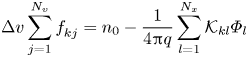
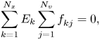
We consider the Vlasov–Poisson system on a two-dimensional phase space for a mobile species of charge $q$ and mass $m$
 . For simplicity we assume a static, uniform, neutralizing background with density $n_0$
 . The distribution function, $f$
 , for the mobile species then satisfies
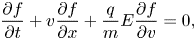
where $E=-\partial \varPhi / \partial x$ is the electric field and $\varPhi$
 the potential, which is determined through Poisson's equation,

We assume the spatial domain is periodic and take the average value of $\varPhi$ to be zero and assume $f\rightarrow 0$
 as $|v|\rightarrow \infty$
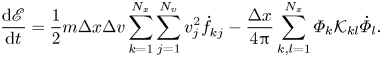
 . The energy of the system is given by

where we have integrated by parts in the last term. It is well known that this system possesses an infinity of Casimir invariants of the form $\int \!{{\rm d}x}\,{{\rm d}}v\,C(f)$ , for any function $C$
 .
.
2. Phase-space discretization
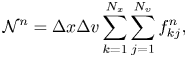
Here we consider a purely Eulerian numerical solution of (1.1), that is, we will solve (1.1) on a phase-space grid without recourse to characteristics. We construct a regular, uniform grid of points $(x_k, v_j)$ over phase space of size ${{N_x}}\times {{N_v}}$
 with $x_k = x_1 + (k-1){{\Delta x}}$
 , $k=1,\ldots,{{N_x}}$
 where ${{\Delta x}} = (x_{{N_x}} - x_1)/({{N_x}}-1)$
 and $v_j = v_1 + (j-1){{\Delta v}}$
 , $j=1,\ldots,{{N_v}}$
 where ${{\Delta v}} = (v_{{N_v}} - v_1)/({{N_v}}-1)$
 . Periodicity in $x$
 is imposed by identifying $x_{{N_x}} + {{\Delta x}}$
 with $x_1$
 and consequently $x_1 - {{\Delta x}}$
 with $x_{{N_x}}$
 . The periodicity length, $L$
 , of the spatial domain is then $L = x_{{N_x}} + {{\Delta x}} - x_1$
 and ${{\Delta x}} = L/{{N_x}}$
 . The velocity grid is assumed to contain the support of $f$
 , thus we take $f(x, v_1-{{\Delta v}}, t) = 0 = f(x, v_{{N_v}}+{{\Delta v}}, t)$
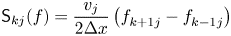
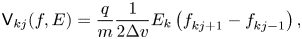
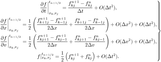
 . We first consider discretizing phase space while leaving time continuous. Approximating the phase-space derivatives by second-order central difference expressions, we have

and

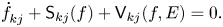
where ${f}^{}_{{k}{j}}(t)$ is the numerical approximation to $f(x_k, v_j, t)$
 , the dot signifies differentiation with respect to $t$
 , $E_k = (\varPhi _{k-1} - \varPhi _{k+1})/(2{{\Delta x}})$
 , $\varPhi _k$
 is the numerical approximation to $\varPhi (x_k)$
 and
and
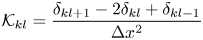
is a second-order accurate approximation to second spatial derivative. To keep the subsequent algebra manageable, it is convenient to define
and
which allows us to write (2.1a) as
This discretization has also been applied to the relativistic Vlasov–Maxwell system (Shiroto, Ohnishi & Sentoku Reference Shiroto, Ohnishi and Sentoku2019).
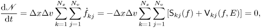
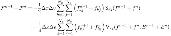
All of the invariants of (1.1) will have analogues in (2.1), consistent with the second-order accuracy of the phase-space discretization, that is, although time remains continuous, we cannot expect invariants of (2.1) to be constant beyond $O(\Delta x^{2}) + O(\Delta v^{2})$ . There are four invariants that survive phase-space discretization: particle number,

momentum,
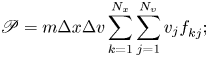
energy,
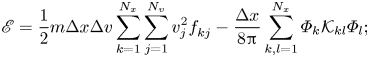
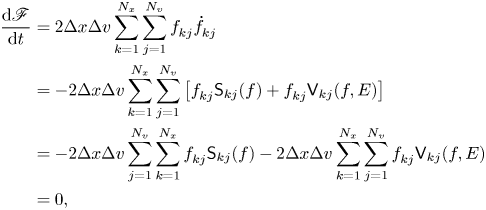
and enstrophy

Armed with a collection of identities, (A2)–(A13), demonstrating the invariance of these quantities is relatively straightforward. Consider
where the last step follows from (A2) and (A7) and the assumption that the computational domain is large enough that no particle flux reaches the boundary of the velocity domain. Now

where we have used (A2) and (A9) and we have assumed no momentum flux reaches the boundary of the velocity domain. From Poisson's equation, we have
and

where we have used (2.2). Since our spatial domain is periodic, we can interpret spatial indices modulo ${{N_x}}$ ; shifting the spatial index in sums has no effect. Thus $\sum _{k=1}^{N_x}\varPhi _{k+1}=\sum _{k=1}^{N_x}\varPhi _{k-1} = 0$
 due to our normalization of $\varPhi$
 and $\sum _{k=1}^{N_x}\tilde {\varPhi }_{k+1}^{2} = \sum _{k=1}^{N_x}\tilde {\varPhi }_{k-1}^{2}$
 , and $\sum _{k=1}^{N_x}\tilde {\varPhi }_k\tilde {\varPhi }_{k+1} = \sum _{k=1}^{N_x}\tilde {\varPhi }_{k-1}\tilde {\varPhi }_k$
 , giving
which then implies $d\mathscr {P}/dt = 0$ . Now
. Now
From (2.1a′), we have

where the last step follows from (A2) and (A11) and the assumption that the particle energy flux vanishes at the velocity boundaries. From (2.1a′), (2.1b) and (A7) we have

giving

where (A5) has been used. Combining (2.16) and (2.17), we see $d\mathscr {E}/dt = 0$ . Lastly,
where we have used (A4) and (A13). From the reasoning that leads to (A4) and (A13), it is easy to see that for Casimirs involving higher powers of ${f}^{}_{{k}{j}}$ cancellations, analogous to those leading to (2.18) will not occur. Thus particle number and enstrophy are the only Casimirs to survive on a phase-space grid. While we have considered a spatially periodic system, in an unbounded domain, assuming the distribution function vanishes for large $|x|$
 , these conservation laws continue to hold (in both the continuum and discrete cases). In a bounded but not periodic system, the validity of the conservation laws will depend on the details of the spatial boundary conditions. These results all generalize straightforwardly to higher-order centred differences approximations for the derivatives in in $\mathsf {S}_{kj}$
 and $\mathsf {V} _{kj}$
 .
.
3. Time integration
To obtain a numerical solution of (2.1) requires the introduction of a discrete time step. The time integration runs from ${t_{I}}$ to ${t_{F}}$
 with fixed time step ${{\Delta t}}$
 and ${{N_t}}$
 steps, giving ${{\Delta t}} = ({t_{F}} - {t_{I}})/{{N_t}}$
 . We put $t_n = t_1 + (n-1){{\Delta t}}$
 , thus $t_1 = {t_{I}}$
 and ${t_{F}} = t_{{{N_t}}}$
 . Without loss of generality, we may assume $t_1 = 0$
 . In what follows, we take ${f}^{n}_{{k}{j}}$
 to be the numerical approximation of $f(x_k, v_j, t_n)$
 . We consider two related temporal discretizations: (i) the midpoint rule; and (ii) the midpoint rule combined with operator splitting.
First consider discretizing (2.1) at ${{t_{n+1/2}}}$ :
:

where $E^{n}_k = (\varPhi ^{n}_{k-1} - \varPhi ^{n}_{k+1})/2{{\Delta x}}$ ,
,

Using the linearity of $\mathsf {S}_{kj}$ and $\mathsf {V} _{kj}$
 , we can write (3.1a) as
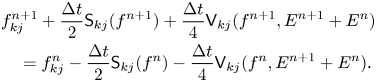
There are other possible discretizations of the nonlinear term in (2.1a); this particular choice is attractive because, as we will see below, it leads to exact energy conservation.Footnote 1 This discretization is equivalent to applying the Crank–Nicolson time-centred scheme (Crank & Nicolson Reference Crank and Nicolson1947) to (1.1) (see figure 1):
Together, (3.1a) and (3.1b) define a nonlinear systems of equations that, given ${f}^{n}_{{k}{j}}$ , must be solved for ${f}^{n+1}_{{k}{j}}$
 . This system is large – ${{N_x}}\times {{N_v}}$
 unknowns – and sparse but with considerable bandwidth, thus any direct solution is impractical. The now-standard approach to such problems are Jacobian-free Newton–Krylov methods (Knoll & Keyes Reference Knoll and Keyes2004); while effective, these methods can be computationally intensive. The advantage of this temporal discretization is that all of the invariants that survive phase-space discretization, (2.5)–(2.8), are also invariants of the resulting time advance.
The Crank–Nicolson stencil for the Vlasov equation.

We define discrete-time analogues of $\mathscr {N}$ , $\mathscr {P}$
 , $\mathscr {E}$
 and $\mathscr {F}$
 in the obvious way:


and

From (3.2), (A2) and (A7) we readily see $\mathcal {N}^{n+1} = \mathcal {N}^{n}$ . Using (3.1a) and (A2), we find

where we have used (A9) in the last step. From the linearity of Poisson's equation, $(E^{n+1} + E^{n})/2$ is the field due to the phase-space density $(f^{n+1} + f^{n})/2$
 , and thus by same reasoning that leads to (2.13), we have

and thus $\mathcal {P}^{n+1} = \mathcal {P}^{n}$ . A direct consequence of momentum conservation is that this algorithm is free of self-forces. Now from (3.1a) and (A2), we have
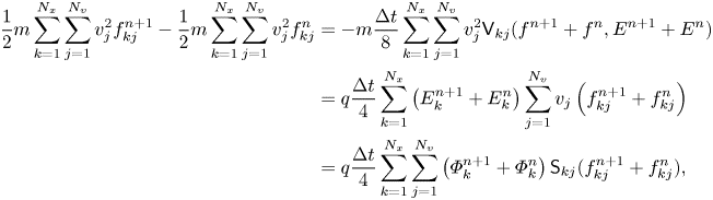
where we have used (A5) in the last step. From (3.1a) and (A7) we see

and thus

giving

From (3.1b), we have

and hence

Since we normalize $\varPhi _k$ to have zero average value, this becomes
The right-hand side of (3.16) is symmetric under $m \leftrightarrow n$ and we can conclude
and thus

Combining (3.18) and (3.13), we have

which is equivalent to $\mathcal {E}^{n+1} = \mathcal {E}^{n}$ . Finally, consider

Using (3.1a), we can write this as
which, in view of (A4) and (A13), leads to $\mathcal {F}^{{n+1}} = \mathcal {F}^{ {n}}$ . The invariance of $\mathcal {F}^{ {n}}$
 precludes numerical solutions with strict exponential growth in time, thus the time advance is unconditionally stable (Schumer & Holloway Reference Schumer and Holloway1998). These quantities are also conserved by methods employing a Hermite basis in velocity (Schumer & Holloway Reference Schumer and Holloway1998; Bourdiec, de Vuyst & Jacquet Reference Bourdiec, de Vuyst and Jacquet2006; Delzanno Reference Delzanno2015; Camporeale et al. Reference Camporeale, Delzanno, Bergen and Moulton2016).
We now consider an integration algorithm where we split the discretized Vlasov equation (2.1a′) into two advection operators

and

which has the effect of removing the nonlinearity and removing one independent variable at each operator; in (3.22a) $v_j$ acts as a parameter, while in (3.22b) $x_k$
 is parametric. Although $E$
 is dependent on $f$
 , the charge density, and thus the electric field, is invariant under the action of (3.22b), and thus (3.22b) is effectively linear in $f$
 . This is the same splitting used by Cheng & Knorr (Reference Cheng and Knorr1976) in their semi-Lagrangian method, by Schumer & Holloway (Reference Schumer and Holloway1998) in their Hermite spectral algorithm and by Sircombe & Arber (Reference Sircombe and Arber2009) in constructing explicit Eulerian methods. To second-order accuracy in time, we can compute the time evolution of (2.1) using the symmetric Strang approach (Strang Reference Strang1968) as illustrated in figure 2. Let the operators $U_1(t,{{\Delta t}})$
 and $U_2(t,{{\Delta t}})$
 give the evolution of $f$
 from $t$
 to $t + {{\Delta t}}$
 corresponding to (3.22a) and (3.22b), respectively. Provided the $U_i$
 are at least second-order accurate in ${{\Delta t}}$
 (or first-order accurate and time reversible (Kahan & Li Reference Kahan and Li1997)), the evolution corresponding to (2.1) from $t$
 to $t +{{\Delta t}}$
 is given by

and is accurate to second order in ${{\Delta t}}$ .
.


Following this prescription and using Crank–Nicholson discretization for (3.22a) and (3.22b), we arrive at the following set of equations describing the evolution of the distribution function:


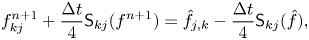
where $\tilde {E}_k = (\tilde {\varPhi }_{k-1} - \tilde {\varPhi }_{k+1})/(2{{\Delta x}})$ and
and

Thus, given ${f}^{n}_{{k}{j}}$ , we solve (3.24a) to obtain ${\tilde {f}}^{}_{{k}{j}}$
 and subsequently $\tilde {\varPhi }$
 through (3.24d). We then solve (3.24b) to obtain ${\hat {f}}^{}_{{k}{j}}$
 and finally solving (3.24c) yields ${f}^{n+1}_{{k}{j}}$
 . Not only are all of these equations linear in the unknowns, the linear systems are tridiagonal and thus amenable to efficient direct solution. In all cases we use the Thomas algorithm (Thomas Reference Thomas1949) to solve the linear systems, and handle the periodic boundary conditions through the Sherman–Morrison formula (Hager Reference Hager1989). Thus even though the discretization is implicit in time, reducing the number of independent variables results in low-bandwidth linear systems.
Since (3.24) is a consistent approximation to (2.1), all invariants of (2.1) will be approximately conserved to at least $O(\Delta t^{2})$ . It turns out that $\mathcal {N}$
 , $\mathcal {P}$
 and $\mathcal {F}$
 are exactly conserved by (3.24) while energy is only approximately conserved.

and likewise from (3.24c)

Together these imply $\mathcal {N}^{n+1} = \mathcal {N}^{n}$ . From (A2) and (3.24a) and (3.24c), we have, for all $j$
 ,
,

and

respectively. From (3.24b) and (A9) we have
Using (3.27) we can write

where the last step follows from the same reasoning that leads to (2.13). Thus we have

and hence, with (3.28) and (3.29), $\mathcal {P}^{n+1} = \mathcal {P}^{n}$ . Now, using (3.24a) and (A4), we have
and likewise
Finally, from (3.24b) and (A13), we have
Thus we have
and $\mathcal {F}^{ {n+1}} = \mathcal {F}^{ {n}}$ . Again, invariance of $\mathcal {F}$
 implies unconditional stability of the algorithm (Schumer & Holloway Reference Schumer and Holloway1998).
4. Benchmarking
Here we consider a variety of test cases that have been used extensively in the literature (Zaki, Boyd & Gardner Reference Zaki, Boyd and Gardner1988; Filbet & Sonnendrücker Reference Filbet and Sonnendrücker2003; Shoucri Reference Shoucri2008; Heath et al. Reference Heath, Gamba, Morrison and Michler2012) where the numerical results can be compared with analytical solutions or growth rates. Unless specified otherwise, we use an initial distribution function of the form

with

where ${v_\mathrm {th}}$ is the thermal velocity, $k$
 and $A$
 are the wavenumber and amplitude of the initial disturbance, respectively. When considering the linearized theory, we split the initial condition into $f_0 = f_0^{(0)} + f_0^{(1)}$
 with
with

Periodic boundary conditions in space require the wavenumber to be quantized as $k=2{\rm \pi} l/L$ , with $l$
 an integer. We take $L = 4{\rm \pi} \lambda _D$
 , where $\lambda _D = {v_\mathrm {th}}/\omega _p$
 is the Debye length and $\omega _p = \sqrt {4{\rm \pi} n_0q^{2}/m}$
 is the plasma frequency, and thus allowable values of $k$
 are given by ${k\lambda _D} = l/2$
 .
.
4.1. Ballistic Motion
We consider the ballistic transport of uncharged particles corresponding to

Since the distribution function must remain constant along characteristics, the evolution of the particle density can be calculated analytically

which we can integrate to give

We solve (4.5) using our split algorithm simply skipping (3.24b); since $E=0$ , (3.24b) reduces to ${\hat {f}}^{}_{{k}{j}} = {\tilde {f}}^{}_{{k}{j}}$
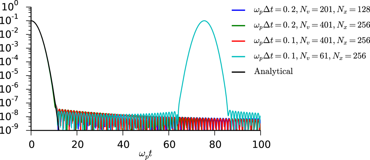
 . In figure 3 we plot the maximum of the particle density as a function of time for $A=0.1$
 , ${k\lambda _D}=1/2$
 , $\omega _p{t_{F}} = 100$
 , and various values of $\omega _p{{\Delta t}}$
 , ${{N_v}}$
 and ${{N_x}}$
 on the velocity domain $[-5{v_\mathrm {th}}, 5{v_\mathrm {th}}]$
 . The numerical and analytical results are in excellent agreement early in the simulation. The density reaches a plateau due to the periodic boundary conditions before returning to its original state with the recurrence time defined by ${t_{R}} = 2{\rm \pi} /k{{\Delta v}}$
 (Cheng & Knorr Reference Cheng and Knorr1976). Using the definition of $\lambda _D$
 , we can write $\omega _p{t_{R}} = (2{\rm \pi} /{k\lambda _D})({v_\mathrm {th}}/{{\Delta v}})$
 . For our parameters, only the coarsest velocity grid (${{N_v}} = 61$
 ) yields a recurrence time less than ${t_{F}}$
 : $\omega _p{t_{R}} = 24{\rm \pi} \approx 75.4$
 . The second peak in figure 3 occurs at $\omega _p t = 75.50$
 in excellent agreement with this estimate.
Evolution of the maximum particle density, normalized to $n_0$ , for $A=0.1$
 , ${k\lambda _D}=1/2$
 and various grid parameters. The black line corresponds to (4.7).
4.2. Linear Landau damping
Linear Landau damping provides a sensitive test of phase-space dynamics due to the central role of phase mixing in the damping phenomena and is a convenient benchmark as the damping rate can be readily calculated. To avoid having nonlinear effects pollute our numerical result, we solve the linearized Vlasov equation (see Appendix B for details). We set $A=0.1$ and ${k\lambda _D} = 1/2$
 , resulting in a single weakly damped mode and take the velocity domain to be $[-8{v_\mathrm {th}}, 8{v_\mathrm {th}}]$
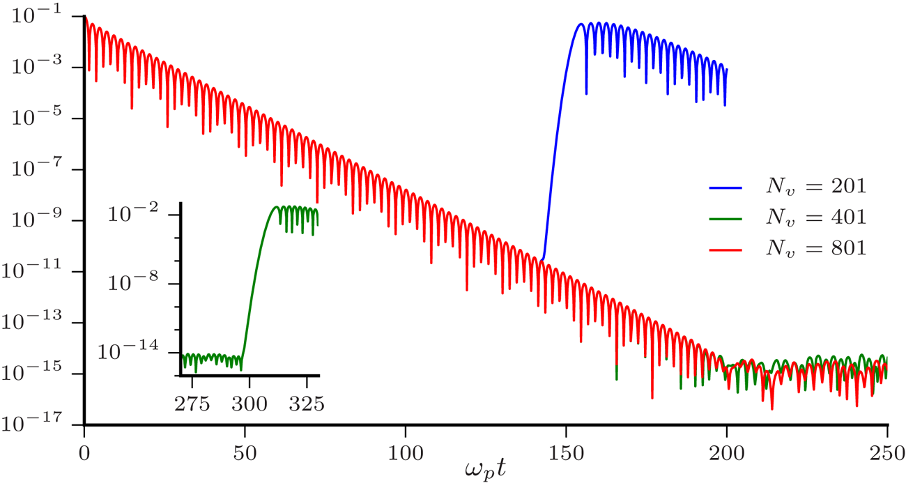
 . In figure 4 we plot the evolution magnitude of the dominant ($l = 1$
 ) spatial Fourier mode of electric field. The decay of the fundamental mode is sustained over many decades until either a recurrence occurs or the limit of numerical precision in computing the perturbed charge density is reached. As in Cheng & Knorr (Reference Cheng and Knorr1976), the recurrences seen in figure 4 agree with the ballistic estimates $\omega _p{t_{R}} = 50{\rm \pi} \approx 157.1$
 for ${{N_v}} = 201$
 and $\omega _p{t_{R}} = 100{\rm \pi} \approx 314.2$
 for ${{N_v}} = 401$
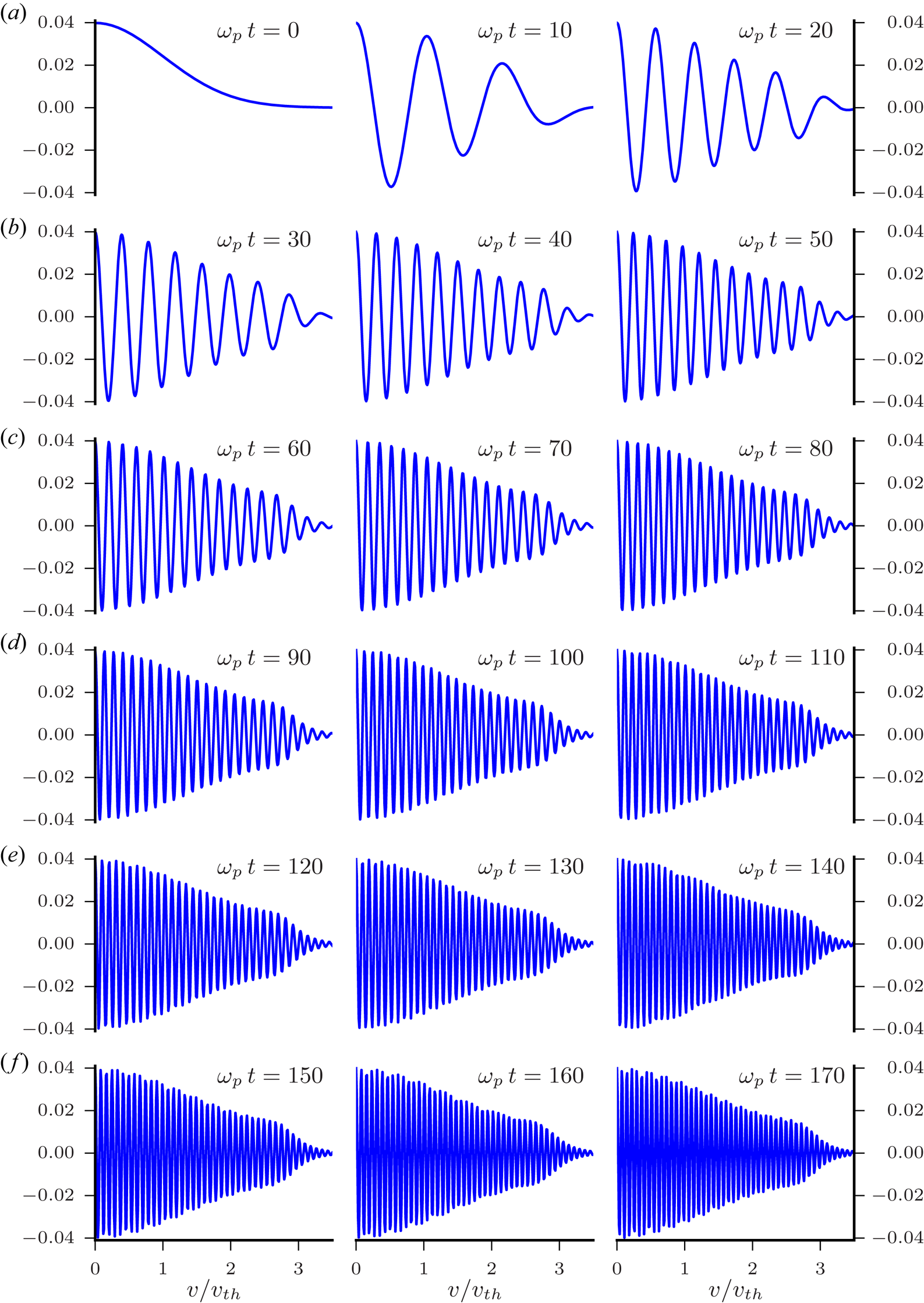
 . Shown in figure 5 is the evolution of perturbed distribution function at $x=0$
 with ${{N_v}}=1601$
 . The effects of filamentation are clearly evident.
Magnitude of the spatial Fourier component of the electric field corresponding to ${k\lambda _D} = 1/2$ with $\omega _p{{\Delta t}} = 0.1$
 and ${{N_x}} = 256$
 and various values of ${{N_v}}$
 , normalized to $\omega _p m{v_\mathrm {th}}/q$
 . The inset shows the recurrence for ${{N_v}} = 401$
 .
.
Time evolution of the perturbed distribution function, normalized to $n_0/{v_\mathrm {th}}$ , for the parameters of figure 4 and ${{N_v}}=1601$
 at $x = 0$
 . The vertical and horizontal scales are the same for all panels.
In the linearized case, the perturbations to the particle number and momentum are exactly conserved in discrete time; the proof is essentially the same as in the nonlinear case. Our numerical results yield conservation of these quantities to within a small multiple of machine precision. Additionally, the Kruskal–Oberman energy, (B3), is an exact invariant (Kruskal & Oberman Reference Kruskal and Oberman1958; Morrison & Pfirsch Reference Morrison and Pfirsch1990). The discrete analogue of (B3) is

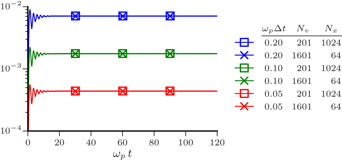
As discussed in Appendix B, the error in this invariant is due to temporal discretization alone. Shown in figure 6 is the absolute value of the relative error in $\mathcal {E}_\mathrm {KO}$ ; clearly the overall scale of the error is dependent only on $\omega _p{{\Delta t}}$
 . It seems plausible that an exactly conservative (Shadwick, Bowman & Morrison Reference Shadwick, Bowman and Morrison1999) time integration scheme could be developed; this will be explored in a future publication. van Kampen constructed an exact solution to the linearized Vlasov equation using singular eigenfunctions (van Kampen Reference van Kampen1955; van Kampen & Felderhof Reference van Kampen and Felderhof1967). One particularly interesting aspect of this construction is that it allows for the electric field to be written in terms of the initial distribution and various equilibrium quantities. Following van Kampen & Felderhof (Reference van Kampen and Felderhof1967) and using the notation of Shadwick (Reference Shadwick1995) we can write the spatial Fourier transform of the electric field as

where $\epsilon _r$ and $\epsilon _i$
 are, respectively, the real and imaginary parts of the plasma dielectric function corresponding to the equilibrium, (B13), (in the limit $\omega _I \rightarrow 0^{+}$
 ; see Appendix B), $F_k(v)$
 is the spatial Fourier transform of $f_0^{(1)}$
 and the overbar indicates the Hilbert transform (Tricomi Reference Tricomi1985). Here
and

where $\operatorname {daw}(x)$ is Dawson's integral (Abramowitz & Stegun Reference Abramowitz and Stegun1964). Both ${f_{\textrm {eq}}}$
 and $\epsilon _r$
 are even functions while $\overline {{f_{\textrm {eq}}}}$
 and $\epsilon _i$
 are odd functions, allowing us to write

Normalizing the electric field to $\omega _p m{v_\mathrm {th}}/q$ , we have

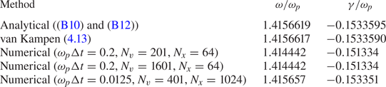
We compute $\mathbb {E}_k$ directly from (4.13) with SciPy (Jones, Oliphant & Peterson Reference Jones, Oliphant and Peterson2001) using adaptive quadrature. In figure 7(a) we show a comparison between the van Kampen solution, (4.13), blue line, the finite-difference solution with $\omega _p{{\Delta t}} = 0.025$
 , ${{N_x}} = 512$
 , and ${{N_v}} = 401$
 , dashed red line, and a fit to a damped oscillation (see below), dashed black line. As can be seen from the inset, while a fixed frequency and damping rate does not describe the behaviour at early time, the finite difference and van Kampen solutions are in close agreement for all $t$
 . Figure 7(b) shows the absolute value of the relative error between the finite difference and van Kampen solutions evaluated at the local maxima of $|\mathbb {E}_k|$
 for $\omega _p {{\Delta t}} = 0.025$
 , ${{N_x}} = 512$
 , ${{N_v}} = 401$
 (black squares) and $\omega _p\,{{\Delta t}} = 0.0125$
 , ${{N_x}} = 1024$
 , ${{N_v}} = 401$
 (red circles). Reducing ${{\Delta t}}$
 and ${{\Delta x}}$
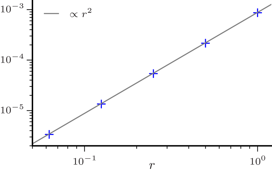
 by a factor of two results in a reduction in the error by an amount consistent with the expected second-order accuracy of the scheme. Figure 8 shows the $L^{2}$
 norm of the difference between the van Kampen and finite-difference solutions with $\omega _p{{\Delta t}} = 0.2r$
 and ${{N_x}} = 64/r$
 for $1/16 \le r \le 1$
 . The reduction in the $L^{2}$
 norm with $r$
 is consistent with the second-order accuracy of the discretization.
Absolute value of the relative error in the Kruskal–Oberman energy, (4.8), for various grid parameters. As can be seen, the energy error only depends on the temporal discretization.
Comparison of the spatial Fourier transform of the electric field from the finite difference and van Kampen solutions: (a) the van Kampen solution, (4.13) (blue line), the finite-difference solution with $\omega _p{{\Delta t}} = 0.025$ , ${{N_x}} = 512$
 and ${{N_v}} = 401$
 (dashed red line), and a fit to a damped oscillation (see text) (dashed black line), normalized to $\omega _p m{v_\mathrm {th}}/q$
 ; (b) the absolute value of the relative error between the finite difference and van Kampen solutions evaluated at the local maxima of $|\mathbb {E}_k|$
 for $\omega _p{{\Delta t}} = 0.025$
 , ${{N_x}} = 512$
 , ${{N_v}} = 401$
 (black squares) and $\omega _p{{\Delta t}} = 0.0125$
 , ${{N_x}} = 1024$
 , ${{N_v}} = 401$
 (red circles). The inset shows that the solutions agree at early time but are not well-reproduced by a damped oscillation.

The $L^{2}$ norm of the difference of the spatial Fourier transform of the electric field, normalized to $\omega _p m{v_\mathrm {th}}/q$
 , from the finite difference and van Kampen solutions with $\omega _p{{\Delta t}} = 0.2r$
 , ${{N_x}} = 64/r$
 and ${{N_v}} = 401$
 (crosses). The results show no meaningful variation with ${{N_v}}$
 .
.
To determine the frequency and damping rate, we fit the Fourier transform of the electric field to
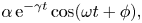
over the range $\omega _p t=10$ to $\omega _p t=180$
 . (For ${{N_v}} = 201$
 , we stop the fit at $\omega _p t = 120$
 due to the recurrence.) The results of this fitting along with the analytical values are summarized in table 1. As can be seen, the analytical results and the fit to the van Kampen solution are in very good agreement. Both of these results are consistent with previous results (Cheng & Knorr Reference Cheng and Knorr1976; Filbet, Sonnendrücker & Bertrand Reference Filbet, Sonnendrücker and Bertrand2001; Heath et al. Reference Heath, Gamba, Morrison and Michler2012). Evaluating the van Kampen solution using (4.13) involves highly oscillatory integrands; a specialized method was not employed and so it is reasonable to assume the minor difference between the analytical values and the fit to the van Kampen solution is not meaningful. The frequency and damping rate inferred from the finite-difference solution agrees quite well with the van Kampen solution and this agreement improves as the resolution is increases. Note, for our parameters the frequency and damping rate are remarkably insensitive to ${{\Delta v}}$
 . Figure 9 shows the absolute value of the relative error between the analytical frequency (a, b) and damping rate (c, d) the corresponding values obtained by fitting the finite difference solution to (4.14). As is to be expected, it is necessary to refine both ${{\Delta t}}$
 and ${{\Delta x}}$
 to improve the accuracy of the solution. We see that the accuracy of the finite-difference solution is second order in both ${{\Delta t}}$
 and ${{\Delta x}}$
 . The plot is identical if instead we compare with the frequency and damping rate obtained from the van Kampen solution.
Relative error in the frequency (a,b) and damping rate (c,d) for various value of ${{\Delta t}}$ and ${{\Delta x}}$
 with ${{N_v}} = 401$
 . The results show no meaningful variation with ${{N_v}}$
 .
.

Summary of fitting the magnitude of the Fourier transform of the electric field to (4.14).
For weak Landau damping with somewhat different parameters we have compared the full nonlinear solver with a variational macroparticle model using both standard and symplectic integration and found excellent agreement (Shadwick et al. Reference Shadwick, Stamm and Evstatiev2014). In that case the limit of the comparison was the inability of the macroparticle model to continue to exhibit damping once the charge density reached the level comparable to that associated with the fluctuations inherent in representing the initial Maxwellian distribution.
4.3. Nonlinear Landau damping
We now consider the full nonlinear response with $A = 0.5$ , ${k\lambda _D} = 1/2$
 , spatial domain $[0, 4{\rm \pi} \lambda _D]$
 and velocity domain $[-10{v_\mathrm {th}}, 10{v_\mathrm {th}}]$
 . Figure 10 shows the amplitude of the spatial Fourier transform of the electric field corresponding to ${k\lambda _D} = 1/2$
 , 1 and $3/2$
 . As a consequence of the nonlinear coupling, energy is transferred from the fundamental mode resulting in a damping rate that well exceeds the value in the linear case. We find $\gamma \approx -0.283\omega _p$
 for the initial decay and $\gamma \approx 0.081\omega _p$
 for the subsequent growth which is in good agreement with previous results (Cheng & Knorr Reference Cheng and Knorr1976; Zaki et al. Reference Zaki, Boyd and Gardner1988; Filbet et al. Reference Filbet, Sonnendrücker and Bertrand2001; Heath et al. Reference Heath, Gamba, Morrison and Michler2012). Figure 11 shows the evolution of the spatial average of the distribution function; since $f$
 is symmetric in $v$
 , only $v \ge 0$
 is shown. These results are in quantitative agreement with some previous results (Cheng & Knorr Reference Cheng and Knorr1976; Zaki et al. Reference Zaki, Boyd and Gardner1988) but differ somewhat with Heath et al. (Reference Heath, Gamba, Morrison and Michler2012), which seems to be related to the dissipation in their algorithm.
Amplitude of the spatial Fourier modes of the electric field, normalized to $\omega _p m{v_\mathrm {th}}/q$ , for $\omega _p{{\Delta t}} = 0.05$
 , ${{N_v}} =1001$
 and ${{N_x}} = 1024$
 .
.

Time evolution of the spatial average of the distribution function, normalized to $n_0/{v_\mathrm {th}}$ , for nonlinear Landau damping with the parameters of figure 10. The vertical and horizontal scales are the same for all panels.
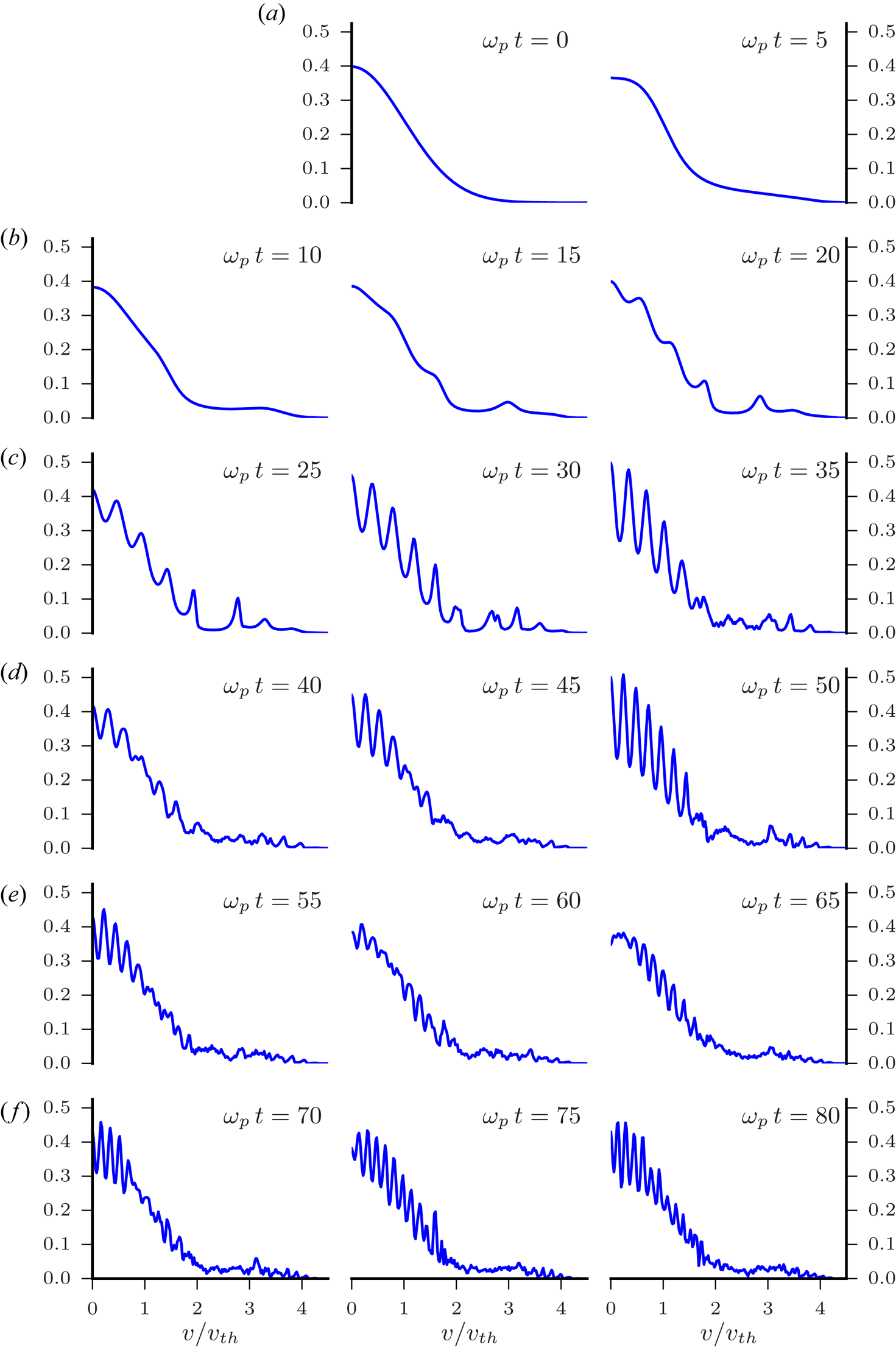
Figure 12 shows the absolute value of the relative error in energy, $\mathcal {E}$ , (a); relative error in particle number, $\mathcal {N}$
 , and enstrophy, $\mathcal {F}$
 , (b, c), respectively; and error in momentum, $\mathcal {P}$
 , (d) for different grid parameters. As in the linear case, the energy error depends only on ${{\Delta t}}$
 which follows from $\mathscr {E}$
 being an exact invariant of the continuous-time system (2.1). Particle number, enstrophy and moment are exact invariants of the algorithm but exhibit variation well beyond typical rounding levels even with using extended precision to calculate these quantities. Furthermore, their variation does not appear to depend systematically on the grid parameters. The behaviour of these quantities turns out to be extremely sensitive to the numerical parameters. Shown in figure 13 are $\mathcal {N}$
 , $\mathcal {F}$
 and $\mathcal {P}$
 for $\omega _p{{\Delta t}} = 0.1$
 and various values of ${{N_x}}$
 and ${{N_v}}$
 . The curves with the solid symbols correspond to a spatial domain size of $L = 12.566370614359172\lambda _D$
 , while the curves with the open symbols correspond to $L = 12.5663706144\lambda _D$
 . The difference in the domain size between the two cases is approximately three parts in $10^{12}$
 , yet the behaviour of the invariants is markedly different. Preservation of the invariants relies on the linear systems in each step of (3.24) being solved exactly, that is, to machine precision. While we are using direct solution of the linear systems (the Thomas algorithm (Thomas Reference Thomas1949)), we still expect a non-vanishing residual from each step. It seems reasonable to conclude that the behaviour seen in figure 13 is due to the well known numerical sensitivity of direct linear solvers. It may be possible that by using iterative refinement (Moler Reference Moler1967) of the solution at each step, the invariants could be maintained close to machine precision.
Invariant preservation in nonlinear Landau damping: absolute relative error in particle number, $\mathcal {N}$ , total energy, $\mathcal {E}$
 , enstrophy, $\mathcal {F}$
 , (a–c), respectively; and error in momentum, $\mathcal {P}$
 , normalized to $mn_0{v_\mathrm {th}}$
 , (d) for different grid parameters.
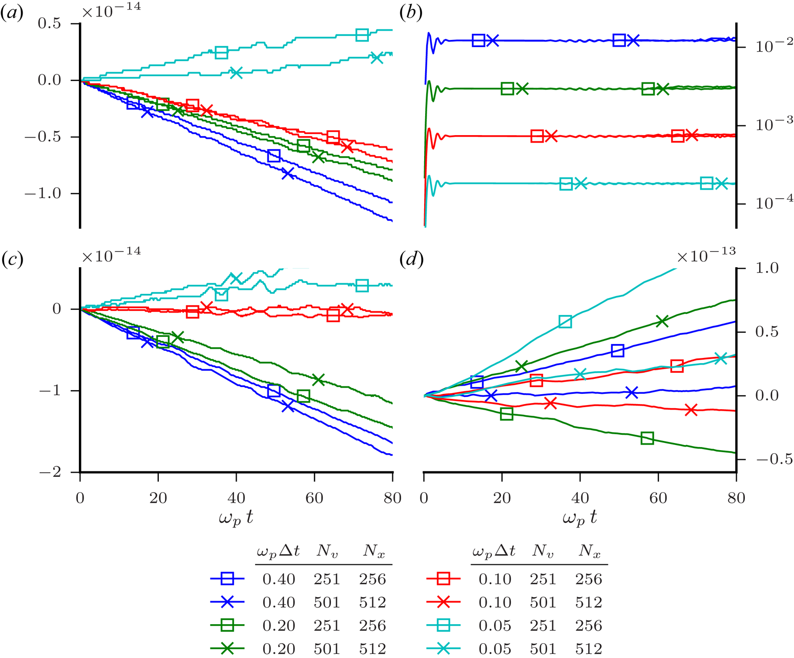
Invariant preservation in nonlinear Landau damping: relative error in particle number, $\mathcal {N}$ , and enstrophy, $\mathcal {F}$
 , (a,b), respectively; and error in momentum, $\mathcal {P}$
 , normalized to $mn_0{v_\mathrm {th}}$
 , (c) for $\omega _p{{\Delta t}} = 0.1$
 and various values of ${{N_x}}$
 and ${{N_v}}$
 . Solid symbols correspond to a spatial domain size of $L = 12.566370614359172\lambda _D$
 , while open symbols correspond to $L = 12.5663706144\lambda _D$
 .
.

4.4. Two-stream instability
We now consider the two-stream instability with the equilibrium distribution function (Cheng & Knorr Reference Cheng and Knorr1976)

which mimics two counter-propagating electron beams. For this distribution ${v_\mathrm {th}} = \sqrt {3}v_0$ and $\lambda _D = \sqrt {3}v_0/\omega _p$
 . To aid comparison with the existing literature we take, in contrast to previous sections, $v_0$
 and ${{\bar {\lambda }}} = v_0/\omega _p = \lambda _D/\sqrt {3}$
 as our velocity and length scales, respectively. We use the initial condition (4.1) with $A = 10^{-6}$
 , ${k{\bar {\lambda }}} = 1/2$
 with $L = 4{\rm \pi} {{\bar {\lambda }}}$
 and velocity domain $[-10v_0, 10v_0]$
 . Our parameters allow for only a single linearly unstable mode (see Appendix B). Figure 14 shows the magnitude of the first four spatial Fourier modes of the electric field. After some initial Landau damping the unstable mode emerges. The initial behaviour of the $l = 1$
 mode is in good agreement with the linear theory (dashed purple line) as can been seen from the inset which absolute value of the relative difference between the linear and nonlinear solutions for $l = 1$
 . Since only the $l = 1$
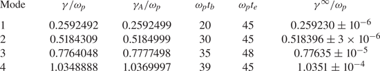
 mode is linearly unstable, the higher modes seen in figure 14 grow due to nonlinear coupling. Table 2 shows the growth rates for modes 1–4. The logarithm of magnitude of Fourier transform of electric field was fitted to $\alpha + \gamma t$
 over the interval $[t_b, t_e]$
 . To study convergence, we scale $\omega _p{{\Delta t}} \propto r$
 and ${{N_x}}$
 and ${{N_v}} \propto 1/r$
 ; specifically we take $\omega _p{{\Delta t}} = 0.125r$
 , ${{N_x}} = 128/r$
 and ${{N_v}} = 125/r$
 with $r = 1$
 , $1/2$
 , $1/4$
 , $1/8$
 and $1/16$
 . For the four modes considered, we observe nearly perfect second-order convergence of the growth rates with increasing resolution (decreasing $r$
 ) but to values that differ somewhat from the predictions of linear theory. We can exploit the observed convergence to extrapolate to infinite resolution ($r = 0$
 ) by fitting the results to $\gamma = \gamma ^{\infty } + \delta r^{2}$
 where $\gamma ^{\infty }$
 is then the estimate of the growth rate in the limit ${{\Delta t}}, {{\Delta x}}, {{\Delta v}} \rightarrow 0$
 . The result of this extrapolation is given in table 2 in the column labelled $\gamma ^{\infty }/\omega _p$
 together with error estimates derived from the fit covariance.
Magnitude of the spatial Fourier modes of the electric field, normalized to $m\omega _p v_0/q$ , for the two-stream problem with $\omega _p{{\Delta t}} = 0.0625$
 , ${{N_v}} = 2001$
 and ${{N_x}} = 2048$
 and initial conditions (4.1) and (4.15). The fundamental mode corresponds to ${k{\bar {\lambda }}} = 1/2$
 . The dashed purple line shows the magnitude of the electric field obtained from the linearized equations for the same numerical parameters and initial condition. The inset shows the absolute value of the relative difference between the linear and nonlinear results for $n = 1$
 .
.

Growth rates, $\gamma$ , for the two-stream instability and analytical values obtained from perturbation theory, $\gamma _A$
 , for the parameters of figure 14. The wavenumber for mode $n$
 is given by ${k{\bar {\lambda }}} = n/2$
 . For each mode the fit was performed over $[t_b, t_e]$
 .
.
In figure 15 we plot the absolute value of the relative error in energy, $\mathcal {E}$ , (a); relative error in particle number, $\mathcal {N}$
 , and enstrophy, $\mathcal {F}$
 , (b,c), respectively; and error in momentum, $\mathcal {P}$
 , (d) for the parameters of figure 14. In figure 16 we plot the distribution function over the interesting region of phase space for selected values of $t$
 . The distribution function evolves in the expected way through approximately $\omega _p t = 60$
 . It is well known that the lack of dissipation when using Crank–Nicolson discretization can cause the numerical solution to overshoot and undershoot in regions of steep gradients (essentially a Gibbs-like phenomena). By $\omega _p t = 65$
 (and indeed earlier; see below), the distribution function begins to exhibit negative values. Since $\mathcal {N}$
 is conserved, there must be regions that are ‘excessively’ positive to compensate. Empirically, the charge density appears to be largely unaffected by these unphysical values and thus the electric field appears to remain reliable. The invariance properties of the algorithm are not dependent on maintaining $f \ge 0$
 and thus the structure of phase space away from these regions should be rendered faithfully. As one would expect, these negative values follow the evolution of the $v = 0$
 trough in the initial condition. This is evident in figure 17 where we plot the phase-space locations where $f < 0$
 . The topological conservation properties discussed in Heath et al. (Reference Heath, Gamba, Morrison and Michler2012) are clearly violated by this behaviour. In addition to being obviously unphysical, negative values of $f$
 are inconsistent with the rearrangement dynamics of the Vlasov equation Gardner (Reference Gardner1963). Furthermore, adjacent to the grid points where $f < 0$
 are grid points where $f$
 is erroneously large. As a result the global maximum of $f$
 exceeds the maxima in the initial condition at $v = \pm \sqrt {2}v_0$
 . For two-stream initial conditions where the distribution function between the streams is non-zero (but small enough to be unstable), the topological properties of the dynamics are more faithfully reproduced.
Invariant preservation for the two-stream instability: absolute relative error in particle number, $\mathcal {N}$ , total energy, $\mathcal {E}$
 , enstrophy, $\mathcal {F}$
 , (a–c), respectively; and error in momentum, $\mathcal {P}$
 , normalized to $mn_0v_0$
 , (d) for the parameters of figure 14.

Distribution function, normalized to $n_0/v_0$ , for the parameters of figure 14 at various times.

Location of grid points where $f <0$ for the parameters of figure 14. The number of such points is given in each panel.

While there are clear signatures of particle trapping as the distribution evolves, it does not appear to saturate to a Bernstein–Greene–Kruskal mode prior to the end of the computation. Ignoring the small number of grid points where $f$ has unphysical values, $f$
 is not, even approximately, a graph over the particle energy (Heath et al. Reference Heath, Gamba, Morrison and Michler2012) as one would reasonable expect for a saturated Bernstein–Greene–Kruskal mode. The difference between our results and those of Heath et al. (Reference Heath, Gamba, Morrison and Michler2012) could be due to the dissipation in the discontinuous Galerkin method hastening saturation.
We now consider solving (3.1b) and (3.2) without recourse to splitting. To this end, we have implemented a Jacobian-free Newton–Krylov iterative solver using restarted generalized minimal residual method (GMRES) (Kelley Reference Kelley2003) without preconditioning since performance, per se, is not of concern here. The primary difference with the split algorithm, (3.24), is that we expect to gain exact energy conservation; we do not expect much effect on the production of regions with $f < 0$ . We take ${{N_x}} = 256$
 , ${{N_v}} = 201$
 and $\omega _p{{\Delta t}} = 0.01$
 . The absolute stopping tolerance on the residual for the Newton step is set to $10^{-14}$
 . The stopping tolerance for the linear step (GMRES) is set to $10^{-7}$
 which is of the order of the displacement used for the forward differencing of the Jacobian-vector product. We allow a Krylov subspace of $80$
 vectors before restarting the GMRES iterations. In figure 18 we show the absolute relative error in particle number, $\mathcal {N}$
 , total energy, $\mathcal {E}$
 , enstrophy, $\mathcal {F}$
 , (a–c), respectively; and the error in momentum, $\mathcal {P}$
 , for both the split and unsplit algorithms. As expected energy conservation is close to machine precision in the unsplit method. Had we allowed the iterations to terminate with a larger residual, then the energy conservation error would also have been larger. This is an important point regarding general implicit methods: conservation properties often rest on exact solution of the implicit system and so raising the allowed residual to lower computational cost will adversely affect the conservation properties. It is reasonable to investigate using the split algorithm as a precondition for the iterative method; this will be taken up in a future publication.
Split versus unsplit algorithms for the two-stream instability: absolute relative error in particle number, $\mathcal {N}$ , total energy, $\mathcal {E}$
 , enstrophy, $\mathcal {F}$
 , (a–c), respectively; and error in momentum, $\mathcal {P}$
 , normalized to $mn_0v_0$
 , (d) for $\omega _p{{\Delta t}}=0.01$
 , ${{N_x}} = 256$
 and ${{N_v}} = 201$
 .
.

For the nonlinear examples presented here the central processing unit time in seconds is accurately estimated as $1.24\times 10^{-7}{{N_t}}{{N_x}}{{N_v}}$ for a dual Xeon E5520 system running at 2.27 GHz with 15 GB of random access memory. This scaling holds for ${{N_t}}{{N_x}}{{N_v}}$
 between 1292800 and 62946017280, i.e. for central processing unit times between 0.139 and 8445 seconds.
5. Higher-order algorithms
The identities that result in the conservation properties in the both the unsplit and split cases (i.e. for the updates given by (3.1) or (3.24)) hold for any order central-difference approximations to the phase-space derivatives. Thus either time-advance algorithm can be straightforwardly extended to higher order in phase space while retaining the conservation properties of the second-order methods. While the linear systems in (3.24) will have greater bandwidth than in the second-order case, efficient direct solution using band-solvers is possible. We have implemented solver using fourth-order central differences in space and momentum. As a test case, we consider the two-stream problem taking the initial condition (4.1) with

where $\sigma = {v_\mathrm {th}}/\sqrt {5}$ , $v_0 = 2{v_\mathrm {th}}/\sqrt {5}$
 , $A = 10^{-9}$
 , ${k\lambda _D} = 1/\sqrt {5}$
 with $L = 2\sqrt {5}{\rm \pi} \lambda _D$
 and velocity domain $[-8/\sqrt {5}v_0, 8/\sqrt {5}v_0]$
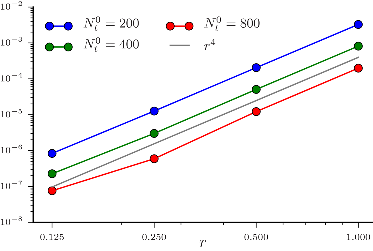
 . Figure 19 shows the convergence of the growth rate of the two-stream instability as the grid is refined. Since the solver is only second order in time, the time step must be reduced quadratically while the phase-space grid spacing is scaled linearly to achieve overall fourth-order convergence.
Convergence of the two-stream growth rate for the higher-order solver as the grid parameters are scaled as $N_x=r N_x^{0}$ , $N_v=rN_v^{0}$
 and $N_t = r^{2}N_t^{0}$
 for various values of $N_t^{0}$
 with $N_x^{0} = 32$
 and $N_v^{0}=201$
 .
.
Furthermore, both updates are time reversible, that is, in both (3.1) and (3.24), with the replacement ${{\Delta t}} \rightarrow -{{\Delta t}}$ , the corresponding algorithms take ${f}^{n+1}_{{k}{j}}$
 to ${f}^{n}_{{k}{j}}$
 . This means that composition techniques (Suzuki Reference Suzuki1990; Yoshida Reference Yoshida1990; Suzuki & Umeno Reference Suzuki and Umeno1993; McLachlan Reference McLachlan1995; Hairer et al. Reference Hairer, Lubich and Wanner2002) can be used to construct algorithms that are higher order in time. Importantly, the composition will preserve all conservation properties of the basic method. As a demonstration, we start with the split algorithm and construct various higher-order methods. Let $S^{({2})}({{\Delta t}})$
 be the operator corresponding to the update (3.24). Composing three applications of $S^{({2})}$
 yields a fourth-order accurate time-update (Yoshida Reference Yoshida1990)

where $a_1 = 1/(2 - 2^{1/3})$ and $a_0 = 1 - 2a_1$
 . In turn, $S^{({4})}$
 can be used in a three-step composition producing a sixth-order update (Yoshida Reference Yoshida1990)

where $b_1 = 1/(2 - 2^{1/5})$ and $b_0 = 1 - 2b_1$
 . This sequence can be continued to obtain any even order. Evidently, a single step of $S^{({4})}$
 is three times the work of an $S^{({2})}$
 step while a single step of $S^{({6})}$
 is nine times the work. At sixth order, more efficient compositions are possible; for example (Yoshida Reference Yoshida1990)

where
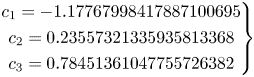
and $c_0 = 1 - 2(c_1 + c_2 + c_3)$ only requires seven evaluations of $S^{({2})}$
 and has better truncation error (McLachlan Reference McLachlan1995). To illustrate these higher-order methods, we consider a weakly nonlinear Landau damping example with $A = 0.15$
 , ${k\lambda _D} = 0.4$
 , spatial domain $[0, 10{\rm \pi} \lambda _D]$
 , velocity domain $[-10{v_\mathrm {th}}, 10{v_\mathrm {th}}]$
 , ${{N_x}} = 1024$
 and ${{N_v}} = 2001$
 . Figure 20 shows the absolute relative energy error in the solutions obtained from these higher-order methods, as well as from $S^{({2})}$
 for comparison. The scaling of the energy error for all methods is consistent with the order (most easily seen by comparing with scaling for $S^{({2})}$
 ). As expected, the higher-order methods outperform lower-order methods as the accuracy increases. For example, the energy error obtained by $S^{({4})}$
 with $\omega _p{{\Delta t}}=0.0625$
 is comparable to that of $S^{({6'})}$
 with $\omega _p{{\Delta t}}=0.25$
 while the latter method requires $7/12$
 the computational work of the former. For a given value of ${{\Delta t}}$
 , the energy error in the solution from $S^{({6'})}$
 is significantly smaller than that from $S^{({6})}$
 which is consistent with the optimization used in construction of $S^{({6'})}$
 (McLachlan Reference McLachlan1995). The composition rules used here all rely on the exact reversibility of the underlying update algorithm $S^{({2})}$
 . In general, the numerical solution of the linear systems in (3.24) will have a residual larger than machine precision which implies that the reversibility of the advance will hold only to some multiple of machine precision. In fact, for the parameters used in this example, an optimized eighth-order composition (Suzuki & Umeno Reference Suzuki and Umeno1993; McLachlan Reference McLachlan1995) (not shown) did not yield much improvement in error beyond that of $S^{({6'})}$
 . Thus there will be a limit on the order than can be obtained by such composition rules. (Presumably through iterative refinement (Moler Reference Moler1967) of the linear system solutions this limit could be raised.) Further, increasing the discretization accuracy on phase space would be expected to lower the size of the linear systems in (3.24), leading to lower residuals possibly allowing even higher-order composition than considered here; this will be the topic of a future publication.
Absolute relative energy error for weakly nonlinear Landau damping for different order methods and various values of $\omega _p{{\Delta t}}$ . See text for parameters. The column labelled ‘O’ identifies the method.

6. Conclusions
We have developed an implicit, unconditionally stable numerical scheme to solve the Vlasov–Poisson system in one dimension. This method uses a Crank–Nicolson discretization scheme for the time discretization, and Strang splitting to effectively remove the nonlinear coupling between the field and distribution function. The splitting results in low-bandwidth linear systems that are suitable for direction solution. This algorithm exactly conserves particle number, enstrophy and momentum; the unsplit form also exactly conserves energy. This method is essentially non-dissipative and so rapid variations of the distribution function in phase space can induce oscillations, and positivity of $f$ is not maintained. However, we have shown that this effect is relatively benign for the systems consider herein.
We presented a thorough analysis of the algorithm beginning with phase space discretization and continuous time. We show that the introduction of a phase-space grid leaves energy and momentum conservation intact but with particle number and enstropy being the only surviving Casimirs. In the transition to discrete time, we show that the Crank–Nicolson discretization preserves all of the invariants that survive phase-space discretization. With the introduction of Strang splitting, exact energy conservation is lost. The exact conservation of enstrophy guarantees nonlinear numerical stability. The split form of this algorithm has been extended to the relativistic Vlasov–Poisson system (Carrié & Shadwick Reference Carrié and Shadwick2016), yielding identical conservation and stability properties.
We considered a number of widely used test cases and demonstrated that the algorithm is second order in phase space and time. We show that for Landau damping, a linearized version of the algorithm converges to the van Kampen solution. The results for nonlinear Landau damping are in good agreement with the existing literature. For the two-stream problem we show that the fundamental mode agrees very well with the linear theory until quite close to saturation. Taking advantage of the quadratic convergence of the algorithm we obtained converged growth rates by extrapolating to infinite resolution.
This method has an obvious extension to higher-order differencing in phase space. Provided central differences are used, the conservation properties will be unchanged. We have demonstrated methods using fourth-order central differences in phase space and higher order in time by using standard composition techniques (Suzuki Reference Suzuki1990; Yoshida Reference Yoshida1990). In either case, the conservation (and consequently stability) properties persist. There is no technical limitation on using the composition techniques with higher-order phase-space differencing.
All code and data used in this manuscript are available from the corresponding author.
Acknowledgements
The authors gratefully acknowledge helpful conversations with P.J. Morrison, J.M. Finn, C.B. Schroeder and B. Afeyan.
Editor W. Dorland thanks the referees for their advice in evaluating this article.
Funding
The work was supported by Department of Energy (contract numbers DE-FG02-08ER 55000 and DE-SC0008382); and by the National Science Foundation (grant number PHY-1104683). B.A.S. was supported by the National Science Foundation under grant no. DMS-1440140 while in residence at the Mathematical Sciences Research Institute in Berkeley, California, during the Fall 2018 semester.
Declaration of interests
The authors report no conflict of interest.
Appendix A. Properties of the phase-space discretization
The advection operators (2.3) and (2.4) have a number of properties that are central the results of §§ 2 and 3. Consider

Our spatial domain is periodic so we can interpret spatial indices modulo ${{N_x}}$ and hence the spatial index can be shifted by any amount without altering the sum. Thus the two sums in (A1) cancel giving

Now

Spatial periodicity forces these two sums to cancel and we have

Consider

where we have used spatial periodicity to shift the sums. Consider
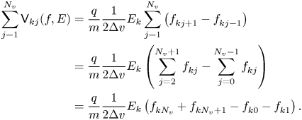
Our boundary conditions in $v$ imply ${f}^{}_{{k}{{{N_v}}+1}} = 0 = {f}^{}_{{k}{0}}$
 and we have

Now consider

Using our boundary conditions in $v$ and the fact that velocity grid has uniform spacing ${{\Delta v}}$
 , this becomes
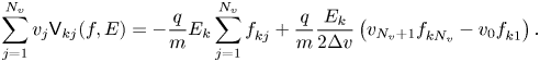
Now
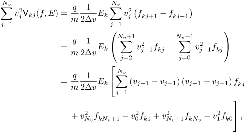
taking into account the boundary conditions and uniform $v$ grid, we find

Lastly consider

which, given our boundary conditions, becomes

These results all generalize straightforwardly to higher-order centred-difference approxi- mations for the derivatives in $\mathsf {S}_{kj}$ and $\mathsf {V} _{kj}$
 .
.
Appendix B. Linearization
Linearizing about a spatially uniform equilibrium $f^{(0)}_{0}$ , we have
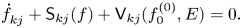
where $f$ now represents the first-order departure of the distribution function from $f^{(0)}_{0}$
 and $E$
 is the linearized electric field. Since the spatial domain is periodic, $\sum _{k=1}^{N_x} E_k = 0$
 and thus

leading to conservation of particle number and momentum in the continuous-time case. In the linearized case, the correct energy expression is the Kruskal–Oberman energy (Kruskal & Oberman Reference Kruskal and Oberman1958; Morrison & Pfirsch Reference Morrison and Pfirsch1990):

With the introduction of a phase-space grid this becomes

and


From (A4), we see that ${\textrm {d}}\mathscr {E}_\mathrm {KO}/{\textrm {d}}t = 0$ .
.
We solve the linearized equations with our split-step algorithm, (3.24), where we replace (3.24b) with

and (3.24d) with

As in the nonlinear case, this algorithm exactly conserves particle number and momentum, while the Kruskal–Oberman energy is only approximately conserved.
Assuming temporal and spatial dependencies of the form $\textrm {e}^{-\textrm {i}\omega t}$ and $\textrm {e}^{\textrm {i} kx}$
 , respectively, leads, in the usual way (Krall & Trivelpiece Reference Krall and Trivelpiece1973), to the plasma dielectric function, defined for $\omega _i > 0$
 as
as

For $\omega _i < 0$ , $\epsilon$
 can be obtained from the relationship $\epsilon (k, \omega )^{*} = \epsilon (k, \omega ^{*})$
 . Zeros of $\epsilon$
 correspond to normal modes of the system. In addition to such modes, in the asymptotic limit, the initial value problem can also give rise to wave-like solutions (Landau Reference Landau1946; van Kampen & Felderhof Reference van Kampen and Felderhof1967). This asymptotic behaviour is governed by roots in the lower half-plane of the analytic continuation of $\epsilon$
 , $\varXi$
 . Following Gakhov (Reference Gakhov1990), we have

For the Maxwellian equilibrium (4.2), the dielectric function becomes

While this can be expressed in terms of the plasma dispersion function (Fried & Conte Reference Fried and Conte1961), it is more convenient to write $\epsilon$ , for $\omega _i > 0$
 , as
, as

For real $\omega$ , we have

where $\omega _i \rightarrow 0^{\pm }$ and $\operatorname {daw}(x)$
 is Dawson's integral (Abramowitz & Stegun Reference Abramowitz and Stegun1964).
For the two-stream equilibrium (4.15), the dielectric function becomes

for $\omega _i > 0$ . For real $\omega$
 , we have

where $\omega _i \rightarrow 0^{\pm }$ . The Penrose condition (Penrose Reference Penrose1960) shows that this equilibrium is unstable for any $v_0$
 . The spectrum of unstable modes is found by solving $\epsilon = 0$
 with $\omega$
 in the upper half-plane. Figure 21 shows $\omega _i$
 for the two-stream problem; $\omega _r = 0$
 for all unstable modes. The largest value of $k$
 giving an instability is $\omega _p/v_0 = \sqrt {3}/\lambda _D$
 .
.
Growth rate of the two-stream instability. The maximum growth rate occurs at $k \approx 0.43\omega _p/v_0$ .
.


 Open access