


1. INTRODUCTION
Mass-balance studies address the spatial and temporal changes in the ice mass of a glacier. Winter snowfall and summer temperature alter the amount of snow collected on the glacier and the amount of snow and ice lost by melt, thus changes in glacier mass are linked to changes in climate. Changes in the mass balance influence the dynamics of the glacier, which results in a change in the position of the glacier terminus (Paterson, Reference Paterson1994). Because of the relation between glacier geometry and climate, are glaciers seen as important indicators of climate change.
There are five commonly used methods for measuring the mass changes of the glaciers (Vaughan and others, Reference Vaughan, Stocker, Qin, Pslattner, Tignor, Allen, Boschung, Nauels, Xia, Bex and Midgley2013). Traditionally, the mass balance is observed using the glaciological method, i.e. the mass balance is derived from repeated stake measurements of snow and ice surface. The surface elevation changes are summed to give the total surface mass balance (SMB). In the glaciological method pointwise measurements are generalized to represent larger areas of the glacier, and estimates of the net mass balance (B n) are deduced. However, local climate and glacial processes can create significant spatial differences in the SMB. Drifting snow, avalanching and shading by surrounding mountains can affect the accumulation and ablation patterns of a glacier, and thus localized observations can lead to biases in the estimate of mass balance (Barrand and others, Reference Barrand, Murray and James2010). The second method, often referred to as the geodetic method (Barrand and others, Reference Barrand, Murray and James2010), converts observed volume changes of the glacier to mass change. Surface elevation changes are obtained from repeated elevation profiles or DEMs. The geodetic mass balance derived from full coverage DEMs provides a better means to assess the spatial variations of the SMB. Nevertheless, the method is unable to reveal whether the local surface elevation changes are caused by accumulation, melt, or glacier flow redistributing the ice. The conversion from volume to mass is also prone to errors due to the limited information on snow and firn density on glaciers (Gardner and others, Reference Gardner2013). Since the successful launch of the Gravity Recovery and Climate Experiment (GRACE)-mission in 2003, mass changes of land ice can be estimated from satellite measurements of gravity field. However, due to the coarse spatial resolution, this third method is not applicable to small glaciers but rather is most suitable for total ice-sheet balances (Gardner and others, Reference Gardner2013). The fourth method comprises different mass-balance modelling approaches that convert time series of meteorological variables, or changes in glacier length or equilibrium line altitude, to mass changes. Vaughan and others (Reference Vaughan, Stocker, Qin, Pslattner, Tignor, Allen, Boschung, Nauels, Xia, Bex and Midgley2013) assume that the improvements in this type of models can advance the estimation of mass changes. As a fifth alternative, it is possible to determine glacier mass balance as a residual of the water balance for the basin tributary to the glacier terminus.
Midtre Lovénbreen (ML), with an area of 5.4 km2 and an elevation range from 50 to 650 m a.s.l. in year 2001, is a thoroughly studied valley glacier in Svalbard (78.53°N, 12.04°E). Located near the settlement of Ny-Ålesund, ML has been subject of numerous studies and long-term monitoring. Annual mass balance has been measured since 1968 by the Norwegian Polar Institute, and flow velocity measurements have been carried out since the 2000s. In this study we use velocity measurements from 2005 to 2006 to evaluate the modelled velocities. Continuous meteorological measurements by the Norwegian Meteorological Institute are available in Ny-Ålesund since 1974. ML offers a good test case for numerical experiments owing to the availability of in situ observations that can be applied to evaluate the model results.
Surface elevation and corresponding mass-balance changes at ML-based on stake measurements or DEMs have been addressed in several previous studies (Dyurgerov and Meier, Reference Dyurgerov and Meier2000; Rippin and others, Reference Rippin2003; Kohler and others, Reference Kohler2007; Barrand and others, Reference Barrand, Murray, James, Barr and Mills2009, Reference Barrand, Murray and James2010; James and others, Reference James2012). A mass balance model for ML has been presented by Rye and others (Reference Rye, Arnold, Willis and Kohler2010), who found that the method gave sufficiently good results. However, their model is forced by coarse horizontal resolution (ca. 125 km) ERA-40 reanalysis, and requires bias correction of the forcing fields as well as substantial model calibration, which limits the applicability and reliability of the model.
In this study we use the high-resolution full-stress ice flow model Elmer/Ice (Gagliardini and others, Reference Gagliardini2013). In contrast to a previous application using the same model that focused on a prognostic simulation of ML (Zwinger and Moore, Reference Zwinger and Moore2009), we develop a method inspired by inverse modelling to resolve the past SMB distribution over the glacier. We present a modelled solution of SMB for four time periods from 1962 to 2005, show the temporal evolution of the SMB, and evaluate the modelled results against observations.
2. OBSERVATIONAL DATA
The main input data for our study are surface DEMs for ML, based on maps and data from 1962, 1969, 1977, 1995 and 2005 (Kohler and others, Reference Kohler2007). The 1962 DEM is derived from a 10 m contour map based on oblique terrestrial photogrammetry (Pillewizer, Reference Pillewizer1962). The 1969 and 1977 DEMs are derived from unpublished NPI maps made from vertical aerial photographs (Kohler and others, Reference Kohler2007). For these first three DEMs, contours were digitized from paper maps, converted to a common datum and projection (WGS84, UTM zone 33 north), and surface data interpolated onto a 5 m grid. The 1995 DEM was directly obtained with digital photogrammetry from vertical aerial photographs, with an original resolution of 5 m. The 2005 DEM was derived from an airborne Lidar campaign (James and others, Reference James, Murray, Barrand and Barr2006), with data interpolated to the 5 m grid. To obtain ice thickness for each epoch, we subtract elevations of each surface DEM from the bedrock DEM created from ground-penetrating radar data (Rippin and others, Reference Rippin2003; Zwinger and Moore, Reference Zwinger and Moore2009).
The uncertainties of the surface DEMs are quantified by analyzing the map differences in the ice-free areas between year 2005 and the rest of the years. The bias of the DEM is based on the standard deviation of the maps differences in the areas where the slope is <20°. In addition the standard deviation relative to year 2005 the total bias contains map errors and the geoid-ellipsoid error, which are included in the error estimate. The errors for the map pairs are shown in Table 1. The uncertainties of the DEMs are largest for the oldest DEM pair and smallest for the two most recent pairs. In 1962–69 the error (in m a−1) was five times larger than in 1977–95 and 1995–2005. The model results directly rely on the measured geometry of the glacier, thus the modelled SMB is expected to be sensitive to the uncertainties in the DEMs. To study the sensitivity of the model to the DEM uncertainties we perform two additional simulations for each DEM pair where we add and subtract the mean DEM error from the mean surface of the glacier. The sensitivity runs are described in Section 3.
DEM uncertainties and mass-balance sensitivity to the DEM uncertainties
We compare the 2005 simulated surface velocity to data obtained that same year at 17 stake positions. The locations of the measurement stakes are shown in Figure 1. The stakes are mainly located along the glacier centerline, with six stakes off the centerline. While winter and summer data are available, we use the annual velocities (May 2005–May 2006) to compare with the model results. Velocities are derived from repeated differential GPS surveys of the stake positions, and have a nominal accuracy of ca. 0.1 m a−1.
Locations of the measurement stakes in spring 2005 (black dots). The darker gray denotes the shape of the glacier in 1962 and the lighter gray in 2005.
Continuous monitoring of the glacier's mass balance started in the year 1967 using the direct glaciological method (Hagen and Liestøl, Reference Hagen and Liestøl1990). The in situ observations along the centerline are interpolated over the elevation range of the glacier weighted by the hypsometry.
3. METHODS
In this study we combine observed surface elevation and bedrock data with the solution of a diagnostic ice flow model in order to inversely determine the accumulation and melt. We use the ice-dynamic model Elmer/Ice (Gagliardini and others, Reference Gagliardini2013), which solves the full Stokes equations. The increased complexity and effort to solve the full Stokes equations compared with models applying approximations linked to thin film flow are negligible, as the present study only applies diagnostic (i.e., time-independent) simulations, which requires no significant computing time.
3.1. Ice flow model
The flow is governed by the balance of the divergence of the Cauchy stress, σ and the specific weight given by density times gravity, ρ g,
 $$\nabla \cdot {\bi \sigma} + \rho {\bi g} = {\bf 0},$$
forming a set of three equations, one for each direction {x, y, z} of a Cartesian coordinate system. In the model output, the x-coordinate is pointing to the east and y-coordinate to the north. The z-coordinate is normal to the glacier surface and directed upward from the surface. The Cauchy stress tensor, σ = τ − p I, where I is the identity tensor, usually is split into its isotropic part, the pressure p = −trσ/3 and the deviatoric stress, τ, for which a closure relation,
 $${\bi \tau} = 2\eta \dot {\it \epsilon}, $$
gives the six independent coefficients (τ xx, τ yy, τ zz, τ xy, τ xz, τ yz) as a function of the strain-rate tensor,
 $$\dot {\it \epsilon} = \displaystyle{1 \over 2}(\nabla {\bi u} + (\nabla {\bi u})^T ){\rm.} $$
 In other words, we replace the deviatoric stress-tensor by the gradient of the unknown velocity u = (u, v, w)T. The effective viscosity, η, itself is dependent on the temperature relative to pressure melting point, T′ and the effective strain rate (the second invariant of the strain rate tensor),  $\dot {\it \epsilon} _{{\rm eff}} = \sqrt {{\rm tr}\dot {\it \epsilon} ^2} $ in the form of a general Norton–Hoff power law. In glaciology, the exponent n is set to 3, and the resulting equation is known as Glen's flow law (Paterson, Reference Paterson1994):
 $$\eta (T^{\prime},\dot {\it \epsilon} _{{\rm eff}} ) = \displaystyle{1 \over 2}(EA(T^{\prime}))^{ - 1/n} \dot {\it \epsilon} _{{\rm eff}}^{(1 - n)/n}. $$
 The enhancement factor in our simulations is kept at constant E = 1 and the rate factor  $A(T') = 2.05 \times 10^{ - 24} {\kern 1pt} {\rm s}^{ - 1} {\rm Pa}^{ - 3} $, resembling a constant relative temperature of $T' = - 1{\kern -1pt}$°C. This can be justified by earlier thermo-mechanically coupled diagnostic simulations of ML (Zwinger and Moore, Reference Zwinger and Moore2009) that revealed a core temperature in the range from −2 to 0°C for large parts of the glacier. Further, runs with lower temperatures showed velocities well below the observed. Velocity components and pressure form a set of four unknowns, which, besides the three components of the momentum balance (Eqn 1), demands the inclusion of the mass or volume balance for incompressible flow, as firn is not accounted for in these simulations
 $${\rm tr}\dot {\it \epsilon} = \nabla \cdot {\bi u} = 0.$$
These equations are then solved for a surface geometry z = h(x, y;t 0) at a given time t 0, with the bedrock geometry z = b(x, y) assumed to be constant over the time span of interest. Eqns (1) and (5) are completed by boundary conditions at the bedrock and the free surface. At the free surface we impose a vanishing stress vector
 $${\bi T} = {\bi \sigma} \cdot {\bi n}_{\rm s} = {\bf 0},$$
where ns is the upward normal vector of the free surface. As the additional kinematic boundary condition at the free surface will be used to determine the SMB, it will be discussed in detail later. At the bedrock we impose the condition that there is no penetration of ice into the subsurface:
 $${\bi u} \cdot {\bi n}_{\rm b} = 0,$$
where nb is the outward pointing normal vector of the bedrock surface.
A reference run with no basal sliding showed that ice velocities were slower than those observed. Consequently, for the tangential component of the velocity vector,  ${\bi u}_{\rm \parallel} = {\bi u} - ({\bi u} \cdot {\bi n}_{\rm b} ){\bi n}_{\rm b} $, we impose a linear sliding relation,
 $${\bi u}_{\rm \parallel} = c^{ - 1} {\bi T}_{\rm \parallel}, $$
where  ${\bi T}_{\rm \parallel} $ is the tangential component of the stress vector at the bedrock. The friction coefficient is set as a function of ice thickness, d,
 $$c = \left\{ {\matrix{ {0.0013\;{\rm Pa}\;{\rm s}\;{\rm m}^{ - 1}} & {{\rm if}\;d \ge 120\;{\rm m}} \cr {0.32\;{\rm Pa}\;{\rm s}\;{\rm m}^{ - 1}} & {{\rm if}\;d \lt 120\;{\rm m}} \cr}} \right.$$
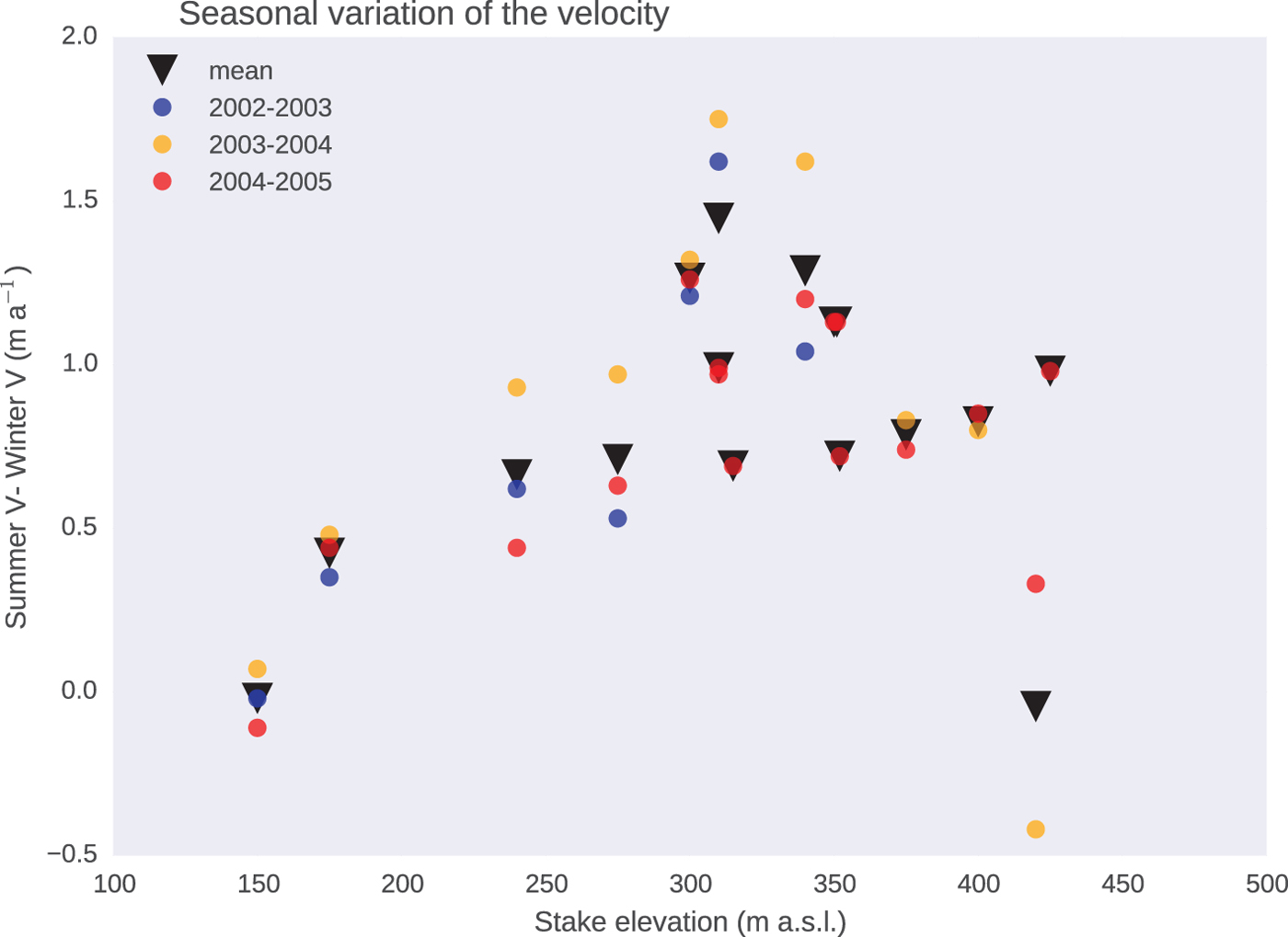
This sets a small sliding component over the deeper parts of the glacier, whereas the high value of c over the shallower parts resembles a no-slip condition. We adopted a thickness dependent sliding since the impact of the velocity to the volume change is highest where the ice is thickest. Even the seemingly hard transition in the friction coefficient provides smooth change in the surface velocity field. The friction coefficient for the areas subject to sliding was determined by comparing the modelled velocities with the observed velocities at the stake locations. The friction coefficient was empirically chosen from a series of test simulations in order to minimize the error between the simulated and observed velocities. Including basal sliding in addition to the internal deformation can be justified by the observation that velocities in the thicker parts of the glacier show a significant increase in summer compared with winter, and that there is significant interannual variability, which can be linked to the change of basal conditions and occurence of sliding. Figure 2 shows the difference between summer and winter velocity during mass-balance years 2002/03, 2003/04 and 2004/05. The velocity increases in summer compared with winter at the elevations of 250–400 m a.s.l., which roughly correspond to the deepest parts of the glacier.
The difference between summer and winter velocity at the measurement stakes during mass-balance years 2002/03, 2003/04 and 2004/05.
3.2. Obtaining the SMB pattern
Using the set of given surface DEMs, we pick two consecutive configurations, h(t 1) and h(t 2), with t 1 < t 2, to compute an averaged surface elevation distribution, using their arithmetic mean value for each position (x, y) on the glacier,
 $$h_{t_1 \to t_2} (x,y) = \displaystyle{1 \over 2}\left[ {h_{t_1} (x,y) + h_{t_2} (x,y)} \right].$$
By approximating a linear temporal evolution of the free surface between these times,
 $$\displaystyle{{\partial h_{t_1 \to t_2}} \over {\partial t}} = \displaystyle{{h_{t_2} - h_{t_1}} \over {t_2 - t_1}}, $$
we can interpret Eqn (10) as the elevation distribution at the time t 1→2 = 1/2(t 1 + t 2). The kinematic boundary condition links the local as well as convective change caused by the surface velocity (u h, v h, w h)T of surface elevation to the net accumulation normal to the glacier surface, a ⊥. Given that the average slope on ML is small, 8°, the difference between a height measured normal to the surface (as in our model) or straight up from the surface (as at the measurement stakes) is ~1%. The kinematic boundary condition then reads as (Greve and Blatter, Reference Greve and Blatter2009),
 $$\displaystyle{{\partial h} \over {\partial t}} + u_h \displaystyle{{\partial h} \over {\partial x}} + v_h \displaystyle{{\partial h} \over {\partial y}} - w_h = a_ \bot. $$
 In order to determine the average net SMB  $(a_{t_1 \to t_2} (x,y))$ for the time period t 1 → t 2, the first term in Eqn (12) is approximated using expression Eqn (11) and the horizontal (x, y) components of the surface gradient by $\nabla h \approx \nabla h_{t_1 \to t_2} $. The velocities required in the last three terms of the left hand side of Eqn (12) are computed by a diagnostic (i.e., steady state) simulation of the ice flow model under the given surface geometry $h_{t_1 \to t_2} $.
Using the expression for the emergence velocity,
 $${\bi u}_{{\rm em}} (h,{\bi u}) = w_h - u_h \displaystyle{{\partial h} \over {\partial x}} - v_h \displaystyle{{\partial h} \over {\partial y}},$$
one then can express the solution for the SMB accumulation and ablation needed to be applied to evolve the glacier surface from  $h_{t_1} (x,y;t = t_1 )$ to $h_{t_2} (x,y;t = t_2 )$:
 $$a_ \bot ^{(t_1 \to t_2 )} = \displaystyle{{\partial h_{t_1 \to t_2}} \over {\partial t}} - {\bi u}_{{\rm em}} (h_{t_1 \to t_2}, {\bi u}).$$
4. RESULTS
4.1. Evaluation of modelled velocities
We evaluate the quality of our modelled velocity field with simulations performed using the DEM from the year 2005, which can be compared with measured values at stake positions obtained in the month of May of the same as well as the following year.
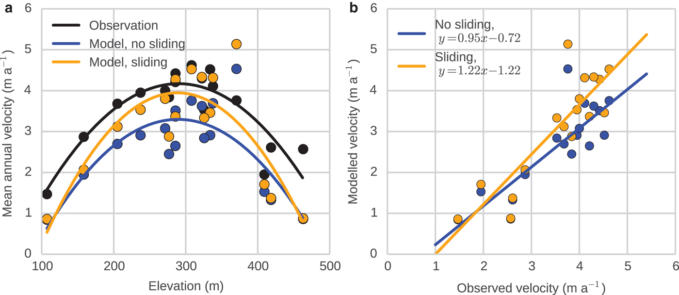
We perform two simulations, one assuming a frozen bed, i.e. setting the ice velocity to zero at the bottom boundary. In the second simulation slip conditions were introduced over certain regions of the glacier bed following Eqn (9). In the latter, sliding is applied only at the locations where the thickness of the glacier exceeds 120 m, thereby limiting it to the central parts. Observed and modelled horizontal velocities at the stake positions as a function of elevation are presented in Figure 3. The horizontal surface velocities are fastest over the central parts of the glacier, reaching ~4.5 m a−1 in the observations. Both simulations have an overall slow bias of −0.9 and −0.4 m a−1 for simulations with no-slip and thickness-dependent sliding, respectively. Even though the latter reduces the velocity bias over the central parts of the glacier, it also exaggerates the velocity difference between the tongue, mid-elevation and accumulation area. Figure 3 clearly illustrates the problem: while the mean bias decreases when basal sliding is allowed, the slope of the linear fit between observed and modelled velocities (Fig. 3b) grows and deviates more strongly from the target unity-value than the one obtained without sliding. Hence we chose not to further increase sliding speeds by introducing even lower friction coefficients.
Modelled and observed velocities in 2005. Panel (a) shows the observed velocities in function of elevation (black dots) and a second degree polynomial fit (black line). Similarly, it shows the modelled surface velocities from the stake locations from the frozen bed (blue) and bottom sliding (orange) simulations. Panel (b) presents scatter plots of observed and modelled velocities for the model experiments of frozen bed (blue dots) and basal sliding (orange dots). Lines in panel (b) indicate the linear fits to the points.
We assume that the velocity biases between the simulation and measurements for 2005 are similar for the configurations of the older time periods, however we acknowledge that the quality of the DEMs and possible changes in glacier temperature and basal conditions can affect the performance of the model.
4.2. Modelled evolution of SMB
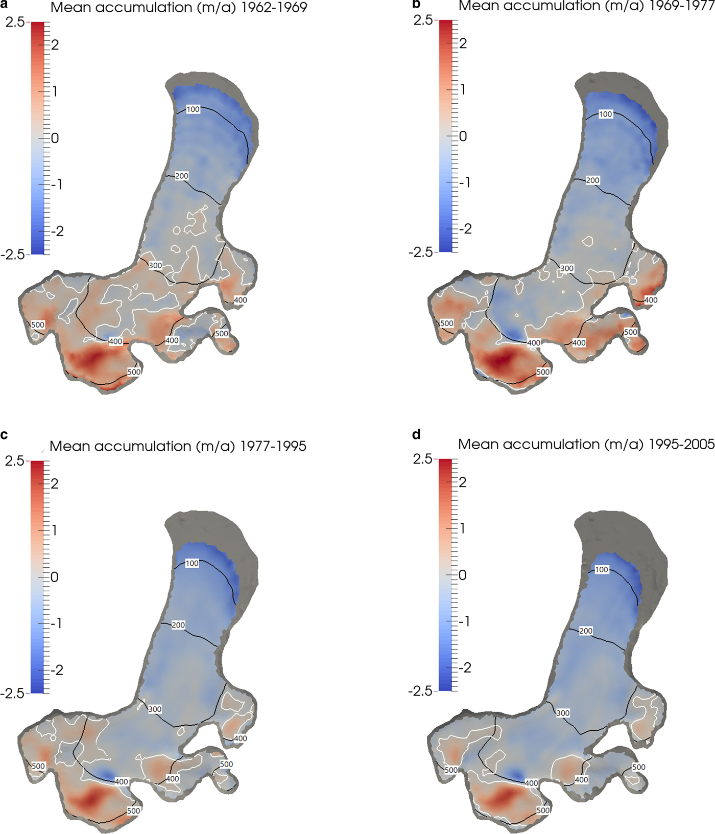
Average net accumulation, a ⊥, (equivalent to SMB) distributions for the time intervals 1962–69, 1969–77, 1977–95, and 1995–2005 are calculated using the kinematic free surface equation [Eqn (14)]. The patterns are shown in Figure 4. During the study period the accumulation area has decreased and the zero contour of accumulation, equivalent to the equilibrium line altitude (ELA), has ascended. According to the model results the zero contour was at ~250 m in 1962–69. The simulation obtained from the DEMs of 1969 and 1977 revealed an increase of the ELA by 100–350 m, a further increase to 400 m in 1977–95, and to 450 m in 1995–2005.
Charts of modelled mean accumulation or ablation in 1962–69, 1969–77, 1977–95 and 1995–2005 with the blue-red color scale. Solid white lines show the zero contour of accumulation, which can be interpreted as the equilibrium line altitude. Black contours denote the surface elevation in m.a.s.l. Grey background area indicates the outline of the glacier in 1962, the maximum extent of the modelling domain. All units are m a−1 ice equivalent.
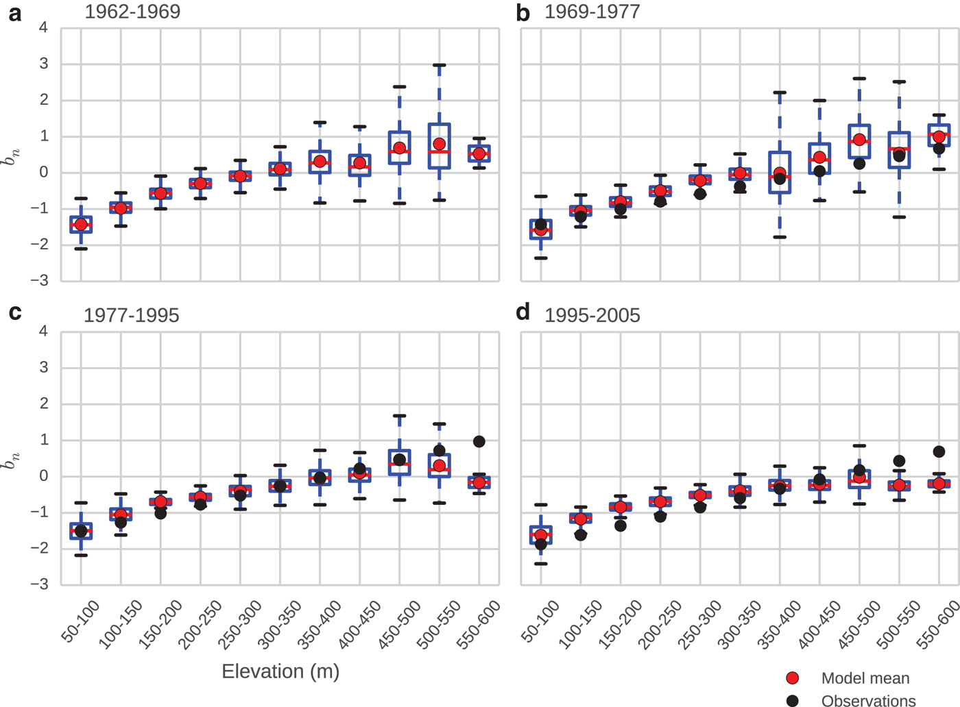
The boxplots in Figure 5 show the altitudinal distribution of the SMB for the four time intervals. In each panel of the figures, the model output SMB is separated into bins based on the surface elevation. Each bin covers a 50 m elevation range such that the lowest bin ranges from 50 to 100 m a.s.l., and the highest from 550 to 600 m a.s.l. The number of gridpoints in each elevation bin is indicated in Table 2. The basic statistics are calculated for the modelled value of a ⊥ in each bin. Here, the simulated mean accumulation over the elevation bins, b n, is defined as:
 $$b_n = \displaystyle{1 \over N}\sum\limits_{i = 1}^N a_{ \bot i}^{(t_1 \to t_2 )}. $$
Boxplots of the modelled and measured accumulation in function of elevation. Red lines show the median and red dots mean modelled SMB at the given elevation range. Blue boxes show the upper and lower quartile and black whiskers show 1.5 times the interquartile range. Black dots are the observed or the interpolation of the observed SMB. b n is given in meters of ice.
Number of points in each elevation bin of the boxplots
Inside each elevation bin, values of a ⊥ are not always normally distributed. This results in a deviation of the mean and the median as well as differences in the distribution below and above the median. The measured mass balances, reported in m w.e. a−1, have been translated to meters of ice by multiplying with a factor of 1.09 (the ratio of water to the density of ice, ρ w/ρ i, (Hooke, Reference Hooke2005)). Mass-balance observations only start in 1967/68, hence they do not show in the first graph (1962–69).
In 1962–69 (Fig. 5a) the strongest ablation is ~−1.5 m of ice a−1 and the highest value of accumulation ~0.8 m of ice a−1. The maximum values occur in the 500–550 m bin, rather than in the highest elevated at 550–600 m. In the ablation area, from the 250 to 300 m bin downward, ablation decreases more or less linearly with elevation. At higher elevations, the spread in modelled values grows significantly. Large variability in the accumulation area might reflect a large spatial variability in snow accumulation, or may be an artifact of uncertainties in the DEMs or changes in the the densification of firn.
The modelled SMB profile in 1969–77 (Fig. 5b) shows a generally similar distribution to that of 1962–69 in terms of linear decrease of ablation from the glacier tongue up to the ELA (here 350 m) and large spread in the accumulation area. In Figure 5b) we also include the measured glaciological mass balance. Observations closely match the modelled mean in the ablation area especially at 100–250 m a.s.l. whereas in the accumulation area modelled mean values exceed the measurements on average by 0.5 m of ice a−1.
In 1977–95 (Fig. 5c) we see an overall increase in modelled ablation with respect to the earlier period. Modelled and observed SMB values match closely from 200 to 500 m. From 500 to 600 m the modelled SMB drops below the observed SMB and in the 550–600 m bin the difference is close to 1 m of ice a−1, with the observed value even falling outside the upper bound of the spread indicated by the model. The modelled a ⊥ variability inside the elevation bins is smaller than in the two previous time periods. The variability of the modelled results might be reduced by more accurate DEMs, but as will be explained below, observed mass-balance values in the highest elevation bins are extrapolated, and thus are more uncertain than the model results.
For the time period of 1995–2005 (Fig. 5d) the model median a ⊥ is negative all over the glacier. At 100–350 m elevation the model mean is higher than the observed, whereas at 450–600 m mean modelled SMB is lower than the observations. The spatial variability of modelled a ⊥ inside the elevation bins is the smallest of all the four time periods.
As expected, results presented in Figure 5 show a rising ELA and decreasing SMB over time. The two earlier time periods have a larger spread in the modelled a ⊥ than the two more recent simulations. This might be related to the better accuracy of the more recent DEMs. In 1977–95 and 1995–2005 the mean and median a ⊥ are lower than observed at the highest parts of the accumulation area. As the model input DEMs are relatively reliable in these recent simulations, the mismatch with observations may be due to the interpolation of the in-situ measurements.
Glaciological mass balance, geodetic mass balance, modelled net accumulation (a ⊥) and modelled and observed ELA are given in Table 3. As the glaciological mass-balance measurements start from 1967/68, glaciological data are not presented for 1962–69. All records of measured mass balance and modelled net accumulation are negative. Modelled a ⊥ shows a continuous decrease, whereas observational data show a weak increase in mass balance in 1977–95 compared with 1969–77. The time series of annual mass-balance observations from 1968 to 2012, not averaged to our study periods, do not show a statistically significant trend.
Glaciological net mass balance (B n), geodetic net mass balance, modelled net accumulation  $(a_ \bot ^{(t_1 \to t_2 )} )$ and modelled and observed ELA. Observed ELA is based on linear fit to measurements at stake locations. Modelled ELA is calculated as a linear fit to modelled data selected from stake location (‘points’) and linear fit to mean SMB in elevation bins of 50 m altitude range (‘bins’)
Table 3 also indicates the mean model-derived ELA for the different time periods. The observed ELA is based on an interpolation of stake measurements. The annual ELA observations are averaged over time periods of the simulations. Observed ELA varies from 380 to 440 m. To compare the modelled ELA to measurements, we selected the modelled a ⊥ from stake locations and performed a linear fit in function of elevation, from which the ‘Modelled ELA, points’ are deduced. The values are comparable with the measurements, but as for mean a ⊥, modelled ELA increases steadily over time, whereas observed ELA also decreases relative to the previous period in 1977–95. Finally, we use the mean modelled values of a ⊥ in 50 m elevation bins, presented also in Figure 5. ‘Modelled ELA, bins’ is estimated based on a linear fit to the mean a ⊥ of the bins. Again, values differ from the point methods and the measurements, but are of the same order of magnitude.
4.3. Sensitivity of the modelled mass balance to the uncertainties of the DEMs
The model relies on the measured geometry of the glacier and thus the modelled SMB is sensitive to the errors in the DEMs (Table 1). To study the sensitivity of the model to the DEM uncertainties we perform for each DEM pair two additional simulations where we add and subtract the mean DEM error from the mean surface of the glacier. The results give us two new SMB fields for each DEM pair. We calculate the SMB error as the difference of the two SMB fields. We further calculate also the mean error as the average of the SMB difference over the glacier (Table 1). The error of the modelled SMB decreases together with the uncertainty of the DEM. In the simulation of 1962–69 the mean SMB error between two sensitivity simulations was ±0.93 m, and in 1995–2005 the error difference was reduced to ±0.17 m.
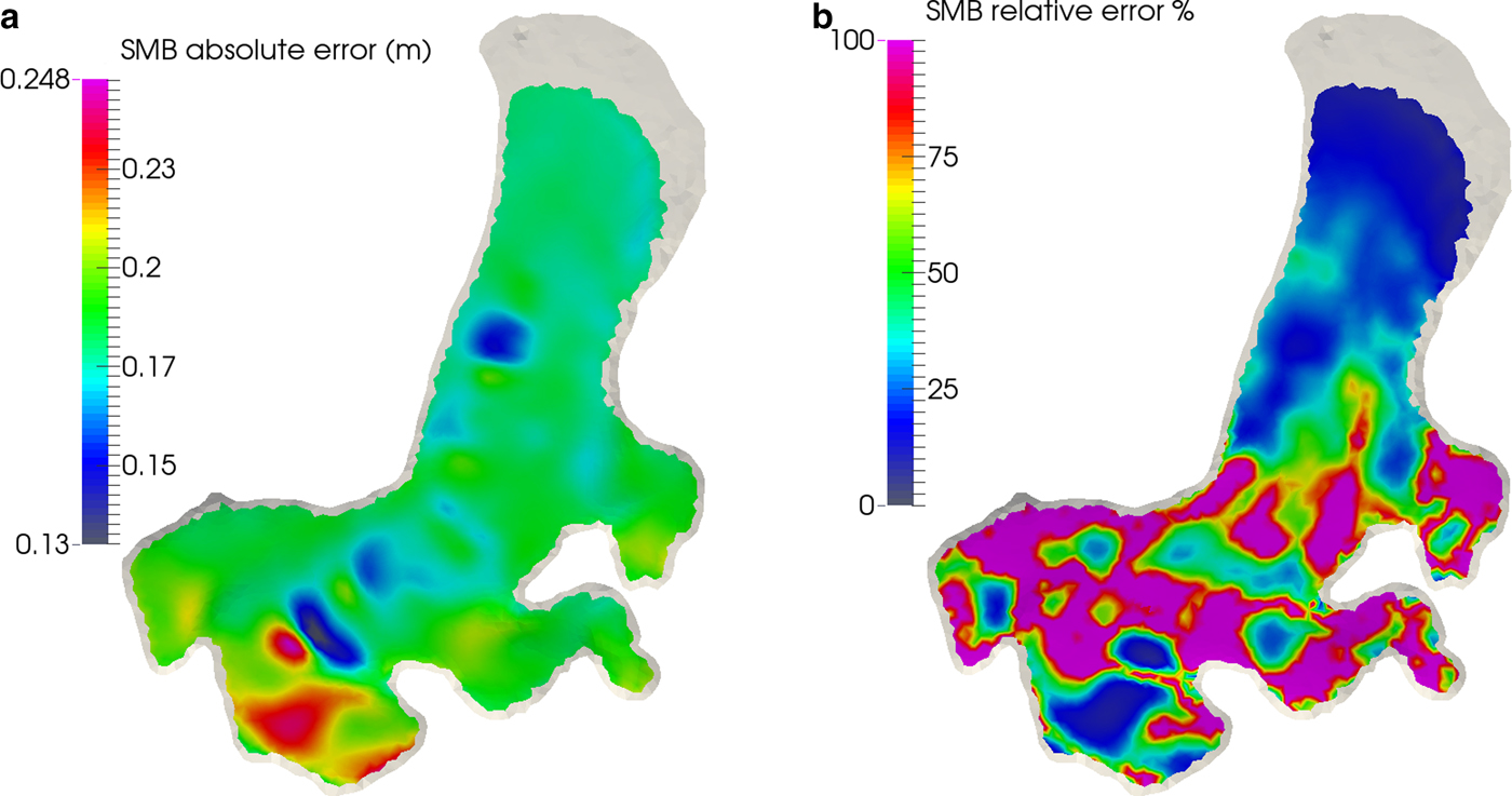
The largest absolute uncertainty in SMB has been in the area of highest accumulation and the smallest at the tongue of the glacier. However, the uncertainty proportional to the SMB is equally small in areas of highest accumulation as at the tongue. The example provided for the time interval of 1977–95 (Fig. 6) shows the distribution of the absolute uncertainty and the uncertainty proportional to the SMB. The uncertainty of SMB proportional to the total SMB reaches very high values around the areas where SMB is zero or close to zero.
The SMB error in the simualtion of 1977–95. Panel (a) shows the distribution of the absolute SMB error in meters of ice and panel (b) the SMB error relative to the SMB (%).
4.4. Contribution of ice dynamics to the surface elevation change
The part of the kinematic boundary condition [Eqn (12)] linked to glacier dynamics is equal to the negative emergence velocity. To study the relative importance of the emergence velocity,  ${\bi u}_{{\rm em}} (h_{t_1 \to t_2}, {\bi u})$, for the surface elevation change of the glacier $(\partial h_{t_1 \to t_2} /\partial t)$, we calculate the absolute values of both terms and their average ratio (Table 4). We assess the absolute values of ${\bi u}_{{\rm em}} (h_{t_1 \to t_2}, {\bi u})$ and $\partial h_{t_1 \to t_2} /\partial t$ to study the relative contribution of the terms regardless of their sign. The contribution of the emergence velocity to the surface elevation change is typically up to 2.0 m a−1 over different parts of the glacier. The greatest range was for the time period of 1977–95, with a maximum absolute value of 2.37 m a−1, whereas the smallest contribution of 1.43 m a−1 occurred in 1969–77. The total elevation change over the glacier $(\partial h_{t_1 \to t_2} /\partial t)$ is of the same order of magnitude as the elevation change caused by emergence velocity alone. The average range of $\vert\partial h_{t_1 \to t_2} /\partial t\vert$ during the different time periods reaches from 0.0 to 2.5. For a single period it is the largest in 1962–69, when the maximum absolute values was 3.02 m a−1. The narrowest range, 0.0–2.09, is seen in 1977–95.
Maximum absolute value of emergence velocity, surface elevation change and the average ratio of the absolute values at the given time intervals
Despite the maximum absolute value of  $\partial h_{t_1 \to t_2} /\partial t$ being larger than that of ${\bi u}_{{\rm em}} (h_{t_1 \to t_2}, {\bi u})$, the ratio between $\vert{\bi u}_{{\rm em}} (h_{t_1 \to t_2}, {\bi u})\vert$ and $\vert\partial h_{t_1 \to t_2} /\partial t\vert$ is typically 1.3 when averaged over the glacier. This indicates that the absolute values of emergence velocity are typically higher than the absolute values of $\partial h_{t_1 \to t_2} /\partial t$. For the 1962–69 period, the ratio was 1.6, in 1969–77 and 1977–95 it was 1.35, only falling below unity value with 0.85 for 1995–2005. This is no surprise, as ice velocities show a strong non-linear dependence on ice thickness. As both terms have negative and positive values, these ratios do not reflect the real elevation change of the glacier surface, but rather the relative importance of the glacier dynamics in shaping the glacier.
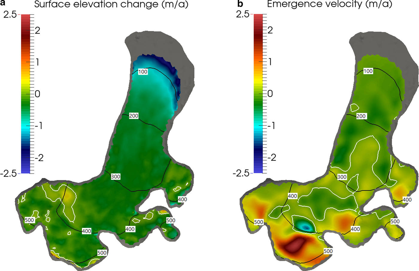
Figure 7a and b present the distribution of  $\partial h_{t_1 \to t_2} /\partial t$ and ${\bi u}_{{\rm em}} (h_{t_1 \to t_2}, {\bi u})$ for the 1977–95 period. This simulation period is selected because of the better quality of more recent DEMs and because the area with positive $\partial h_{t_1 \to t_2} /\partial t$ is still observable in 1977–95 but has completely vanished by 1995–2005. The pattern of $\partial h_{t_1 \to t_2} /\partial t$ (Fig. 7a) indicates an overall negative surface elevation change, with increasing surface elevation only in small parts of the higher reaches of the glacier. The lowering of the surface is strongest at the tongue of the glacier, up to 2.5 m a−1. In terms of emergence velocity (Fig. 7b) the glacier is rather clearly divided into areas of positive and negative emergence velocity in the upper and lower halves of the glacier. For obvious reasons, the emergence velocity is most pronounced in the fast flowing areas of the glacier and in the steepest parts of the higher elevation areas. Solving for Eqn (14) reveals that the strong ${\bi u} _{{\rm em}} (h_{t_1 \to t_2}, {\bi u})$ must be balanced by accumulation (Fig. 4c), in order to maintain the observed shape of the glacier.
Surface elevation change ( $\partial h_{t_1 \to t_2} /\partial t$, panel (a) and inverted emergence velocity ( ${\bi u}_{{\rm em}} (h_{t_1 \to t_2}, {\bi u})$, panel (b) in 1977–95. The white line is the zero contour of the variable in question. Surface elevation contours are shown in black. The emergence velocity is presented with a negative sign to reflect the related SMB.
5. DISCUSSION AND CONCLUSIONS
Based on the comparison of modelled and measured velocities, Elmer/Ice produces a good match to the observed surface velocities on ML. A velocity bias in the simulations is compensated for by adding basal sliding to the model experiments. Velocity observations show a seasonal difference in surface velocities, which strongly suggests that there actually is basal sliding at ML. In the model, basal sliding is limited to the deepest parts of the glacier, where ice thickness exceeds 120 m; this potentially affects the calculation of the mass balance by enhancing the contribution of emergence velocity. Further fine-tuning the spatial distribution and amount of basal sliding may improve the match to the observations, but the latter are too spatially limited to provide sufficient support for this approach.
The errors in the input surface DEMs are reflected by the modelled SMB. The uncertainties of the surface DEMs are significant in the past, but the DEMs get more reliable closer to present day. Also the uncertainty of the modelled SMB induced by the DEMs decreases towards present day. The error of the modelled SMB can be assessed either by looking at the absolute uncertainty (m of ice) or by evaluating the error proportional to the SMB (%). The absolute error is is largest in the accumulation area. The SMB is also highest in the accumulation area, meaning that the error proportional to SMB is not as alarming as the absolute error would suggest. The error proportional to SMB is 100% in the areas where SMB is close to zero, i.e. around the equilibrium line altitude. Thus the error proportinal to SMB is not a useful measure allover the glacier, but helps in putting the error into perspective in the areas where SMB clearly differs from zero.
The simulated SMB and ELA show similar time evolution as observed. The simulations show decreasing SMB and increasing ELA, although – as the results are based on only four time intervals – the statistical significance of the trend cannot be assessed. Compared with the glaciological stake observations averaged over the simulation periods, the model results show a more monotonic decrease/ascent in SMB/ELA. The annual mass-balance observations from 1968 to 2012 do not indicate a statistically significant decreasing trend. Nonetheless, a constantly negative mass balance is enough for a significant retreat of the glacier.
The pattern of  $\partial h_{t_1 \to t_2} /\partial t$ was much more uniform than that of a ⊥ and ${\bi u}_{{\rm em}} (h_{t_1 \to t_2}, {\bi u})$. One way to evaluate the reliability of the spatial distribution of modelled a ⊥ is to compare it with accumulation charts on Midtre Lovénbreen (Hagen and Liestøl, Reference Hagen and Liestøl1990), for the time period of 1962–69 and 1969–77, which most closely match the observation period indicated in (Hagen and Liestøl, Reference Hagen and Liestøl1990). From our simulations, we could identify a local low a ⊥ around the area that separates the southwestern tributary from the main glacier body. A similar area of low accumulation was present in Hagen and Liestøl (Reference Hagen and Liestøl1990), during a year with average precipitation. We observe a dipole of high and low a ⊥ at the southern part of the glacier, with high values above the 400 m contour, and low values below. The accumulation chart shown in Hagen and Liestøl (Reference Hagen and Liestøl1990) also shows a local minimum in the corresponding location, but does not show locally increased accumulation. Zwinger and Moore (Reference Zwinger and Moore2009) observed a similar pattern that quickly vanished in prognostic simulations, thereby indicating the possibility that a data gap in the radar sounding of the bedrock is the cause of this local deviation in diagnostic simulations.
Our results show a significant decrease in SMB in the upper reaches of the glacier for the periods 1977–95 and 1995–2005 (Fig. 5). The decrease is not visible from the glaciological stake measurements, however the observed values above the elevation of 450 m are extrapolated, and thus their representativity is questionable. Especially in 1995–2005 a ⊥ is negative at the most elevated glacier boundaries (Fig. 4). These results are in line with earlier studies that have shown accelerated thinning in the upper parts of ML (Kohler and others, Reference Kohler2007; James and others, Reference James2012). Kohler and others (Reference Kohler2007) show – based on DEMs and Lidar observations – that the thinning rate of ML in 2003–05 had doubled compared with 1962–69. Also James and others (Reference James2012) identify two different epochs of thinning: prior and after 1990s. The thinning is strongest at the high reaches of the glacier. The thinning can reflect changes in ice mass or changes in the density of firn. Kohler and others (Reference Kohler2007) estimates that density changes in ML have been negligible. James and others (Reference James2012) state that the accelerated thinning coincides with a decrease in winter accumulation, which reduces the mass input to the glacier. The submergence velocities might not be in balance with the decreased mass input, which is reflected as thinning of the upper reaches of the glacier (James and others, Reference James2012). The studies by James and others (Reference James2012) and Kohler and others (Reference Kohler2007) hypothesize that lower snow accumulation would have lead to lower albedo either by loss of fresh snow on the glacier or by increased dust transport from the bedrock areas that were previously covered by snow. Lower albedo enchances absortion of solar radiation and warming of the surface. Our result of decreased accumulation above 500 m is most likely a model response to the thinning of the glacier. We use the DEMs that indicate thinner ice at the high reaches of ML as input for Elmer/Ice. Thinner ice induces reduced flow, which we see in our inverse approach as decreased SMB. In reality the cause and consequence are the opposite: smaller accumulation and thinner ice lead to slower ice flow. The accelerated thinning has been connected to increased summer temperature and decreased winter accumulation and consequent albedo feedback. These changes affect both accumulation and ablation area, but in the snow-covered accumulation area the lowering of albedo is more important than in the ablation area, which already has a low albedo (Kohler and others, Reference Kohler2007).
We introduced a method that combines measured geodetic SMB in the form of DEMs with high-resolution glacier flow modelling to deduce the corresponding mass-balance patterns as a spatial distribution over the whole glacier. Surface DEMs often are easier to access than in-situ measurements – in particular for remote glaciers – this method could provide the possibility of augmenting remotely sensed information by modelled glacier dynamics. Since it only involves diagnostic simulations it is computationally very economical, even for glacier areas much larger than ML.
ACKNOWLEDGEMENTS
This publication is contribution number 81 of the Nordic Centre of Excellence SVALI, ‘Stability and Variations of Arctic Land Ice’, funded by the Nordic Top-level Research Initiative (TRI). Ilona Välisuo was supported by SVALI. Thomas Zwinger was supported by the Nordic Center of Excellence eSTICC (eScience Tool for Investigating Climate Change in northern high latitudes) funded by Nordforsk (grant 57001). We would like to thank the editors and the reviewers for their constructive comments on the manuscript.


 Open access