


1. Introduction
Coral reef sediments have important implications for coral reef ecosystems. These sediments can provide the community (including reefs, fleshy algae and fish) with necessary carbonate and nutrients (Dong et al. Reference Dong2023). However, with increased human activity, coral reef sediments are now even being considered as threats to the coral reef systems. Intense hydrodynamic disturbances – e.g. typhoons (Pratchett Reference Pratchett2005), blast fishing and illegal poaching of tridacna (Scales, Balmford & Manica Reference Scales, Balmford and Manica2007) – can cause suspension of sediments (Jones et al. Reference Jones, Bessell-Browne, Fisher, Klonowski and Slivkoff2016; Rogers & Ramos-Scharrón Reference Rogers and Ramos-Scharrón2022). These suspended sediments can settle directly on corals and other reef organisms, which will smother and abrade corals (Jones et al. Reference Jones, Bessell-Browne, Fisher, Klonowski and Slivkoff2016; Rogers & Ramos-Scharrón Reference Rogers and Ramos-Scharrón2022). The suspended sediments can also reduce the coral photosynthesis by blocking light. The velocity of settling has been shown to influence the attachment and survival rates of coral larvae (Babcock & Smith Reference Babcock and Smith2002; Rogers & Ramos-Scharrón Reference Rogers and Ramos-Scharrón2022). Understanding of settling motion and having predictive capacity for the settling velocity are critical in terms of helping to protect coral reef systems from those threats and restore the ecosystems effectively.
The settling motion has been explored in detail for a circular disk and a sphere with uniform shape but not for coral grains. For a circular disk, three regimes of settling trajectory were classified in Field et al. (Reference Field, Klaus, Moore and Nori1997), namely, fluttering, chaotic and tumbling. It has been demonstrated that the settling trajectory is highly dependent on the object geometry (Maiklem Reference Maiklem1968). For a sphere, more fruitful regimes were observed (Raaghav, Poelma & Breugem Reference Raaghav, Poelma and Breugem2022). In reality, the presence of biological structure of coral grains makes their geometry more complicated than the disk and sphere (Wang et al. Reference Wang, Wu, Cui, Zhu and Wang2020), which increases the complexity of settling motion (de Kruijf et al. Reference de Kruijf, Slootman, de Boer and Reijmer2021). Understanding the settling motion of coral grains is one of motivations of this study.
In the settling motion, when the effective force (gravity minus buoyancy) is equal to the drag force on the particle in the vertical direction (over the depth), the particle will fall with an equilibrium settling velocity  $\omega$. Different empirical models have been proposed for predicting the setting velocity for particles from different sources. For natural quartz, the model in Dietrich (Reference Dietrich1982) established the relationship of dimensionless velocity $W^\ast$ with the non-dimensional particle diameter $D^\ast$ ( $W^\ast$ and $D^\ast$ are parameters non-dimensionalised by Reynolds number (Re) and drag coefficient). This relationship was then extended to carbonate grains in Li et al. (Reference Li, Yu, Gao and Flemming2020). This is different from the semi-empirical model proposed in Riazi et al. (Reference Riazi, Vila-Concejo, Salles and Türker2020) for carbonate sediments, in which the settling velocity is a function of $S$ (the specific gravity of the particle), $C_{D}$ (the drag coefficient), $S_{f}$ (the Corey shape factor) and $D_{n}$ (the nominal diameter). In comparison to these models, the model in Alcerreca, Silva & Mendoza (Reference Alcerreca, Silva and Mendoza2013) simply established the relationship between $Re$ and $D^\ast$ ( $\omega$ is embedded in $Re$).
There is also a range of models that can be used to estimate the drag coefficient  $C_{D}$. First, the drag coefficient of a coral grain can be estimated through direct measurements of settling velocity, densities of coral grain and fluid, and the geometry of the grain. The drag coefficient can also be evaluated through the empirical model of Riazi et al. (Reference Riazi, Vila-Concejo, Salles and Türker2020), which links $C_{D}$ to the nominal diameter and the kinematic viscosity of fluid. Finally, the drag coefficient can be predicted by the model of Wang et al. (Reference Wang, Zhou, Wu and Yang2018), in which $C_{D}$ is a function of Reynolds number and the Corey shape factor.
Although different models of settling velocity and drag coefficient have been developed in literature, grain shape parameters in these models still rely on some kind of approximation of spherical or tri-axial geometries. These approximated parameters sometimes are not that representative to the real geometry of coral grains. Since both settling velocity and drag coefficient are highly dependent on the grain geometry (Maiklem Reference Maiklem1968), applying these models to real systems can be problematic if the targeted grains are very different from the unknown particles used in the validation of the empirical models. This highlights the importance of using coral grains with fully categorised, quantified geometry to validate existing empirical models. In such a way, the applicable range of validated/modified models is well defined.
There is a range of approaches used to classify coral reef grains. For simplicity of classification, the coral grains were normally simplified into an ellipsoid (Wadell Reference Wadell1932; Krumbein Reference Krumbein1941; Oakey et al. Reference Oakey, Green, Carling, Lee, Sear and Warburton2005). The long, medium and short axes of the ellipsoid ( $D_{l}$, $D_{m}$ and $D_{s}$ were found to be important dimensions in the classification. Based on the dimensionless variables $D_{m}/D_{l}$ and $D_{s}/D_{m}$, coral grains were classified into four sub-populations, namely, discoid, blade, rod and spheroid (Zingg Reference Zingg1935). In contrast, based on a combined parameter set ( $D_{m}/D_{l}$, $D_{s}/D_{l}$ and $(D_{l}-D_{m})/(D_{l}-D_{s})$), the sediments can be categorised into four types: platy, bladed, elongated and compact (Sneed & Folk Reference Sneed and Folk1958). In comparison to these two classification methods based on the simplification of ellipsoid, there is another approach proposed in Wang et al. (Reference Wang, Wu, Cui, Zhu and Wang2020). This approach was established based on both first- and second-order shape descriptors.
In the light of existing work, this paper aims to investigate the settling motion of 222 coral grains from the South China Sea, with three specific objectives: (1) categorise these coral grains; (2) classify the settling trajectory of coral grains; (3) validate and extend existing models for predicting settling velocity and drag coefficient.
2. Methodology
2.1. Geometric parameters
There are three orders of the scale for describing the shapes of irregular particles (figure 1): form, roughness and surface texture (Griffiths Reference Griffiths1967; Barrett Reference Barrett1980). However, limited by the availability of measuring equipment, most studies on shape quantification have focused on the first and second orders of scale. In the first order of scale, form is the fundamental descriptor of the three-dimensional spatial distribution of a particle in space. As shown in figure 2, the lengths of three axes (i.e. long axis  $D_{l}$, intermediate axis $D_{m}$, and short axis $D_{s}$) of the ellipsoid can characterise the three-dimensional spatial distribution of the particle (Barrett Reference Barrett1980; Oakey et al. Reference Oakey, Green, Carling, Lee, Sear and Warburton2005; Blott & Pye Reference Blott and Pye2008; Heilbronner & Barrett Reference Heilbronner and Barrett2013). Based on these dimensions, several dimensionless parameters are used to describe the form of the particles, such as the flatness $D_{s}/D_{m}$ (Blott & Pye Reference Blott and Pye2008), elongation $D_{m}/D_l$ (Lüttig Reference Lüttig1956), and equancy ${D_{s}}/{D_{l}}$ (Illenberger Reference Illenberger1991). Meanwhile, Wadell (Reference Wadell1932, Reference Wadell1933) and Corey et al. (Reference Corey, Albertson, Fults, Rollins, Gardner, Klinger and Bock1949) defined the nominal diameter and the Corey shape factor, respectively, for the non-spherical grains as
 $$\begin{gather} {D_n} = \sqrt[3] {{D_l}{D_m}{D_s}} , \end{gather}$$
 $$\begin{gather}S_{f} = \frac{{{D_s}}}{{\sqrt {{D_l}{D_m}} }} . \end{gather}$$
Figure 1. Shape descriptors of three orders for a coral grain.
In the second order of scale, roundness characterises the smoothness of the particles. Establishing the shape parameters at the roundness scale is usually achieved by quantifying the difference of the grain shape from the spherical shape (see figure 3) with the sphericity  $\phi$, a ratio between surface area $A_{eq,\,sph}$ of a sphere and that of the particle, $A_p$ (the sphere has the same volume as the particle). However, the shape of coral sand particles is complex at the roundness scale (figure 1) due to the deposition processes in coral islands and the presence of skeletal structures (Slootman et al. Reference Slootman, de Kruijf, Glatz, Eggenhuisen, Zühlke and Reijmer2023). These parameters may not be sufficient to describe the geometry of coral particles. To address this, a new shape parameter $\psi$ was proposed in Wang et al. (Reference Wang, Zhou, Wu and Yang2018) for describing the highly irregular grains, which is defined as
 \begin{equation} \psi = \frac{\phi }{X},\quad\phi = \frac{{{A_{eq,\,sph}}}}{{{A_p}}},\quad X = \frac{{{P_{p,\,max }}}}{{{P_{eq}}}} , \end{equation}
where  $\phi$ is sphericity, ${A_{eq,\,sph}} = {\rm \pi}{( {{D_{eq,\,sph}}} )^2}$ is the surface area of the volume-equivalent sphere, ${D_{eq,\,sph}} = {( {({6}/{{\rm \pi} }){V_p}} )^{1/3}}$ is the diameter of the volume-equivalent sphere, $V_{P}$ is the particle volume, ${A_p}$ is the surface area (which is calculated as ${A_p} \approx A_{ell} = {\rm \pi}[(D_lD_m)^\kappa + (D_lD_s)^\kappa + (D_mD_s)^\kappa /{3}]^{{1}/{\kappa }}$, with $\kappa = 1.6075$), ${A_{ell}}$ is the surface area of the irregular particles under the tri-axial orthogonal system of the ellipsoid (figure 2), ${P_{p,\,max}}$ is the perimeter of the maximum projection area of the particle, and ${P_{eq}}$ is the perimeter of a circle with the same maximum projection area as the particle.

Figure 2. Tri-axial orthogonal system of the ellipsoid simplification of a real coral grain.

Figure 3. Diagram of shape descriptors reported in Wang et al. (Reference Wang, Meng, Wei, Chen, Yan and Zhang2019).
The original classification method based on the first-order shape descriptors (figure 4) was unable to describe the particular shape of the coral sand grains (see figure 1) due to the complexity of the particle shape. Wang et al. (Reference Wang, Meng, Wei, Chen, Yan and Zhang2019) summarised a series of the first-order and second-order shape descriptors from the studies of Mora & Kwan (Reference Mora and Kwan2000), Kwan, Mora & Chan (Reference Kwan, Mora and Chan1999) and Hentschel & Page (Reference Hentschel and Page2003) (see table 1). Wang et al. (Reference Wang, Meng, Wei, Chen, Yan and Zhang2019) then classified coral grains into dendrites, rods, flakes and blocks based on both first- and second-order shape descriptors (tables 2 and 3). These descriptors based on three dimensions were determined with multi-photographs taken from different angles of view.

Figure 4. Irregular particle classification based on the first-order shape descriptors: (a) classification diagram from Zingg (Reference Zingg1935), and (b) equant–oblate–prolate ternary classification diagram by Sneed & Folk (Reference Sneed and Folk1958).
Table 1. Two-dimensional (2-D) and three-dimensional (3-D) first-order shape descriptors.

Table 2. Particle shape parameters in Wang et al. (Reference Wang, Meng, Wei, Chen, Yan and Zhang2019).

Table 3. Classification criteria for calcium sand with various shapes in Wang et al. (Reference Wang, Meng, Wei, Chen, Yan and Zhang2019).

2.2. Predictive models of drag coefficient and settling velocity
2.2.1. Models for estimating  $C_D$
$C_D$

(i) Model I_D (direct measurement)
When the effective weight is equal to the drag force of particle in the vertical direction, the particle falls with terminal settling velocity. At this stage, the momentum balance in the vertical direction (over depth) can be expressed as
(2.4)where\begin{equation} ( {{\rho _s} - {\rho} } )gV = \tfrac{1}{2}\rho {C_D}{A_P}{\omega ^2} , \end{equation}$\rho _{s}$ and $\rho$ are the densities of coral grain and fluid, respectively, $g$ is the gravitational acceleration, $V$ is the volume of the coral grain, ${C}_{D}$ is the drag coefficient, $A_{P}$ is the maximum projected area of the particle, and $\omega$ is the particle settling velocity. Equation (2.4) can be rewritten in the form
(2.5)where\begin{equation} {C_D} = 2\,\frac{{( {S - 1} )g}}{{{\omega ^2}}}\,\frac{V}{{{A_P}}} , \end{equation}$S = {\rho _{s}}/\rho$ is the specific gravity of the particle. The drag coefficient can be determined by measuring all the quantities on the right-hand side of (2.5).(ii) Model II_D (Riazi et al. Reference Riazi, Vila-Concejo, Salles and Türker2020)
Based on the data of Smith & Cheung (Reference Smith and Cheung2002), Riazi et al. (Reference Riazi, Vila-Concejo, Salles and Türker2020) used a genetic algorithm (Riazi & Türker Reference Riazi and Türker2018) to obtain an expression for
$C_{D}$ of coral grains:
(2.6)where\begin{equation} {C_D} = {\left( {\frac{{9.50 \times \nu }}{{D_n^{1.5} \times {g^{0.5}}}} + 0.76} \right)^{2.92}} + {\left( {\frac{{20.47 \times \nu }}{{D_n^{1.5} \times {g^{0.5}}}} + 1.02} \right)^{ - 48.15}} , \end{equation}$\nu$ is the kinematic viscosity of the fluid.(iii) Model III_D (Wang et al. Reference Wang, Zhou, Wu and Yang2018)
Wang et al. (Reference Wang, Zhou, Wu and Yang2018) obtained the relationship between drag coefficient and Reynolds number based on experimental data of 521 calcareous sand particles, which is expressed by
(2.7)\begin{equation} \left.\begin{gathered} {C_D} = 0.945\,\frac{{{C_{D,\,sph}}}}{{{\psi ^{f( {{Re} } )}}}}\,{{Re} ^{ - 0.01}} ,\\ {{C_{D,\,sph}} = \frac{{24}}{{Re}}\left( {1 + 0.15\,Re^{0.687}} \right) + 0.42\left/ \left( {1 + \frac{{42\,500}}{{Re^{1.16}}}} \right)\right.} ,\\ f( {{Re} } ) = 0.641\,{{Re} ^{0.153}} ,\\ Re = \frac{{\rho \omega D_n}}{\mu } . \end{gathered}\right\} \end{equation}


2.2.2. Models for predicting setting velocity
(i) Model I_V (Riazi et al. Reference Riazi, Vila-Concejo, Salles and Türker2020)
Using an approximation of ellipsoids to natural particles, Riazi et al. (Reference Riazi, Vila-Concejo, Salles and Türker2020) found that the ratio of the volume
$V$ to the projected area ${A_{P}}$ is a function of $S_{f}$ and ${D_{n}}$, with the relationship
(2.8)where\begin{equation} \frac{V}{{{A_P}}} = \alpha\,\frac{2}{3}\,(S_f)^{(2/3)}{D_n} , \end{equation}$\alpha = 0.55$ based on their experimental data. The derivation of (2.8) was based on extensive observations that natural particles will adjust themselves into a state where the maximum projected area (${A_p} = {{{\rm \pi} {D_l}{D_m}}}/{4}$) is normal to the settling direction, regardless of the orientation of the particle being realised into fluid (Dietrich Reference Dietrich1982; Alldredge & Gotschalk Reference Alldredge and Gotschalk1988; Khatmullina & Isachenko Reference Khatmullina and Isachenko2017; Riazi & Türker Reference Riazi and Türker2019). Equation (2.8) was validated here by measuring variables on both sides of this equation, which gives measured values of $\alpha$. The root mean square error (RMSE) between the measured values of $\alpha$ and 0.55 determined by Riazi et al. (Reference Riazi, Vila-Concejo, Salles and Türker2020) is $32.5\,\%$ for our 222 coral grains, which supports the applicability of this equation to the present study.
Equation (2.4) can be rewritten as
(2.9)Combining (2.8) with (2.9) gives\begin{equation} {\omega ^2} = 2\,\frac{{( {S - 1} )g}}{{{C_D}}}\,\frac{V}{{{A_P}}} . \end{equation}(2.10)Note that\begin{equation} {\omega ^2} = \alpha\,\frac{4}{3}\,\frac{{(S - 1)g}}{{{C_D}}}\,S_f^{{2}/{3}}{D_n} . \end{equation}$C_D$ is unknown in (2.10). In practice, this model needs to be combined with the drag model II_D to provide a closed-form solution for both the velocity and the drag coefficient.(ii) Model II_V (Dietrich Reference Dietrich1982)
Many researchers (Rouse et al. Reference Rouse1938; Schulz, Wilde & Albertson Reference Schulz, Wilde and Albertson1954; Dietrich Reference Dietrich1982) have described the settling velocity in a dimensionless form of
$W^\ast$ as
(2.11)By analogy, the particle diameter was also expressed as\begin{equation} W^* = {\left[ {\left( {\frac{4}{3}} \right)\frac{{{Re} }}{{C_{D,\,sph}}}} \right]^{{-}1/3}} = \omega {\left[ {\nu g( {S - 1} )} \right]^{{-}1/3}}. \end{equation}(2.12)Dietrich (Reference Dietrich1982) collected a large amount of experimental data of natural silicate particles and proposed a model of settling velocity based on particle shape characteristics (particle size\begin{equation} D^* ={\left[ {\frac{3}{4}\,{{( {{Re} } )}^2}\,{C_{D,\,sph}}} \right]^{1/3}} = D\left[ {{{\left( {\frac{{{1}}}{\nu }} \right)}^2}g( {S - 1} )} \right]^{1/3} . \end{equation}$D^\ast$, particle shape $S_f$, particle roughness $P$):
(2.13)\begin{equation} \left.\begin{gathered} {W^*} = {R_3}{10^{{R_1} + {R_2}}},\\ {R_1} ={-}3.76715 + 1.92944\log D^* - 0.09815{(\log D^*)^2} \\ {}- 0.00575{(\log D^*)^3} + 0.00056{(\log D^*)^4} ,\\ {R_2} = \log \left(1 - \frac{{1 - S_{f}}}{{0.85}}\right) - {(1 - S_f)^{2.3}}\tanh (\log D^* - 4.6)\\ {}+ 0.3(0.5 - S_f){(1 - S_{f})^2}(\log D^* - 4.6) ,\\ {R_3} = {\left[ {0.65 - \frac{{S_f}}{{2.83}}\tanh \left( {\log D^* -4.6} \right)} \right]^{1 + (3.5 - P)}} - 4.6 .\\ \end{gathered}\right\}\end{equation}(iii) Model III_V (Li et al. Reference Li, Yu, Gao and Flemming2020)
Li et al. (Reference Li, Yu, Gao and Flemming2020) modified the model of Dietrich (Reference Dietrich1982) and extended it to 320 sets of platy shell fragments, with the simplified form
(2.14a)where$$\begin{gather} W^{*} = {10^{a\log (D^*) + b\log (S_f)+c}}, \end{gather}$$$a=0.416651$, $b=0.5316$ and $c=0.3891$.(iv) Model IV_V (Alcerreca et al. Reference Alcerreca, Silva and Mendoza2013)
To have a quick prediction tool, Alcerreca et al. (Reference Alcerreca, Silva and Mendoza2013) developed a model of settling velocity based on 1557 calcareous sand grains as
(2.15)Equation (2.15) can be rewritten in the form of settling velocity as\begin{equation} Re = {\left( {\sqrt {22 + 1.13D^{*^2}} - 4.67} \right)^{3/2}} . \end{equation}(2.16)\begin{equation} \omega = {{Re}}\,\frac{v}{{{D_n}}} = \frac{v}{{{D_n}}}{\left( {\sqrt {22 + 1.13{D^*}^2} - 4.67} \right)^{3/2}} . \end{equation}


2.2.3. Performance metric
In this paper, the RMSE is used as a metric for evaluating the performance of different models:
 \begin{equation} {\rm RMSE(\%)} = {\left( {\frac{{\sum {{{({\rm{Estimated}} - {\rm{Measured}})}^2}} }}{{\sum {{{\left( {{\rm{Measured}}} \right)}^2}} }}} \right)^{0.5}} \times 100 . \end{equation}
A smaller RMSE value indicates better model performance.
2.3. Experimental set-up
A series of experiments was conducted to study the settling motion of the coral grains at the Hydraulic Engineering Laboratory, Changsha University of Science and Technology, China. A Plexiglas tank (0.3 m long, 0.3 m wide and 0.8 m deep) was designed for the test, and the tank was filled with water at temperature  $24 \pm 3\,^{\circ }\textrm {C}$, density $\rho = 1000\ \textrm {kg}\ \textrm {m}^{-3}$ and dynamic viscosity $\mu =1.247 \times 10^{-3}\ \textrm {Pa}\ \textrm {s}$. The water depth in the tank was maintained at 0.80 m in the experiments. Since there are pores in the dry coral grains, bubbles will be generated from the particles when they settle down. To avoid the influence of bubbles on the settling motion, dry coral grains were immersed in the water for 24 h before testing. There was a minimum relaxation time of 5 min between each experiment, to ensure the water is truly still in the tank before the next run. The coral grain was cleaned from the bottom after each experiment such that it will not occupy the volume in the tank to increase the water depth.
Figure 5 shows the experimental set-up. The background water in the tank was illuminated using a continuous laser sheet, and the light source had wavelength 532 nm (Laserwave, G2000). Black curtains were placed around the tank to eliminate wall reflections of light. The settling motion of a coral grain in the water was recorded with two high-speed cameras (FASTCAM Mini UX100 and MEMRECAM HX-7S) in two orthogonal directions (see figure 5a). Both cameras were equipped with AF50 mmf/1.8DI camera lenses (Nikon, Japan) and had resolution  $1024 \times 1024$ pixels. Raw images were recorded at 50 Hz, which was controlled by computer image capture software (Photron Motion Tools). The camera was calibrated by the MATLAB toolbox ‘camera calibrator’.

Figure 5. (a) Image of experimental set-up for monitoring the settling motion of coral grains by a charge-coupled device (CCD) camera (in the  $X$ and $Y$ directions, respectively). (b) Sketch of the acrylic tank in (a). The volume ( $30\ \textrm {cm} \times 30\ \textrm {cm} \times 25\ \textrm {cm}$) monitored by the two cameras is shaded in grey. A coral sand particle was released from the point $O$ without initial velocity.
The volume of interest was a cuboid measuring  $0.30\ \textrm {m} \times 0.30\ \textrm {m}\times 0.25\ \textrm {m}$ (see figure 5b). To reconstruct the settling process of the coral grains, the algorithm for particle filtering was implemented in MATLAB, for which the regionprops library was used. The positions of a coral grain in settling were tracked (in MATLAB) from images taken at every moment (figure 6). After the particle had undergone the initial acceleration phase (Heisinger, Newton & Kanso Reference Heisinger, Newton and Kanso2014), it entered the vertical force equilibrium phase (see figure 7). Each particle was tested five times. The terminal settling velocity of the particle was calculated by averaging velocities of the five repeated runs. The relative error (2.18) for all the cases in the present work is less than 5 %, demonstrating the repeatability of experiments (see table 4):
 \begin{equation} {Q_i} = \frac{{\sum\limits_{j = 1}^5 {\left| {\dfrac{{{\omega _j} - \omega }}{\omega }} \right|} }}{5} \times 100\,\% . \end{equation}
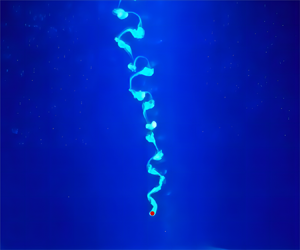
Figure 6. An example of the settling trajectory of a particle tracked by the particle filtering algorithm based on MATLAB. White dots in each image represent the historical particle positions, and each dot was processed from one image. The green dot in each image represents the particle position at the moment.

Figure 7. The temporal evolution of the particle velocity in the settling motion for a coral grain with  $D_{n}=2.63$ mm.
Table 4. Relative error of repeated tests.

The lengths of the long, middle and short axes ( ${D_{l}}$, ${D_{m}}$ and ${D_{s}}$, respectively) were measured by the following procedure. Specifically, following fluorescence microscopy (OLYMPUS BX43), the grain was first placed on the microscope stage, and a photograph was taken of it. After this, the grain was rotated about the axis along which the distance across the particle is visually longest. Then another photograph was taken of this newly positioned grain. Repeating this process produces multi-angle photographs. In each photograph, the length and width of the grain can be determined through two approaches in OpenCV (Zingg Reference Zingg1935; Wang et al. Reference Wang, Zhou, Wu and Yang2018) as illustrated in figure 8. Specifically, the length and width can be determined through the minimum outer rectangle measurement (figure 8a) or the best fitting ellipse measurement (figure 8b). The largest length among these photographs was defined as the long axis length ${D_{l}}$. Among widths in these photographs, the longest one was defined as the middle axis length ${D_{m}}$, whereas the shortest one was considered as the short axis length ${D_{s}}$.

Figure 8. Determination of three ellipsoid axes based on image recognition. (a) Approach of the best-fit ellipse of ImageJ from Wang et al. (Reference Wang, Zhou, Wu and Yang2018). (b) Approach of the minimum bounding rectangle from Chen et al. (Reference Chen, Yao, Jiang, Wu, Deng, Long and Bian2022).
A total of 222 experiments were conducted to investigate the settling motion of coral grains. The experimental particles conform to the coral and gastropod grains described in de Kruijf et al. (Reference de Kruijf, Slootman, de Boer and Reijmer2021). Coral grains were sieved into 10 groups using 10 sieve shakers with sieve numbers ranging from 0.25 mm to 5 mm. To measure the density of coral grains, a set of coral grains with total mass 100 g was picked from one of groups. The volume of this set of grains was measured through the drainage method. In such a way, the density for this set of grains was determined. Repeating this process for each group of sieved coral grains yielded individual densities. Averaging these 10 densities gives the real density ( $2700\ \textrm {kg}\ \textrm {m}^{-3}$) for these mixed coral grains.
In our experiments, the coral grains classified by Zingg (Reference Zingg1935) and Wang et al. (Reference Wang, Meng, Wei, Chen, Yan and Zhang2019) are both mapped out in the parameter space defined by Sneed & Folk (Reference Sneed and Folk1958) in figure 9. Wide ranges of  $D_{n}$ ( $1.47\unicode{x2013} 5.23$ mm) and $S_{f}$ ( $0.22\unicode{x2013} 0.99$) were examined (see figures 10 and 11), which covered the nominal diameter range of Hongbing, Sun & Cheng (Reference Hongbing, Sun and Cheng2006) for the Nansha Islands. The distribution of the range of shape coefficients for different shapes of coral sand particles is shown in figure 11.

Figure 9. (a) Mapping coral grains classified by the method of Sneed & Folk (Reference Sneed and Folk1958) into the parameter space defined by Zingg (Reference Zingg1935). (b) Mapping coral grains classified by the method of Wang et al. (Reference Wang, Meng, Wei, Chen, Yan and Zhang2019) into the parameter space defined by Zingg (Reference Zingg1935).

Figure 10. Distribution of nominal diameter  $D_{n}$ for a total of $n=222$ grains. Here, $\mu$ is the mean, and $\sigma$ is the standard deviation.

Figure 11. Proportion of each type of coral grain within each interval of shape factor  $S_f$. A total of 222 coral grains were classified by the methods of (a) Sneed & Folk (Reference Sneed and Folk1958), (b) Zingg (Reference Zingg1935), and (c) Wang et al. (Reference Wang, Meng, Wei, Chen, Yan and Zhang2019).
Note that all the symbols used in this paper are summarised in the Appendix.
3. Results
3.1. Classification of descent regimes of coral grains
With laboratory experiments, three regimes of settling motion are classified for coral grains based on the reconstructed three-dimensional settling trajectory, the spiral radius  $r$ defined as
 \begin{equation} r = \sqrt {{X^2} + {Y^2}}, \end{equation}
and the spectrum of settling velocity (see figure 12). The regime classification is based on the fully developed motion for which the settling velocity reaches an equilibrium state. The three regimes, namely, fluttering, tumbling and chaotic, are similar to those identified for spherical (Raaghav et al. Reference Raaghav, Poelma and Breugem2022) and disk-like particles (Field et al. Reference Field, Klaus, Moore and Nori1997).

Figure 12. Regime classification of settling trajectory. (a,d,g,j) Reconstructed three-dimensional trajectory with the projections of trajectory in different planes, with  $D^*=49, 72, 90, 75$, $W^{*}=6.5, 9.6, 7.2, 4.0$ and $S_{f}=0.84, 0.74, 0.40, 0.22$. (b,e,h,k) Variation of normalised spiral radius with time. (c,f,i,l) Spectra of velocities in the $x$ and $y$ directions. Fluttering, tumbling and chaotic regimes are characterised by a spiral trajectory in (a), sideways drifting in (d,g), and a chaotic trajectory in (j), respectively.
The fluttering regime is characterised by a three-dimensional spiral trajectory about a vertical axis (see figure 12a). The projection of the trajectory in the  $x\unicode{x2013} y$ plane forms an elliptical path (figure 12a). This elliptical path is further demonstrated by figure 12(b), where the normalised spiral radius $r/r_{max}$ first increases and then decreases with time, with values of $r/r_{max}$ equal at two ends of $t/t_{max}$ (figure 12b). The spiral forms oscillations in both the $x\unicode{x2013} z$ and $y\unicode{x2013} z$ planes, with wavelength approximately 120 $D_{n}$ (figure 12a). The oscillations in these two planes are indicated by two dominant peaks ( $\,f = 0.58, 0.78$ Hz) respectively in the spectra of velocities on the $x$ and $y$ axes (see figure 12c).
In the tumbling regime, a grain drifts sideways when settling downwards, as shown by the three-dimensional trajectory in figures 12(d,g). The projection of the trajectory in any plane displays a path extending in a particular direction (figures 12d,g). The tumbling regime has two sub-regimes, i.e. steady drifting regime and oscillatory drifting regime. The grain purely drifts in the steady drifting regime (figure 12d), in contrast to the oscillatory drifting regime where the drifting is accompanied by small-scale oscillations with wavelength 10 $D_{n}$ (figure 12g). Consistently, the spiral radius shows a linear variation with time in the steady drifting regime (figure 12e), whereas periodic fluctuations are superimposed on the increase of $r/r_{max}$ in the oscillatory drifting regime (figure 12h). The drifting behaviour in the tumbling regime is indicated by dominant peaks at $f \approx 0$ Hz (figures 12f,i). For the oscillatory drifting regime, another dominant peak appears at $f = 5$ Hz in the $x$-velocity spectrum but not in the $y$-velocity spectrum (figure 12i). The oscillation occurs on only one axis (figure 12g), which distinguishes it from the fluttering regime where the spiral creates oscillations on both $x$ and $y$ axes (see figure 12a).
The chaotic regime is characterised by a random combination of drifting and spiral (figure 12j) . The spiral radius fluctuates irregularly with time (figure 12k). The chaotic nature of this regime is indicated by multiple peaks spanning a broad range 1–10 Hz in the velocity spectra (figure 12l).
The settling regime depends on the geometry of coral grains. To demonstrate this, the coral grains are classified based on three existing approaches in figure 13.

Figure 13. Probabilities of occurrence of fluttering (F), chaotic (C), and tumbling (T) regimes for different shapes of coral grains classified based on three previous approaches. The fifth column in (a,c,e) represents the average percentage of each regime across four different shapes of classified grains. The probability of occurrence of each regime differs between different types of grains, demonstrating the dependence of descent regimes on the geometry of grains.
First, coral grains can be classified into compact, bladed, platy and elongated by following Sneed & Folk (Reference Sneed and Folk1958) (figures 13a,b). For bladed and elongated grains, the probabilities of occurrence of the fluttering, chaotic and tumbling regimes are close to each other (figure 13a). Distinctly, for the platy grains, only chaotic and tumbling regimes are observed, with occurrence probabilities  $60\,\%$ and $40\,\%$, respectively (figure 13a). The highest occurrence probability (39 %) of the fluttering regime appears for compact grains.
Second, for the classification method of Zingg (Reference Zingg1935), the probabilities of occurrence of the fluttering, chaotic and tumbling regimes approach each other for the discoid and spheroid grains (figures 13c,d). For the blade grains, the occurrence probability of the chaotic regime is up to  ${\sim }60\,\%$ (figure 13c). The rod grains have highest occurrence probabilities for both the fluttering and tumbling regimes (figure 13c).
Finally, when following the method of Wang et al. (Reference Wang, Wu, Cui, Zhu and Wang2020), it is found that the occurrence probability of the chaotic regime is approximately  $71\,\%$ for flake grains, with $21\,\%$ and $8\,\%$ for the fluttering and tumbling regimes, respectively (figures 13e,f). In contrast, the highest probability is $56\,\%$ for the fluttering regime of the dendrite grains. For the rod and block grains, the occurrence probabilities of tumbling regimes are significantly increased relative to the other two types of grains (figure 13e).
The averages of probabilities of occurrence of the tumbling, chaotic and fluttering regimes across the four different types of grains are approximately  $26\,\%$, $42\,\%$ and $32\,\%$, respectively, regardless of the classification methods applied (see figures 13a,c,e). This suggests that if one randomly picks up one coral grain, then the probabilities of occurrence of the three regimes are approximately $26\,\%$, $42\,\%$ and $32\,\%$, respectively.
Whilst the dendrite grains have the highest occurrence probability ( $56\,\%$) of the fluttering regime, the flake grains have the highest probability ( $71\,\%$) of occurrence of the chaotic regime. The tumbling regime occurs most likely for platy grains ( $36\,\%$). Clearly, these are higher than the averaged probabilities ( $32\,\%$, $42\,\%$, $26\,\%$) shown above. This means that classifying the grains based on existing methods to some extent can help to improve our predictive accuracy of descent regimes for a given coral grain.
3.2. Prediction of settling velocity and drag coefficient
In this subsection, the applicability of existing empirical models for predicting settling velocity  $W^{*}$ and drag coefficient $C_{D}$ is demonstrated. Whilst the models of settling velocity are based mostly on dimensionless diameter $D^{*}$ and the Corey shape factor $S_{f}$, the models of drag coefficient are based primarily on the Reynolds number $Re$ and shape parameters. Therefore, to validate these models in predicting the settling velocity and the drag coefficient, we start by demonstrating the dependencies of $W^{*}$ on $D^{*}$ and $S_{f}$, and $C_{D}$ on $Re$ and $S_{f}$, with experimental measurements in figure 14, which provides a physical basis for applying these models.

Figure 14. (a) The variation of settling velocity with the dimensionless diameter and shape factor. (b) The variation of drag coefficient with the particle Reynolds number and shape factor. The result from the model of Wang et al. (Reference Wang, Zhou, Wu and Yang2018) is incorporated in (b) for comparison. In both (a,b), regimes are differentiated by different symbols. Whilst the dependence of settling velocity on  $W^{*}$ and $S_{f}$ is demonstrated in (a), the relationship of drag coefficient with $Re$ and $S_{f}$ is confirmed in (b).
Figure 14(a) shows that the settling velocity generally increases with  $D^{*}$ and $S_{f}$. For the same $D^{*}$, for instance $D^{*} = 80$, with increasing $S_{f}$ from 0 to 1, the settling velocity can even vary from 4 to 10 by a factor of 2. This suggests that the settling velocity increases as the shape of a particle increasingly approaches the sphere. This velocity becomes less sensitive to the particle shape with increasing $D^{*}$. The data points in the chaotic regime set the lower limit of $W^{*}$ when $D^{*} < 80$ and $S_{f} \rightarrow 0$. This implies that a non-spherical coral grain in the chaotic regime generally has lower settling velocity relative to that in the other two regimes when $D^{*} < 80$.
In contrast, the drag coefficient generally decreases with  $Re$ and $S_{f}$ (figure 14b). The measured data are in agreement with those predicted by model III_D of Wang et al. (Reference Wang, Zhou, Wu and Yang2018). The decreasing trend of $C_{D}$ with $Re$ is consistent with previous work about flow past a stationary plate and sphere (e.g. Almedeij Reference Almedeij2008; Duan, He & Duan Reference Duan, He and Duan2015) in the range $Re \sim O(10^2\unicode{x2013} 10^3)$. There are some data points deviating from this predicted curve, which are mostly from the chaotic regime and at two ends of $S_{f}$. This is expected since there are complex self-rotations superimposed on the vertical settling motion (observed in experiments) for these deviated data points, which may suppress the shear layer separation from the grain surface and hence reduce the form drag of the grain.
With the demonstrated dependencies of  $W^{*}$ and $C_{D}$ above, we now can validate the existing models by presenting comparisons between the measurements and predictions of velocity and drag coefficient in figure 15. In the comparisons, we retain the velocity forms including $W^{*}$, $\omega$ and $Re$, as presented originally in these velocity models.

Figure 15. Comparison between the measured and predicted settling velocity in (a–d) and drag coefficient in (e). There is a large difference in the prediction accuracy among different velocity and drag models. (a) Model I_V (Riazi et al. Reference Riazi, Vila-Concejo, Salles and Türker2020). (b) Model II_V (Dietrich Reference Dietrich1982). (c) Model III_V (Li et al. Reference Li, Yu, Gao and Flemming2020). (d) Model IV_V (Alcerreca et al. Reference Alcerreca, Silva and Mendoza2013). (e)  $C_D$ versus $Re$.
$Re$.
There is a large difference in the prediction accuracy among different velocity models. First, model I_V of Riazi et al. (Reference Riazi, Vila-Concejo, Salles and Türker2020) provides the best prediction of settling velocity  $\omega$ with $\textrm {RMSE} = 15.9\,\%$ (figure 15a). In comparison to the other three types of grains, model I_V provides less good predictions of $\omega$ for the rod grains. While model I_V largely overpredicts the velocity, model II_V of Dietrich (Reference Dietrich1982) generally underpredicts $W^{*}$ using constant $P = 3$, with $\textrm {RMSE} = 18.9\,\%$ (figure 15b). Similar to model I_V, this model II_V predicts the velocity of rod grains less well.
Model III_V of Li et al. (Reference Li, Yu, Gao and Flemming2020) increasingly underpredicts  $\omega$ with increasing $\omega$ (figure 15b). This model gives good prediction of $\omega$ for very low $S_{f} < 0.2$ and the flake grains, but highly underestimates $\omega$ for high $S_{f}$ (figure 15b). The overall performance of this model ( $\textrm {RMSE} = 70.7\,\%$) is less good than for models I_V and II_V. This is expected given that this model was developed for platy grains in Li et al. (Reference Li, Yu, Gao and Flemming2020). Finally, model IV_V of Alcerreca et al. (Reference Alcerreca, Silva and Mendoza2013) also shows good performance in predicting $Re$ in which $\omega$ is embedded, with $\textrm {RMSE} = 29.4\,\%$ (figure 15d). Specifically, this model predicts $Re$ very well when $S_{f} \gtrsim 0.5$, but overpredicts $\omega$ for $S_{f} \lesssim 0.5$.
Figure 15(e) presents a comparison between different models for estimating drag coefficients, combined with predictions of Smith & Cheung (Reference Smith and Cheung2002) by using (2.5) and (2.9). The results of model I_D (direct measurements) agree well with the predictions for Smith & Cheung (Reference Smith and Cheung2002) using (2.5) and (2.9). Model II_D of Riazi et al. (Reference Riazi, Vila-Concejo, Salles and Türker2020) provides a nearly constant predicted value 0.7, which is below the mean value (0.89) of model I_D. The results of model III_D of Wang et al. (Reference Wang, Zhou, Wu and Yang2018) are in good agreement with those of model I_D for high  $S_{f} \gtrsim 0.5$, but are higher than measured $C_{D}$ for low $S_{f} \lesssim 0.5$.
Figure 14 shows the dependence of the model performance on  $S_{f}$ and $D^*$. This informs us how to improve the predicting accuracy of these models. For instance, we have demonstrated in figure 14(a) the increasing trend of $W^*$ with $S_{f}$ and $D^*$. These two variables are already incorporated into model III_V in (2.14). However, figure 15(c) shows that model III_V of Li et al. (Reference Li, Yu, Gao and Flemming2020) increasingly underpredicts $W^*$ with the increase of $W^*$. This suggests that the empirical coefficient associated with $S_{f}$ and $D^*$ in the model needs to be modified to better reflect the dependence of $W^*$ on $S_{f}$ and $D^*$. Following this, we refine the empirical coefficients $a$,
$a$,  $b$ and $c$ in (2.14a) by using least squares regression based on our experimental data, which gives a newly modified model as
 \begin{equation} {W^*} = {10^{0.47\log {D^*} + 0.47\log {S_f}+0.083}} . \end{equation}
Figure 16(a) shows that the performance of the newly modified model (3.2) is significantly improved with  $\textrm {RMSE} = 21.1\,\%$, which is much lower than $\textrm {RMSE} = 70.7\,\%$ for model III_V of Li et al. (Reference Li, Yu, Gao and Flemming2020).

Figure 16. Comparison between the measured and predicted settling velocity by (a) the new model (3.2), and (b) the new model (3.4). The new models perform better than the original models in figures 15(c,d).
Similarly, as the performance of model IV_V of Alcerreca et al. (Reference Alcerreca, Silva and Mendoza2013) is strongly dependent on the value of  $S_{f}$ (see figure 15d), incorporating $S_{f}$ into model IV_V will improve the model performance. Following this, we propose here a new form of velocity model as
 \begin{equation} {{Re}} = (S_f)^{(a)}{\left( {\sqrt {22 + b{D^*}^2} - c} \right)^{3/2}} . \end{equation}
This form is similar to model IV_V of Alcerreca et al. (Reference Alcerreca, Silva and Mendoza2013) but with a newly added term  $(S_f)^{a}$. The unknown parameters $a$,
$a$,  $b$ and $c$ in this extended model can be determined by using least squares regression, which gives the new model as
 \begin{equation} {{Re}} = (S_f)^{0.147}{\left( {\sqrt {22 + 0.932{D^*}^2} + 4.804} \right)^{3/2}} . \end{equation}
It is seen that the performance of this model (3.4) is significantly improved (figure 16b). The value of RMSE is down to 13.2 %, which is much lower than the value for model IV_V (figure 15d).
In summary, it is more convenient to adopt the drag model II_D as it requires only the input of the nominal diameter of a particle and the kinematic viscosity of fluid. In contrast, model III_D needs to run an iterative solution between multiple equations in (2.7). Model II_D also outperforms model III_D (figure 15e). Regarding prediction of settling velocity, it is recommended to use our extended model (3.4) due to its simplicity of calculation and the highest accuracy ( $\textrm {RMSE} = 13.2\,\%$; see figure 16b).
4. Discussion
4.1. Dependence of settling velocity on the grain type
In § 3.1, we demonstrated the dependence of descent regimes on the grain type. One may hypothesise that the settling velocity should also have dependency on the grain type. To check this hypothesis, we have mapped our experimental data of settling velocity and drag coefficient into the  $W^*\unicode{x2013} D^*$ and $Re\unicode{x2013} C_{D}$ parameter spaces, respectively, in figures 17(a,b). Whilst the flake grains generally have lowest velocity, the block grains generally have the highest velocity (see figure 17a). On the contrary, the block grains generally have the smallest drag coefficient, and the flake grains generally have the largest drag coefficient (figure 17b). The data points of the flake grains are separated from the main body of data points (see figure 17b). Therefore, figure 17 demonstrates the dependency of settling velocity and drag coefficient on the grain type.

Figure 17. (a) The variation of settling velocity with the dimensionless diameter. (b) The variation of drag coefficient with the Reynolds number. Types of grains, classified based on the method of Wang et al. (Reference Wang, Meng, Wei, Chen, Yan and Zhang2019), are differentiated by different symbols.
This demonstrated dependency informs us in developing a specified model for each type of grain. These models take the form of (2.14). The coefficients of  $a$,
$a$,  $b$ and $c$ are again determined by least squares regression based on our experimental data, as detailed in table 5. It is seen that the specified models for each type of grain have different levels of predictive performance. In comparison to the model of Li et al. (Reference Li, Yu, Gao and Flemming2020), the modified model for dendrite grains has achieved much better performance with only $\textrm {RMSE} = 5.9\,\%$ (see table 5). The significantly improved performance for the dendrite grains suggests that to have better predictability, it is possible to categorise the coral grains first and then develop a model for each type of grain.
Table 5. Modified models (in the form of (2.14)) for each type of grain for predicting the dimensionless settling velocity  $W^*$.

5. Conclusions
In this paper, a series of laboratory experiments was conducted to investigate the settling motion of 222 coral grains. The geometry of these grains was measured by the image recognition technique, the grain density was measured with the drainage method, and the settling trajectory was reconstructed through particle-filtering-based object tracking.
Three descent regimes of settling motions, namely, fluttering, chaotic and tumbling, were classified based on the reconstructed three-dimensional trajectory, the variation of spiral radius with time, and the velocity spectra. The fluttering regime is characterised by a three-dimensional spiral trajectory; in the tumbling regime, the particle drifts sideways when it settles downwards. This regime includes two sub-regimes, i.e. the steady drifting regime where the particle purely drifts, and the oscillatory drifting regime in which small-scale oscillations are superimposed on the drifting process. The chaotic regime is characterised by a random combination of drifting and spiral motions.
By using existing classification methods, the 222 coral grains were categorised into different types of grains. We have presented the probability of occurrence of each regime for each type of grain. Based on the 222 data sets, we have demonstrated that if one randomly picks up one coral grain, then the probabilities of occurrence of the tumbling, chaotic and fluttering regimes are approximately  $26\,\%$, $42\,\%$ and $32\,\%$, respectively.
We then show that, first, the dimensionless settling velocity generally increases with the non-dimensional diameter  $D^*$ and Corey shape factor $S_{f}$, and second, the drag coefficient generally decreases with the Reynolds number $Re$ and $S_{f}$. The demonstrated dependencies of $W^*$ and $C_{D}$ provide a physical basis for applying existing empirical models of settling velocity and drag coefficient to coral grains considered herein. The applicability of a range of models of settling velocity and drag coefficient is then validated against the 222 coral grains. It is found that the performance of these models depends on the grain geometry. For instance, the velocity model of Alcerreca et al. (Reference Alcerreca, Silva and Mendoza2013) and the drag model of Wang et al. (Reference Wang, Zhou, Wu and Yang2018) perform less well for the grains with low values of $S_{f}$.
We have made improvements in the predictive capacity of settling velocity. First, we have extended the models of Li et al. (Reference Li, Yu, Gao and Flemming2020) and Alcerreca et al. (Reference Alcerreca, Silva and Mendoza2013), which gives two new models with much better performance. Second, we modified the model of Li et al. (Reference Li, Yu, Gao and Flemming2020) for each type of grain, including, block, dendrite, flake and rod. This provides an idea of how to improve the predictive capacity of settling velocity through pre-categorising the grains.
In a future study, the objective could be replacing the first order shape descriptors (e.g. Corey shape factor) with the second or third order shape descriptors in the settling velocity models. In experiments, it may be possible to take macro-photographs of coral particles to obtain information about the rotation movement of the coral particles during settlement. However, the filming range has to be reduced because of the limited range of pixels of the camera. Using multiple cameras simultaneously may solve this problem.
Supplementary material
Supplementary material is available at https://doi.org/10.1017/jfm.2024.469.
Acknowledgements
The authors really appreciate insightful and constructive comments from five anonymous reviewers, which have helped to improve the quality of this paper significantly.
Funding
This study was financially supported by the National Key Research and Development Program of China (grant no. 2021YFB2601100), the National Natural Science Foundation of China (grant no. 52271257) and the Natural Science Foundation of Hunan Province (grant no. 2022JJ10047).
Declaration of interests
The authors report no conflict of interest.
Data availability statement
The data for experimental results (i.e. shape characteristics, settling velocity and classification results of coral grains) of this study are openly available at https://datadryad.org/stash/share/atsTCBGvDIMeirFyfMgmaQxceYnKly5HfilXv9P4Src.
Appendix. Definition sketches


 Open access