2. The Perron–Frobenius operator

Assume a statistically stationary ergodic system

(2.1)\begin{equation} \boldsymbol{v}(t+T)={\boldsymbol{\mathsf{S}}}(T; t) \, \boldsymbol{v}(t), \end{equation}

for which temporal and ensemble averages can be interchanged. The probability density of the state variable, $\boldsymbol {v}$, over the cells of a partition $\{C_j |\, j=1\ldots N\}$ of the phase space, can be approximated by the fractional distribution, $\boldsymbol {q}=\{q_j\}$, of the time spent by the system within each cell. After a sufficiently long time, or for a sufficiently large ensemble of experiments, these probabilities tend to an equilibrium distribution that we denote by $\boldsymbol {q}_\infty$. More locally, if we consider the probability distributions at two different times, $\boldsymbol {q}(t)$ and $\boldsymbol {q}(t+T)$, the two-dimensional Perron–Frobenius operator (PFO) $\hat {{\boldsymbol{\mathsf{P}}}}^e$, relates the past to the future (Beck & Schlögl Reference Beck and Schlögl1993),

(2.2)\begin{equation} \boldsymbol{q}(t+T)=\hat{{\boldsymbol{\mathsf{P}}}}^e(T; t) \, \boldsymbol{q}(t). \end{equation}

Because probabilities represent the results of mutually independent tests, $\hat {{\boldsymbol{\mathsf{P}}}}^e$ is linear and, for a finite partition, reduces to an $N\times N$ matrix, where $N$ is the number of cells in the partition, which is potentially much larger than the number of degrees of freedom of the original dynamical system. We will assume $\hat {{\boldsymbol{\mathsf{P}}}}^e$ to be independent of $t$.

When applied to a perfectly concentrated initial distribution, $\boldsymbol {q}^{(a)}(t)=\{\delta _{aj}\}$, where $\delta _{aj}$ is Kronecker's delta, the $a$th column of $\hat {{\boldsymbol{\mathsf{P}}}}^e$ represents the probability that a system initially within the $a$th cell evolves into the different cells of the partition after the time interval $T$. Note that these concentrated initial probability distributions can be interpreted as non-interventional experiments, in which a statistical knowledge of the causal structure of the coarse-grained system can be gained by observing the system over a sufficiently long time (Angrist et al. Reference Angrist, Imbens and Rubin1996).

The PFO is equivalent to the Bayesian conditional probability matrix (Feller Reference Feller1971), and can be estimated, after a sufficiently long observation, as (Ulam Reference Ulam1964)

(2.3)\begin{equation} \mathsf{{Q}}_{ij}(t, t+T) \equiv \mathsf{{Q}}_{ij}(T) = \mbox{prob}_t(\boldsymbol{v}(t+T)\in C_i, \boldsymbol{v}(t)\in C_j) , \end{equation}

normalised to unit column sums

(2.4)\begin{equation} \mathsf{{P}}^e_{ij} = \mathsf{{Q}}_{ij} \left/\sum_s \mathsf{{Q}}_{sj},\right. \end{equation}

so that an input probability $\boldsymbol {q}(t)$ for which $\sum q_j=1$ results in a similarly normalised output probability $\boldsymbol {q}(t+T)$. The matrix $\boldsymbol{\mathsf{{P}}}^e$ is generally not symmetric, and there is a dual matrix

(2.5)\begin{equation} {\mathsf{P}}^c_{ij} = \mathsf{{Q}}_{ji} \left/\sum_s \mathsf{{Q}}_{is},\right. \end{equation}

which generates $\boldsymbol {q}(t-T)$ given $\boldsymbol {q}(t)$, allowing us to estimate the statistical distribution of the causes of a given effect. Note that, even if

(2.6)\begin{equation} \boldsymbol{q}(t-T)=\hat{\boldsymbol{\mathsf{{P}}}}^c(T) \, \boldsymbol{q}(t) \end{equation}

looks like the inverse of (2.2), $\hat {\boldsymbol{\mathsf{{P}}}}^e$ is not the inverse of $\hat {\boldsymbol{\mathsf{{P}}}}^c$, because the marginal probabilities $\boldsymbol {q}(t)$ and $\boldsymbol {q}(t+T)$ have different meanings in (2.2) and in (2.6). In the former, $\boldsymbol {q}(t)$ is observed, and $\boldsymbol {q}(t+T)$ is the conditional probability distribution at $t+T$ given that observation, while their meaning in (2.6) is reversed. One of the effects of the coarse-grained partition is to destroy any reversibility that might have been present in the original dynamical system.

Another consequence of discrete partitions is to suppress the semigroup character of the dynamical system, by which ${\boldsymbol{\mathsf{S}}}(T_1+T_2)= {\boldsymbol{\mathsf{S}}}(T_1)\circ {\boldsymbol{\mathsf{S}}}(T_2)$. Indeed, even if the original dynamical system is Markovian in the sense that its future depends only on its present state (i.e. on its ‘initial conditions’), the discretised system is generally not Markovian. The cells of almost any partition of a high-dimensional phase space are projections of infinite ‘cylinders’ whose base is the cell, and whose ‘axis’ extends along all the neglected system dimensions. Two trajectories that intersect a cell at a given time may actually intersect its cylinder at very different places along the axis, and the only way to distinguish different trajectories is often to consider the sequence of cells visited over their entire past. Even this may not be enough, and very little is known about partitions that preserve Markovianity in high-dimensional systems (Beck & Schlögl Reference Beck and Schlögl1993, § 3.6). The transfer operator bypasses this limitation by acting on the transition probabilities, and is again Markovian in the sense that $\boldsymbol {q}(t+T)$ formally only depends on $\boldsymbol {q}(t)$ (Feller Reference Feller1971, § X), but we regain Markovianity at the expense of losing determinacy, and we will see in § 3.1 that the semigroup property, $\boldsymbol{\mathsf{{P}}}^e(nT) = \boldsymbol{\mathsf{{P}}}^e(T)^n$, is very quickly lost for the approximate transfer operator of turbulent channels.

There are several reasons why $\boldsymbol{\mathsf{{P}}}^e$ is not a perfect estimator of the true operator $\hat {\boldsymbol{\mathsf{{P}}}}^e$, but the most important one has to do with the existence of an attractor. Dissipative systems, such as turbulence, typically evolve towards a lower-dimensional attracting subset of the full phase space, and the observations used in (2.4) only reflect the statistics of this subset. As such, $\boldsymbol{\mathsf{{P}}}^e$ is a restriction of $\hat {\boldsymbol{\mathsf{{P}}}}^e$ to the system attractor, and contains little or no information about how the system reacts outside it. It is thus useful in modelling the physics, where the interest is on how the system evolves in time, but it may need additional information in control applications, where we may wish to act in ways outside the attractor.

There are two ways in which the PFO can be used to analyse a complex dynamical system. The first one is to treat it as a matrix whose properties reflect the behaviour of the attractor as a whole. ‘Stochastic’ matrices like $\boldsymbol{\mathsf{{P}}}^c$ or $\boldsymbol{\mathsf{{P}}}^e$, with non-negative elements and unit column sums, have useful properties that have been extensively studied, especially if care is exercised in dealing with the zero entries that represent cells that are never visited by the system (Lancaster Reference Lancaster1969). Their best known property is that they possess a unit leading eigenvalue with a real eigenvector with non-negative entries, which can be interpreted as a probability distribution over the partition. For $\boldsymbol{\mathsf{{P}}}^e$, this eigenvector satisfies, $\boldsymbol {q}_1 (t+T)=\boldsymbol{\mathsf{{P}}}^e (T)\boldsymbol {q}_1 (t)= \boldsymbol {q}_1(t)$, and defines a probability density that remains invariant as the system evolves, and which is therefore identical to the natural invariant density, $\boldsymbol {q}_\infty$, mentioned earlier in this section. The subdominant eigenvalues control the approach to $\boldsymbol {q}_\infty$ when the initial distribution is different from the natural one, as well as whether the attractor can be partitioned into approximately disjoint subsets (Froyland Reference Froyland2005).

As already mentioned, these are examples of global properties that apply to the full attractor. The same is true of other approximation strategies, such as proper orthogonal decomposition (POD, Berkooz, Holmes & Lumley Reference Berkooz, Holmes and Lumley1993) or dynamic-mode decomposition (Schmid Reference Schmid2010), which use ergodicity to minimise global errors of reduced models but are of limited use for our purpose. The root of the problem is that neither is the PFO a true matrix, nor is the probability distribution $\boldsymbol {q}$ a true vector. Neither of them forms a linear space (e.g. $2\boldsymbol {q}$ or $-\boldsymbol {q}$ are not probability distributions), and concepts required for most global optimisation strategies, such as norms or inner products, take a different meaning. For example, the min–max property of eigenvectors (Courant & Hilbert Reference Courant and Hilbert1953) that is behind some of the global methods mentioned above, is unlikely to survive in the presence of constraints such as $q_j\ge 0$. We are more interested in local analyses that use the PFO as a joint probability distribution to compute state-dependent conditional averages, and to study the expected short-term behaviour of the system in the neighbourhood of a particular cell. Our goal is to find whether some cells are more likely than others to form the basis for better predictions, and are thus ‘more causal’.

The main problem in constructing the PFO is the choice of a partition in which the two-dimensional histogram (2.3) can be populated with a given set of data. Consider a system that has been projected onto a subspace of dimension $D$, each of whose variables is discretised into $n_b$ bins. The $D$-dimensional bins in the histogram can be indexed as a vector of length $N=n_b^D$, so that the $N\times N$ matrix $\boldsymbol{\mathsf{{Q}}}$ has

(2.7)\begin{equation} n_Q = N^2 = n_b^{2D} \end{equation}

elements. Interpreting (2.3) as a probability density requires that the number of available ‘training’ data be sufficiently larger than (2.7). For example, using $O(10)$ data per bin results in expected errors in $\mathsf{{{Q}}}_{ij}$ of the order of $1/\sqrt {10}\approx 30\,\%$. If we assume a moderate $n_b\approx 10$, this implies a minimum of $n_D\approx 10^{2D+1}$ data, and limits in practice the dimension to $D\lesssim 2$, requiring $n_D\lesssim 10^5$ data. Increasing it to $D=3$ would increase the required number of data by a factor of 100, as well as the cost of creating and analysing them. We will see below that this limit can be relaxed a little because $D$ is the dimension of the attractor rather than of the phase space, but the attractor of a turbulent flow is unlikely to have $D<3$, and the savings are at most a factor of $O(1)$. Our strategy will thus be to analyse two-dimensional projections of the phase space, using different combinations of physically motivated variables, and choose those pairs that produce interesting results.

Note that, although the discretised variables are treated as a single long vector, the probabilities in $\boldsymbol{\mathsf{{Q}}}$ correspond to the simultaneous occurrence of $D$ independent variables, allowing us to study effects depending on the coincidence of several ‘causes’ (Pearl Reference Pearl2009). Although we use $D=2$ in this paper, this could in principle be extended to the increasingly unlikely coincidence of three or more independent causes, but, as mentioned above, this quickly runs into the limitation of the number of available data.

3. Application to minimal channels

Most of our analysis centres on a data set already used in Jiménez (Reference Jiménez2015). A pressure-driven spatially periodic turbulent channel flow is simulated between parallel plates separated by $2h$. The wall-parallel periods of the computational box are $L_x = {\rm \pi}h/2$ and $L_z = {\rm \pi}h/4$, and the nominal friction Reynolds number is $h^+ = h u_{\tau }/\nu = 950$, where $x, y$ and $z$ are the streamwise, wall-normal and spanwise coordinates, respectively, and the corresponding velocity components are $u, v$ and $w$. Capital letters, as in $U(y)$, denote $y$-dependent ensemble averages, $\langle \,\rangle$, and lower-case ones are perturbations with respect to this average. Primes are reserved for root-mean-squared intensities, and the kinetic energy of the fluctuations is defined as $E=u^2+v^2+w^2$. The ‘$+$’ superscript denotes ‘wall’ normalisation with the kinematic viscosity $\nu$, and with the friction velocity $u_{\tau } = \sqrt {\nu \partial _y U}$. The code is standard fully dealiased Fourier–Chebyshev spectral, as in Kim, Moin & Moser (Reference Kim, Moin and Moser1987), and the mass flux is kept constant. Time is usually normalised with the eddy turnover time $h/u_{\tau }$, and is then denoted by an asterisk, $t^*=u_{\tau } t/h$. More details can be found in Jiménez (Reference Jiménez2013).

To improve statistics, the simulation was extended in time to $t^* \approx 650$, and sampled at a time interval between frames, $\Delta t^* \approx 0.025$. Such simulations are minimal within a band of wall distances $y/h\approx 0.2\unicode{x2013}0.6$ (Flores & Jiménez Reference Flores and Jiménez2010), in the sense that a non-negligible fraction of the kinetic energy is contained in the first few largest wall-parallel Fourier modes. Closer to the wall, the flow contains a wider range of energy-containing scales, and cannot be considered minimal. Farther from it, the simulations cannot be directly compared with canonical turbulence, because some of the largest scales are missing. The range of wall distances mentioned above approximately includes a single largest structure that bursts irregularly. Since it was shown by Flores & Jiménez (Reference Flores and Jiménez2010) that the typical interval between bursts is $t^* \approx 2\unicode{x2013}3$, the simulation analysed here contains several hundreds of bursts per wall, and approximately 100 samples per burst. Moreover, since the box is too small to allow healthy large scales in the central part of the channel, the two walls are treated as independent realisations (the cross-correlation coefficient is less than 0.05 for the variables discussed below). The total number of data snapshots is thus approximately $5\times 10^4$.

If we define Fourier expansions of the three velocity components along $x$ and $z$ as

(3.1)\begin{equation} a(x,y,z)=\sum_{m,n} \tilde{a}_{mn}(y) \exp [{\rm i} (k_x x +k_z z)] , \end{equation}

where $a$ is the variable to be expanded, $k_x=2{\rm \pi} m/L_x$ and $k_z=2{\rm \pi} n/L_z$. Whenever there is no ambiguity in the variable being expanded, Fourier coefficients are designated as $[mn]$. As mentioned above, only the largest structures at a given distance from the wall can be expected to be describable by relatively few degrees of freedom whose dynamics can be easily studied, and our analysis only retains the first few modes, $m=0,1, 2$ and $n=-1,0,1$. Appendix A explains how modes with $n\ne 0$ are used as combinations of the $\pm n$ pair, resulting in two equivalent modes displaced spanwise by a quarter of a wavelength. Although spanwise homogeneity ensures that the interactions of these combinations with the $n=0$ modes are statistically equivalent, they interact non-trivially among themselves, and both combinations are retained. They are designated, for example, as [21] and [21*]. Profiles of the cumulative variance of all the modes retained in the paper are given in figure 2. They show that their overall energy is a comparatively small but non-trivial fraction of the total, and we will see later that they follow fairly independent dynamics. In addition, the retained modes account for approximately 65 % of the tangential Reynolds stress, $-\langle uv\rangle$ (not shown). Note that, because of the small computational box, there is substantial energy in the [00] modes of $u$ and $w$, whose only fluctuations are temporal. They can be considered as approximately modelling the spatial variation of the mean velocity profile over wall patches of the order of the size of the computational box. An example of instantaneous flow field synthesised from the retained modes can be found in figure 17 in Appendix B.

Figure 2. The coloured patches are profiles of the cumulative variance of the harmonics retained in this paper. From bottom to top, and dark to light: $[00]$, $[01]+[01^{*}]$, [10], [20], $[11]+[11^{*}]$, $[21]+[21^{*}]$. The solid black line is the total variance of the velocity component. (a) Streamwise velocity. (b) Wall-normal velocity. (c) Spanwise velocity.

This limited subset of data still contains a large number of degrees of freedom, because each Fourier component is a function of $y$ with $O(100)$ grid points. Even if we will see later that the wall-normal resolution can be reduced to $O(10)$ points through judicious filtering, the raw degrees of freedom for each velocity component is $O(100)$ complex numbers, and we mostly restrict ourselves to analysing the behaviour of a few integrated ‘summary variables’ that represent global properties of the velocity within the chosen band of wall distances. In particular, if we are interested in the band $y\in (y_0, y_1)$, we follow Jiménez (Reference Jiménez2013, Reference Jiménez2015) in using an integrated intensity,

(3.2)\begin{equation} I^2_{a,mn}=\frac{1}{y_1-y_0}\int_{y_0}^{y_1} |\tilde{a}_{mn}^+|^2 \,{\rm{d}} y, \end{equation}

which stands for the velocity magnitude and, when $k_x\ne 0$, an average tilting angle

(3.3)\begin{equation} \psi_{a,mn}=-\arctan\left({\rm Im}\frac{\displaystyle\int\nolimits_{y_0}^{y_1} \tilde{a}_{mn}^{\dagger}\partial_y\tilde{a}_{mn}\,{\rm{d}} y} {\displaystyle k_x\int\nolimits_{y_0}^{y_1} |\tilde{a}_{mn}|^2\,{\rm{d}} y}\right), \end{equation}

where ‘Im’ is the imaginary part, and the dagger stands for complex conjugation. This angle varies from $-{\rm \pi} /2$ to ${\rm \pi} /2$, and describes the wall-normal structure of the phase of the Fourier mode.

Several other summary variables were considered, either based on physical arguments or on standard statistical methods (e.g. individual POD modes), but they did not add appreciably to the argument or to the conclusions. They are not discussed in the rest of the paper, except for the use of PODs as a filtering device to balance the wall-parallel and wall-normal resolutions of the retained flow fields, as explained in Appendix B.

Because the retained harmonics exclude the smallest scales, they can be trusted closer to the wall than the full flow, and all our results use an integration band $y^+>40$ and $y/h \le 0.6$. Somewhat narrower or wider ranges were tested with little effect on the results.

Not all the summary variables defined in this way are mutually fully independent. Figure 3 presents their correlation coefficient

(3.4)\begin{equation} C_{ab}= \frac{ \langle (a-\langle a\rangle) (b-\langle b\rangle) \rangle} {\langle (a-\langle a\rangle)^2 \rangle^{1/2}\, \langle (b-\langle b\rangle)^2 \rangle^{1/2}}. \end{equation}

Several things stand out. The $u$ and $v$ components form reasonably well-correlated pairs, particularly among similar summary variables and Fourier modes, but most quantities involving $w$ are not well correlated with $u$ and $v$, or among themselves. The correlation between the intensities of $u$ and $v$ are significant because, even if they involve integrated quantities rather than the variables themselves, they reflect the generation of the tangential Reynolds stress, $-uv$. The higher modes, [11] and [21], tend to be better correlated among different variables than the lower ones, [10] and [20]. In particular, three of the highest correlations in figure 3 are $C(I_{v01}, I_{w01*})\approx 0.70$, $C(I_{u11}, I_{w11*})\approx 0.74$ and $C(I_{v11}, I_{w11*})\approx 0.59$, notwithstanding the generally poor correlation between the summaries of $w$ and those of other velocity components. Interestingly, these correlations come in [$m1, m1*$] pairs, representing flow structures offset from each other by a quarter of a spanwise wavelength. They correspond to the inclined ‘rollers’ that have often been described in wall-bounded flows.

Figure 3. Correlation coefficient among the different summary quantities. Large squares outlined in red correspond to the three velocity components. Smaller squares outlined in grey are summary variables, and the smallest cells within each grey square are Fourier modes, in the order [01], [01*], [10], [20], [11], [11*], [21], [21*], from bottom to top and from left to right. The main diagonal has been blocked for clarity, as well as the inclinations for modes with $k_x=0$, which are undefined.

Somewhat surprisingly, angles and intensities are generally uncorrelated, including the $(I_{v10}, \psi _{v10})$ pair that was shown by Jiménez (Reference Jiménez2013, Reference Jiménez2015) and Encinar & Jiménez (Reference Encinar and Jiménez2020) to be particularly useful, because its joint probability distribution is traversed by the flow in a physically interpretable way. This shows that correlations and coherence are different concepts. As a simple example, the temporal evolutions of $\sin (t)$ and $\cos (t)$ are orthogonal and uncorrelated, but they form a coherent pair in the sense that they transverse a one-dimensional circular sub-manifold of their phase space.

It could be tempting to use as summary variables the eigenvectors of the dominant eigenvalues of the matrix in figure 3, since they represent combinations of variables that optimally explain the variance of the data (Berkooz et al. Reference Berkooz, Holmes and Lumley1993), but they turn out to be especially bad at describing the dynamics. This can best be understood by looking at the joint probability density of $(I_{v10},\psi _{v10})$ in figure 4(a). It is clear that $I_{v10}$ does not explain $\psi _{v10}$, nor vice versa, which is precisely why the pair can be used to define two-dimensional causal combinations.

Figure 4. (a) Two-dimensional joint probability distribution, $\boldsymbol {q}_\infty$, for the integrated inclination and amplitude of the [10] mode of the wall-normal velocity component (i.e. $k_x=2{\rm \pi} /L_x , k_z=0$), averaged over $y^+>40$ and $y/h<0.6$. The inclination is partitioned in 15 equal bins, and the amplitude in 13 bins. The red contours contain 30 % and 95 % of the probability mass, and only cells within the outer contour are plotted. (b) Binary map of the non-zero elements of the joint probability $\boldsymbol{\mathsf{{Q}}}(T^*=0.076)$ in (2.3), obtained by collating the variables in (a) into a single vector. Rows and columns with zero sum have been eliminated, and the rest are arranged in order of decreasing column sum. The diagonal is highlighted in red. (c) The $L_1$-norm Markov test for the Perron–Frobenius matrices. ——, $\boldsymbol{\mathsf{{P}}}^e$; – – –, $\boldsymbol{\mathsf{{P}}}^c$.

Nevertheless, we have already mentioned that correlation does not imply causation, and figure 3 can at most be taken as indicative of which variables could be considered as causally related. We have just discussed reasons why a causal variable pair may not be correlated. We will see in § 3.2 how the opposite situation allows us to draw conclusions about the dynamics of specific structures.

3.1. The transfer operator of the minimal channel

We saw at the end of § 2 that the main problem in constructing the PFO for a given system is the choice of variables to express the underlying partition. Figure 4 presents results for the minimal channel just described, using as variables the inclination angle of the wall-normal velocity, $\psi _{v10}$, and its root-mean-squared amplitude, $I_{v10}$, whose joint probability distribution is shown in figure 4(a). Most of the distribution is contained within the inner probability contour, but the outer fringe is interesting because Jiménez (Reference Jiménez2015) showed that its upper edge can be modelled as a linearised burst in which the mean shear amplifies the velocity perturbations by tilting them forward (Orr Reference Orr1907; Jiménez Reference Jiménez2013).

The construction of the PFO starts by organising the $15\times 13$ partition of the parameter space of figure 4(a) into a single vector of length 195, and constructing the two-time joint distribution, $\boldsymbol{\mathsf{{Q}}}(t,t+T)$, from all the snapshots in the data sequence. The interval used in figure 4, $T^*=0.076$, is chosen from the experience in Jiménez (Reference Jiménez2015) and Encinar & Jiménez (Reference Encinar and Jiménez2020), and is the time taken by the system to traverse an increment $\Delta \psi \approx 0.3$ along the upper edge of figure 4(a). It is also the time over which Jiménez (Reference Jiménez2015) shows that the flow can be linearly predicted in that region of the phase plane.

Columns and rows of $\boldsymbol{\mathsf{{Q}}}$ that contain only zeros are discarded, and those with non-zero elements are normalised using (2.4). The reduced $\boldsymbol{\mathsf{{Q}}}$ is shown in figure 4(b), where cells have been sorted in order of decreasing column sum for graphical purposes. The restriction of the full $\hat {\boldsymbol{\mathsf{{P}}}}^e$ to the on-attractor estimate $\boldsymbol{\mathsf{{P}}}^e$ is done when discarding zeros at this step.

We can now quantify the effect of the limited number of data discussed at the end of § 2. The $5\times 10^4$ snapshots used here have to populate the $138^2$ matrix $\boldsymbol{\mathsf{{P}}}^e$ in figure 4(b), giving an average of 2.5 phase points per matrix element. In practice, they range from $O(100)$ data for the better populated matrix elements to zero for elements outside the attractor. The limitation is not as strict for the smoother distribution in figure 4(a), which is essentially an eigenvector of the PFO (see § 2). Its dimension is just 138 cells, and each cell represents $O(300\unicode{x2013}1000$) data points. Tests with partitions of the order of $10\times 10$ cells did not qualitatively change the results described below, but attempts to use much finer partitions ran into problems at the interesting edge of the distribution.

As a consequence, we restrict ourselves to two-dimensional projections of the phase space, and explore in § 3.2 which pairs of summary variables give more interesting results. This is supplemented in § 3.3 by conditionally averaging other variables over these projection planes, recovering part of the three-dimensional dynamics.

In addition, to ensure that the noise in our results is a consequence of the discrete partition rather than of an insufficient number of data, the distribution in figure 4(a), and similar later ones, are only drawn within the probability isocontour containing 95 % of the total probability mass. Each cell along this contour contains $O(100)$ data snapshots. The global averages in § 3.2 are also computed within this high-probability region, and the analysis was repeated with half the number of data, with similar conclusions.

Figure 4(c) tests the non-Markovian behaviour of $\boldsymbol{\mathsf{{P}}}^c$ and $\boldsymbol{\mathsf{{P}}}^e$ discussed in § 2, which would imply that $\boldsymbol{\mathsf{{P}}}(nT)=\boldsymbol{\mathsf{{P}}}(T)^n$ for all $n$ and $T$. The figure shows the relative Frobenius norm of the difference between $\boldsymbol{\mathsf{{P}}}(nT)$ and $\boldsymbol{\mathsf{{P}}}(T)^n$ for the shortest available time interval, $T^*= 0.025$, which should be the most deterministic case. The relative difference between uncorrelated stochastic matrices depends on the ratio between the standard deviation and the mean of individual matrix columns, but is approximately unity for cases such as those in figure 4. It is clear that the two matrices being tested become essentially uncorrelated after $O(10)$ time steps, corresponding to one quarter of a turnover time. Assuming Markovianity therefore modifies the dynamics of the system, and we use $\boldsymbol{\mathsf{{P}}}(nT)$ as our basic operator from now on.

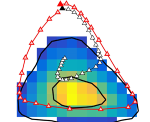
Figure 5 shows how the PFO can be used to extract the probability distributions of the causes and effects of a given observation. Figure 5(a) assumes that we know that the system is within the cell marked with a solid circle at $t=0$. The conditional probability distribution at $t=T$ is given by the corresponding column of the transfer operator, $\boldsymbol{\mathsf{{P}}}^e$, and is displayed in the figure in dashed blue contours. Conversely, the conditional probability distribution of causes at $t=-T$ is the corresponding column of the backwards operator $\boldsymbol{\mathsf{{P}}}^c$. It is displayed in solid black lines, and the difference between the two distributions illustrates the temporal evolution of the system in the clockwise direction of the figure, as in Jiménez (Reference Jiménez2015).

Figure 5. (a) For the variables in figure 4(a), and an interval $T^*=0.076$, the solid black contours are the probability distribution of possible $T$-precursors to an observation of the cell marked with a solid circle, and the dashed blue contours are the distribution of possible effects after $T$. Contours contain 30 % and 95 % of the probability mass. (b) As in (a), for an observation in the core of the invariant density distribution. (c) Mean system displacement in the parameter plane. The coloured background is the invariant density, and the arrows join the cell taken as cause with the mean system location after time $T$. (d) As in (c), but the arrows join the mean location of the systems that will pass through the cell taken as reference, after time $T$. The red contours contain 30 % and 95 % of the invariant density. (e,f) As in (c,d), but using randomised time stamps for the data.

The segregation into forward and backward distributions does not hold for all cells. Figure 5(b) applies the procedure to a cell in the high-probability core of the invariant density distribution. Its forward and backward distributions are marked as in figure 5(a), but they overlap each other and are difficult to tell apart.

Figure 5(c) is a representation of this mean displacement for all the cells in the distribution. The arrows join the centre of each reference cell to the mean position of its effects after a given time interval. Figure 5(d) does the same for the causes, and both figures show a mean clockwise displacement of the system along the upper edge of the distribution (see figure 3(b) in Jiménez Reference Jiménez2015, for comparison). In addition to this circular displacement, the arrows spiral towards the centre of the distribution in figure 5(c), and outwards in figure 5(d). This tendency increases for longer time intervals, and is due to the non-Markovian component of the probability evolution.

Any random displacement from the periphery tends to move towards the most probable locations in the central part of the distribution, and random displacements ending in the periphery are most likely to come from the core. This is best seen in figure 5(e,f), which is computed in the same way as figure 5(c,d) after randomly shuffling the time stamps of the flow snapshots. In fact, since temporal relations are destroyed by the shuffling, effects and causes become randomly chosen states of the system and their conditional average coincides with the overall mean of the invariant distribution. These randomised figures are independent of the time interval.

3.2. Quality indicators

We have mentioned several times that the main problem in constructing the PFO is collecting enough data to populate the two-dimensional histogram, $\boldsymbol{\mathsf{{Q}}}$, making it unpractical to consider distributions over more than two independent variables. We have also mentioned that our strategy is to test many possible variable pairs in the hope of identifying couples whose statistical behaviour is optimal, but the 36 variables used in figure 3 can be paired into 630 possible ways, and automating the search requires indicators that are simpler to implement than the visual inspection of the two-dimensional plots in figure 5. Four such indicators are discussed in this section.

The statistical uncertainty of the displacement vectors is addressed in figure 6(a), which displays the ratio between the standard deviation of the conditionally averaged displacement of the system over a given time and its mean. To compensate for the different magnitudes of the two variables in the figure, which generally have incompatible units, each of them is normalised with its global standard deviation before computing the conditional statistics. The result is a measure of the error bars associated with each of the arrows in figure 5(c).

Figure 6. As in figure 4. (a) Ratio between the averaged displacement of the effects and their standard deviation. The aspect ratio of the geometry normalises each variable with its overall standard deviation to compensate for the different units. (b) Determinacy index (3.5) between the average displacement of causes and effects. Drawn for $T^*=0.025$. (c) Hellinger segregation index (3.6) between the forward and backwards conditional distributions, as function of the observation cell. (d) Kullback–Leibler information gain (3.8) from the distributions of the effects and the causes, measured in bits. Warm colours represent creation of information, and cooler ones represent information loss. All panels refer to the [10] mode of the wall-normal velocity, and use only cells within the 95 % probability contour of $\boldsymbol {q}_\infty$. In all panels, except (b), $T^*=0.076$.

Having a small relative standard deviation does not guarantee that a quantity is physically relevant. Inspection of figure 5(c–f) reveals that deterministic and random evolutions behave differently with respect to the asymmetry between causes and effects. The displacement vectors of the causes and effects rotate in the same direction in figure 5(c,d), because both represent the deterministic evolution of the system. But the randomised vectors in figure 5(e,f) point in opposite directions, because they move from the conditioning cell towards the densest part of the distribution, independently of the direction of time. As a consequence, we can define a ‘determinacy’ index for an observation cell $\boldsymbol {v}_0$ as the normalised inner product

(3.5)\begin{equation} C_{ce}(\boldsymbol{v}_0, T)= \frac{ (\boldsymbol{v}^e-\boldsymbol{v}_0)\boldsymbol{\cdot} (\boldsymbol{v}_0-\boldsymbol{v}^c)} {\|\boldsymbol{v}^e-\boldsymbol{v}_0\| \|\boldsymbol{v}_0-\boldsymbol{v}^c\|}, \end{equation}

where $\boldsymbol {v}^e-\boldsymbol {v}_0$ and $\boldsymbol {v}_0-\boldsymbol {v}^c$ are, respectively, the conditionally averaged displacement of effects and causes over the time interval $\pm T$. As in figure 6(a), variables are normalised with their standard deviation before computing (3.5). This index is an indication of how deterministic is the evolution of the system in the neighbourhood of $\boldsymbol {v}_0$, and of how much information is gained by the observation of the variable pair. When the system is completely deterministic in the subspace being considered, $C_{ce}\approx 1$, and when it is essentially random, $C_{ce}\approx -1$. Figure 6(b) displays $C_{ce}$ for the data in figure 5, and shows that the evolution of this particular Fourier mode is deterministic almost everywhere in this parameter plane.

Along the upper edge of the distribution, this agrees with the physically based conclusions of Jiménez (Reference Jiménez2015), but not along its lower edge, where both Jiménez (Reference Jiménez2015) and Encinar & Jiménez (Reference Encinar and Jiménez2020) conclude that the average displacement is opposite to the predictions of the model that explains the upper edge, and that the uncertainty of the displacements is too large for the means to be trusted. The high uncertainty in this region is clear in figure 6(a), but figure 6(b) suggests that this part of the distribution is also deterministic. Part of the reason is the longer time interval used in figure 6(a) compared with 6(b). The apparent randomness of the evolution increases for longer intervals, as the non-Markovian behaviour takes over. The determinacy index is almost unity in figure 6(b), where the displacements are of the order of one distribution cell, but decreases to $C_{ce}\approx 0.8$ when the figure is drawn for the more physically relevant time interval used in figure 6(a), and decreases further to $C_{ce}\approx 0.5$ for the even longer interval used in Jiménez (Reference Jiménez2015). Encinar & Jiménez (Reference Encinar and Jiménez2020), who use a different method from the one above, and a different set of data, compute a figure of merit equivalent to the relative dispersion in figure 6(a). Normalising their time offset with the average distance, $\bar {y}$, from the wall of their filtered fields (Flores & Jiménez Reference Flores and Jiménez2010; Jiménez Reference Jiménez2015), it varies between $u_{\tau } T/\bar {y} = 0.048$ and 0.19. The resulting standard deviations are negligible for the shortest of those intervals, but large enough to reverse some of the displacements for the largest one. When these values are applied to the present case, assuming $\bar {y}\approx 0.3$ for our integration band, the time interval in figure 6(b) is $u_{\tau } T/\bar {y} = 0.087$, and that in figure 6(a) is $u_{\tau } T/\bar {y} = 0.26$, explaining the apparent discrepancy between figures 6(a) and 6(b).

Figure 6(c) quantifies the temporal segregation between the conditional probability distributions of causes and effects in figure 5(a,b). The distance between two normalised probability distributions $\boldsymbol {q}^{(1)}$ and $\boldsymbol {q}^{(2)}$ can be characterised by the Hellinger norm (Nikulin Reference Nikulin2001), defined as

(3.6)\begin{equation} H^2(\boldsymbol{q}^{(1)},\boldsymbol{q}^{(2)}) = \frac{1}{2} \sum_j \left(\sqrt{q^{(1)}_j}-\sqrt{q^{(2)}_j}\right)^2 , \end{equation}

which vanishes for $\boldsymbol {q}^{(1)}=\boldsymbol {q}^{(2)}$, and reaches its maximum, $H=1$, for disjoint distributions. In the case of figures 5(a,b) and 6(c), the distance between the conditional distributions of causes and effects varies from $H\approx 0.9$ at the edge of the density distribution, where they are clearly different, to $H\approx 0.1$ at the centre, where past and future are almost indistinguishable.

The information provided by the indices (3.5) and (3.6) is related but not identical. While a high value of (3.6) implies that causes and effects are different, a high value of (3.5) also shows that the directions of the mean drift associated with each of them are similar, and that the flow of probability can be described as a smooth vector field.

When figure 6(a–c) is considered, together the panels suggest that the top-right and top-left edges of the probability distribution are populated by systems which evolve in a fairly deterministic manner, while the lower edge of the distribution, and especially its central core, are more random.

Finally, figure 6(d) addresses the question of whether this evolution has any effect in the probability distribution of the variables used in this section; in essence, whether the effects conditioned to a given cell are more or less organised than its causes. The Kullback–Leibler information of a distribution $\boldsymbol {q}^{(1)}$, relative to a reference distribution $\boldsymbol {q}^{(2)}$, is defined as

(3.7)\begin{equation} K(\boldsymbol{q}^{(1)},\boldsymbol{q}^{(2)}) = \sum_j q^{(1)}_j \log_2 (q^{(1)}_j/ q^{(2)}_j), \end{equation}

which is measured in bits, is always non-negative and only vanishes when $\boldsymbol {q}^{(1)}=\boldsymbol {q}^{(2)}$. Intuitively, it describes how much more organised is $\boldsymbol {q}^{(1)}$ compared with $\boldsymbol {q}^{(2)}$. Note that (3.7) is only finite if the support of $\boldsymbol {q}^{(1)}$ is within the support of $\boldsymbol {q}^{(2)}$, so that $K$ can be understood as a measure of how much information is gained by restricting $\boldsymbol {q}^{(2)}$ to one of its subsets. Here, we will always use as reference the invariant distribution $\boldsymbol {q}_\infty$, so that $K$ is guaranteed to exist both for the distribution $\boldsymbol {q}^c$ of the conditional causes and for the distribution $\boldsymbol {q}^e$ of the effects. This choice also implies that a distribution with $K=0$ is statistically indistinguishable from $\boldsymbol {q}_\infty$, and represents an unconstrained set of phase points. The assumption that the system is restricted to a single cell at $t=0$ almost guarantees that information is lost when this concentrated distribution is allowed to spread in the past or in the future, but the information contained in the two distributions cannot be compared directly, because they do not generically share a common support. Figure 6(d) displays the difference

(3.8)\begin{equation} K^{ce} = K(\boldsymbol{q}^e,\boldsymbol{q}_\infty)-K(\boldsymbol{q}^c,\boldsymbol{q}_\infty), \end{equation}

between the information of conditional effects and of conditional causes with respect to the reference. It is positive along the left (growth) edge of the distribution, and negative along the right (decay) edge, suggesting that coherence is first created and later destroyed as the system drifts clockwise. Because the system is stationary, the two effects cancel, and the mean generation of information vanishes.

The real power of the four indicators just described is in the large-scale screening of less obvious variable pairs. Figure 7 displays the value of the determinacy (3.5) and segregation (3.6) indices for all the combinations of modal inclination and intensity of the three velocity components, averaged over the corresponding distributions. Not surprisingly, the most deterministic combinations are those involving the inclination and intensity of the same Fourier mode, but it is interesting that $v_{10}$, which was the mode selected on physical grounds in Jiménez (Reference Jiménez2015), is also the most deterministic by a substantial margin. Slightly less deterministic is $v_{20}$, which is a harmonic of $v_{10}$ for which the same theory applies. The meandering modes, $v_{11},\,v_{21},\,u_{11},\,u_{21}$, are less organised but not fully incoherent. The spanwise velocity is not well described by an inclination and an intensity, but an interesting pair is $(I_{v11}, I_{w11*})$ or $(I_{v11*}, I_{w11})$, which was already identified as an inclined roller from the correlations in figure 3. Its appearance in the two indicators in figure 7 shows that this roller has its own causal dynamics, and that the same is true for the second harmonic, $(I_{v21}, I_{w21*})$. Interestingly, the streamwise-uniform roller $(I_{v01}, I_{w01*})$ does not appear in figure 7, even if it is one of strongest pairings in the correlations in figure 3, and one of the largest contributors to the fluctuation energies in figure 2. Such two-dimensional streamwise structures do not interact with the shear and, even if they grow to be strong, have little own dynamics.

Figure 7. As in figure 3. (a) Determinacy index (3.5), averaged over the invariant distribution for different combinations of modal inclination and intensity. (b) Segregation index (3.6). The main diagonal and the inclinations of the $k_x=0$ modes are blocked in magenta in both cases.

Figure 8 displays the drift diagram and two quality indicators for the $(I_{v11}, I_{w11*})$ roller. The two variables are relatively well correlated, probably by continuity, but the distribution rotates counter-clockwise. This implies that the roller is first created as an ejection (or sweep) of the wall-normal velocity, and later spreads spanwise. Figure 8(c) shows that, as in figure 6(d), coherence is created when the structure strengthens, and destroyed when it weakens.

Figure 8. As in figures 5 and 6, for the roller variables, $(I_{v11}, I_{w11*})$. (a) Quiver plot of the effects, as in figure 5(c), $T^*=0.076$. (b) Determinacy index (3.5), as in figure 6(b), $T^*=0.025$. (c) Kullback–Leibler information gain (3.8), as in figure 6(d), $T^*=0.076$.

3.3. Conditional averages

The analysis in the previous sections reveals which variable pairs evolve in a deterministic way, but says little about the associated flow fields. A first step in that direction is figure 9, which displays the averages of other flow variables conditioned to the basic $(\psi _{v10},I_{v10})$ pair. Most conditional averages provide relatively little information. They are either distributed almost uniformly over the invariant probability distribution, or track the evolution of the base variables, saying little more than that strong structures are strong in most variables. A few are more interesting.

Figure 9. (a–c) Average intensity of different velocity modes, conditioned to the variable pair $(\psi _{v10},I_{v10})$: (a) $u_{10}$, (b) all modes of $u$ with $k_z\ne 0$, (c) $\sqrt {v^2_{11}+w^2_{11}}$. (d–f) Conditioned to $(I_{v11}, I_{w11*})$: (d) $u_{11}$, (e) $u_{10}$, (f) all modes of $u$ with $k_z\ne 0$. (g–i) Conditional tangential Reynolds stress, $\theta$: (g) all the retained harmonics, (h) $\theta _{10}$, (i) all harmonics with $k_z\ne 0$.

Figure 9(a) shows that the streamwise velocity becomes more non-uniform in the streamwise direction $(u_{10})$ as the wall-normal velocity bursts. It follows from the choice of conditioning variables that this is also true for the wall-normal velocity, but is not true for the spanwise component (not shown). The coupling of $u_{10}$ and $v_{10}$ is required by continuity, and the two variables are part of the two-dimensional burst described in Orr (Reference Orr1907) and Jiménez (Reference Jiménez2013). However, self-sustaining turbulence requires three-dimensionality, and this is provided by the $k_z\ne 0$ modes in figure 9(b). This figure displays the sum of all the modes of $u$ that form a possibly non-uniform streak. They grow along the decay leg of the burst, and are therefore probably consequences, rather than precursors of the burst. It can be shown that most of the growth in figure 9(b) is due to the [01] mode, which measures the intensity of a streamwise-uniform streak, and is also responsible for most of the asymmetry of the figure along the $\psi$ axis. The higher modes, [11] and [21], only grow weakly, and do so along the ascending leg of the burst. On the other hand, the cross-flow $(v,w)$ roller grows along the descending branch, as shown in figure 9(c) for the [11] harmonic. This is also true for the [01] streamwise roller, which has similar intensity, but much less for the [21] mode, which is weaker and less coherent. In all these cases, the two signs of $k_z$ are grouped in the figure.

When the intensity of the $x$-dependent modes is substituted by a non-uniformity index

(3.9)\begin{equation} \varOmega_{a,mn} =I_{a,mn}/I_{a,0n}, \end{equation}

figure 9 changes somewhat. The growth of the roller in figure 9(c) is transferred to the bottom of the distribution. Its non-uniformity begins with $w_{11}$ in the descending leg of the burst, and moves to $u_{11}$ and $v_{11}$ along its left-going bottom edge. This wavy quasi-streamwise roller is very weak in that region, but also very non-uniform, and it is tempting to conclude that its waviness is part of what eventually triggers a subsequent burst.

Figure 9(d–f) shows conditional averages in the plane of the $(I_{v11}, I_{w11*})$ meandering roller. Figure 9(d) is equivalent to figure 9(a), and confirms that the roller is a three-dimensional structure in which the streamwise velocity increases as $v_{11}$ and $w_{11*}$ do. The effect is much stronger for $u_{11}$ than for $u_{11*}$, showing that the active streamwise velocity is collocated with the wall-normal component, $v_{11}$, rather than with $w_{11*}$. The three-dimensionality extends to other harmonics, and figure 9(e) shows that one effect is to enhance the streamwise non-uniformity of the spanwise-uniform component $u_{10}$. This figure is dual to figure 9(a), and suggests that the intensification of the roller takes place along the upper edge of the $(\psi _{v10},I_{v10})$ burst, although where exactly cannot be decided from this representation. For example, the conditional $I_{v10}$, which would be a direct indicator of the position along the $(\psi _{v10},I_{v10})$ burst, does not produce a clear signal in the $(I_{v11}, I_{w11*})$ plane. Figure 9(f) shows the conditional $k_z\ne 0$ component of $u$, which is the same quantity in figure 9(b), and gives more information. Figure 9(b) shows that the streak of $u$ grows along the descending leg of the clockwise evolution of $(\psi _{v10},I_{v10})$, while figure 9(f) shows that it grows along the ascending leg of the counter-clockwise evolution of $(I_{v11}, I_{w11*})$. Both legs therefore presumably correspond to the same stage of the flow, in agreement with the location in figure 9(c) of the high roller intensity.

Also interesting is figure 9(g–i), which shows the conditional tangential Reynolds stress, $\theta _{mn}=-{\rm Re} (\tilde {u}_{mn} \tilde {v}^{\dagger} _{mn})$, integrated as in (3.2). Although the quantity in the equations of motion is $\partial _y\theta$, rather than $\theta$ itself, a positive stress tends to make the mean velocity profile more turbulent, steeper near the wall, and negative ones tend to lower the wall shear. Figure 9(g) displays the conditional Reynolds stress due to all the retained harmonics, which we saw in § 3 to account for approximately two thirds of the total flow stress. It is positive everywhere, and stronger in the upper edge of the distribution, where other flow features are also strong. It is also asymmetric in the $(\psi _{v10},I_{v10})$ plane, stronger during the growth of the burst than along its decay. The reason is shown in figure 9(h), which displays the stress due to the Orr (Reference Orr1907) harmonic, $\theta _{10}$. It is almost antisymmetric in $\psi _{v10}$, positive during the growth of the burst and negative during its decay. This is what makes the burst transient, since its decay undoes the effect of the growth. The [10] mode is the only one that generates counter-gradient stresses. Figure 9(i) displays the tangential stresses from all the other modes. They are positive everywhere, and the net effect of the burst, although transient in itself, is to generate a three-dimensional structure along its decay leg.

Although not shown in the figure, it is interesting that, when $\theta _{10}$ is conditioned to the $(I_{v11}, I_{w11*})$ plane, it is also negative in the uppermost tip of the roller distribution, confirming our previous conclusion that strong rollers correspond to the burst decay.

In a loose sense, both the down-going right-hand edge of the probability distribution in figure 9(a–c) and the up-going right-hand edge of figure 9(d–f), portray the evolution of a non-uniform $u$-streak into a $(v,w)$ roller. In the top row of figure 9 we see the decay of the streak, and in the middle one we see the growth of the roller. The comparison of the conditioned variables in both sets of figures suggests that the coherent right-hand edge of the evolution of the roller corresponds to the decay of the burst, so that the approach to the lower-right vertex of the triangle in figure 9(a–c) corresponds to the top of the distribution in figure 9(d–f). In this interpretation, the low-intensity evolution of the burst along the bottom edge of the distribution in figure 9(a–c) should correspond to the decay of the roller along the left edge of the distribution in figure 9(d–f). This phase of the burst will be examined in more detail in the next section.

4. Conditional trajectories

It may be useful at this point to recall that the maps in figures such as 9 are not the PFO, but its leading eigenvector rearranged as a two-dimensional matrix for human convenience. The operator itself is the larger matrix in figure 4(b), or a stack of such matrices at different time intervals. The maps in figure 9 are probability distributions of the state of the flow in phase space, and the delta-function distribution used to generate figure 5(a,b) represents a measurement that particularises that probability to a combination of variables describing a given flow configuration. For the rest of the paper we will study these collapsed probabilities, and the statistical properties of the trajectories connecting two or more such states. The PFO then becomes mostly a guide to which cells can be expected to provide the most interesting information, and to how the trajectories connecting them should be chosen.

For example, consider the statistical characterisation of trajectories that satisfy conditions at two different times, such as in the recurrence test in which approximate periodic behaviour is identified by monitoring when a trajectory approaches itself after a given delay (Kawahara, Uhlmann & van Veen Reference Kawahara, Uhlmann and van Veen2012). The statistical equivalent is whether the conditional probability distribution of the effects of a given cell includes the conditioning cell after some delay. In practice, this reduces to identifying among the diagonal of the matrix $\boldsymbol{\mathsf{{P}}}^e(T)$ those cells that result in maximum probability of recurrence for each time delay. An example is figure 10(a), which plots the maximum of the diagonal of the PFO for the $(\psi _{v10},I_{v10})$ plane. It is unity at $T= 0$, when trajectories are still at their initial position, and quickly decays to approximately 0.05, which is the probability that a random trajectory intersects some cell in the core of the invariant distribution $\boldsymbol {q}_\infty$. However, the curve peaks again at $T^* = 0.66$, and, interestingly, at twice that delay, $T^* = 1.35$. Moreover, since the PFO contains information about all the cells in the distribution, it allows us to recover which conditioning cell is responsible for the probability maximum, and therefore which cell has the highest probability of recurring. This is marked as ‘B’ (for burst) in figure 10(b), and turns out to be an extreme high-amplitude event beyond the 95 % threshold used up to now as the practical edge of our distribution. In the trajectories discussed in this section, closed symbols mark the position at $t=0$, and the open triangles along some trajectories are equispaced by $\Delta t^*=0.025$.

Figure 10. (a) Recurrence test for trajectories in the $(\psi _{v10},I_{v10})$ plane. See text for explanation. (b) Black symbols are the mean trajectory passing through the most probable recurrent cell, for the period marked by the dark circle in (a). The red symbols are the only recurrent orbit crossing that cell, which is thus responsible for the local maximum in (a). (c) As in (b), in the $(I_{v11}, I_{w11*})$ plane of the meandering roller. (d) As in (b) but all the non-recurrent trajectories are plotted as simple lines, each one starting with a solid circle.

Two other cells are labelled in figure 10(b), marking the right- (‘R’) and left-hand (‘L’) corners of the triangular distribution. We will maintain this nomenclature for the rest of the section, with some adjustments in the location of the cells. Trajectories spanning the up-going (${\rm L} \to {\rm B}$), down-going (${\rm B} \to {\rm R}$) and bottom (${\rm R} \to {\rm L}$) legs of the periphery of the triangle will be denoted as growth, decay and recovery trajectories, respectively. The growth and decay legs form the burst (Jiménez Reference Jiménez2013). The upper half of these two legs is deterministic, and can be predicted linearly (Jiménez Reference Jiménez2015), but linearised bursts do not recur. There is no obvious theory for the bottom recovery leg, which is required if bursting is to explain self-sustaining turbulence. Most of this section is dedicated to analysing the recovery process.

Out of our $5\times 10^4$ snapshots, only eight trajectories cross the extreme B in figure 10. Most of them do not recur, and the line of open black triangles in figure 10(b) traces the average conditional trajectory during the recurrence period. As is true for most trajectories, it approaches the high-probability core of the distribution. However, individual trajectories can be tested, and the line of red triangles in figure 10(b) shows the trajectory responsible for the peak in figure 10(a). Centring ourselves on this orbit, its growth, decay and recovery legs last approximately $T^*=0.25$, $0.25$ and 0.16, respectively, for a total recurrence time $T^* \approx 0.66$, as in figure 10(a). The total length of its two bursting legs, $T^* \approx 0.5$, also agrees with the width of the bursting correlations for this flow in Jiménez (Reference Jiménez2015).

Although the recurrent trajectory very approximately closes on itself in the plane of figure 10(b), its recurrence is weaker when more variables are included. For example, figure 10(c) plots the same trajectories in the plane of the $(I_{v11}, I_{w11*})$ roller. As before, the recurring trajectory is displayed as red triangles. It loiters for a while near the high-probability core of the $(I_{v11}, I_{w11*})$ distribution, and joins the counter-clockwise coherent circulation during the growth period of the $(\psi _{v10},I_{v10})$ burst. The black triangles of the mean trajectory are again very different from the recurrent one, and never join the coherent circulation.

However, the divergence between the recurrent trajectory and the other trajectories that cross B is mostly a long-time phenomenon. This can be seen in figure 10(d), which is equivalent to figure 10(b) but plots all the individual trajectories going through B. The recurrent orbit is still plotted with open red triangles, while other trajectories are plotted as lines of different colours without symbols, in no particular order. All the trajectories in the figure start from the same cell and behave similarly for a while. It is only after they have decayed to approximately half their initial $I_{v10}$ that they deviate towards the high-probability core. A similar plot in the $(I_{v11}, I_{w11*})$ plane, not shown, shows the same trends, although slightly more complicated because trajectories do not start in the same cell any more. The recurrent orbit is special in that it starts with a relatively weak and decaying roller, which only strengthens towards the end of the orbit. This is probably the reason why its $(\psi _{v10},I_{v10})$ projection is able to proceed undisturbed for a relatively long time.

That the approximately recurrent orbit includes an infrequent extreme event suggests that it may not be very relevant to the flow statistics, or even to its evolution. Its interest resides in that it includes a recovery leg that traverses the lower edge of the parameter space in the ‘wrong’ direction, showing that coherent recovery connections exist, and suggesting how to study them. The question is whether other trajectories exist that cross the lower edge of the distribution in the same direction, even if they do not follow the recurrent orbit around the full $(\psi _{v10},I_{v10})$ plane.

Figures 11 and 12 address this question. Figure 11(a,b) is equivalent to the cause and effect distributions in figure 5(a), but applied to the R and L corner cells for several values of the delay interval. Even if we saw in figure 6(a) that the lower edge of the distribution is a region of large scatter for the system drift, figure 11(a) shows that the flow propagates steadily from R towards L as the delay increases, and that it only spills slowly into the high-probability core of the distribution. The same is true for the causes of cell L in figure 11(b). When similar plots are drawn for a cell in the central part of the lower edge of the distribution, the drift is slower and the scatter higher (not shown), suggesting that the propagation in figure 11(a,b) can be interpreted as a direct connection between R and L that bypasses some of the intermediate states of the probability distribution.

Figure 11. Probability distributions of the causes and effects for several delay intervals, as in figure 5(a,b). (a) Effects conditioned to the cell marked as R in the lower right-hand corner of the invariant density distribution. From blue to yellow, $T^* = 0.025 (0.025) 0.15$. (b) As in (a), for the causes leading to the cell marked as L in the lower left-hand corner.

Figure 12. (a–c) Grey lines are the phase trajectories that cross a causal cell at $t=0$. Blue ones are those that also cross the effect cell within a given range of time intervals. (a) Growth leg of the burst, from ${\rm L} \to {\rm B}$ in $T^* = 0.2\unicode{x2013}0.3$. (b) Decay from ${\rm B} \to {\rm R}$ in $T^* = 0.2\unicode{x2013}0.3$. (c) Recovery leg from ${\rm R} \to {\rm L}$ in $T^* = 0.15\unicode{x2013}0.175$. (d–f) Averaged evolution of the flow along the blue trajectories in (a–c), respectively, reconstructed from the retained harmonics. Flow is from bottom left to top right, and time increases from top to bottom. Translucent orange isosurface, $u^+=0.7$; translucent grey, $u^+=-0.7$; cyan, $v^+=0.4$; purple, $v^+=-0.4$. Panels (d–e) show $t^*=0.075 (0.05) 0.225$. Panel (f) shows $t^*=0 (0.05) 0.15$, and $v^+=\pm 0.3$.

This is further analysed in figure 12(a–c). Each of these panels represents a leg of the burst that traverse the periphery of the distribution in the $(\psi _{v10},I_{v10})$ plane. For example, figure 12(a) represents the growing leg, from the cell marked as L to the one marked as B (note that the latter has been chosen substantially lower than in figure 10, to bring it within the 95 % probability contour). It takes the system $T^* \approx 0.25$ to move from one to the other, and the grey lines are the $O(500)$ trajectories that pass through L at $t=0$. Of these, only the six trajectories drawn in blue also pass through B in the interval $T^* = 0.2\unicode{x2013}0.3$. Figure 12(b,c) is similarly drawn for the decay and recovery legs of the burst, respectively. The trajectories in these three legs are not continuations of each other. For example, there is a single trajectory linking cells L, B and R, in that order, three trajectories linking R, L and B and no trajectory linking B, R and L. The only trajectory approximating a full cycle in this plane is the one in figure 10.

This lack of continuity is a direct consequence of the non-Markovian behaviour discussed in § 2 and in figure 4(c). Cell R is not the initial condition for cell L, or for the recovery leg, but only the projection onto the $(\psi _{v10},I_{v10})$ plane of many initial conditions, most of which will not fully follow that leg or continue into the growth one. In moving from probabilities based on one cell to two-point trajectories, we have in essence abandoned the two-dimensional PFO for a higher-dimensional version based on the state of the system at two points in time. In a different interpretation, we have moved from a Markovian probabilistic predictor to a more complex dynamics.

Figure 12(d–f) displays the mean evolution of the flow field, reconstructed from the retained harmonics along the blue trajectories in figure 12(a–c), respectively, with time increasing from top to bottom. Because the problem is homogeneous in $x$ and $z$, the flow in the different trajectories has to be aligned to a common origin before averaging. This is done at $t=0$ by translating each case so that the deepest low-speed perturbation of the streamwise velocity is located at the centre of the display box. To facilitate visual tracking, the frame of reference is then advected with a velocity $U_{ad}^+=8$, which keeps the structures approximately stationary near the wall.

The forward tilting of the $v$-structures by the shear is clear in the growth and decay legs of the burst (figure 12d,e). The recovery leg in figure 12(f) is harder to interpret, in part because everything is much weaker than in the other two cases, but the clearest difference is that, while the growth and decay are dominated by high-streamwise-velocity structures near the wall, the high-speed regions of the recovery leg are predominantly farther into the flow. The near-wall layer only contains a weak discontinuous low-speed streak. Since the structures in figure 12(d–f) are defined with respect to a long-term-averaged velocity profile, this difference in organisation implies that the box-averaged instantaneous velocity profile differs among legs.

This is confirmed in figure 13(a,b), which shows that the burst is characterised by high velocities and steep profiles near the wall. Figure 13(c) shows that the recovery takes place in regions where the velocity is lower near the wall, and the shear is displaced away from it. The flow enters the recovery leg with a steep velocity gradient at $y/h\approx 0.2$, which decays as the recovery proceeds (red to blue). Figure 13(d–f) shows the evolution of the fluctuation energy at the same times. During the burst, in figure 13(d,e), the fluctuations stay relatively close to the wall $(y/h\approx 0.12)$, and the energy peak extends all the way to it. During the recovery leg, in figure 13(f), a new peak grows at the location of the detached shear layer $(y/h\approx 0.22)$, and forms a new secondary peak at the wall.

Figure 13. Box-averaged velocity profiles, for the trajectories marked in blue in figure 12. (a–c) Mean velocity, $\tilde {u}_{00}$. (d–f) Kinetic energy of the retained harmonics. (a,d) Growth leg. (b,e) Decay leg. (c,f) Recovery. Time increases from red to blue, separated by $t^*=0.025$ among curves.

Note that the streamwise velocity perturbations in most panels of figure 12(d–f) are short and discontinuous, in agreement with the recent evidence in Jiménez (Reference Jiménez2022) that long streaks are not directly linked to the regeneration cycle of wall turbulence.

The conclusion that the recovery of the burst depends on a low-shear region near the wall is inconsistent with the intuitive notion that, since the shear is the ultimate source of turbulent energy, a higher shear should be a prerequisite for higher turbulent activity. Indeed, it has been known for some time that turbulent intensity and shear are correlated (Marusic, Mathis & Hutchins Reference Marusic, Mathis and Hutchins2010; Jiménez Reference Jiménez2012; Mathis et al. Reference Mathis, Marusic, Chernyshenko and Hutchins2013), but the implied model is usually that the turbulence intensity evolves to be in equilibrium with the shear. Our discussion suggests that the causality is the other way around (figure 9), and that the shear is created by the Reynolds stresses of the fluctuations. In fact, since the mass flux in our channels is constant, a low shear near the wall implies a higher one further up. What our previous discussion suggests is that the decay of a burst induces a mild shear at the wall, which in turn steepens the velocity profile away from it. The steep off-wall profile is what triggers the new burst, which is the blue/magenta structure growing away from the wall in the downstream part of figure 12(f). Flores & Jiménez (Reference Flores and Jiménez2010) showed that stress waves travel to and from the wall in small-box simulations such as the present one, with a wall-normal velocity of the order of $u_{\tau }$. It is difficult to decide from such kinematic observations which of the two directions is the primary causal one, but the discussion above suggests that at least the descending wave is causal, in agreement with previous reports that the structure of the logarithmic layer in wall-bounded flows is relatively independent from the details of the wall, which is therefore not the primary, or at least not the only, seat of causality (Townsend Reference Townsend1976; Mizuno & Jiménez Reference Mizuno and Jiménez2013; Kwon & Jiménez Reference Kwon and Jiménez2021).

5. An interventional experiment

The analysis in the previous sections gives strong hints about which variables evolve coherently in wall-bounded flows, and about how this evolution can be interpreted in terms of causality within the attractor in phase space. However, the second question posed in the introduction, whether this information has any practical value, generally takes us outside the attractor, and can only be answered by more classical interventional experiments or by theoretical models. Strictly speaking, this is beyond the scope of the present paper, whose goal is to develop a methodology and to give examples of how it can be used to motivate more classical work, but we present in this section an example of how that work might proceed, building on our discussion of figure 12.

The main result of that discussion is that a particular, weakly sheared, configuration of the mean velocity profile is a requirement for burst recovery. This is not a new idea: what is probably the oldest theory of how wall turbulence is controlled is based on the two-way interaction between shear and turbulence intensity (Malkus Reference Malkus1956). It is also known that forcing a locally steeper or shallower velocity profile leads to equilibrium intensities that correlate with the local shear (Tuerke & Jiménez Reference Tuerke and Jiménez2013), and many low-order models of the turbulence cycle include a variable that stands for the mean velocity profile (Waleffe Reference Waleffe1997).

However, the original linear version of the Malkus (Reference Malkus1956) model was disproved by Reynolds & Tiederman (Reference Reynolds and Tiederman1967), who found no trace of the marginal instability of the velocity profile that that model assumes for turbulent channels, and the analysis in Waleffe (Reference Waleffe1997), although highly suggestive because the effect of a strong wall shear is to inhibit the instability of the streaks, only applies to permanent travelling waves in marginally turbulent low Reynolds number flows. Similarly, Tuerke & Jiménez (Reference Tuerke and Jiménez2013) refer to long-term flow averages, and it is unclear whether these are relevant to the short-term behaviour of an intermittent bursting cycle. The hypothesis to be tested is whether a feedback cycle involving the modification of the mean profile by the turbulent fluctuations, and the control of the latter by the former, can explain at least part of the mechanism that sets the frequency and amplitude of the bursts.

We do this by smoothing the evolution equation that links the fluctuations to the mean profile, defined as the deviation from the long-term mean velocity profile of the $(x,z)$-averaged streamwise velocity fluctuation, $\tilde {u}_{00}(y)$. In a regular channel it satisfies

(5.1)\begin{equation} \partial_t\tilde{u}_{00} = R-{P} + \nu\partial_{yy} \tilde{u}_{00}, \end{equation}

where $R=-\partial _y(\widetilde {uv})_{00}$ is the instantaneous mean Reynolds-stress gradient, and the pressure gradient $P$ is determined by the ancillary flux-conservation condition

(5.2)\begin{equation} \int_0^{2h} \tilde{u}_{00} \,{\rm{d}} y= 0. \end{equation}

In our experiment, we substitute (5.1) by

(5.3)\begin{equation} \partial_t\tilde{u}_{00} = Q-{P} + \nu\partial_{yy} \tilde{u}_{00}, \end{equation}

where

(5.4)\begin{equation} \partial_tQ = (R-Q)/\tau, \end{equation}

which, after a transient in which the effect of the initial conditions decays exponentially, is solved by

(5.5)\begin{equation} Q(y,t) = \tau^{-1} \int_0^t \exp[(\xi-t)/\tau] \, R(y,\xi) \,{\rm{d}}\xi. \end{equation}

The modified right-hand side, $Q$, is therefore a smoothed version of $R$, with a smoothing time $\tau$. The integral of $R$ or $Q$ across the channel can be considered as a body force that must be compensated by the pressure gradient, but it is easy to see from its expression that $\int R\,{\rm {d}} y =0$ for impermeable walls, and that the same holds for $Q$ after the initial transient.

Figure 14 shows some results from the experiment, using a smoothing time, $\tau ^*=2.27$, of the order of the expected bursting period (Flores & Jiménez Reference Flores and Jiménez2010). Figure 14(a) shows the history of the friction Reynolds number for the natural and modified channels. It only increases slightly for the smoothed case, from $\langle h\rangle ^+=950$ to 975, although its temporal oscillations become much slower. More interesting is figure 14(b), which shows the oscillations of the box-averaged kinetic energy. They are somewhat deeper for the smoothed case, and substantially less frequent and more regular. An approximate count, using a method explained below, gives $\Delta t^*\approx 3.9$ for the mean distance between bursts in the natural case, and $\Delta t^*\approx 5.2$ in the smoothed one. Both are longer than in Flores & Jiménez (Reference Flores and Jiménez2010), who find $\Delta t^*\approx 2$ from the temporal spectrum of the integrated Reynolds stress, probably because their method is sensitive to weaker oscillations than the present one.

Figure 14. (a) Instantaneous friction velocity of the temporally smoothed and natural experiments, (5.1)–(5.4). (b) As in (a), for the box-averaged fluctuating kinetic energy, $E=u'^2+v'^2+w'^2$, measured with respect to its long-time average. (c) Mean velocity profiles. (d) Mean kinetic energy. In all cases: blue, natural channel; red, $\tau ^*=2.27$. (e–h) Temporal evolution of the mean profiles as functions of time. (e,f) Mean streamwise velocity fluctuation, with respect to its long-time average. (g,h) Kinetic energy. (e,g) Natural channel. (f,h) Case $\tau ^*=2.27$.

The effect on the integrated velocity profiles is slight. Figure 14(c) shows the mean velocity, and reveals that the main effect is to decrease the wake component above $y/h\approx 0.3$, but this is also the height at which this channel begins to be constrained by the numerical box, and where the profile in any case deviates from the natural one. Figure 14(d) shows that the fluctuations of the kinetic energy are also slightly higher, as expected from figure 14(b).

Figure 14(e–h) shows the temporal evolution of the profiles, and give more information. Figure 14(e,f) shows the deviation, $\tilde {u}_{00}$, of the mean velocity profile with respect to its long-time average. Each vertical section of these images is an instantaneous box-averaged profile. Blue regions are slower that usual, and yellow ones are faster. They should be compared with the instantaneous profiles in figure 13(a–c), although the flows in figure 14 are not filtered or conditioned in any way. Figure 14(e,g) is the natural flow, and figure 14(f,h) is temporally smoothed. The white dashed vertical lines in figure 14(e–h) mark the time of the bursts of the kinetic energy, whose evolution is represented in figure 14(g,h). To detect them, the kinetic energy is integrated in $y/h\in (0,0.4)$, and bursts are defined as intervals where the integrated energy rises above the level isolating the top 15 % of the time.

The most interesting differences are those between the mean velocities in figures 14(e) and 14(f). The evolution in the natural case in figure 14(e) is clearly more complex than the temporally smoothed case in figure 14(f), and there is no clear correlation between the mean velocity and the position of the bursts marked by the dashed white lines. The opposite is true for the smoothed case in figure 14(f), in which the mean profile rises and falls in a series of diagonal waves, and the lines marking the bursts correspond, even to the naked eye, to low-velocity intervals marked by bluish areas near the wall. The inclined red line in the four panels of the figure mark the friction velocity, ${\rm {d}} y/{\rm {d}} t=u_\tau$, which is known to be the vertical advection velocity of strong Reynolds-stress structures (Flores & Jiménez Reference Flores and Jiménez2010; Lozano-Durán & Jiménez Reference Lozano-Durán and Jiménez2014). This agrees with the inclination of the rising and falling patterns in the energy evolution maps in figure 14(g,h). It also approximately describes the vertical advection velocity of the fine structure of the velocity profiles in figure 14(e), most probably because the mean profile is controlled by the Reynolds stress through (5.1). On the other hand, this influence is broken in figure 14(f), where the Reynolds stresses only acts indirectly on the mean profile because of the smoothing effect of (5.4), and the vertical advection is much slower. This strongly suggests that any correlation between figures 14(f) and 14(h) reflects a causal effect of the mean velocity on the burst, rather than the other way around.

This is directly tested in figure 15, which shows the conditionally averaged temporal evolution of different quantities obtained by centring them on the time of all the detected energy bursts. Figure 15(a) shows the conditional evolution of the mean profile, and clearly shows the low-velocity period preceding the burst, which is later substituted by a steeper wall profile created by the Reynolds stress of the burst, shown in figure 15(b). The conditional Reynolds stress is displayed in figure 15(c), which shows that it is a local effect due to the burst itself. An attempt to repeat this process for the natural flow in figure 15(e,g) fails, no doubt in part because the more complex structure of the flow field makes the identification of the bursts harder. In fact, even the conditioning of the burst on the burst position, as in figure 15(b), fails in that case. The experiment was repeated for smoothing times of the order of two or four bursting periods, with comparable results.

Figure 15. Time evolution of the $(x,z)$-averaged profiles conditioned to the bursts of the kinetic energy in the smoothed experiment. (a) Mean streamwise velocity fluctuation, as in figure 14(f). (b) Kinetic energy. This is the conditioning field. (c) Tangential Reynolds stress, $-(\widetilde {uv})_{00}^+$.