1. Introduction

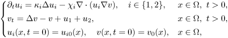
Chemotaxis is a common phenomenon in mathematical biology. Since Keller and Segel [Reference Keller and Segel14] suggested a mathematical chemotaxis model for chemotactic aggregation of the cellular slime mold Dictyostelium discoideum in the early 1970s, a large number of theoretical (mathematical) models, including the chemotactic movement of multi populations along with multiple stimuli in the environment, have been proposed by many researchers (see [Reference Horstmann12]). In this paper, a chemotaxis system for two populations interaction via the same chemical signal will be considered as follows:

(1.1)\begin{equation} \left\{\begin{array}{@{}ll} \partial_tu_1=\kappa_1\Delta u_1-\chi_1\nabla\cdot(u_1\nabla v), & x\in\Omega,\ t>0,\\ \partial_tu_2=\kappa_2\Delta u_2-\chi_2\nabla\cdot(u_2\nabla v), & x\in\Omega,\ t>0,\\ v_t=\Delta v-v+u_1+u_2, & x\in\Omega,\ t>0,\\ u_i(x,t=0)=u_{i0}(x),\quad v(x,t=0)=v_0(x),\ i=1,2, & x\in\Omega, \end{array} \right. \end{equation}

where $u_i$ denotes the population density for the $i$-th population, and $v$ represents the chemical signal concentration. $\kappa _i>0$ is the diffusion coefficient for the $i$-th population and the chemotactic coefficient $\chi _i>0$ measures the strength of the chemical signal with respect to $u_i$. Here the domain $\Omega$ is

(1.2)\begin{equation} \text{either the whole space}\ \mathbb{R}^2\ \text{or a disk}\ \Omega=B_R(0)\subset \mathbb{R}^2\ \text{with some}\ R>0. \end{equation}

When $\Omega$ is the above bounded domain, the system (1.1) is supplemented with homogenous Neumann boundary condition

(1.3)\begin{equation} \partial u_i/\partial\nu=\partial v/\partial\nu=0,\quad i=1,2. \end{equation}

For a two-dimensional domain, one of the most interesting and important question for the chemotaxis system in both biological and mathematical contexts is to determine critical mass phenomenon, namely, the behaviour of the solutions is only dependent on the initial mass of the system. This mass threshold phenomenon was exactly confirmed in the well-known Keller–Segel chemotaxis model for one population:

(1.4)\begin{equation} \left\{ \begin{array}{@{}ll} \partial_tu_1=\kappa_1\Delta u_1-\chi_1\nabla\cdot(u_1\nabla v), & x\in\Omega,\ t>0,\\ v_t=\Delta v-v+u_1, & x\in\Omega,\ t>0,\\ u_1(x,t=0)=u_{10}(x),\quad v(x,t=0)=v_0(x), & x\in\Omega. \end{array} \right. \end{equation}

Let $m_1(u_{10};D)=\|u_{10}\|_1=\int _{D}u_{10}(x)\,{\rm d}x$ for $D\subset \mathbb {R}^2$. Consider (1.4) with boundary condition (1.3) in a bounded domain $\Omega \subset \mathbb {R}^2$. An application of the Moser–Trudinger inequality to (1.4) ensures that the solution exists globally in time provided $m_1(u_{10};\Omega )<4\pi \kappa _1/\chi _1$ for arbitrary smooth domain or $m_1(u_{10};\Omega )<8\pi \kappa _1/\chi _1$ for radial domain [Reference Nagai, Senba and Yoshida21]. Conversely, if $m_1(u_{10};\Omega )>8\pi \kappa _1/\chi _1$, then there exists a blow-up solution in finite time [Reference Herrero and Velázquez10]. Similar to [Reference Herrero and Velázquez10], there also exists a blow-up solution for (1.4) for $\Omega =\mathbb {R}^2$ when $m_1(u_{10};\mathbb {R}^2)>8\pi \kappa _1/\chi _1$. However, it was shown in [Reference Calvez and Corrias3] that the solution with $m_1(u_{10};\mathbb {R}^2)<8\pi \kappa _1/\chi _1$ exists globally over time under the following conditions $u_{10}\log (1 + |x|^2)\in L^1(\mathbb {R}^2)$ and $u_{10}\log u_{10}\in L^1(\mathbb {R}^2)$. While these additional initial data conditions have been completely removed in [Reference Mizoguchi15] by terms of the Moser–Trudinger inequality. Moreover, the critical case $m_1(u_{10};\mathbb {R}^2)=8\pi \kappa _1/\chi _1$ was also studied in [Reference Mizoguchi15], the solutions exist globally or the blow-up set of solutions equals $\mathbb {R}^2$. Because chemicals diffuse much faster than population then it is feasible to study a simple parabolic-elliptic version of (1.4), i.e., the second parabolic equation is replaced with an elliptic form

\[ 0=\Delta v-v+u_1, \quad\text{or}\quad 0=\Delta v+u_1,\quad \text{if}\ \Omega=\mathbb{R}^2, \]

or

\[ 0=\Delta v-v+u_1, \quad\text{or}\quad 0=\Delta v-\mu+u_1,\quad \text{if}\ \Omega\subset\mathbb{R}^2\ \text{is a bounded domain}, \]

where $\mu :=\|u_{10}\|_1/|\Omega |$. We refer the readers to the papers [Reference Biler2, Reference Horstmann11, Reference Jäger and Luckhaus13, Reference Nagai17–Reference Nagai19] for a similar and satisfactory analytical description about the critical mass for these situations in two dimensions. The above results show that $8\pi \kappa _1/\chi _1$ is the critical mass for (1.4), and determines that the solutions exist globally or blow up if $\Omega$ satisfies (1.2).

For multi-population chemotaxis system, a natural question arises: do there exist critical numbers such that whenever the initial masses for populations are smaller than them then the solution will exist globally, whereas the masses are larger then the solution will blow up? Espejo et al. [Reference Conca, Espejo and Vilches5, Reference Espejo, Stevens and Velzquez7–Reference Espejo, Vilches and Conca9] consider a simplified parabolic-elliptic version of two-population system likes

(1.5)\begin{equation} \left\{ \begin{array}{@{}ll} \partial_tu_1=\kappa_1\Delta u_1-\chi_1\nabla\cdot(u_1\nabla v), & \\ \partial_tu_2=\kappa_2\Delta u_2-\chi_2\nabla\cdot(u_2\nabla v), & \\ 0=\Delta v+u_1+u_2, & \text{if}\ x\in\Omega=\mathbb{R}^2,\quad \text{or}\\ 0=\Delta v-\mu'+u_1+u_2, & \text{if}\ x\in\Omega\subset\mathbb{R}^2\ \text{is a disk}, \end{array}\right. \end{equation}

where $\mu ':=(\|u_{10}\|_1+\|u_{20}\|_1)/|\Omega |$. The proof of blow-up solutions is based on a suitable adaptation of the moments technique [Reference Conca, Espejo and Vilches5, Reference Espejo, Stevens and Velzquez7]. To see the known results for the global existence, based on the expression for $v$ in terms of $u_1$ and $u_2$ through the fundamental solution or the Green function associated to the Laplace operator, the main tool used in the paper by Espejo et al. is the logarithmic Hardy–Littlewood–Sobolev (HLS) inequality for system (see [Reference Chipot, Shafrir and Wolansky4, Reference Shafrir and Wolansky22, Reference Shafrir and Wolansky23]): the function

(1.6)\begin{equation} \Phi(\boldsymbol{\rho})=\sum_{i\in \mathcal{I}}\int_{\mathbb{R}^2}\rho_i\log\rho_i\,{\rm d}x+\frac{1}{4\pi}\sum_{i,j\in \mathcal{I}}a_{i,j}\iint_{\mathbb{R}^2\times\mathbb{R}^2}\rho_i(x)\log|x-y|\rho_j(y)\,{\rm d}x\,{\rm d}y \end{equation}

over the class

\begin{align*} \Gamma_{\boldsymbol{M}}(\mathbb{R}^2)& =\left\{\boldsymbol{\rho}=(\rho_1,\dots,\rho_n):\rho_i \geq 0,\int_{\mathbb{R}^2}\rho_i|\log\rho_i|\,{\rm d}x<\infty,\right.\\ & \left.\qquad \int_{\mathbb{R}^2}\rho_i\,{\rm d}x=M_i, \int_{\mathbb{R}^2}\rho_i\log\left(1+|x|^2\right){\rm d}x<\infty,\ \forall\ i\in \mathcal{I}\right\} \end{align*}

is bounded from below if and only if $\Lambda _{\mathcal {I}}(\boldsymbol {M})= 0$ and

(1.7)\begin{equation} \left\{\begin{array}{@{}ll} \Lambda_{\mathcal{J}}(\boldsymbol{M})\geq 0, & \forall\,\emptyset\neq\mathcal{J}\subset\mathcal{I}, \\ \text{if}\ \Lambda_{\mathcal{J}}(\boldsymbol{M})=0\ \text{for some} \mathcal{J},\ \text{then}\ a_{i,i}+\Lambda_{\mathcal{J}\setminus\{i\}}(\boldsymbol{M})>0, & \forall i\in \mathcal{J}, \end{array} \right. \end{equation}

where $\mathcal {I}:=\{1,2,\dots,n\}$, $\boldsymbol {M}:=\{M_1,\dots,M_n\}\in (\mathbb {R}_+)^n$, $A:=(a_{i,j})_{n\times n}$ is a $n\times n$ symmetric matrix with nonnegative elements, i.e., $a_{i,j}\geq 0$, $i,j\in \mathcal {I},$ and the quadratic polynomial is given by

\[ \Lambda_{\mathcal{J}}(\boldsymbol{M}):=8\pi\sum\limits_{i\in\mathcal{J}}M_i-\sum\limits_{i,j\in\mathcal{J}}a_{i,j}M_iM_j,\quad\forall\mathcal{J} \subset\mathcal{I},\ \mathcal{J}\neq\emptyset. \]

While replacing the $-({1}/{2\pi })\log |x-y|$ in (1.6) by the Green function $G_{\Omega }(x,y)$ for the Laplace operator, then another version of the HLS inequality for system is given when $\Omega$ is a bounded domain (see [Reference Shafrir and Wolansky23, theorem 5]). Here we summarize the main results for (1.5) obtained by Espejo et al. through above methods for convenience (see [Reference Conca, Espejo and Vilches5, Reference Espejo, Vilches and Conca8]): the system admits a globally bounded solution if

(1.8)\begin{equation} m_1<\frac{8\pi\kappa_1}{\chi_1},\quad m_2<\frac{8\pi\kappa_2}{\chi_2},\quad (m_1+m_2)^2<8\pi\left(\frac{\kappa_1m_1}{\chi_1}+\frac{\kappa_2m_2}{\chi_2}\right), \end{equation}

on the other hand, the solution blows up if $m_1,m_2$ satisfy any of the inequalities

\[ m_1>\frac{8\pi\kappa_1}{\chi_1},\quad m_2>\frac{8\pi\kappa_2}{\chi_2},\quad (m_1+m_2)^2>8\pi\left(\frac{\kappa_1m_1}{\chi_1}+\frac{\kappa_2m_2}{\chi_2}\right), \]

where $m_i=m_i(u_{i0};\mathbb {R}^2)=\|u_{i0}\|_1$, $i=1,2$. Similar results for Dirichlet boundary problem (1.5) was obtained in [Reference Wolansky25] by Wolansky. Hence in the plane, the critical curve of initial masses for (1.5) had been achieved.

However, there is still no available result for the parabolic-parabolic chemotaxis system (1.1) as far as the authors know. In this work, we will show that any solution of the system (1.1) exists globally in time under the sub-criticality condition (1.8). The main tool for the analysis is a version of the Moser–Trudinger inequality for system in a bounded domain $\Omega \subset \mathbb {R}^2$ [Reference Chipot, Shafrir and Wolansky4, Reference Shafrir and Wolansky22], that is, for $\forall \ \rho _i\in H^1_0(\Omega ),\ i\in \mathcal {I}$,

(1.9)\begin{equation} \Psi(\boldsymbol{\rho})=\frac{1}{2}\sum_{i,j\in\mathcal{I}}\int_{\Omega}a_{i,j}\nabla \rho_i\cdot\nabla \rho_j\,{\rm d}x -\sum_{i\in\mathcal{I}}M_i\log\left(\int_{\Omega}\exp\left(\sum\limits_{j\in\mathcal{I}}a_{i,j}\rho_j\right) {\rm d}x\right) \end{equation}

is bounded from below if and only if (1.7) holds, where the matrix $A=(a_{i,j})_{n\times n}$ is a positive definite matrix with nonnegative elements, see [Reference Shafrir and Wolansky23, theorem 5$(i)$].

We list two basic facts about the solution of (1.1). In the case that $\Omega$ is a bounded domain, the boundary condition (1.3) should be added. The first one is the formal conservation of the total mass:

\[ m_1=\|u_1(t)\|_{L^1(\Omega)}=\|u_{10}\|_{L^1(\Omega)},\quad m_2=\|u_2(t)\|_{L^1(\Omega)}=\|u_{20}\|_{L^1(\Omega)}\quad \text{for all}\ t>0, \]

due to the integration (1.1) $_1$ and (1.1) $_2$ over the domain, respectively. For $v$, integrating over the domain yields that

(1.10)\begin{align} \|v(t)\|_{L^1(\Omega)}=e^{{-}t}\|v_0\|_{L^1(\Omega)}+(1-e^{{-}t})\left(\|u_{10}\|_{L^1(\Omega)}+\|u_{20}\|_{L^1(\Omega)}\right)\quad \text{for all}\ t>0. \end{align}

Secondly, the system (1.1) always admits a unique nonnegative (local) solution under some mild assumptions on the nonnegative initial data if $\Omega =\mathbb {R}^2$ or $\Omega \subset \mathbb {R}^2$ is a bounded domain with smooth boundary. This fact can be proved by using some similar arguments as in one-population chemotaxis model [Reference Diaz, Nagai and Rakotoson6, Reference Nagai, Senba and Yoshida21]. However we omit the proof for simplicity since our main interest is to find optimal conditions on the initial data, which guarantee the local solution to be global one. Through this paper, we assume that the initial data satisfies

(1.11)\begin{equation} u_{i0}\in L^1(\Omega)\cap L^{\infty}(\Omega),\ v_0\in L^1(\Omega)\cap H^1(\Omega),\quad i=1,2,\quad\text{if}\ \Omega=\mathbb{R}^2, \end{equation}

or

(1.12)\begin{equation} u_{i0}\in C^0(\bar{\Omega}),\ v_0\in C^1(\bar{\Omega}),\quad i=1,2,\quad\text{if}\ \Omega\subset\mathbb{R}^2\ \text{is a bounded domain}. \end{equation}

Let $T_{\max }>0$ be a maximal existence time of $(u_1,u_2,v)$ to (1.1). The first result states that

Now, we would like to extend the global result of bounded domain to the whole space. More precisely,

The paper is organized as follows. In § 2, compared with (1.9), we give another version of the Moser–Trudinger inequality for system if $\rho _i\in H^1(\Omega )$, $i\in \mathcal {I}$. The third section is dedicated to the global existence in bounded domain. Section 4 is contributed to show the solution exists globally in the whole space.

References

Alikakos, N. D.. $L^p$ bounds of solutions of reaction-diffusion equations. Commun. Partial Differ. Equ. 4 (1979), 827868.CrossRefGoogle Scholar
Biler, P.. Local and global solvability to some parabolic-elliptic systems of chemotaxis. Adv. Math. Sci. Appl. 8 (1998), 715743.Google Scholar
Calvez, V. and Corrias, L.. The parabolic-parabolic Keller–Segel model in $\mathbb {R}^2$. Commun. Math. Sci. 6 (2008), 417447.CrossRefGoogle Scholar
Chipot, M., Shafrir, I. and Wolansky, G.. On the solutions of Liouville systems. J. Differ. Equ. 140 (1997), 59105.CrossRefGoogle Scholar
Conca, C., Espejo, E. and Vilches, K.. Remarks on the blowup and global existence for a two species chemotactic Keller–Segel system in $\mathbb {R}^2$. Eur. J. Appl. Math. 22 (2011), 553580.CrossRefGoogle Scholar
Diaz, J. I., Nagai, T. and Rakotoson, J. M.. Symmetrization techniques on unbounded domains: application to a chemotaxis system on $\mathbb {R}^n$. J. Differ. Equ. 145 (1998), 156183.CrossRefGoogle Scholar
Espejo, E., Stevens, A. and Velzquez, J.. Simultaneous finite time blow-up in a two-species model for chemotaxis. Analysis (Munich) 29 (2009), 317338.Google Scholar
Espejo, E., Vilches, K. and Conca, C.. Sharp condition for blow-up and global existence in a two species chemotactic Keller–Segel system in $\mathbb {R}^2$. Eur. J. Appl. Math. 24 (2013), 297313.CrossRefGoogle Scholar
Espejo, E., Vilches, K. and Conca, C.. A simultaneous blow-up problem arising in tumor modeling. J. Math. Biol. 79 (2019), 13571399.CrossRefGoogle ScholarPubMed
Herrero, M. A. and Velázquez, J. J. L.. A blow-up mechanism for a chemotaxis model. Ann. Scoula Norm. Sup. Pisa IV 35 (1997), 633683.Google Scholar
Horstmann, D.. From 1970 until present: the Keller–Segel model in chemotaxis and its consequences. I. Jahresber. Deutsch. Math. Verein. 105 (2003), 103165.Google Scholar
Horstmann, D.. Generalizing the Keller–Segel model: Lyapunov functionals, steady state analysis, and blow-up results for multi-species chemotaxis models in the presence of attraction and repulsion between competitive interacting species. J. Nonlinear Sci. 21 (2011), 231270.CrossRefGoogle Scholar
Jäger, W. and Luckhaus, S.. On explosions of solutions to a system of partial differential equations modeling chemotaxis. Trans. Amer. Math. Soc. 329 (1992), 819824.CrossRefGoogle Scholar
Keller, E. F. and Segel, L. A.. Initiation of slime mold aggregation viewed as an instability. J. Theor. Biol. 26 (1970), 399415.CrossRefGoogle ScholarPubMed
Mizoguchi, N.. Global existence for the Cauchy problem of the parabolic-parabolic Keller–Segel system on the plane. Calc. Var. Partial Differ. Equ. 48 (2013), 491505.CrossRefGoogle Scholar
Moser, J.. A sharp form of an inequality by N. Trudinger. Indiana Univ. Math. J. 20 (1971), 10771092.CrossRefGoogle Scholar
Nagai, T.. Blow-up of radially symmetric solutions to a chemotaxis system. Adv. Math. Sci. Appl. 5 (1995), 581601.Google Scholar
Nagai, T.. Blowup of nonradial solutions to parabolic-elliptic systems modeling chemotaxis in two dimensional domains. J. Inequal. Appl. 6 (2001), 3755.Google Scholar
Nagai, T.. Global existence and decay estimates of solutions to a parabolic-elliptic system of drift-diffusion type in $\mathbb {R}^2$. Differ. Integral Equ. 24 (2010), 2968.Google Scholar
Nagai, T. and Ogawa, T.. Brezis–Merle inequalities and application to the global existence of the Cauchy problem of the Keller–Segel system. Commun. Contemp. Math. 13 (2011), 795812.CrossRefGoogle Scholar
Nagai, T., Senba, T. and Yoshida, K.. Application of the Trudinger–Moser inequality to a parabolic system of chemotaxis. Funkc. Ekvacioj 40 (1997), 411433.Google Scholar
Shafrir, I. and Wolansky, G.. Moser–Trudinger type inequalities for systems in two dimensions. C. R. Acad. Sci. Paris Ser. I Math. 333 (2001), 439443.CrossRefGoogle Scholar
Shafrir, I. and Wolansky, G.. Moser–Trudinger and logarithmic HLS inequalities for systems. J. Eur. Math. Soc. 7 (2005), 413448.CrossRefGoogle Scholar
Tao, Y. and Winkler, M.. Energy-type estimates and global solvability in a two-dimensional chemotaxis-haptotaxis model with remodeling of non-diffusible attractant. J. Differ. Equ. 257 (2014), 784815.CrossRefGoogle Scholar
Wolansky, G.. Multi-components chemotactic system in absence of conflicts. Eur. J. Appl. Math. 13 (2002), 641661.CrossRefGoogle Scholar