2. Problem formulation

We consider an idealised 2-D problem, with a circular particle (radius $a^*$) freely suspended in an unbounded liquid solution. The particle activity is modelled by a uniform solute flux $j^*$ emanating from its boundary. The flow is driven by diffusio-osmosis, with the solution slipping along that boundary with a velocity provided by the product of the slip coefficient $b^*$ (assumed uniform) and the surface gradient of the solute concentration. In addition to being passively advected by that flow, the solute diffuses in the liquid with a uniform diffusivity $D^*$. Following previous predictions of spontaneous motion (Michelin et al. Reference Michelin, Lauga and Bartolo2013), we restrict the analysis to the relevant case where $j^*$ and $b^*$ have the same sign, so $b^*j^*>0$.

Our interest is in the possibility of spontaneous motion, and in particular the steady-state speed $U^*$ that the force-free particle acquires. Owing to the underlying isotropy, any direction is equally likely for the particle motion. We capture it using the unit vector $\hat {\boldsymbol {\imath }}$.

We employ a standard dimensionless notation, using $a^*$ as a length scale, $j^*a^*/D^*$ as a concentration scale and $\mathcal {U}^*=b^*j^*/D^*$ as a velocity scale (Michelin et al. Reference Michelin, Lauga and Bartolo2013). We formulate the problem in a particle-fixed reference frame, using polar coordinates $(r,\theta )$ with origin at the particle center and $\theta =0$ in the upstream direction.

The excess concentration $c$, relative to the equilibrium concentration at large distances from the particle, is governed by: (i) the solute-transport equation,

(2.1)\begin{equation} \nabla^2 c = {{Pe}} \, \boldsymbol{u} \boldsymbol{\cdot} \boldsymbol{\nabla} c \quad \text{for}\ r>1, \end{equation}

wherein

(2.2)\begin{equation} {{Pe}} = \frac{a^*\mathcal{U}^*}{D^*} \end{equation}

is the intrinsic Péclet number; (ii) the imposed flux at the particle boundary,

(2.3)\begin{equation} \frac{\partial{c}}{\partial{r}} ={-}1 \quad \text{at}\ r=1; \end{equation}

and (iii) the decay condition,

(2.4)\begin{equation} \lim_{r\to\infty}c =0. \end{equation}

The velocity field $\boldsymbol {u}$ is governed by: (i) the continuity and Stokes equations (the former tacitly employed in (2.1)); (ii) the slip condition,

(2.5)\begin{equation} \boldsymbol{u} = \boldsymbol{\nabla}_{\!s} \, c \quad \text{at}\ r=1; \end{equation}

(iii) the far-field approach to a uniform stream,

(2.6)\begin{equation} \lim_{r\to\infty}\boldsymbol{u} ={-} {U} \hat{\boldsymbol{\imath}}, \end{equation}

wherein ${U}={U}^*/\mathcal {U}^*$; and (iv) the requirement that the particle is force-free. The latter, in conjunction with (2.5) and (2.6), provides the particle velocity as a quadrature (Squires & Bazant Reference Squires and Bazant2006),

(2.7)\begin{equation} {U} = \frac{1}{2{\rm \pi}}\int_{-{\rm \pi}}^{\rm \pi} \left.\frac{\partial{c}}{\partial{\theta}}\right|_{r=1} \sin\theta\,\mathrm{d} \theta. \end{equation}

By the definition of $\hat {\boldsymbol {\imath }}$, ${U}$ is positive. The nonlinearly coupled problem governing $c$ and $\boldsymbol {u}$ depends upon the single parameter ${{Pe}}$, which is strictly positive.

3. The limit ${{Pe}}\ll 1$

The underlying isotropy might appear to suggest a stationary state where $c$ is radially symmetric, the velocity field vanishes and ${U}=0$. Such a state, however, is incompatible with the decay condition (2.4): in two dimensions, the solution of Laplace's equation with a finite flux diverges like $\ln r$ at large $r$. Fortunately, the nonlinear advective mechanism suggests the possibility of symmetry-broken solutions corresponding to spontaneous motion. With such motion, the advective term in (2.1) does not vanish. We claim that these solutions exist for arbitrarily small ${{Pe}}$ values. To that end, we consider the asymptotic limit ${{Pe}}\ll 1$.

At this stage we do not know the scaling of ${U}$ with ${{Pe}}$. In what follows, we proceed subject to an a posteriori verification that

(3.1)\begin{equation} {{Pe}} \, {U}\ll1 \quad \text{for}\ {{Pe}}\ll1. \end{equation}

Since $\boldsymbol {u}$ is of order ${U}$ (see (2.6)), it is evident from (2.1) that the relative magnitude of solute advection is ${{Pe}} \, {U}$, rather than ${{Pe}}$. (Note that ${{Pe}}\,{U}=a^*{U}^*/D^*$ represents the Péclet number associated with particle motion, cf. (2.2).) To reflect this estimate, we employ the rescaled velocity $\boldsymbol {v}=\boldsymbol {u}/{U}$. Thus, the advection–diffusion equation (2.1) becomes

(3.2)\begin{equation} \nabla^2 c = {{Pe}} \, {U} \, \boldsymbol{v} \boldsymbol{\cdot} \boldsymbol{\nabla} c \quad \text{for}\ r>1; \end{equation}

the slip condition (2.5) reads

(3.3)\begin{equation} \boldsymbol{v} = {U} ^{{-}1}{\boldsymbol{\nabla}_{\!s} \, c} \quad \text{at}\ r=1; \end{equation}

and the streaming condition (2.6) is simply

(3.4)\begin{equation} \lim_{r\to\infty}\boldsymbol{v} ={-} \hat{\boldsymbol{\imath}} . \end{equation}

With the latter being parameter-free, $\boldsymbol {v}$ is expected to be $\operatorname {ord}(1)$ in the limit ${{Pe}}\to 0$. Given (2.3), so is $c$.

With the pertinent small parameter in the problem being ${{Pe}} \, {U}$, we pose the generic asymptotic expansion,

(3.5)\begin{equation} f = f_0 + {{Pe}} \, {U} \, f_1 + \cdots. \end{equation}

We see from (3.2) that $c_0$ satisfies Laplace's equation,

(3.6)\begin{equation} \nabla^2 c_0=0. \end{equation}

The solution of (3.6) that satisfies (2.3) and is least singular at large $r$ is the radially symmetric distribution,

(3.7)\begin{equation} c_0 = A_0 - \ln r. \end{equation}

That solution is incompatible with the decay requirement (2.4). To overcome this obstacle, we note that the (presumably subdominant) advective term in (3.2) becomes comparable to the diffusive term at distances of order $({{Pe}} \, U)^{-1}$. Following this observation, we employ the method of matched asymptotic expansions (Hinch Reference Hinch1991). Thus, the fluid domain is conceptually decomposed into two asymptotic regions: a particle-scale region, $r=\operatorname {ord}(1)$, where solute transport is dominated by diffusion; and a remote region, $r=\operatorname {ord}({{Pe}}^{-1} U^{-1})$, where the particle appears as point singularity. With that approach, the ‘inner’ expansion (3.5) is understood to hold at the particle region. The decay condition (2.4) does not apply in that region; rather, the concentration there is determined by the requirement of asymptotic matching with the comparable solution in the remote ‘outer’ region, which we address now.

4. Remote region

Defining the stretched coordinate,

(4.1)\begin{equation} r' = {{Pe}} \, {U} r, \end{equation}

the remote region is where $r'=\operatorname {ord}(1)$. Writing $c(r,\theta ) = c'(r',\theta )$, we find from (3.2) that the remote concentration $c'$ is governed by

(4.2)\begin{equation} {\nabla'}^2 c' = \boldsymbol{v} \boldsymbol{\cdot} \boldsymbol{\nabla}' c' , \end{equation}

wherein $\boldsymbol {\nabla }' = ({{Pe}} \, {U})^{-1}\boldsymbol {\nabla }$ is the gradient operator in the stretched coordinates. In addition, it satisfies the decay condition (cf. (2.4))

(4.3)\begin{equation} \lim_{r'\to\infty}c'=0. \end{equation}

Unlike the solute-transport problem, the flow problem does not exhibit any form of non-uniformity. Indeed, with a force-free condition, the Stokes equations hold throughout. In fact, as the flow is coupled to the solute concentration only through the slip condition (3.3), no need arises for a comparable rescaling of the flow variables in the remote region. Rather, the flow there is simply extracted by replacing $r$ with $({{Pe}} \, {U})^{-1}r'$ and expanding for small ${{Pe}} \, {U}$. In particular, it follows from (3.4) that, for $r'$ fixed, $\boldsymbol {v}$ possesses the asymptotic expansion

(4.4)\begin{equation} \boldsymbol{v} \sim{-}\hat{\boldsymbol{\imath}} + \cdots. \end{equation}

Thus, the leading-order flow is uniform in the remote region.

Given the above observation, the only asymptotic expansion required in the remote region is that of the concentration. Employing an expansion akin to (3.5), we only seek the leading-order concentration $c_0'$. Substituting (4.4) into (4.2) we obtain

(4.5)\begin{equation} {\nabla'}^2 c_0' ={-}\frac{\partial{c_0'}}{\partial{x'}}, \end{equation}

where $x'=r'\cos \theta$ is a stretched Cartesian coordinate in the direction of $\hat {\boldsymbol {\imath }}$. The solution of (4.5) that satisfies (4.3) and is least singular at the origin is (Wilson Reference Wilson1904)

(4.6)\begin{equation} c_0'=\frac{Q}{2{\rm \pi}} \mathrm{K}_0({r'}/{2})\exp({-x'/2}), \end{equation}

in which $\mathrm {K}_0$ is the modified Bessel function of the second kind. The source magnitude $Q$, appearing in (4.6), remains to be determined.

Using the small-argument behaviour of $\mathrm {K}_0$ (Abramowitz & Stegun Reference Abramowitz and Stegun1965), we find

(4.7)\begin{equation} c'_0 \sim{-}\frac{Q}{2{\rm \pi}} \left(\ln\frac{r'}{4} + \gamma_{E}\right) \quad \text{as}\ r'\to0, \end{equation}

wherein $\gamma _{E}=0.57721\ldots$ is the Euler–Mascheroni constant. The asymptotic error in (4.7) is ‘algebraically small’ in $r'$, i.e. smaller than some positive power of $r'$. Thus, application of $\operatorname {ord}(1):\operatorname {ord}(1)$ Van Dyke matching gives

(4.8)\begin{equation} c_0 \sim{-}\frac{Q}{2{\rm \pi}} \left(\ln\frac{{{Pe}}\,{U} r}{4} + \gamma_{E}\right) \quad \text{as}\ r\to\infty. \end{equation}

Comparison with (3.7) gives $Q= 2{\rm \pi}$ and

(4.9)\begin{equation} A_0 =\ln\frac{4}{{{Pe}}\,{U}}- \gamma_{E}. \end{equation}

In our analysis we allow for the respective coefficients in both (3.5) and the comparable outer expansion to depend weakly upon the expansion parameter through its logarithm (as in (4.9)). This practice enables the use of the Van Dyke matching rule (Van Dyke Reference Van Dyke1964) subject to Fraenkel's principle (Fraenkel Reference Fraenkel1969), according to which distinct asymptotic orders are separated only by the powers of the expansion parameter, while asymptotic terms that differ by its logarithm are grouped together.

5. Beyond radial symmetry

The radially symmetric distribution (3.7) does not result in fluid motion; see (3.3) (or, equivalently, (2.7)). We therefore need to consider the next term in the inner expansion, $c_1$. Its asymmetry is driven by higher-order matching with the remote concentration. Indeed, expanding (4.6) at small $r'$ up to $\operatorname {ord}(r')$ yields the following refinement of (4.7),

(5.1)\begin{equation} c'_0 \sim{-}\left(\ln\frac{r'}{4} + \gamma_{E}\right) \left(1 - \frac{1}{2}r'\cos\theta\right)\quad \text{as}\ r'\to0, \end{equation}

where the relative asymptotic error is algebraically small compared to $r'$.

Thus, the leading-order correction $c_1$ satisfies the far-field condition,

(5.2)\begin{equation} c_1 \sim \frac{1}{2}\left(\ln\frac{{{Pe}}\,{U} r}{4}+ \gamma_{E}\right) r\cos\theta \quad \text{as}\ r\to\infty, \end{equation}

which follows from Van Dyke $\operatorname {ord}(1):\operatorname {ord}({{Pe}}\,{U})$ matching. In addition, it is governed by the differential equation (see (3.2))

(5.3)\begin{equation} \nabla^2 c_1={-}\frac{\boldsymbol{v}_0 \boldsymbol{\cdot} \hat{\boldsymbol{e}}_r}{r} \quad \text{for}\ r>1, \end{equation}

and the no-flux condition (see (2.3))

(5.4)\begin{equation} \frac{\partial{c_1}}{\partial{r}} = 0 \quad \text{at}\ r=1. \end{equation}

Equation (5.3) couples $c_1$ to the leading-order velocity field $\boldsymbol {v}_0$. That field, in turn, is governed by the continuity and Stokes equations together with the slip condition (recall (3.3)),

(5.5)\begin{equation} \boldsymbol{v}_0 = {{Pe}} \,\boldsymbol{\nabla}_{\!s} \, c_1 \quad \text{at}\ r=1. \end{equation}

Given the absence of scale separation in the flow problem, $\boldsymbol {v}_0$ is subject to the streaming condition (cf. (3.4))

(5.6)\begin{equation} \lim_{r\to\infty}\boldsymbol{v}_0 ={-} \hat{\boldsymbol{\imath}} . \end{equation}

Last, $\boldsymbol {v}_0$ must be compatible with the force-free condition at leading order. The latter is equivalent to the requirement (cf. (2.7))

(5.7)\begin{equation} {{Pe}}\int_{-{\rm \pi}}^{\rm \pi} \left.\frac{\partial{c_1}}{\partial{\theta}}\right|_{r=1} \sin\theta\,\mathrm{d} \theta=2{\rm \pi}, \end{equation}

or, following integration by parts,

(5.8)\begin{equation} {{Pe}}\int_{-{\rm \pi}}^{\rm \pi} {c_1}|_{r=1} \cos\theta \,\mathrm{d} \theta={-}{2{\rm \pi}}. \end{equation}

6. An apparent contradiction and its resolution

With ${{Pe}}\ll 1$, (5.5) may appear to imply that $\boldsymbol {v}_0$ actually satisfies a no-slip condition. Such a condition, however, is incompatible with (5.6): there is no solution to the Stokes equations in two dimensions that satisfies both conditions – this is the well-known Stokes paradox (Leal Reference Leal2007). A related apparent contradiction is evident from (5.8), which seems incompatible with the underlying limit ${{Pe}}\ll 1$.

These incompatibilities may be traced back to the original problem. With $c_0$ given by (3.7), it is clear from (3.5) that the deviation of $c$ from a radially symmetric distribution is of order ${{Pe}}\,{U}$. Then, the slip condition (2.5) (or, equivalently, the force-free constraint (2.7)) suggests that ${U}$ is of the same order. It may therefore appear that ${{Pe}}$ must be $\operatorname {ord}(1)$, contradicting our starting point ${{Pe}}\ll 1$. Of course, when ${{Pe}}$ is of order unity there is no perturbation parameter in the problem, so the entire asymptotic analysis becomes meaningless.

The resolution of these apparent conflicts has to do with the interpretation of logarithmically small terms when adhering to the asymptotic practice of separating by powers of the expansion parameter. Thus, if it turns out that ${{Pe}}$ is ‘logarithmically small’ with respect to the expansion parameter ${{Pe}}\,{U}$, no contradiction arises. To see that this is indeed the case, we note that (5.2) suggests that $c_1$ is of order $\ln ({{Pe}}\,{U})$, while (5.5) necessitates it to be $1/{{Pe}}$. Balancing these terms, we conclude that

(6.1)\begin{equation} {{Pe}}\,{U} =\operatorname{ord}({\rm e}^{-\mathrm{const.}/{Pe}}), \end{equation}

wherein the positive constant is as yet unknown. Thus, $1/{{Pe}}$ is indeed of the order of the logarithm of the small expansion parameter ${{Pe}}\,{U}$. Incidentally, (6.1) provides an a posteriori justification for (3.1).

The scaling (6.1) suggests the following expansion,

(6.2)\begin{equation} {U} = \frac{\exp({-k({Pe})/{Pe}})}{{{Pe}}} + \cdots, \end{equation}

where the function $k({{Pe}})$, which remains to be determined, has a non-zero limit as ${{Pe}}\to 0$.

We anticipate that the asymptotic error in (6.2) is exponentially small in ${{Pe}}$. The asymptotic behaviour (5.2) now reads

(6.3)\begin{equation} {c}_1 \sim \frac{1}{2}\left(\ln \frac{r}{4} - \frac{k}{{{Pe}}} + \gamma_{E} \right) r\cos\theta \quad \text{as}\ r\to\infty. \end{equation}

7. Irrotational-flow solution

At this stage we need to solve two mutually coupled linear problems: the asymmetric concentration problem, governed by (5.3), (5.4) and (6.3); and the flow problem, governed by the continuity and Stokes equations together with (5.5), (5.6) and the force-free condition, equivalent to (5.8). We emphasise that ${{Pe}}$, which appears in these problems, is now interpreted as a logarithmically small term. We do not (and should not) make use of its smallness in solving these problems.

Given the no-flux condition (5.4), the surface-gradient operator in the slip condition (5.5) may be replaced by the standard gradient operator, giving

(7.1)\begin{equation} \boldsymbol{v}_0 = {{Pe}} \,\boldsymbol{\nabla} c_1 \quad \text{at}\ r=1. \end{equation}

Following classical treatments in phoretic motion (Morrison Reference Morrison1970), it is then tempting to seek an irrotational flow, of the form ${{Pe}}\,\boldsymbol {\nabla } c_1$, which would trivially satisfy the above slip condition, as well as the Stokes equations and force-free constraint. However, such a form would violate the continuity equation, since $c_1$ is not harmonic – see (5.3).

It turns out that the irrotational ansatz is nonetheless instrumental in constructing the solution, but some care is needed. Thus, we postulate

(7.2)\begin{equation} \boldsymbol{v}_0= \boldsymbol{\nabla} \varphi,\end{equation}

where the velocity potential $\varphi$ is defined to within an arbitrary additive constant, which is physically irrelevant. The continuity equation implies that $\varphi$ is harmonic,

(7.3)\begin{equation} \nabla^2\varphi=0 \quad \text{for}\ r>1. \end{equation}

The Stokes equations are then trivially satisfied (with nil pressure), as is the force-free condition. The slip condition (5.5) implies that $\varphi$ satisfies the homogeneous Neumann condition,

(7.4)\begin{equation} \frac{\partial{\varphi}}{\partial{r}} = 0 \quad \text{at}\ r=1, \end{equation}

while the far-field streaming (5.6) implies that

(7.5)\begin{equation} \varphi \sim{-}r\cos\theta \quad \text{as}\ r\to\infty. \end{equation}

The solution of (7.3)–(7.5) is simply

(7.6)\begin{equation} \varphi ={-}\left(r+\frac{1}{r}\right)\cos\theta. \end{equation}

The associated velocity field (7.2) is

(7.7)\begin{equation} \boldsymbol{v}_0 ={-}\hat{\boldsymbol{e}}_r (1-r^{{-}2})\cos\theta + \hat{\boldsymbol{e}}_\theta (1+r^{{-}2})\sin\theta. \end{equation}

Inspired by (7.1), we write

(7.8)\begin{equation} c_1 = {{Pe}}^{{-}1}\varphi + \chi, \end{equation}

where

(7.9)\begin{equation} \chi = \text{const.} \quad \text{at}\ r=1, \end{equation}

so that (7.2) guarantees the satisfaction of the slip condition (5.5). In what follows, we seek the ‘adjustment’ $\chi$. From (5.3), (7.3) and (7.7) we see that it is governed by the Poisson equation,

(7.10)\begin{equation} \nabla^2 \chi= (r^{{-}1}-r^{{-}3})\cos\theta \quad \text{for}\ r>1. \end{equation}

From (5.4) and (7.4) we further observe that it satisfies a homogeneous Neumann condition at $r=1$. The solution of the above problem that satisfies (7.9) is

(7.11)\begin{equation} \chi = \frac{1}{2}\left( r \ln r -r + \frac{\ln r}{r} + \frac{1}{r}\right)\cos\theta + \text{const}. \end{equation}

Given (7.6) and (7.9), constraint (5.8) is trivially satisfied. This was to be expected, as that constraint follows from the combination of the slip and force-free conditions; these have already been enforced.

Comparing (7.6), (7.8) and (7.11) with the dictated asymptotic behaviour (6.3), we observe that the terms proportional to $r\ln r$ trivially match, while agreement of the terms proportional to $r$ itself necessitates

(7.12)\begin{equation} k = 2+{{Pe}}(1+\gamma_{E}-\ln4). \end{equation}

This completes the analysis at $\operatorname {ord}({{Pe}}\,U)$. In principle, the constant appearing in (7.11) may be obtained using higher-order asymptotic matching. Its value, however, is immaterial to our goal – the calculation of $U$.

8. Phoretic speed

Plugging (7.12) into (6.2) yields the requisite approximation

(8.1)\begin{equation} {U} = \frac{4\exp({-2/{Pe}-\gamma_{E}-1})}{{{Pe}}}. \end{equation}

The constant in (6.1) is 2. The remote scale $({{Pe}}\,{U})^{-1}$ is of order $\exp ({2/{Pe}})$.

We can now understand the prediction of a critical ${{Pe}}$ by Hu et al. (Reference Hu, Lin, Rafai and Misbah2019), who introduced an artificial boundary at $r=R$. For the remote transport at distances $\exp ({2/{Pe}})$ to be captured in a finite region $r< R$, one roughly needs ${{Pe}}\gtrsim 2/{\ln R}$. For smaller ${{Pe}}$, no spontaneous motion can be predicted. For a given $R$, the associated critical ${{Pe}}$ merely indicates the transition to a geometry where the bounded problem indeed emulates the unbounded one. It is interesting to note that Hu et al. (Reference Hu, Lin, Rafai and Misbah2019) derived the same estimate for the critical ${{Pe}}$ using their stability analysis in the finite-domain problem.

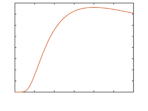
In figure 1 we compare the present (8.1) with the spontaneous speed predicted by Hu et al. (Reference Hu, Lin, Rafai and Misbah2019), who took $R=200$. For that value, $2/{\ln R}$ is roughly $0.4$. The critical Péclet number found by Hu et al. (Reference Hu, Lin, Rafai and Misbah2019), ${\approx }0.466$, is indeed close to that value. For larger ${{Pe}}$, we observe in figure 1 an interval where the present (8.1) and the prediction of Hu et al. (Reference Hu, Lin, Rafai and Misbah2019) are virtually indistinguishable. (While the present approximation is strictly valid for ${{Pe}}\ll 1$, it is remarkably accurate up to about ${{Pe}}=1$.) When ${{Pe}}$ is larger still, the small-${{Pe}}$ approximation (8.1) becomes irrelevant, and the two predictions separate off.

Figure 1.

Spontaneous speed as a function of ${{Pe}}$. The solid curve is the present (8.1). The dashed curve represents the straight-motion speed displayed in figure 1 of Hu et al. (Reference Hu, Lin, Rafai and Misbah2019).

9. Concluding remarks

Given the absence of a reference stationary state, the concept of a critical ${{Pe}}$ in 2-D unbounded domains becomes vague. This is corroborated by the numerical predictions (Hu et al. Reference Hu, Lin, Rafai and Misbah2019) of a critical Péclet number that diminishes slowly to zero as the distance to the remote boundary is enlarged. The prediction of a critical Péclet number, based upon a linear stability analysis, is accordingly irrelevant for the unbounded problem. Moreover, the nonlinear advection–diffusion problem governing spontaneous motion is expected to be well posed in the unbounded configuration for any finite ${{Pe}}$.

We therefore advocate for the use of unbounded domains in theoretical investigations of 2-D spontaneous motion, mimicking the idealised configurations studied in three dimensions. Adopting this conceptual approach, we have addressed herein the unbounded problem from the outset. Our work reveals that spontaneous motion occurs for arbitrarily small Péclet numbers. This is fundamentally different from the 3-D case (Michelin et al. Reference Michelin, Lauga and Bartolo2013).

The present analysis may be extended to incorporate more realistic descriptions of interfacial activity, where the prescribed flux is replaced by a first-order kinetic model (Ebbens et al. Reference Ebbens, Tu, Howse and Golestanian2012; Li Reference Li2022). Since that model still gives rise to a logarithmic divergence with distance in a 2-D diffusive transport (Yariv Reference Yariv2017; Yariv & Crowdy Reference Yariv and Crowdy2020; Saha & Yariv Reference Saha and Yariv2022), the stationary state remains ill posed. It is therefore anticipated that, even with a more realistic interfacial description, spontaneous motion emerges at arbitrarily small Péclet numbers.