


Impact Statement
Although ocean currents play a crucial role in regulating Earth’s climate and in the dispersal of marine species and pollutants, such as microplastics, they are difficult to measure accurately. Satellite observations offer the only means by which ocean currents can be estimated across the entire global ocean. However, these estimates are severely contaminated by noise. Removal of this noise by conventional filtering methods leads to blurred currents. Therefore, this work presents a novel deep-learning method that successfully removes noise, while greatly reducing the current attenuation, allowing more accurate estimates of current speed and position to be determined. The method may have more general applicability to other geophysical observations where filtering is required to remove noise.
1. Introduction
Ocean currents play an important role in Earth’s climate system, transporting vast quantities of heat from the tropics to higher latitudes, thereby helping to maintain Earth’s heat balance (Talley, Reference Talley2013). In so doing, ocean currents can significantly impact global climate patterns and local weather conditions (Broecker, Reference Broecker1998; Sutton and Hodson, Reference Sutton and Hodson2005; Zhang and Delworth, Reference Zhang and Delworth2006). Rates and patterns of ocean heat (Winton et al., Reference Winton, Griffies, Samuels, Sarmiento and Frölicher2013; Bronselaer and Zanna, Reference Bronselaer and Zanna2020) and carbon dioxide (Le Quéré et al., Reference Le Quéré, Raupach, Canadell, Marland, Bopp, Ciais, Conway, Doney, Feely, Foster, Friedlingstein, Gurney, Houghton, House, Huntingford, Levy, Lomas, Majkut, Metzl, Ometto, Peters, Prentice, Randerson, Running, Sarmiento, Schuster, Sitch, Takahashi, Viovy, van der Werf and Woodward2009; Sallée et al., Reference Sallée, Matear, Rintoul and and Lenton2012) storage are strongly influenced by the ocean circulation; for example, changes in circulation of the North Atlantic brought on by anthropogenic warming play a critical role in regulating the overall climatic response (Winton et al., Reference Winton, Griffies, Samuels, Sarmiento and Frölicher2013; Marshall et al., Reference Marshall, Scott, Armour, Campin, Kelley and Romanou2015). Ocean current transports are also of critical importance to marine life, carrying essential nutrients and food to marine ecosystems while distributing larvae and reproductive cells (Merino and Monreal-Gómez, Reference Merino and Monreal-Gómez2009). Ocean currents also act as a global dispersal mechanism for pollutants such as mircoplastics (van Duinen et al., Reference van Duinen, Kaandorp and van Sebille2022; Ypma et al., Reference Ypma, Bohte, Forryan, Naveira Garabato, Donnelly and van Sebille2022), and those arising from power generation, industry, and other human activities (Doglioli et al., Reference Doglioli, Magaldi, Vezzulli and Tucci2004; Buesseler et al., Reference Buesseler, Aoyama and Fukasawa2011; Goni et al., Reference Goni, Trinanes, MacFadyen, Streett, Olascoaga, Imhoff, Muller-Karger and Roffer2015). Finally, ocean currents affect shipping and fishing industries, with consequences for safe and efficient navigation (Singh et al., Reference Singh, Sharma, Sutton, Hatton and Khan2018). For these reasons, all of which have profound implications for society, accurate measurements of the global ocean’s surface currents are vitally important.
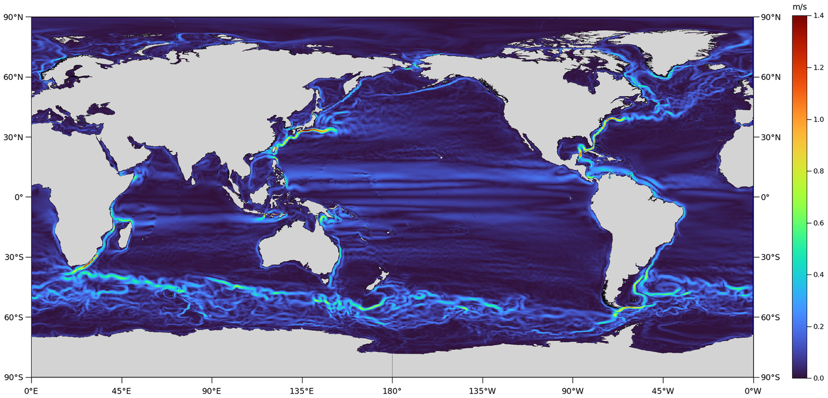
While ocean currents may be measured by deploying in-situ current meters, either moored or free-floating, their sampling is rather too sparse in time and space to obtain a consistently accurate estimate of the ocean’s circulation over the entire global ocean (Zhou et al., Reference Zhou, Paduan and Niiler2000; Poulain et al., Reference Poulain, Menna and Mauri2012). We can, however, exploit the fact that the ocean is largely in geostrophic balance to calculate the ocean’s surface circulation from observations of its time-mean dynamic topography (MDT). The surface geostrophic current velocities shown in Figure 1 are computed from the MDT generated by a high-resolution climate model, where the MDT is simply the time-averaged sea surface height fields generated by the model. The actual ocean’s MDT describes the deviation of the time-mean sea surface (MSS) from the marine geoid, defined as the shape the oceans would take if affected by gravity and rotation alone (corresponding to zero sea surface height in the model.) The MDT, therefore, represents the influence of momentum, heat, and freshwater (buoyancy) fluxes between the ocean and the atmosphere.
Surface geostrophic current velocity map computed from the high-resolution CMCC-CM2-HR4 climate model (Scoccimarro et al., Reference Scoccimarro, Bellucci and Peano2019) prepared for Coupled Model Intercomparison Project Phase 6 (CMIP6).
Observationally, the MDT can be determined geodetically by subtracting a geoid height surface from an altimetric MSS:
 $$ \eta \left(\theta, \phi \right)=H\left(\theta, \phi \right)-N\left(\theta, \phi \right), $$
where $ \eta $
,
$ \eta $
, $ H $
and
$ H $
and $ N $
represent the MDT, the MSS and the geoid height (resp.), with
$ N $
represent the MDT, the MSS and the geoid height (resp.), with $ \theta $
and
$ \theta $
and $ \phi $
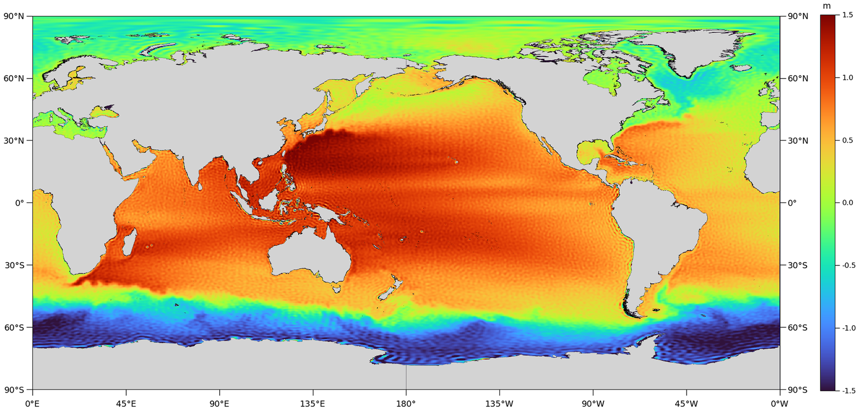
representing latitude and longitude (resp.). As described in Bingham et al. (Reference Bingham, Haines and Hughes2008), the simplicity of Equation 1 belies many challenges that arise in practice because of the fundamentally different nature of the geoid and the MSS and the approaches by which they are determined. As a result, observed MDTs contain unphysical noise patterns that appear as striations and orange skin-like features (Figure 2), the origin of which is discussed below.
$ \phi $
representing latitude and longitude (resp.). As described in Bingham et al. (Reference Bingham, Haines and Hughes2008), the simplicity of Equation 1 belies many challenges that arise in practice because of the fundamentally different nature of the geoid and the MSS and the approaches by which they are determined. As a result, observed MDTs contain unphysical noise patterns that appear as striations and orange skin-like features (Figure 2), the origin of which is discussed below.
DTU18-EIGEN-6C4 MDT, expanded up to degree/order 280.
Assuming geostrophic balance, the ocean’s steady-state circulation is proportional to the direction and magnitude of the MDT gradients (Knudsen et al., Reference Knudsen, Bingham, Andersen and Rio2011). Thus, the zonal and meridional surface geostrophic currents, u and v (resp.), are calculated by
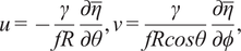 $$ u=-\frac{\gamma }{fR}\frac{\partial \overline{\eta}}{\partial \theta },v=\frac{\gamma }{fR cos\theta}\frac{\partial \overline{\eta}}{\partial \phi }, $$
where $ \theta $
is latitude and
$ \theta $
is latitude and $ \phi $
is longitude;
$ \phi $
is longitude; $ \gamma $
denotes the normal gravity;
$ \gamma $
denotes the normal gravity; $ R $
denotes the Earth’s mean radius; and finally
$ R $
denotes the Earth’s mean radius; and finally $ f=2{\omega}_e sin\theta $
is the Coriolis parameter, in which
$ f=2{\omega}_e sin\theta $
is the Coriolis parameter, in which $ {\omega}_e $
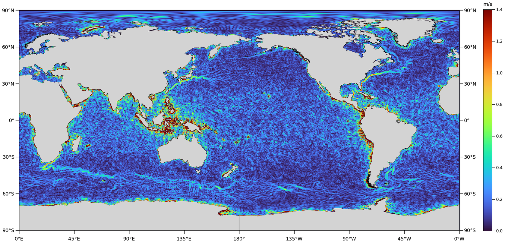
denotes the Earth’s angular velocity. Because the surface geostrophic currents are calculated as the gradient of the MDT (Equation 2), the noise in the latter surface is amplified when the currents are calculated, thus obscuring the signal we seek (Figure 3). Noise is present over the entirety of the ocean’s global surface. However, due to steep gradients in the gravity field adjacent to some coastlines, such as along the west coast of South America, around the Caribbean, and in the Indonesian through-flow region, noise here is particularly severe; a problem exacerbated towards the equator where the
$ {\omega}_e $
denotes the Earth’s angular velocity. Because the surface geostrophic currents are calculated as the gradient of the MDT (Equation 2), the noise in the latter surface is amplified when the currents are calculated, thus obscuring the signal we seek (Figure 3). Noise is present over the entirety of the ocean’s global surface. However, due to steep gradients in the gravity field adjacent to some coastlines, such as along the west coast of South America, around the Caribbean, and in the Indonesian through-flow region, noise here is particularly severe; a problem exacerbated towards the equator where the $ 1/f $
factor in the geostrophic equations approaches zero. This poses a particular challenge to conventional filters.
$ 1/f $
factor in the geostrophic equations approaches zero. This poses a particular challenge to conventional filters.
Surface geostrophic current velocity map computed from the DTU18-EIGEN-6C4 MDT expanded up to degree/order 280, via Equation 2, in which $ f=2{\omega}_e sin\theta $
; however, for
$ f=2{\omega}_e sin\theta $
; however, for $ \theta <{15}^{\circ } $
from the equator, we fix
$ \theta <{15}^{\circ } $
from the equator, we fix $ f=2{\omega}_e\mathit{\sin}(15) $
to avoid the singularity within this region.
$ f=2{\omega}_e\mathit{\sin}(15) $
to avoid the singularity within this region.
The fundamental issue with determining the MDT and associated currents geodetically is that the MSS can be obtained at a much higher spatial resolution than the geoid. The MSS is defined naturally on a high resolution (up to 1 arc minute) geographical grid, while the Earth’s gravity field is expressed naturally as a truncated set of spherical harmonics up to a max degree and order (d/o) $ {L}_{\mathrm{max}} $
, from which a gridded geoid height surface can be calculated with a spatial resolution of
$ {L}_{\mathrm{max}} $
, from which a gridded geoid height surface can be calculated with a spatial resolution of $ \sim $
20000/
$ \sim $
20000/ $ L $
km, where
$ L $
km, where $ L\le {L}_{\mathrm{max}} $
. The geoid fails to capture higher resolution features of Earth’s gravity field that are present in the MSS. Therefore, unless steps are taken to address the problem (see below), when the geoid is subtracted from the MSS, the MDT will contain geodetic features unrelated to the ocean’s circulation. When computing the geoid, we may truncate the spherical harmonic expansion at some d/o
$ L\le {L}_{\mathrm{max}} $
. The geoid fails to capture higher resolution features of Earth’s gravity field that are present in the MSS. Therefore, unless steps are taken to address the problem (see below), when the geoid is subtracted from the MSS, the MDT will contain geodetic features unrelated to the ocean’s circulation. When computing the geoid, we may truncate the spherical harmonic expansion at some d/o $ L\le {L}_{\mathrm{max}} $
. The missing geoid signal for d/o
$ L\le {L}_{\mathrm{max}} $
. The missing geoid signal for d/o $ >L $
is known as the geoid omission error. Since much of this omission error, or missing geodetic signal, is present in the higher resolution MSS, it remains in the MDT. Truncation of the spherical harmonic series introduces an additional error in the geoid, and therefore in the MDT, in the form of Gibbs fringes, which radiate away from regions of strong gradient in the gravity field (Bingham et al., Reference Bingham, Haines and Hughes2008). This can be thought of as a non-local, artifactual geoid omission error.
$ >L $
is known as the geoid omission error. Since much of this omission error, or missing geodetic signal, is present in the higher resolution MSS, it remains in the MDT. Truncation of the spherical harmonic series introduces an additional error in the geoid, and therefore in the MDT, in the form of Gibbs fringes, which radiate away from regions of strong gradient in the gravity field (Bingham et al., Reference Bingham, Haines and Hughes2008). This can be thought of as a non-local, artifactual geoid omission error.
Geoid omission error can be reduced by computing the geoid to $ {L}_{\mathrm{max}} $
. However, apart from the missing signal, the spherical harmonic coefficients that are used to calculate the geoid include errors that grow exponentially with increasing d/o (reflecting the challenge of measuring Earth’s gravity at ever finer spatial scales). The error in the geoid, and therefore the MDT, due to the error in the terms included in the spherical harmonic expansion to d/o
$ {L}_{\mathrm{max}} $
. However, apart from the missing signal, the spherical harmonic coefficients that are used to calculate the geoid include errors that grow exponentially with increasing d/o (reflecting the challenge of measuring Earth’s gravity at ever finer spatial scales). The error in the geoid, and therefore the MDT, due to the error in the terms included in the spherical harmonic expansion to d/o $ L\le {L}_{\mathrm{max}} $
is referred to as the geoid commission error. Depending on the error characteristics of the geoid used, at some d/o
$ L\le {L}_{\mathrm{max}} $
is referred to as the geoid commission error. Depending on the error characteristics of the geoid used, at some d/o $ L<{L}_{\mathrm{max}} $
, the reduction in geoid omission error may be outweighed by the growth in geoid commission error. Finally, MSS error will also make a small contribution to the total error budget of the MDT.
$ L<{L}_{\mathrm{max}} $
, the reduction in geoid omission error may be outweighed by the growth in geoid commission error. Finally, MSS error will also make a small contribution to the total error budget of the MDT.
Regardless of the origin, the issue of MDT noise is exacerbated by the fact that the amplitude of the MDT is of order 1 m, while the amplitude of the geoid and MSS is of the order 100 m. Thus, it only takes a small (1%) error in either of the constituent surfaces to produce an error in the MDT of the same magnitude as the MDT itself.
While methods have been developed to reduce the impact of geoid omission error (Bingham et al., Reference Bingham, Haines and Hughes2008), it is still necessary to filter the MDT to remove residual omission error and commission error (Figure 3). This can be achieved by applying a simple linear filter (e.g., Gaussian (Bingham et al., Reference Bingham, Haines and Hughes2008), Hamming (Jayne, Reference Jayne2006)) directly to the MDT before calculating current velocities. However, in addition to removing noise, such filters attenuate steep MDT gradients, leading to blurred and decreased geostrophic current velocities.
More complex filters have been designed to minimize attenuation by accounting for strong gradients. For example, Bingham (Reference Bingham2010) employed a nonlinear anisotropic diffusive filtering approach and Sánchez-Reales et al. (Reference Sánchez-Reales, Andersen and Vigo2016) presented an edge-enhancing diffusion approach. Despite improving on traditional approaches, such filters come with their own problems. In particular, they depend on arbitrary functions and parameters controlling their sensitivity to gradients. This can lead to over-sharpening of steep gradients that exaggerate oceanographic features or directional bias that causes strong currents to have a staircase-like effect in the associated surface geostrophic current maps. Hence, there remains a need to develop a more sophisticated filtering method that can remove noise effectively while minimizing attenuation of steeper gradients, thereby maximizing the amount of oceanographic information obtained from the geodetic MDT.
In this study, we implement a supervised machine learning approach to directly filter the geodetic surface geostrophic current maps, allowing us to guide the network to learn a denoising transformation that accurately removes geodetic noise while preserving oceanographic features. This approach requires training pairs, each consisting of a noisy (corrupted) input and a clean target, to train the denoiser. Since we cannot obtain a geodetic current field free from noise without filtering, and filtering has undesirable consequences (the problem we are trying to address), the training pairs must be found elsewhere. Therefore, we construct training pairs for supervised learning by adding synthesized noise to a naturally smooth target current field possessing similar characteristics to that of our desired output, that is, produced by numerical models. Using these pairs, we then train a Convolutional Denoising Auto-Encoder (CDAE) to remove the noise from the current field. The autoencoder network has proven to be effective in the region of image denoising (Vincent et al., Reference Vincent, Larochelle, Lajoie, Bengio, Manzagol and Bottou2010; Xie et al., Reference Xie, Xu and Chen2012; Lore et al., Reference Lore, Akintayo and Sarkar2017), outperforming conventional denoising methods due to the ability of neural networks to learn non-linear patterns. It should, therefore, be able to distinguish between actual currents and the contaminating noise. Finally, we apply the trained CDAE to remove the noise from currents obtained from a geodetic MDT. This work will focus on four key regions containing major currents: the Gulf Stream in the North Atlantic; the Kuroshio Current in the North Pacific; the Agulhas Current in the Indian Ocean; and the Brazil and Malvinas Currents in the South Atlantic, hereafter referred to as the Brazil-Malvinas Confluence Zone (BMCZ). These four regions have been chosen as they each play an important role in the global ocean’s circulation, but vary in terms of complexity and current strength, and thus the signal to noise ratio. They therefore represent a strong test of the method’s versatility and general applicability.
This paper is organized as follows. In Section 2, we describe our approach to generating synthetic noise and training pairs. Here we introduce the data used in this study. Section 3 describes the architecture and training set-up of the denoising network. Section 4 presents the denoising results of the trained CDAE network applied to real-world geodetic geostrophic currents and its performance is compared against conventional filtering. Finally, Section 5 provides a concluding discussion.
2. Generating Training Pairs
In this paper, we implement a blind image denoising method using deep learning, for which we require training pairs. In the case of image denoising, training pairs refers to the pairings of noisy and corresponding clean example images, from which the CDAE can learn a denoising transformation. In our case, the true noise-free field (or ground-truth as it is referred to in the machine learning literature) does not exist. A commonly used strategy in computer vision to overcome a lack of training pairs is to apply synthesized noise to a dataset of analogous, but naturally smooth targets (Chen et al., Reference Chen, Chen, Chao and Yang2018). By learning the mapping between synthesized noisy inputs and noise-free targets, the model is able to learn a denoising transformation by which similar types of noise can be removed from new images. Therefore, the model is able to generalize towards new data.
2.1. Clean target data
In order to generate training pairs for a case where a noise-free field does not exist, we first require a dataset of analogous, naturally noise-free images possessing characteristics similar to those we wish to denoise to which we can add synthetic noise. For this purpose, we compute surface geostrophic current velocity maps from a set of ocean model MDTs, as in Figure 1, to be used as noise-free training targets. Ocean model data is a suitable choice as it contains the types of oceanographic features we wish to preserve during noise-removal while being free from the noise that contaminates geodetic MDTs.
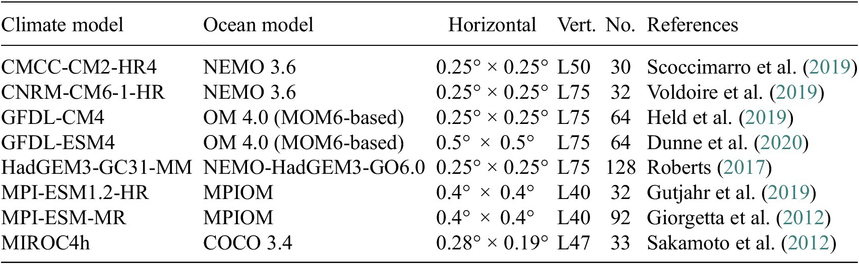
The ocean components of several global climate models from the Coupled Model Intercomparison Project (CMIP)Footnote 1 provide the target data for this study. Utilizing the CMIP data provides a large dataset of naturally smooth MDTs, containing the same types of oceanographic features we wish to retrieve from the geodetic data through denoising. We use the historical simulations from a set of CMIP5 and CMIP6 models (Table 1) spanning the period 1850-2006. As lower resolution models may not sufficiently resolve key oceanographic features that are needed for training, such as the Gulf Stream, only models whose ocean component has a horizontal resolution $ \le $
1/2° are chosen (corresponding to approximately
$ \le $
1/2° are chosen (corresponding to approximately $ L $
=360). All products are computed as 5-year means of SSH and are interpolated to a common 1/4° grid, resulting in 473 global maps in total. The surface geostrophic currents are then calculated according to Equation 2.
$ L $
=360). All products are computed as 5-year means of SSH and are interpolated to a common 1/4° grid, resulting in 473 global maps in total. The surface geostrophic currents are then calculated according to Equation 2.
Climate model data used in this study; native horizontal resolution expressed as latitude $ \times $
longitude (is approximate); number of vertical levels; total number of MDTs generated by each model across all ensembles; and key reference.
$ \times $
longitude (is approximate); number of vertical levels; total number of MDTs generated by each model across all ensembles; and key reference.
2.2. Generating synthesized noise using generative networks
The second component required for generating training pairs where suitable noise-free images do not exist is a synthesized noise model with which to artificially contaminate the naturally smooth images discussed in the previous section (2.1). A straightforward approach is to assume a Gaussian noise model (e.g., Zhang et al., Reference Zhang, Zuo, Chen, Meng and Zhang2017a,Reference Zhang, Zuo, Gu and Zhangb). However, a Gaussian noise model is unlikely to provide a good representation of the type of noise present in the natural images, which generally exhibit non-homogeneous complex patterns. This is important as it has been shown that training denoising models using more realistic synthesized noise allows the learned denoising transformation to generalize better towards real data (Chen et al., Reference Chen, Chen, Chao and Yang2018). This is particularly the case for geostrophic currents produced from geodetic MDTs (Figure 3) which suffer from non-linear structural noise. Thus, there is a clear motivation to develop a realistic noise model that achieves a good approximation of real geodetic noise.
Since noise can be considered to be an image, we employ a deep generative convolutional network to create a realistic noise model that creates images emulating the type of noise present in the geodetic current maps, that is, the type of noise we wish to remove. (To the best knowledge of the authors, this is the first time deep learning has been used to replicate the geodetic noise present in geodetically-determined geostrophic surface currents.) Generative networks aim to learn the ‘true’ underlying statistical distribution of a given dataset in order to generate new synthetic data that could plausibly have been drawn from said dataset. Such networks use unsupervised learning, and thus do not require a dataset of labeled targets. However, performance evaluation is less straightforward than that of supervised learning methods, usually being indirect or qualitative. Therefore, we investigate the efficacy of multiple deep generative networks for the task of synthesized noise generation, and perform a comparative analysis to select the desired noise model (Section 2.5).
The noise-generating networks employed in this investigation include a Deep Convolutional Generative Adversarial Network (DCGAN) (Goodfellow et al., Reference Goodfellow, Pouget-Abadie, Mirza, Xu, Warde-Farley, Ozair, Courville and Bengio2014; Radford et al., Reference Radford, Metz and Chintala2015), a Variational Autoencoder (VAE) (Kingma and Welling, Reference Kingma and Welling2013) and a Wasserstein Autoencoder (WAE) (Tolstikhin et al., Reference Tolstikhin, Bousquet, Gelly and Schoelkopf2017). GANs are derived from a game theory scenario where two sub-models compete against, and thus learn from, one another (Goodfellow et al., Reference Goodfellow, Pouget-Abadie, Mirza, Xu, Warde-Farley, Ozair, Courville and Bengio2014). In the ideal equilibrium scenario the discriminator learns to identify real samples from generated ones and the generator will learn to produce images that can fool the discriminator. GANs tend to learn a variety of non-linear patterns well and thus have been shown to reproduce highly realistic images. However, the method of training, that is, reaching an equilibrium rather than an optimum, can be unstable (El-Kaddoury et al., Reference El-Kaddoury, Mahmoudi and Himmi2019). VAEs extend the autoencoder (Vincent et al., Reference Vincent, Larochelle, Lajoie, Bengio, Manzagol and Bottou2010) to enable generation of new data by introducing regularity to the distribution over the latent space from which new data samples can be drawn (Cai et al., Reference Cai, Gao and Ji2019). This regularization can prevent the generation of samples that clearly lie outside the target distribution. However, the smooth assumption of the latent space may also restrict the VAE network from sufficiently learning the distribution of some target datasets. The WAE, a modified VAE whose encoded distribution is forced to form a continuous mixture matching the prior distribution, rather than matching a single sample, is included in this investigation as it has been shown to produce better-quality images compared to the standard VAE in some cases (Tolstikhin et al., Reference Tolstikhin, Bousquet, Gelly and Schoelkopf2017).
2.3. Using geodetic data to train generative networks
To reliably generate a realistic estimate of the noise distribution, the noise-generating networks must be provided with a set of training samples that represent the noise patterns well. For this, we utilize unfiltered geodetic geostrophic velocities, that is, the data we wish to denoise, so that the networks can learn as close a representation to the real noise as possible.
The surface geostrophic velocities used for synthesized noise generation are computed from a set of geodetic MDTs, calculated by the spectral approach (Bingham et al., Reference Bingham, Haines and Hughes2008) via Equation 1. The global gravity models used to generate the set of geodetic MDTs used in this study are listed in Table 2, all of which are available at the International Centre for Global Earth Models (ICGEM) web portal (Ince et al., Reference Ince, Barthelmes, Reißland, Elger, Förste, Flechtner and Schuh2019). Said geoids are derived from a combination of satellite gravity field missions: GOCE (Drinkwater et al., Reference Drinkwater, Floberghagen, Haagmans, Muzi and Popescu2003), GRACE (Tapley et al., Reference Tapley, Bettadpur, Watkins and Reigber2004), surface data and altimetry data. Each geoid is expanded up to a common d/o $ L $
=280 before MDT calculation, to ensure noise patterns (which change with varying
$ L $
=280 before MDT calculation, to ensure noise patterns (which change with varying $ L $
) remain consistent across the training dataset. We utilize a recent global high resolution MSS product published by the Danish National Space Institute (DTU), termed the DTU18 MSS (Andersen et al., Reference Andersen, Knudsen and Stenseng2018), for each MDT calculation. The DTU18 MSS is calculated from 20 years of altimetry data, over the period 1993-2012, with a spatial resolution of 1 arc minute. The spectrally truncated MSS, which is transformed from the gridded product to a set of spherical harmonic coefficients, is expanded up to the same degree/order
$ L $
) remain consistent across the training dataset. We utilize a recent global high resolution MSS product published by the Danish National Space Institute (DTU), termed the DTU18 MSS (Andersen et al., Reference Andersen, Knudsen and Stenseng2018), for each MDT calculation. The DTU18 MSS is calculated from 20 years of altimetry data, over the period 1993-2012, with a spatial resolution of 1 arc minute. The spectrally truncated MSS, which is transformed from the gridded product to a set of spherical harmonic coefficients, is expanded up to the same degree/order $ L $
as the geoid. This ensures that both local and non-local omission errors in the geoid are closely matched in the MSS and are thus minimized.
$ L $
as the geoid. This ensures that both local and non-local omission errors in the geoid are closely matched in the MSS and are thus minimized.
The gravity field models used for synthesized noise generation; year published; maximum spherical harmonic degree (later expanded up to the same degree/order of 280 across models); data source; and key reference.
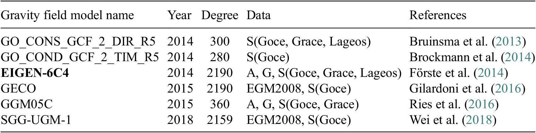
Note. The data column summarizes the datasets used in the development of each model, where A is for altimetry, S is for satellite and is G for ground data (e.g., terrestrial, shipborne and airborne measurements). The model in bold text is used to generate the DTU18_EIGEN-6C4 MDT which is filtered in final analysis of Section 4.2.
A potential issue with using unfiltered geodetic current fields to train the noise generating networks is that these fields contain both the noise we later wish to remove and the current that we wish to preserve. Thus, the networks may learn a distribution that mixes both the noise and some current signal. This would result in creating synthetic noise patterns that also contain oceanographic features. To avoid this, the global maps are split into small regions where large-scale oceanographic structures are not prominent. These smaller regions (hereafter referred to as tiles) must be large enough to capture a significant portion of the geodetic noise patterns, but small enough to prevent capturing significant long-range oceanographic features. This ensures that, after randomizing the order of the tiles, the long-range oceanographic features are obfuscated, making the generative network more likely to learn the consistent distribution of the geodetic noise. Through visual investigation it was found that a tile size of $ 32\times 32 $
pixels (8
$ 32\times 32 $
pixels (8 $ {}^{\circ}\times {8}^{\circ } $
) was the largest suitable size for training across all generative networks, and hence is used for all following experiments in this section; at larger sizes, higher frequency noise patterns were not reproduced and generative networks learned to focus on the more basic filamentary structures of the currents, which is undesirable. Furthermore, in this study tiles at high latitudes (above 64°N and below 64°S) are discarded to avoid the distortion which becomes increasingly severe on a standard equidistant cylindrical projection towards the poles. This provides a consistent noise pattern distribution. Therefore, care has to be taken when applying the denoising network at latitudes above or below this cutoff, as the denoising network has not been exposed to such projection distortions.
$ {}^{\circ}\times {8}^{\circ } $
) was the largest suitable size for training across all generative networks, and hence is used for all following experiments in this section; at larger sizes, higher frequency noise patterns were not reproduced and generative networks learned to focus on the more basic filamentary structures of the currents, which is undesirable. Furthermore, in this study tiles at high latitudes (above 64°N and below 64°S) are discarded to avoid the distortion which becomes increasingly severe on a standard equidistant cylindrical projection towards the poles. This provides a consistent noise pattern distribution. Therefore, care has to be taken when applying the denoising network at latitudes above or below this cutoff, as the denoising network has not been exposed to such projection distortions.
2.4. Generative network architecture and training details
2.4.1. VAE
The VAE’s encoder has five 3x3 convolutional blocks, with 32, 64, 128, 256 and 512 output channels. Similarly, the decoder has five 3x3 deconvolutional blocks, with 512, 256, 128, 64, and 32 output channels, which upsample the encoded features. Each convolutional and deconvolutional layer is followed by a Leaky rectified linear unit (ReLU). The final layer uses the tanh activation function. We use the loss adaption presented by (Higgins et al., Reference Higgins, Matthey, Pal, Burgess, Glorot, Botvinick, Mohamed and Lerchner2017), where the Kullback-Leibler (KL) divergence loss is scaled using a parameter $ \beta $
. In our case, we found that
$ \beta $
. In our case, we found that $ \beta $
=0.01 provided stable results.
$ \beta $
=0.01 provided stable results.
2.4.2. WAE
For the WAE, the encoder-decoder setup is the same as for the VAE. However, the Wasserstein distance replaces the reconstruction error used in VAEs, and, rather than KL divergence, the maximum mean discrepancy (MMD) is used as the regularization penalty (Gretton et al., Reference Gretton, Borgwardt, Rasch, Scholkopf and Smola2012). Following the best training configuration from the original WAE paper (Tolstikhin et al., Reference Tolstikhin, Bousquet, Gelly and Schoelkopf2017), the MMD-based penalty is computed with the inverse multi-quadratics kernel (IMQ).
2.4.3. DCGAN
The generator of the DCGAN consists of two 3x3 convolutional blocks, with 128 and 64 output channels, each followed by a ReLU activation function. The hyperbolic tangent function (tanh) is used as the activation function for the final output layer of the generator. The discriminator consists of four 3 x 3 convolutional blocks, with 16, 32, 64, and 128 output channels, followed by a fully connected layer that uses the Sigmoid activation function to generate a binary prediction. Binary Cross Entropy (BCE) is used for the adversarial loss function.
2.4.4. Training process
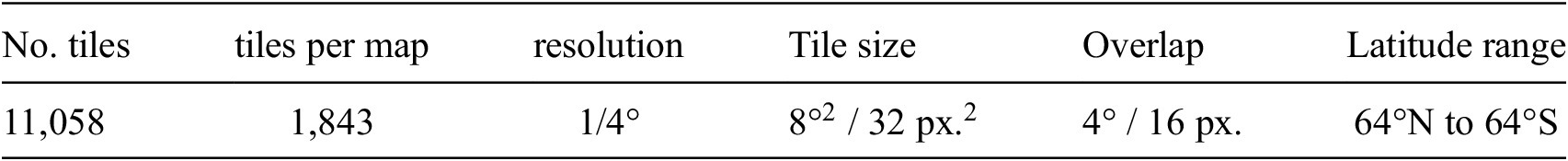
All generative networks are trained over 300 epochs (an epoch involves training the network over the whole training dataset exactly once) using the Adam optimizer (Kingma and Ba, Reference Kingma and Ba2014) on a dataset of 11,058 tiles from a set of six geodetic geostrophic current maps, with each global map split into 1,843 tiles overlapping by 16 pixels (4°). We use a batch size of 512, and set the learning rate to 0.005. The properties of the generative network training dataset are summarized in Table 3.
Details of the generative network training data constructed from a set of Gravity field models (Table 2) and the DTU18 MSS.
2.5. Synthesized noise generation results
In this section, we present the synthesized noise generation results from the three generative networks discussed in Section 2.2. Subsequently, we provide a qualitative discussion, we perform a comparative Fourier analysis on the noise model produced by each trained generative network, and we compute a similarity metric between the spectral distributions of real and synthetic tiles to provide a quantitative estimate of the noise quality, from which the most suitable synthesized noise model is determined.
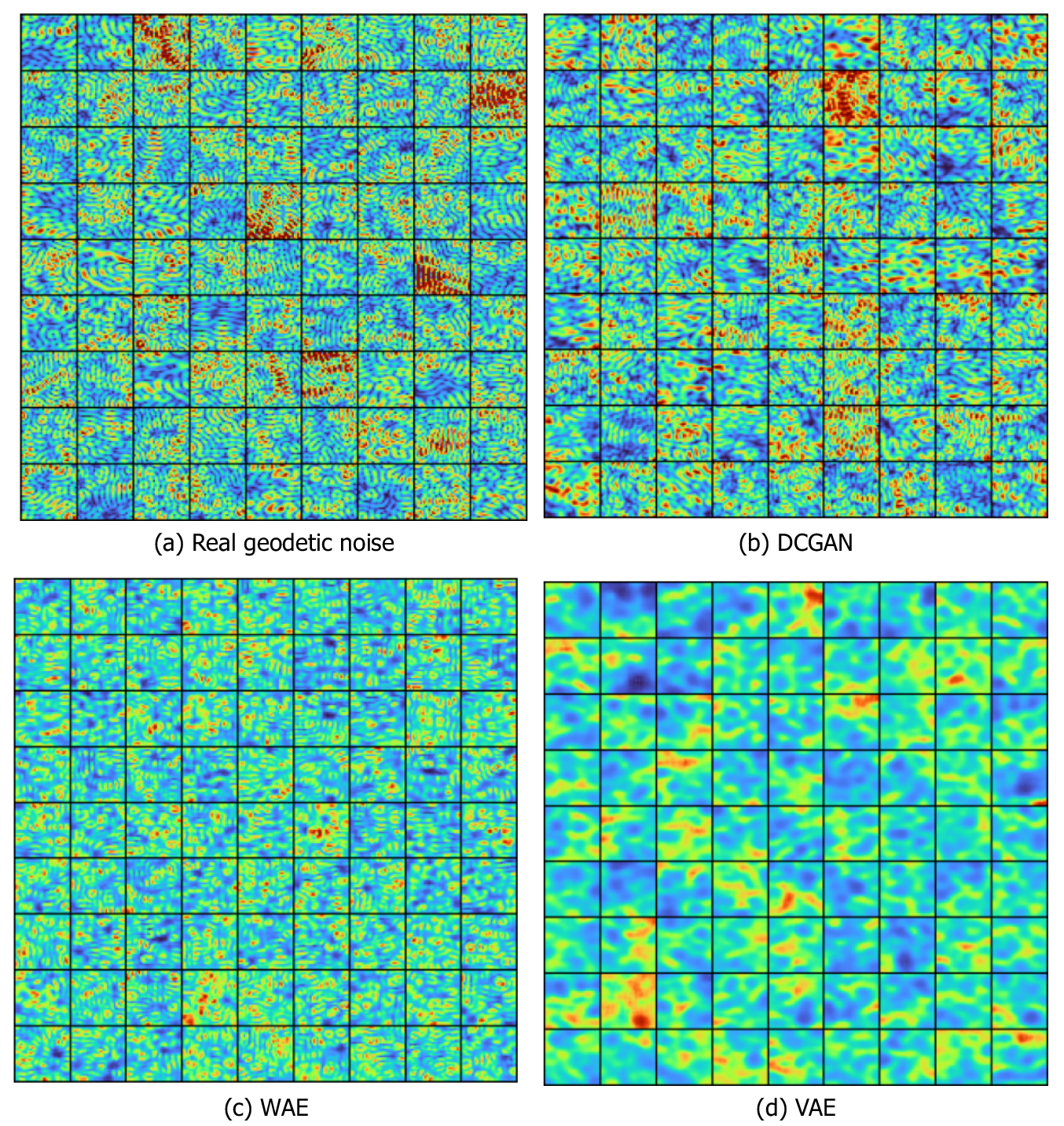
We present the real geodetic noise tiles in Figure 4a, which provide a baseline for comparison of noise properties such as patterns, structure, color intensity and variability. The DCGAN tiles exhibit the most realistic looking noise (Figure 4b) with a suitable variation in both frequency and amplitude, matching similar properties in the real geodetic noise. It can be seen that the WAE network produces slightly less realistic samples in comparison to the DCGAN. However, the network does exhibit small scale circular structures which resemble those present in the real geodetic noise (Figure 4c). The WAE tiles have a consistent distribution across all tiles. Due to this, there is less variation in both intensity and structure, which we would expect from real geodetic noise. Furthermore, the structures generated by the WAE exhibit grid-like structures along the Cartesian axes. In contrast, the DCGAN noise has more realistic variation. The VAE generates significantly less realistic outputs, producing blurry shapes with some filamentary features (Figure 4d) and fails to capture any fine grain detail. These filamentary structures more closely resemble general oceanographic features such as currents over the small circular patterns of the geodetic noise. This is likely due to the inherent nature of VAEs, which tend to prioritize general shape rather than finer structural features (Zhao et al., Reference Zhao, Song and Ermon2017), and the lack of constraint on the learned latent space representation.
Generated noise tiles from real geodetic data and synthesized data from generative networks.
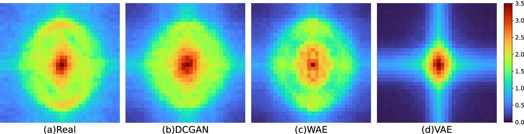
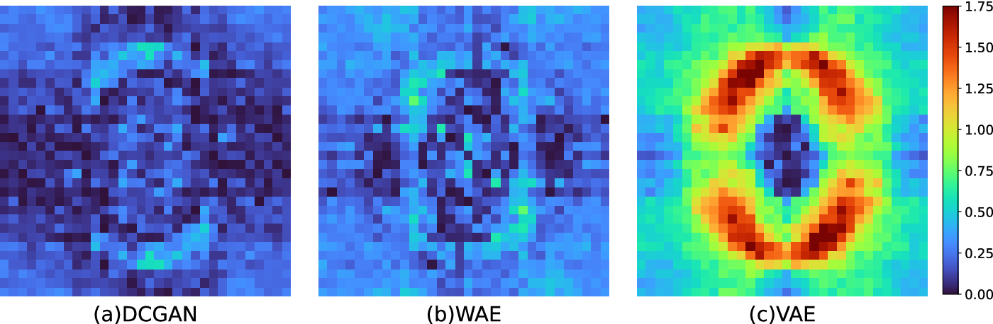
We compute the fast Fourier transform (FFT) from a batch of 50 randomly chosen tiles from the training dataset of real geodetic data and from each synthesized noise model. Figure 5 shows the shifted log magnitude of the FFT spectrum for each batch, in which lower frequencies are represented at the center, and Figure 6 shows the corresponding difference in magnitude spectra between the training data and each synthesized noise model. The residual difference of the VAE differs by the greatest margin, managing to reproduce a similar distribution at low frequencies, but failing quite severely at the mid-range. In contrast, residual differences computed for the DCGAN and WAE exhibit relatively low residual differences across the full spectrum (Figure 6). However, the DCGAN is superior to the WAE across mid and high frequencies.
The 2D FFT magnitude spectra computed across a batch of 50 tiles.
The difference between real geodetic noise and synthesized noise in terms of FFT magnitude spectra.
To provide a similarity index between the real and the synthetic data we compute the KL divergence (Hershey and Olsen, Reference Hershey and Olsen2007), which measures the dissimilarity between two probability distributions, on the radial profile of the FFT magnitude spectra. The KL divergence scores for the VAE, WAE, and DCGAN are 0.1422, 0.0350, and 0.0047 (resp.). The best (lowest) score is achieved by the DCGAN, reinforcing the conclusions drawn from the qualitative analyses of the noise patterns and of their Fourier transforms, athus providing confidence that the DCGAN generated noise best represents the real geodetic noise.
We can conclude, therefore, that the DCGAN generates the highest quality distribution according to the above analysis, reproducing similar magnitudes in the full frequency range, and is thus the most suitable choice for a realistic synthesized noise model. Furthermore, the efficacy of using this approach to generate synthetic noise is indirectly evaluated in Section 4 by assessing the ability of a denoiser, trained on said noise, to remove real noise.
2.6. Quilting
An implication of the proposed synthesized noise generation method is that the generative networks are trained on and thus output tiles smaller in scale than significant current features ( $ 32\times 32 $
pixels or 8
$ 32\times 32 $
pixels or 8 $ {}^{\circ}\times {8}^{\circ } $
). In contrast to the generative networks, we wish to train a denoising network on larger regions, regions large enough to retain entire current structures, allowing the denoising network to account for, and thus preserve them during noise removal. We, therefore, combine smaller synthesized noise tiles to smoothly cover larger regions of the naturally noise-free training data.
$ {}^{\circ}\times {8}^{\circ } $
). In contrast to the generative networks, we wish to train a denoising network on larger regions, regions large enough to retain entire current structures, allowing the denoising network to account for, and thus preserve them during noise removal. We, therefore, combine smaller synthesized noise tiles to smoothly cover larger regions of the naturally noise-free training data.
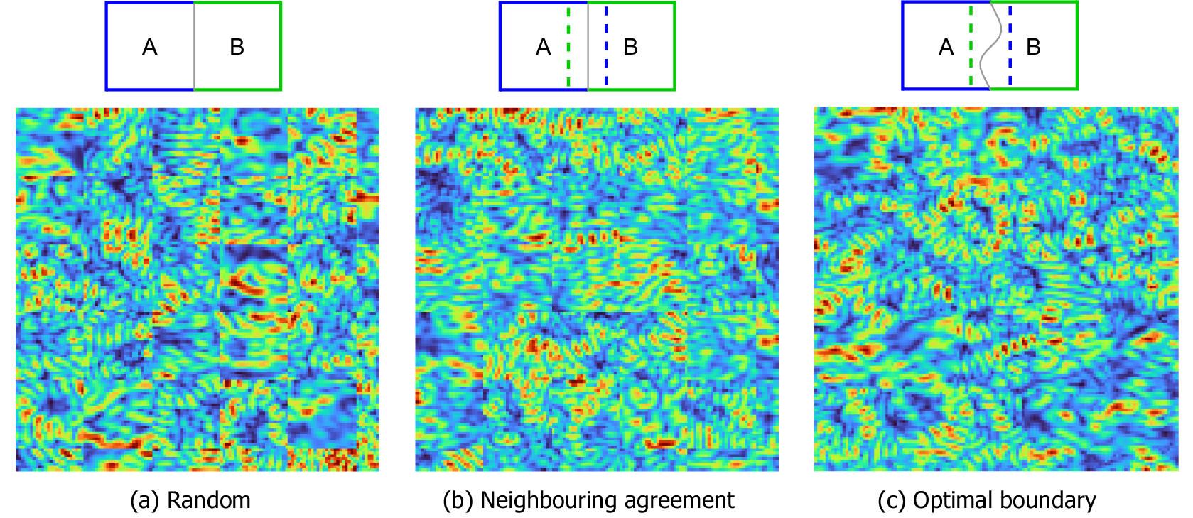
A naive approach to this, shown in Figure 7a, is to randomly join tiles together. However, this results in harsh structural disagreements along tile boundaries and large variations in local intensities between neighboring tiles, thus giving an unrealistic sampling of the noise distribution. To mitigate against these problems, we use an image quilting (Efros and Freeman, Reference Efros and Freeman2001) technique to stitch a random sampling of tiles together. For each stitching, a random subset of tiles is considered. The tile with the best neighboring agreement (Figure 7b) along the boundaries is selected for stitching. Finally, the minimal cost path is computed using the Dijkstra graph algorithm (Dijkstra, Reference Dijkstra1959) to find the optimal seam boundary between the two tiles (Figure 7c). We are, thus, able to generate a large dataset of ‘noise quilts’ of any size built from smaller synthesized noise tiles which can then be superposed onto naturally smooth numerical model target data (discussed in the following section). We generate noise quilts to match the size of training samples: $ 128\times 128 $
pixels (
$ 128\times 128 $
pixels ( $ {32}^{\circ}\times {32}^{\circ } $
), of which approximately 100,000 are generated. The method of applying noise quilts to clean targets will be detailed in Section 2.8 and the choice of region size will be justified in Section 3.2.
$ {32}^{\circ}\times {32}^{\circ } $
), of which approximately 100,000 are generated. The method of applying noise quilts to clean targets will be detailed in Section 2.8 and the choice of region size will be justified in Section 3.2.
Noise tiles generated by the DCGAN, joined using different patching methods.
2.7. Integrating prior knowledge on noise strength
Through visual analysis we observe that the geodetic noise patterns in the geostrophic currents occur on two scales. Small spatial scale noise appears as a consistent pattern distribution covering the full ocean field including over currents and other oceanographic features. Due to the small tile size of the training dataset, the noise generating networks in Section 2.5 are trained to focus on this small-scale noise distribution. However, it is observed that the noise also exhibits a deterministic pattern on a larger spatial scale, in which large patches of strong noise occur consistently across different geodetic products, that is, products produced using different geoid models. It is determined that such patches appear in areas associated with steep gradients in the geoid, and thus, occur along coastlines, around islands and along large seamounts. We exploit this knowledge of the deterministic large-scale noise patterns in order to make the training data more representative of the real-world geodetic data, with the aim of improving the modelling of the denoising filter.
The large-scale noise patterns are emulated in the training data using a noise strength map $ p $
which is produced by severely smoothing a geodetic MDT with a Gaussian filter. This process of filtering essentially smooths out the small-scale noise distribution and all gradients associated with oceanographic features. The remaining features are large smoothed patches which correlate with regions where noise is strong in the geodetic currents due to steep gradients in the geoid. Hence, this smoothed noise strength map
$ p $
which is produced by severely smoothing a geodetic MDT with a Gaussian filter. This process of filtering essentially smooths out the small-scale noise distribution and all gradients associated with oceanographic features. The remaining features are large smoothed patches which correlate with regions where noise is strong in the geodetic currents due to steep gradients in the geoid. Hence, this smoothed noise strength map $ p $
outlines the location and severity of the large scale deterministic noise pattern. It is then utilized to adjust the strength of the synthesized noise pattern learnt in Section 2.5, such that noise quilts are multiplied by
$ p $
outlines the location and severity of the large scale deterministic noise pattern. It is then utilized to adjust the strength of the synthesized noise pattern learnt in Section 2.5, such that noise quilts are multiplied by $ p $
before they are applied to the target.
$ p $
before they are applied to the target.
2.8. Method of applying noise model to clean targets
Noise quilts are applied to naturally smooth target data through addition in the first instance:
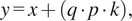 $$ y=x+\left(q\cdot p\cdot k\right), $$
where $ y $
is the noisy sample;
$ y $
is the noisy sample; $ x $
is the target;
$ x $
is the target; $ q $
is the noise quilt;
$ q $
is the noise quilt; $ p $
is the noise strength map produced from the prior geodetic geostrophic currents (discussed in Section 2.7); and
$ p $
is the noise strength map produced from the prior geodetic geostrophic currents (discussed in Section 2.7); and $ k $
$ k $ $ \in $
[0.5, 2.5] is a stochastic strength parameter, introduced to prevent over-fitting and improve generalization towards real-world data.
$ \in $
[0.5, 2.5] is a stochastic strength parameter, introduced to prevent over-fitting and improve generalization towards real-world data.
The resulting noisy sample is then re-scaled to better match the real noisy geodetic currents:
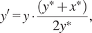 $$ {y}^{\prime }=y\cdot \frac{\left({y}^{\ast }+{x}^{\ast}\right)}{2{y}^{\ast }}, $$
where $ {y}^{\prime } $
is the re-scaled noisy sample;
$ {y}^{\prime } $
is the re-scaled noisy sample; $ {y}^{\ast } $
and
$ {y}^{\ast } $
and $ {x}^{\ast } $
represent the maximum values of the initial noisy sample (as in Equation 3) and the target, respectively. Therefore, the new maximum value of the re-scaled
$ {x}^{\ast } $
represent the maximum values of the initial noisy sample (as in Equation 3) and the target, respectively. Therefore, the new maximum value of the re-scaled $ {y}^{\prime } $
is set as the midpoint between maximum values
$ {y}^{\prime } $
is set as the midpoint between maximum values $ {y}^{\ast } $
and
$ {y}^{\ast } $
and $ {x}^{\ast } $
. Figure 8 shows the proposed noise application from Equation 4 for a cross-section of a random training sample. This strategy prevents exaggerated features in the noisy sample caused by adding the noise quilt in Equation 3, which would be undesirable as the denoising network would generally learn to dampen strong features during training in order to match the target, thus having a negative impact on performance to real data. We found empirically that higher velocity values were able to be retrieved when the denoising network was trained using this method of noise application in comparison to a simple additive approach.
$ {x}^{\ast } $
. Figure 8 shows the proposed noise application from Equation 4 for a cross-section of a random training sample. This strategy prevents exaggerated features in the noisy sample caused by adding the noise quilt in Equation 3, which would be undesirable as the denoising network would generally learn to dampen strong features during training in order to match the target, thus having a negative impact on performance to real data. We found empirically that higher velocity values were able to be retrieved when the denoising network was trained using this method of noise application in comparison to a simple additive approach.
The noise application method demonstrated for a cross section of a random training sample. The left plot shows cross-sections of the target (orange) against the target with added DCGAN noise (blue); the right plot shows cross-sections of the resulting noisy training sample where the sample has been re-scaled (blue) to more closely match the real currents, shown against both the target (orange) and a real sample of surface geostrophic currents computed from the DTU18_EIGEN-6C4 geodetic MDT (gray).
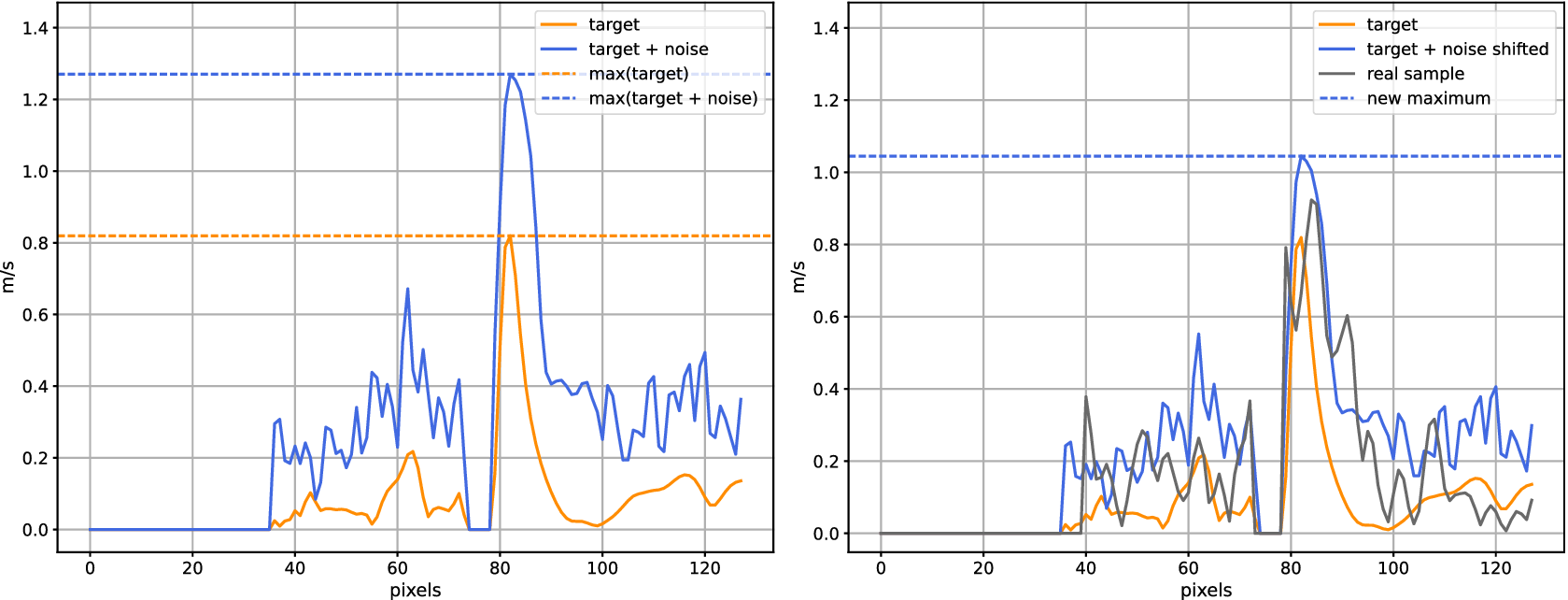
The proposed noise application, which integrates prior knowledge of the large-scale noise patterns and performs intensity scaling for a random training sample over the Gulf Stream region, is demonstrated in Figure 9. The resulting effect exhibits realistic noise behavior when compared against the real noisy data, particularly around the Greater Antilles.
A demonstration of the noise application showing (a) a target training sample from the HadGEM3-GC31-MM climate model; (b) a random noise quilt; (c) the associated noise strength map generated from the smoothed prior MDT; (d) the resulting synthetic sample in which the noise quilt has been applied to the target according to Equation 4 (with $ k $
=1.5); and (e) a real sample of surface geostrophic currents computed from the DTU18_EIGEN-6C4 geodetic MDT.
$ k $
=1.5); and (e) a real sample of surface geostrophic currents computed from the DTU18_EIGEN-6C4 geodetic MDT.
3. Denoising with Convolutional Autoencoders
3.1. The denoising network architecture
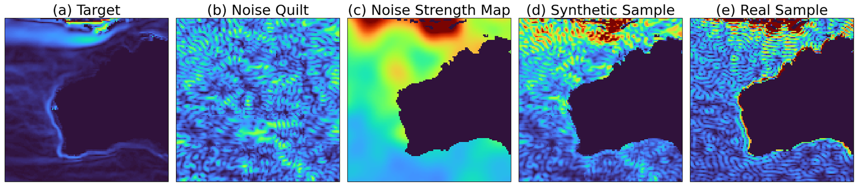
The denoising autoencoder network involves an encoder-decoder composition, where the encoder is passed a corrupted (noisy) input from which it learns a compressed representation stored as a latent vector (Schmidhuber, Reference Schmidhuber2015). The decoder then attempts to reconstruct the clean target as accurately as possible from the latent vector. Therefore, the network is guided to learn a denoising transformation, and thus learns to remove the type of noise present in the corrupted input. We incorporate convolutional layers into the autoencoder network, as they are known to improve performance for image denoising tasks, owing to a more powerful feature learning ability on spatial data (Zhang, Reference Zhang2018).
In this study, we use a denoising network consisting of four encoder and decoder blocks (Figure 10). Each encoder block consists of two 3x3 convolutional layers, each followed by a ReLU activation function and a 2x2 max pooling operation which downsizes each feature map by 2. At each max pooling layer, the number of feature channels is doubled. The feature dimensionalities for each convolutional block are detailed in Figure 10. The decoder is built inversely to the encoder, containing an up-sampling layer that doubles the feature maps and halves the number of feature channels each time. This is followed by two 3x3 convolutional layers, each followed by ReLU functions. Furthermore, we use batch normalization which has been found to boost denoising performance and speed of training (Zhang et al., Reference Zhang, Zuo, Chen, Meng and Zhang2017). Skip connections are utilized to preserve the fine spatial information that is lost during the down-sampling and up-sampling operations (Ronneberger et al., Reference Ronneberger, Fischer and Brox2015). These skip connections enable the passing of feature maps from earlier layers in the encoder to later layers in the decoder along the contracting path, and are joined via concatenation. Finally, a fully connected 1x1 convolutional layer is used and a 2D image is outputted.
The denoising autoencoder network architecture.
3.2. Training process
The CDAE network is trained on the constructed training dataset, discussed in Section 2, in which a synthesized noise model is applied to a naturally smooth dataset (via Equations 3 and 4) to construct noisy input and clean target pairs. Training images are chosen to be $ 128\times 128 $
pixels (
$ 128\times 128 $
pixels ( $ {32}^{\circ}\times {32}^{\circ } $
for a 1/4° map). We found that our denoising network performed best with inputs of this size, which may be due to such region size containing sufficient oceanographic information while limiting the distortion due to the equidistant cylindrical projection onto the 2D grid. Furthermore, regions above (below) a latitude of 64°N (64°S) are discarded prior to training to avoid the most extreme projection distortion that occurs at the poles. Generated from a set of 8 climate models (Table 1), the CDAE training dataset consists of 217,580 (
$ {32}^{\circ}\times {32}^{\circ } $
for a 1/4° map). We found that our denoising network performed best with inputs of this size, which may be due to such region size containing sufficient oceanographic information while limiting the distortion due to the equidistant cylindrical projection onto the 2D grid. Furthermore, regions above (below) a latitude of 64°N (64°S) are discarded prior to training to avoid the most extreme projection distortion that occurs at the poles. Generated from a set of 8 climate models (Table 1), the CDAE training dataset consists of 217,580 ( $ 128\times 128 $
) regions which overlap every 32 pixels (8°). The dataset’s properties are summarized in Table 4. During training, each time a synthetic region is loaded, a random noise quilt is selected and applied to the sample to create a clean and noisy training pair. Note that, since the number of quilts is less than the number of training regions, the same quilt may be used multiple times over an epoch. However, the combinations of synthetic samples and noise quilts are unique across each epoch.
$ 128\times 128 $
) regions which overlap every 32 pixels (8°). The dataset’s properties are summarized in Table 4. During training, each time a synthetic region is loaded, a random noise quilt is selected and applied to the sample to create a clean and noisy training pair. Note that, since the number of quilts is less than the number of training regions, the same quilt may be used multiple times over an epoch. However, the combinations of synthetic samples and noise quilts are unique across each epoch.
Details of the denoising network training data constructed from the eight climate models’ data (Table 1).
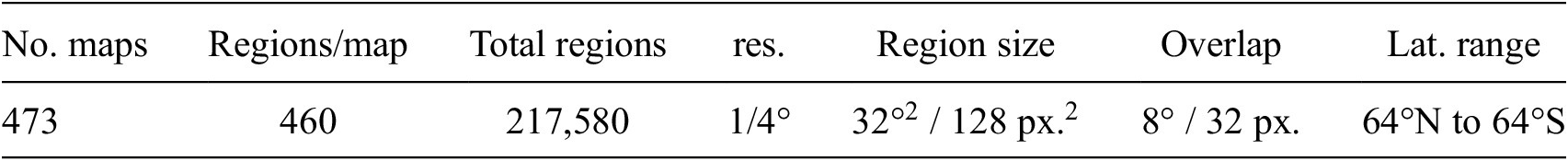
Note. In the table resolution and latitude are referred to as ‘Res.’ and ‘Lat.’ (resp.).
The CDAE network training process involves calculating the pixel-wise mean squared error (MSE) between output and target at each epoch,
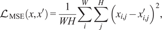 $$ {\mathrm{\mathcal{L}}}_{\mathrm{MSE}}\left(x,{x}^{\prime}\right)=\frac{1}{WH}\sum \limits_i^W\sum \limits_j^H{\left({x}_{i,j}-{x}_{i,j}^{\prime}\right)}^2, $$
where $ x $
is the target;
$ x $
is the target; $ {x}^{\prime } $
is the network output;
$ {x}^{\prime } $
is the network output; $ W $
and
$ W $
and $ H $
represent width and height of the images (resp.); and
$ H $
represent width and height of the images (resp.); and $ i,j $
denote a pixel’s row and column number. The computed error is then used to improve the network’s next prediction through back propagation using gradient descent. As the training images include regions over both ocean and land, land values are ignored during loss calculation to avoid irrelevant pixels negatively influencing back propagation. We use the Adam (Kingma and Ba, Reference Kingma and Ba2014) optimization algorithm and a learning rate of 0.001 with no decay schedule.
$ i,j $
denote a pixel’s row and column number. The computed error is then used to improve the network’s next prediction through back propagation using gradient descent. As the training images include regions over both ocean and land, land values are ignored during loss calculation to avoid irrelevant pixels negatively influencing back propagation. We use the Adam (Kingma and Ba, Reference Kingma and Ba2014) optimization algorithm and a learning rate of 0.001 with no decay schedule.
Data augmentation is implemented to avoid over-fitting, that is, when a network learns the specific characteristics of a training dataset too well. Data augmentation increases the variation seen by the network which involves synthesizing new data by introducing modifications of each training sample into the training dataset. This was achieved by randomly applying a set of geometric transformations to each training pair, including horizontal and vertical flips, and rotations by a multiple of 90°.
As discussed in Section 2.7, we observe that large-scale noise patterns occur in regions associated with steep geoid gradients. We, therefore, provide the denoising network with the associated geoid gradients of the loaded input region during training. This is done by passing the geoid gradients as a 2D image of the same size as the input through an extra channel via concatenation, both at training and testing time. This allows the network to learn the relationship between the noise strength and the steepness of geoid gradients. This has the effect of stimulating the network’s attention on these more sensitive regions, following a similar idea as in Derakhshani et al. (Reference Derakhshani, Masoudnia, Shaker, Mersa, Sadeghi, Rastegari and Araabi2019).
3.3. Ablation study on proposed components
We perform an ablation study of the different processes in creating the input data. We evaluate the respective contributions of the proposed processes in creating a quality dataset, both in turn and in combination. The first modification uses the noise strength map to introduce large scale noise variations to the synthetic noise quilts, detailed in Sections 2.7 and 2.8. The second modification involves passing the geoid gradients of the considered regions via an extra channel to the denoising network, detailed in Section 3.2. It is important to note that without the application of the noise strength map to the synthetic noise which emulates large-scale noise in the synthetic training data, the geoid gradients will not have any correlation with synthetic noise regions and the network would not implicitly be guided to learn the relationship between large-scale noise patches and steep geoid gradients. Thus, this second process cannot be evaluated in isolation and must always be combined with the first. The third process is random data augmentations, detailed in Section 3.2.
We train each configuration over 80 epochs, with batch size 512 and use 5-fold cross validation to determine the best epoch to be applied to the independent testing data. The process for this is as follows: five variations of the dataset are created where, for each version, a different fifth of the dataset is not used for training but instead used for validation. Then the network is trained from scratch over each five dataset variations and performance is measured on the unseen validation portion for every training epoch. The trained model from the epoch with the highest validation score is saved, obtaining five different ‘best performing’ models.
To make the ablation study unbiased to a particular data processing method, we require an independent testing dataset to validate results across all trained models. Therefore, to quantitatively assess how well noise is removed and oceanographic features are preserved, we create an ablation testing dataset of noisy input and target pairs. We obtain residual geodetic noise by removing the Gaussian filtered product from the noisy geodetic currents. We then apply this residual geodetic noise onto a subset of the climate model data, kept aside during training. The residual product is useful in this case as it contains realistic noise behavior such as large scale patches of strong noise which are known to occur. Measuring the effect of each modification towards removing this type of noise provides an independent way to estimate generalizability, that is, performance to unseen data. On the ablation test dataset, peak signal-to-noise ratio (PSNR) and structural similarity index (SSIM) scores are then calculated between the denoised outputs and the clean targets and averaged across the five folds (Wang et al., Reference Wang, Bovik, Sheikh and Simoncelli2004), shown in Table 5.
Ablation study of the different processes in creating the final training dataset for the denoising network: using the noise strength map; passing geoid gradients as an extra channel and applying data augmentations.
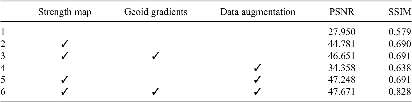
Note. Results presented are an average over the five folds from the best respective epoch of each model (obtained from the validation results) on the ablation test dataset.
The best result, with a PSNR of 47.671 and a SSIM of 0.828 (row 6), is achieved by the run that incorporates the noise strength map, passes the geoid gradients via an extra channel and applies data augmentations. The most effective modification is the use of the noise strength map, where any run using the strength map yields the biggest relative increase for PSNR (rows 2 and 5). This reinforces the notion that the more realistic the training data, the better a model can generalize to unseen data. Table 5 also shows that passing geoid gradients consistently improves denoising performance (rows 3 and 6), and shows the biggest increase for SSIM when combined with data augmentation (row 7). We use the best performing training data configuration (row 6) for all remaining experiments in this paper.
4. Results
In this section, using the best-performing configuration from Section 3.3, we train the CDAE network over 80 epochs, with a batch size of 512. We use 70% of the synthetic dataset for training, 20% for validation, and set aside 10% as unseen testing data. To facilitate this split, both synthetic clean regions and noise quilts are split to ensure that there is no crossover across datasets. First, we present the training and validation curves and secondly, we demonstrate the ability of the trained CDAE network to denoise unseen synthetic testing data. Thirdly, we assess the performance of the trained CDAE network when applied to real-world geodetic geostrophic currents. Here, a qualitative analysis of the denoised outputs is performed; results are then compared against the conventionally smoothed currents. We assess the performance of the network against the currents derived from the CNES-CLS18 MDT (Mulet et al., Reference Mulet, Rio, Etienne, Artana, Cancet, Dibarboure, Feng, Husson, Picot, Provost and Strub2021) using the root mean squared difference (RMSD), mean absolute difference (MAD) and a purpose-designed quantitative evaluation metric, which aims to quantify the two main components of denoising performance: the preservation of strong current velocities and the level of noise removal.
4.1. Denoising results on synthetic data
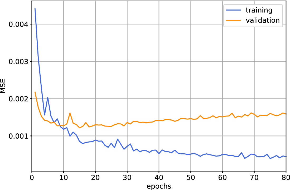
The training and validation curves show that the network learns quickly (Figure 11), where epoch 15 is found to score the lowest MSE. The validation curve then indicates gradual over-fitting as the training loss decreases while the validation loss increases. However, the validation loss remains relatively low across all epochs. Thus, we choose epoch 15 as the number of training epochs for our final network. The trained CDAE is applied to a set of synthetic testing samples, shown in Figure 12, across four major current systems that each play an important role in the global ocean circulation, but which vary in terms of complexity and signal (current strength) to noise ratio: the Gulf Stream (GS), the Kuroshio Current (KC), the Agulhas Current (AC) and the Brazil-Malvinas Confluence Zone (BMCZ). We present these outputs across multiple epochs, including the previously determined best validation epoch. It is observed that the CDAE filtering method is effective at removing the DCGAN generated synthesized noise. The positioning and shape of major current features across all regions in the filtered outputs closely match those in the target. It is evident that the CDAE network learns to accurately estimate the magnitude of the current velocities. This can be seen in the GS region for epochs greater than 1 (Figure 12: row 1), where the network accurately resolves the strong Gulf stream, the Loop Current (26°N, 86°W), as well as successfully disentangling noise from the relatively weak Caribbean current (18°N, 83°W), despite being of similar magnitude to the noise itself. Similarly, in the AC region (Figure 12: row 3), particularly at epoch 15, the network successfully removes noise without attenuating the powerful AC or the majority of the more intricate currents to the south. Although visual differences are subtle for epochs greater than 1, epoch 15 consistently retrieves the highest velocities at the core of each main current, thereby better matching the target. This reinforces the results computed on the validation dataset (Figure 11).
The training and validation curves from the CDAE network trained in Section 4.
A set of synthetic samples from the test dataset containing surface geostrophic current velocities (ms $ {}^{-1} $
) from the CMCC-CM2-HR4 climate model with DCGAN-produced noise quilts applied, denoised using the CDAE method across a range of CDAE training epochs showing the following regions: Gulf Stream (row 1), Kuroshio Current (row 2), Agulhas Current (row 3) and BMCZ (row 4).
$ {}^{-1} $
) from the CMCC-CM2-HR4 climate model with DCGAN-produced noise quilts applied, denoised using the CDAE method across a range of CDAE training epochs showing the following regions: Gulf Stream (row 1), Kuroshio Current (row 2), Agulhas Current (row 3) and BMCZ (row 4).
4.2. Application to real-world data
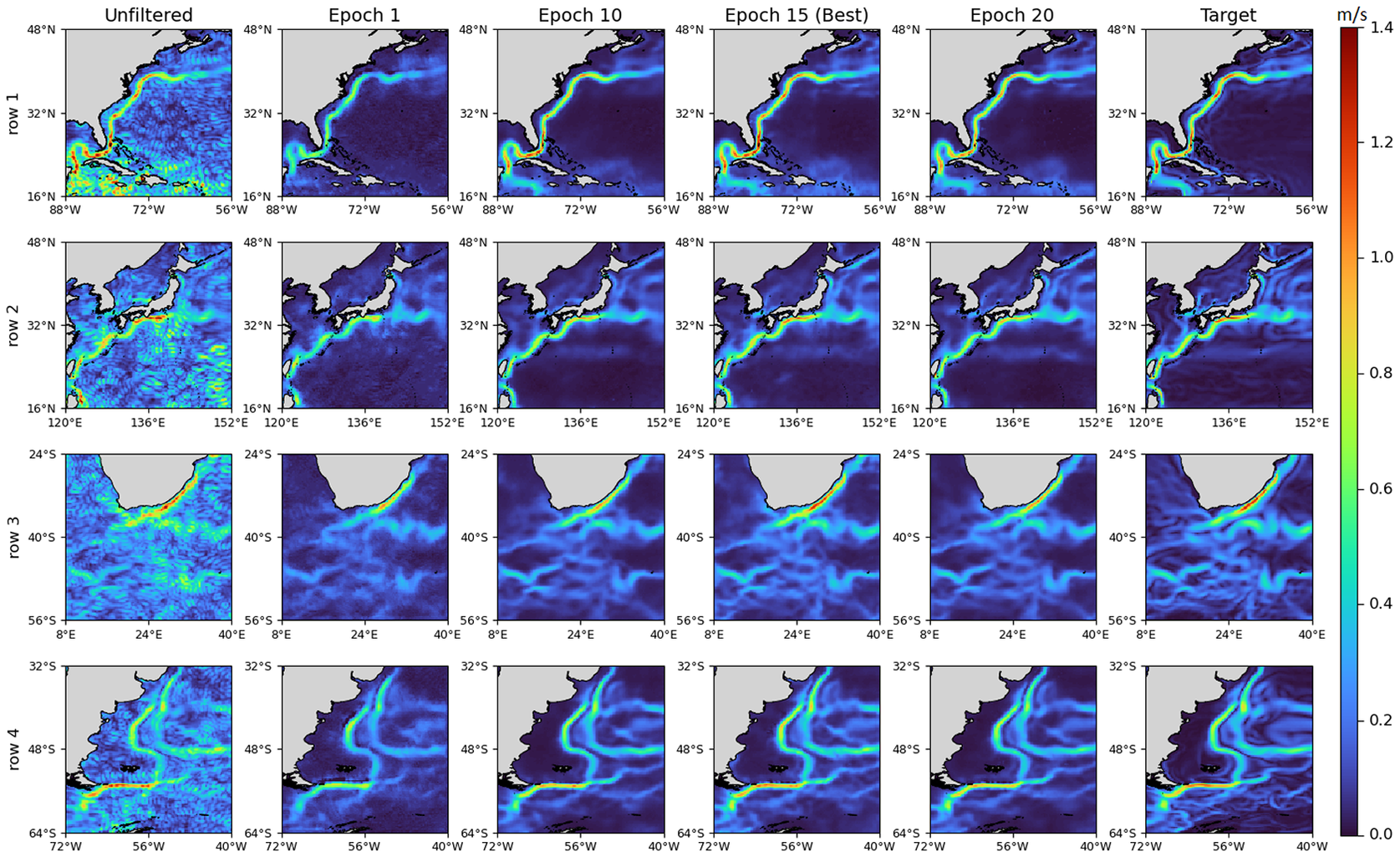
In this section, the trained CDAE network is applied to real-world geostrophic currents, computed from the DTU18_EIGEN-6C4 geodetic MDT. As for the synthetic case, it can be seen that the denoising method is effective by epoch 15 (Figure 13). In comparison to the unfiltered product, geodetic noise has been largely eliminated, while the major currents, and even weaker, finer-scale currents, are preserved or revealed with little attenuation. For the GS region (Figure 13: row 1), both the GS and the Loop Current in the Gulf of Mexico are well resolved, with the network at epoch 15 estimating higher velocities off the coast of the Yucatan peninsula and a clearer structure in the Gulf of Mexico, in comparison to other epochs. By epoch 15 in the KC region (Figure 13: row 2), the current structure is clear, although there is a small patch of very weak noise in the bottom left of the region; the only instance of this across the four regions. For the AC region (Figure 13: row 3), the network preserves the strength of the AC, while revealing finer details such as the meanders of the retroflection and the intricate current structures to the south, also seen in the synthetic data (although with some differences in details). Furthermore, for the BMCZ region (Figure 13: row 4), the confluence zone is more clearly resolved after the network has trained for 15 epochs. In particular, the zonal currents along the Sub-Antarctic front of the Antarctic Circumpolar Current are stronger and more detailed (48°S-58°S). Across all regions, there is little difference in the current estimates between epochs 15 and 20, indicating that the model has converged and stabilized by epoch 15. Finally, it is worth noting that the success of the CDAE in removing noise without attenuating the underlying currents, indirectly demonstrates the efficacy of using the DCGAN synthesized noise to create a training dataset.
Surface geostrophic current velocities, (ms $ {}^{-1} $
) computed from the DTU18-EIGEN-6C4 MDT, denoised using the CDAE method across a range of epochs showing the following regions: Gulf Stream (row 1), Kuroshio Current (row 2), Agulhas Current (row 3) and BMCZ (row 4).
$ {}^{-1} $
) computed from the DTU18-EIGEN-6C4 MDT, denoised using the CDAE method across a range of epochs showing the following regions: Gulf Stream (row 1), Kuroshio Current (row 2), Agulhas Current (row 3) and BMCZ (row 4).
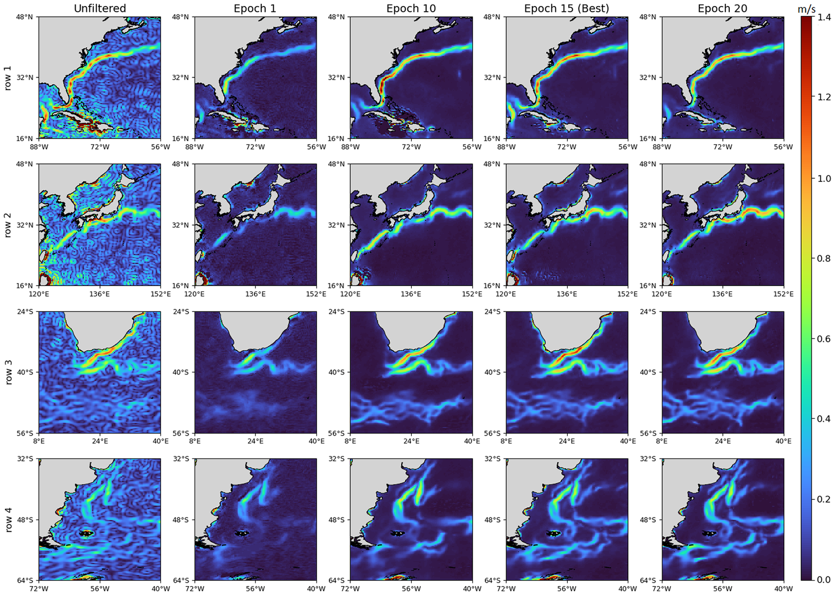
4.3. Comparison against Gaussian filtering
We compare the CDAE denoising method against a traditional isotropic filter, in which the surface geostrophic currents are computed from the Gaussian filtered geodetic MDT. This experiment is performed on the DTU18-EIGEN-6C4 MDT. The Gaussian filtered outputs (Figure 14) suffer from significant attenuation of high velocities as the filter radius increases. This is demonstrated clearly via the GS (Figure 14: row 1) and the KC (Figure 14: row 2) regions, which see a decrease of $ \sim $
0.3 ms
$ \sim $
0.3 ms $ {}^{-1} $
in maximum velocity values as the filter radius increases from 50 km to 70 km. While such important oceanographic features are lost, a significant level of noise remains in the open ocean of these regions. Conversely, the CDAE method yields high velocities while effectively removing the noise.
$ {}^{-1} $
in maximum velocity values as the filter radius increases from 50 km to 70 km. While such important oceanographic features are lost, a significant level of noise remains in the open ocean of these regions. Conversely, the CDAE method yields high velocities while effectively removing the noise.
Surface geostrophic current velocities (ms $ {}^{-1} $
) computed from the DTU18-EIGEN-6C4 MDT filtered using a Gaussian filter across a set of filter radii compared against the CDAE outputs at 15 epochs showing the following regions: Gulf Stream (row 1), Kuroshio Current (row 2), Agulhas Current (row 3) and BMCZ (row 4).
$ {}^{-1} $
) computed from the DTU18-EIGEN-6C4 MDT filtered using a Gaussian filter across a set of filter radii compared against the CDAE outputs at 15 epochs showing the following regions: Gulf Stream (row 1), Kuroshio Current (row 2), Agulhas Current (row 3) and BMCZ (row 4).

In addition to a loss of high velocities, the Gaussian smoother also suffers from imprecise positions of each current and finer-scale details are diminished across all regions. Areas near steep gradients appear to absorb this signal as the degree of smoothing increases. Moreover, not only is real signal absorbed by nearby areas, but the contaminative noise appears to be spread out rather than removed. This issue is illustrated well in the AC region (Figure 14: row 3), in which the relatively low and fine-scale velocities South of latitude 46°S are completely lost at filter radius 70 km. In contrast, the CDAE network retrieves significant detail at the same latitudes. In order to reach a reasonable level of noise removal using a traditional Gaussian smoother, the currents become severely attenuated, and thus there is an undesirable compromise in which important features are diminished or lost.
A significant benefit of the CDAE method over conventional smoothing is the ability to adaptively remove noise across a region. This is best illustrated via the GS region (Figure 14: row 1), specifically around the Greater Antilles (20°N, 76°W), in which noise is significantly reduced by the CDAE network, while high velocities and precise current positions are retrieved for the GS itself. In contrast, for the Gaussian filter, noise remains an issue in this area at both 50 km and 70 km filter radius despite significant smoothing.
4.4. Quantitative analysis
We compute the RMSD and MAD scores (Table 6) to quantitatively compare our method against the geostrophic currents derived from the Gaussian-filtered MDT for filter radii 50 km and 70 km, using the CNES-CLS18 MDT as a reference. These metrics measure the closeness (lower is better) of the denoised outputs versus a reference metric, where RMSD is more sensitive to outliers than MAD. For the GS and KC regions, the CDAE scores were significantly lower for both metrics. These two regions have similar characteristics in that they contain a very strong and fast current, with less medium current activity in the surrounding area, when compared to the other regions. This possibly demonstrates that a strength of the CDAE method is its ability to resolve strong velocities more accurately than traditional filters. For the BMCZ region, the RMSD of the CDAE output is approximately half those of the Gaussian filtered, while the MAD scores are roughly the same. A similar effect is observed on the AC region, though more exaggerated, where results show a higher MAD on the CDAE output than for the Gaussian filtered. This pattern indicates that the Gaussian filtered outputs contain a subset of predicted pixels with high error, which are exaggerated in the RMSD but smoothed over in the MAD. It is likely that the source of this high error is due to the Gaussian filter’s attenuation of the currents. When averaged over all regions, the CDAE gives lower RMSD and MAD scores than the Gaussian filter, by approximately 54% and 34% (resp.) Furthermore, to validate the heuristic of selecting the best epoch using the validation curve in Section 2.5, we repeated the RMSD and MAD computations across all epochs for both the CNES-CLS18 and the CNES-CLS22 (Schaeffer et al., Reference Schaeffer, Pujol, Veillard, Faugere, Dagneaux, Dibarboure and Picot2023) MDTs. Results showed that epoch 16 provided the lowest overall RMSD and MAD for both references, which agrees well with and reinforces the results found on the validation dataset (Section 2.5), where epoch 15 scored the best.
The root mean squared difference (RMSD) and mean absolute difference (MAD) between denoised DTU18-EIGEN-6C4 currents from Gaussian filtering (at filter radii 50 km and 70 km) and the CDAE method (at epoch 15) against the reference surface CNES-CLS18.
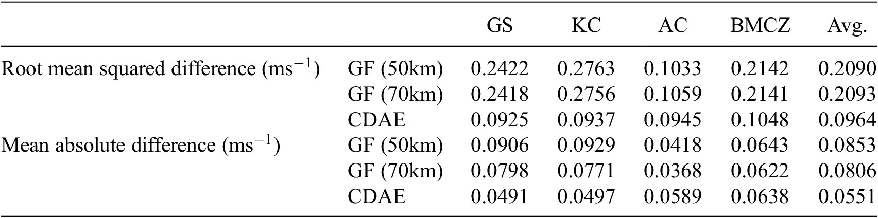
Note. Scores are shown over different geographical regions: the Gulf Stream (GS), the Kuroshio Current (KC), the Agulhas Current (AC) and the BMCZ. The final column shows the average of each row.
We design a quantitative evaluation metric which focuses on the main components of filtering performance: the preservation of current signal and the level of noise removal. First, an approximate mask outlining the position of each main current is obtained automatically from an MDT. The average velocity is then computed over this mask for each region which we denote as the ‘signal-preservation’ average. In order to reduce bias towards either filtering method, the recent CNES-CLS18 MDT is used to produce this mask. In practice, geostrophic currents computed from the CNES-CLS18 MDT are thresholded above 0.5 ms $ {}^{-1} $
to reveal the overall shape of the important currents. Secondly, a corresponding area (
$ {}^{-1} $
to reveal the overall shape of the important currents. Secondly, a corresponding area ( $ {5}^{\circ}\times {5}^{\circ } $
box) of low oceanographic activity near to the main current is manually identified for each region over which the average velocity is calculated. In practice, these regions are selected near main currents and in areas with consistently low velocities across all MDTs, that is, areas in which it can be assumed that the majority of the signal is due to geodetic noise. We denote this value as the ‘noise-removal’ average. Finally, the signal-preservation average is divided by the noise-removal average to obtain a ratio value for each region. Thus, the resulting ratio values indicate preservation of oceanographic signal versus level of noise removed, in which a higher value indicates better filtering performance. Signal-preservation, noise-removal and subsequent ratio values are shown in Table 7 across four geographical regions containing the main currents.
$ {5}^{\circ}\times {5}^{\circ } $
box) of low oceanographic activity near to the main current is manually identified for each region over which the average velocity is calculated. In practice, these regions are selected near main currents and in areas with consistently low velocities across all MDTs, that is, areas in which it can be assumed that the majority of the signal is due to geodetic noise. We denote this value as the ‘noise-removal’ average. Finally, the signal-preservation average is divided by the noise-removal average to obtain a ratio value for each region. Thus, the resulting ratio values indicate preservation of oceanographic signal versus level of noise removed, in which a higher value indicates better filtering performance. Signal-preservation, noise-removal and subsequent ratio values are shown in Table 7 across four geographical regions containing the main currents.
The signal-preservation, noise-removal and ratio values (signal-preservation divided by noise-removal) on the denoised DTU18-EIGEN-6C4 currents using a Gaussian filter (GF) at filter radii 50 km and 70 km and the CDAE method at epoch 15, and finally the CNES-CLS18 reference surface over different geographical regions.
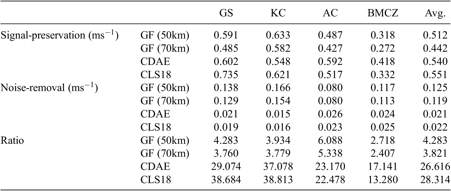
Note. The Gulf Stream (GS), the Kuroshio Current (KC), the Agulhas Current (AC) and the Brazil-Malvinas Confluence Zone (BMCZ). The final column shows the average of each row.
We note that the Gaussian filtered outputs follow an expected trend where signal-preservation and noise-removal are both higher for the 50 km filter radius, indicating lower attenuation but at the cost of more noise, which gives confidence in the technique used to compute this denoising metric. Furthermore, despite the fact that the Gaussian filtered currents at radius 50 km achieve a higher ratio than at 70 km, from visual inspection it can be seen that this product still contains significant noise (Figure 14); this further demonstrates the undesirable trade-off when using a Gaussian filter. Results show that both Gaussian filtering and the CDAE method provide similar signal-preservation values to the CNES-CLS18. However, only the CDAE method matches the noise-removal values of CNES-CLS18 in order of magnitude. Overall, ratio values achieved by the CDAE are much higher (better) than those of the Gaussian filtered at both filter radii, and are comparable in magnitude to those of the CNES-CLS18 (Table 7).
5. Concluding Discussion
In this paper, we have presented a deep-learning pipeline to remove the noise present in the geostrophic currents computed from a geodetic MDT. A generative network is trained to closely estimate the noise distribution of noisy geodetic data, and then to construct a novel training dataset of contaminated geodetic currents with corresponding noisy-free examples. In order to better represent the real geodetic data in the training data, several techniques have been adopted to prevent overly exaggerated features and to preserve global noise strength patterns. An ablation study on the different data processing methods proposed demonstrated that the use of prior knowledge benefits the network. This strategy of dataset creation is directly applicable to other blind image-denoising problems in the climate sciences in which the clean ground-truth does not exist but model data is available. Finally, a CDAE network is trained on the constructed training dataset and results are presented on real-world data.
Traditional isotropic spatial filtering causes attenuation along steep gradients in the MDT associated with currents of high interest during the noise removal process. It is shown qualitatively that the CDAE method significantly improves upon conventional Gaussian filtering in terms of reducing attenuation. Important oceanographic features are consistently preserved by the CDAE network and much higher velocities are retrieved while levels of noise are kept consistently low across all tested geographical regions. Quantitative analysis, using RMSD and MAD, confirmed these findings, showing that strong velocities are more accurately resolved using the CDAE method than Gaussian filtering and overall that the CDAE’s denoised currents more closely matched a reference MDT constructed from various data sources. A further quantitative evaluation method was designed to assess the level of attenuation of important features in conjunction with the level of noise removal in the case of blind-image denoising, which demonstrated the significant improvement achieved by the CDAE method compared to traditional Gaussian filtering.
An important benefit of the deep learning approach is the ability to exploit prior knowledge of the geodetic noise patterns. In turn, this allows the CDAE network to adaptively remove noise within a given region, such that the severe noise that occurs near the coast and around islands (coinciding with steep gradients in the geoid) is significantly reduced without bleeding into nearby areas. A further benefit of the CDAE denoising method is that it can be trained to remove different types of noise depending on the training dataset given. This allows our method to be adapted to different types of problems. This could involve refining the method to denoise the geostrophic currents associated with the satellite-only geoid which contains significantly more noise than the high-resolution geoid used in this study (produced using a combination of data sources including both satellite and ground data.) A current limitation of the proposed method is that the trained network denoises relatively local regions of the global MDT. This could be addressed in future work, where the method could be adapted to denoise larger regions or even the full global map.
Looking to the future, improvements in gravity field determination from geodetic missions such as ESA/NASA’s approved MAGIC (Mass-Change and Geosciences International Constellation) mission should reduce the level of noise in geodetic MDT and associated ocean current estimates (Massotti et al., Reference Massotti, Siemes, March, Haagmans and Silvestrin2021). However, they are unlikely to eliminate it completely as there will still be a mismatch in scales between the geoid and the MSS. Therefore, filtering methods, such as the one developed in this paper, will still be necessary for the foreseeable future. Similarly, it will still be necessary to optimally filter geodetic currents to provide the best possible longer-wavelength complement to finer-scale currents measured directly by new missions such as ESA’s Harmony mission (López-Dekker et al., Reference López-Dekker, Biggs, Chapron, Hooper, Kääb, Masina, Mouginot, Nardelli, Pasquero, Prats-Iraola, Rampal, Stroeve and Rommen2021). Indeed, deep learning methods offer an opportunity to optimally combine current observations from a range of sources taking into account the error characteristics of each source.
Acknowledgments
The authors would like to thank Felix Richards for the helpful discussions. This work was carried out using the computational facilities of the Advanced Computing Research Centre, University of Bristol - http://www.bris.ac.uk/acrc/. Additionally, we acknowledge the World Climate Research Programme, which provided the CMIP5 and CMIP6 data.
Author contribution
Conceptualization: all authors; Data curation: L.G. and R.J.B; Data visualization: L.G.; Methodology: all authors; Software development: L.G.; Supervision: R.J.B. and A.P.; Writing original draft: L.G.; Writing—reviewing and editing: all authors. All authors approved the final submitted draft.
Competing interest
The authors declare none.
Data availability statement
All data used in this study are publicly available and detailed above. Code and trained weights are available at https://github.com/laura-gibbs/CDAE_pipeline.
Ethics statement
The research meets all ethical guidelines, including adherence to the legal requirements of the study country.
Funding statement
L.G. was supported by the Natural Environment Research Council (NERC) grant NE/R011621/1.


 Open access