1. Introduction
European pension funds and insurers managed more than a combined €18.5 trillion worth of assets in 2020.Footnote 1 For these institutions it is crucially important to attain precise estimates of long-term discount rates for their asset management and for regulatory liability valuation. Despite its practical importance and potential welfare consequences, modeling and examining the very long end of the nominal term structure has attracted limited attention in academic research thus far.
This paper aims to fill this gap in the literature by studying a yield curve extrapolation technique that produces discount rates suitable for regulatory valuation. This technique is not only easy to implement due to its few estimable parameters, but it also relies on prices of bonds traded on the market.
We build our method, the Modified Nelson-Siegel (MNS) curve, on the work of Nelson and Siegel (Reference Nelson and Siegel1987), in three consecutive steps: (i) we perform the standard Nelson-Siegel (NS) estimation, then (ii) using the resulting parameters, we calculate the convexity correction that is based on a VAR(1) of these parameters, then (iii) we re-estimate the NS parameters after correcting for the convexity effect. This method gives us the MNS curve. A distinct feature of this yield curve is that is accounts for the impact of convexity along the maturity spectrum, and thereby offers estimates that are consistent with arbitrage-free affine term-structure models, as shown by Christensen et al. (Reference Christensen, Diebold and Rudebusch2011) and Christensen et al. (Reference Christensen, Diebold and Rudebusch2009).
We assess the goodness of fit of these regulatory curve candidates by constructing a pair of measures similar to that of the ‘noise measure’ of Hu, Pan, and Wang (Reference Hu, Pan and Wang2013). We fit a smooth curve to bonds with less than 20 years to maturity to determine the theoretical curve, which then we extrapolate for longer maturities.Footnote 2 We repeat this exercise for both the standard NS and the MNS methods. Next, we construct two price distortion (PD) measures that allow us to compare the model's fit in both the intermediate (in-sample) and long (out-of-sample) maturity segments separately. Comparing the two methods, we find that the average PD is 6.42 bps and 5.72 bps for the standard NS and the MNS model, respectively. The MNS approach, which is theoretically superior to the NS approach since it excludes arbitrage opportunities, produces the smallest and least dispersed PD measure in sample with a range of 2.00–13.44 bps over time, reflecting its superior in-sample-fit. Shifting our focus to the long end of the curve, we find that, while the average NS-implied PD is 18.82 bps, adjusting for convexity significantly increases the PD: the MNS measure has a PD of 42.97 bps on average with a range of about 50 bps. While these numbers are non-negligible, relative to the magnitude of yields of ultra-long maturities, they suggest that our simple model does a reasonable job at predicting long maturity bond yields.
Next, we examine the average fitting error of long maturity bonds, which we call the bias. The size of this measure depends on the method: the bias derived from the standard NS approach is moderately large, on average about −1.54 bps with a time-series range of 100 bps, and with the bias switching signs throughout the sample. In contrast, the MNS method shows that the bias is persistently negative, on average −38.80 bps, with a smaller range of 55 bps. A negative bias is a product of observed yields being consistently lower than those implied by our pricing model. We postulate that this could be due to two factors: while we cannot exclude the possibility of some model (fitting) error, economic factors that could lead to structural distortions in the different maturity segments can also cause these errors. In case of the latter, market segmentation stemming from demand pressures on certain yield segments, differential risk exposures or liquidity premiums could drive a wedge between the model-implied yields and the ones observed on the market.
We derive these regulatory curve candidates from German data and study the period between January 2000 and March 2015. The German nominal bond market not only serves as the benchmark Eurozone sovereign bond market, but arguably, it is the closest to being free of default risk in our sample period.Footnote 3 Overall, in Germany, due to its large and liquid bond market, the segmentation and liquidity driven components of fitting errors are likely to be small, since market liquidity facilitates arbitrage and thereby keeps asset prices close to fundamentals. In fact, this market is relevant from the regulatory perspective, since it is a key market to establish a risk-free term structure that is not affected much by default or liquidity effects.Footnote 4
Lastly, we present a pension case study that aims to shed light on the ongoing policy debate about the Ultimate Forward Rate (UFR) methodology and the use of swap rates for liability valuation. Motivated by the result of Christensen et al. (Reference Christensen, Lopez and Mussche2021) that NS curves can produce reliable long-term yield estimates, we model and extrapolate (very) long-term discount rates that are suitable for liability valuation of pension funds or insurers (P&Is). We find that our simple yield curve model based on the MNS approach produces reasonably small fitting errors both in-, and out-of-sample and would lead to prudentially stricter, that is lower, discount rates than those currently used. In practice, our results suggest that one could consider to base the extrapolation of very long term discount rates on the prices of these traded sovereign bonds, as opposed to interest rate swaps. In addition, our MNS method could be consistently implemented with the Smith-Wilson technique connecting traded asset maturities to the UFR, as described in Jørgensen (Reference Jørgensen2018) in more detail.
This paper contributes to three distinct strands of the literature: (i) to the discussion on long-term discount rates, (ii) the debate on the impact of regulation on the yield curve, as well as to (iii) the literature studying the causes of bond market segmentation.
First, we contribute to the discussion on long-term discount rates. The majority of papers in this literature segment derive long and ultra-long term discount rates using the interest swap curve and link its pricing dynamics to clientele demand of P&Is (Domanski et al., Reference Domanski, Shin and Sushko2017; Quaedvlieg and Schotman, Reference Quaedvlieg and Schotman2020; Balter et al., Reference Balter, Pelsser and Schotman2021). One caveat of this asset choice is that swaps are bilaterally negotiated contracts and thereby carry counterparty risk (Jarrow and Yu, Reference Jarrow and Yu2001; Duffie and Canabarro, Reference Duffie, Canabarro and Tilman2003), which could distort the resulting discount rates by a swap or counterparty risk premium. As an alternative, Christensen et al. (Reference Christensen, Lopez and Mussche2021) use a simple term structure model fitted on US Treasury securities, and show that extrapolating long-maturity bond yields by the Dynamic NS method produces discount rates that are comparable to predictions of professional forecasters. Similarly to J. H. E. Christensen, Lopez, and Mussche (ibid.), we choose to work with sovereign bonds, which are (near) default risk free and therefore produce discount rates that might be conceptually better suited for regulatory liability valuation. Of course, we cannot rule out that using bond yields for regulatory purposes might affect the pricing of these bonds.
Our work also relates to the discussion on the impact of regulation on the yield curve, more specifically price effects of the demand pressure arising from regulatory mandates. For instance, by using macroeconomic aggregates, Greenwood and Vissing-Jorgensen (Reference Greenwood and Vissing-Jorgensen2018) study the effect of P&Is on the 10 to 30-year segment of the yield curve. Using a cross-country sample, they find that in countries with large P&I sectors the spread is smaller, indicating that the preferred habitat demand of these institutions suppresses yields of long maturity bonds. Jansen (Reference Jansen2021) comes to a similar conclusion by studying the portfolio holdings of Dutch P&Is, and the impact of the introduction of UFR in the Solvency II framework in a panel of 20 European countries with a large insurance sector. Empirical evidence suggests that this regulatory demand pressure not only suppresses government bond yields, but as Klinger and Sundaresan (Reference Klinger and Sundaresan2019) show, also long maturity interest swap rates in the US, Europe and Japan.
And lastly, we contribute to the diverse literature on market segmentation. Market segmentation could arise when some investors do not have access to the overall yield curve due to regulatory constraints or their endogenously chosen investment horizon. Vayanos and Vila (Reference Vayanos and Vila2021) show that bond demand might be driven by preferred habitat investors, in which case demand shocks affect the cross-section of bonds differently. Greenwood and Vayanos (Reference Greenwood and Vayanos2010) provide empirical evidence for this demand shock following the 2004 UK pension reform.Footnote 5
Central banks' large scale asset purchases (and later the quantitative easing) can also result in local demand pressure (see Krishnamurthy and Vissing-Jorgensen, Reference Krishnamurthy and Vissing-Jorgensen2011; D'Amico et al., Reference D'Amico, English, López‐Salido and Nelson2012; D'Amico and King, Reference D'Amico and King2013; Christensen and Gillan, Reference Christensen and Gillan2022, among others). Alternatively, if local demand shocks are accompanied by limited arbitrage capital, pricing inefficiencies cannot be eliminated and become persistent along the yield curve (Shleifer and Vishny, Reference Shleifer and Vishny1997; Gromb and Vayanos, Reference Gromb and Vayanos2002; Liu et al., Reference Liu, Longstaff and Mandell2006; Ashcraft et al., Reference Ashcraft, Gârleanu and Pedersen2010; Gorton and Metrick, Reference Gorton and Metrick2010). Additionally, this arbitrage capital might move too slowly: either due to capital constraints (Mitchell et al., Reference Mitchell, Pedersen and Pulvino2007), agency problems of delegated asset management Duffie (Reference Duffie2010), or the regulatory cost of trading (Boyarchenko et al., Reference Boyarchenko, Eisenbach, Gupta, Shachar and Van Tassel2018). The noise measure of Hu et al. (Reference Hu, Pan and Wang2013) or its European counterpart of Malkhozov et al. (Reference Malkhozov, Mueller, Vedolin and Venter2017) aim to proxy for general funding conditions or slow-moving capital and are, to some extent, comparable to our PD measures.
Another driver of segmentation could stem from intermediate and long maturity bonds being exposed to risk factors to a different extent. The emergence of different levels of risk premiums affect the relative pricing along the yield curve. These alternate levels of risk premiums between intermediate and long-term yields can stem from the various sources: flight-to-safety flows (Longstaff, Reference Longstaff2004; Beber et al., Reference Beber, Brandt and Kavajecz2009; Ejsing and Lemke, Reference Ejsing and Lemke2011; Næs et al., Reference Næs, Skjeltorp and Ødegaard2011; Baele et al., Reference Baele L and Inghelbrecht K2020), credit risk and/or partial default or breakup risk (Simon, Reference Simon2015; De Santis, Reference De Santis2019), or liquidity differences either due to seasonedness (Krishnamurthy, Reference Krishnamurthy2002; Gürkaynak et al., Reference Gürkaynak, Sack and Wright2007; Bühler and Vonhoff, Reference Bühler and Vonhoff2011; Fontaine and Garcia, Reference Fontaine and Garcia2012; Kempf et al., Reference Kempf, Korn and Uhrig-Homburg2012; Schuster and Uhrig-Homburg, Reference Schuster and Uhrig-Homburg2012); or the sovereign-agency bond spreads (Longstaff, Reference Longstaff2004; Krishnamurthy and Vissing-Jorgensen, Reference Krishnamurthy and Vissing-Jorgensen2011; Schuster and Uhrig-Homburg, Reference Schuster and Uhrig-Homburg2012; Schwarz, Reference Schwarz2018). Unreported regressions indicate that the PD and bias measures are correlated with clientele demand proxies, and liquidity and other risk premiums that differ along the yield curve. As such, our estimates for these effects estimated from a large, liquid, and (near) default risk-free government bond market can serve as a benchmark for future studies on market segmentation.
The remainder of the paper is organized as follows. Section 2 presents the data and the methodology of the paper, while Section 3 presents the PD and bias measures for the various curve fitting methods. Section 4 discusses policy implications and presents a case study for liability valuation. Finally, Section 5 concludes.
2. Data and curve fitting methodology
2.1 The data
The data for our analysis come from Bloomberg. To fit the yield curve, we collect daily closing mid-quotes of German capital market securities and cross-sectional bond characteristics. For the pension case study in Section 4.2, the ultimate forward rate curve is provided to us by the Dutch National Bank (DNB).
To propose a simple and easy to replicate method for long-term yield extrapolation, we use a panel of daily bond prices (yields) from January 2000 through March 2015 of all German sovereign nominal capital market securities.Footnote 6 We focus our analysis on plain vanilla bonds with fixed maturities and coupons, and the same market conventions and microstructure. These bonds can be assigned to one of the four tenors: 2-year notes (Schaetze), 5-year notes (Bobls), and 10, or 30-year Bunds. Similar to other studies, we drop bonds with less than 6 months to maturity due to liquidity problems, however, in contrast to others in the literature, we do not impose an upper bound on remaining time to maturity.
In the resulting sample we have, on average, a cross-section of 52 bonds, with 6 bonds with maturities longer than 20 years. However, the cross-section varies over time, ranging between 38 and 56 issues of capital market securities, and 1 to 8 long maturity bonds at a time. The average maturity of bonds is 7.37 years. The average coupon is 4.14%, with a standard deviation of 1.72%, and the maturity dates of the bonds range from August 2000 to August 2046.
2.2 Constructing the yield curve
2.2.1 The Nelson-Siegel curve
Our aim in this paper is to offer a simple method to extrapolate long-term yields for liability valuation. The starting point is the Nelson-Siegel (NS) model (Nelson and Siegel, Reference Nelson and Siegel1987), some version of which Christensen et al. (Reference Christensen, Lopez and Mussche2021) show to produce reasonable discount rates, fit for regulatory valuation. This model not only provides a smooth, flexible parametric function, but as De Pooter (Reference De Pooter2007) describes, is capable of capturing many of the typically observed shapes of the term structure.
The NS curve assumes the following functional form for the zero-coupon yield curve, s:
where T − t denotes time to maturity and b = (β 0, β 1, β 2, τ) are model parameters to be estimated.
The parameterized zero-coupon yield curve of equation (1) is then used to price any coupon-bearing bond. Consequently, we can use market prices of bonds to back out the parameters in b. In particular, on each day of our sample, we estimate the model from observable market prices of bonds with remaining maturities between 6 months and 20 years. This results in a vector of parameters on each day, based on which we can predict the theoretical values of the observed bonds. In order to fit the model, we choose parameters b t by minimizing the duration-weighted sum of squared deviations between the observable and the model implied prices:Footnote 7

where N t is the number of bonds for a given day, P t are the prices observable on the market, whereas P i(b) is the model-implied price for coupon-paying bond i given the model parameters b, while D i,t is the Macaulay's duration for bond i.
In fact, one deviation from the approach of Hu et al. (Reference Hu, Pan and Wang2013) is that we do not estimate all parameters freely, but keep τ fixed for the analysis. In preliminary unrestricted estimations, τ proves to be badly identified with extreme values on days when the yield curve is flat. This suggests multicollinearity of the parameters, which we circumvent by fixing the parameter τ at its the median value obtained from the unrestricted estimation of the model. Keeping τ fixed, we re-estimate the rest of the parameters to obtain the fitted curves for each day in our sample.Footnote 8
Note that Hu, Pan, and Wang (ibid.) use the specification of Svensson (Reference Svensson1995) to describe the term structure. This specification has more parameters. Estimating models with a large number of parameters is nontrivial and brings the risk of overfitting. For example, even in the Nelson-Siegel model the τ parameter is hard to estimate on a day-to-day basis. Given that our goal is to extrapolate long-term interest rates, such overfitting is a major concern, which is why we choose the simpler Nelson-Siegel approach.
2.2.2 Convexity correction
A major theoretical drawback of the NS approach is that it does not generate bond prices that are theoretically arbitrage-free. To overcome this issue, Christensen et al. (Reference Christensen, Diebold and Rudebusch2011) and Christensen et al. (Reference Christensen, Diebold and Rudebusch2009) propose a correction to account for the main cause of this effect: convexity. They also show that adjusting for this effect, one can obtain a ‘modified’ NS model that is consistent with an arbitrage-free affine term structure model, like the Arbitrage-Free Generalized NS model of Christensen et al. (Reference Christensen, Diebold and Rudebusch2011). Appendix B provides the detailed steps to calculate the convexity correction.
Table 1 reports the descriptive statistics of the convexity correction along the different maturity segments of the yield curve. The average correction is 13.36 bps. Focusing on longer term bonds shows that convexity steeply increases with maturity. For long bonds, those with above 20 years of remaining time to maturity, the average effect is 82.10 bps, while for 25 + year bonds, this effect is on average 97.03 bps. These large values underline the importance of controlling for convexity in extrapolating long-term yields, and that it matters which model is used and how it is estimated.
Table 1. Summary statistics of the convexity correction

The table presents descriptive statistics of the convexity correction, abbreviated as CC below. It is following the definition of Christensen et al. (Reference Christensen, Diebold and Rudebusch2011) and Christensen et al. (Reference Christensen, Diebold and Rudebusch2009) and is calculated based on equations (B.3) and (B.4). The correction term is displayed for different maturity segments of the yield curve: intermediate maturities span 6 month to 20 years, long maturities above 20 years, while for ultra-long maturities bonds with more than 25 years of remaining maturity are considered. All measures are expressed in basis points. The sample spans January 2000 to March 2015, and the data come from Bloomberg.
2.2.3 The modified Nelson-Siegel curve
In this section we introduce the Modified NS (MNS) model to offer a simple and easily implementable method for extrapolating long-term yields for liability valuation. This method results in yield estimates that are consistent with the Arbitrage-Free Generalized NS approach of J. Christensen, F. Diebold, and G. Rudebusch (ibid.), although its implementation is simpler and therefore more accessible to practitioners, like P&Is.
Our proposed MNS curve is based on an iterative approach. First, we implement the NS model through the parameterized zero-coupon curve of equation (1), using market prices of bonds with remaining maturities between 6 months and 20 years. Next, we calculate the convexity correction from equation (B.3) for each bond and day in our sample.Footnote 9 We define the Convexity-Adjusted NS (CA-NS) yields as the difference between the yields predicted by the initial NS model and the convexity correction. This convexity correction is then used to re-estimate the NS parameters, b, each day, applying the same optimization process as in Section 2.2.1, where where we thus incorporate the convexity correction estimated in the first stage. As with the initial NS estimation, the preliminary unrestricted estimation results in a badly identified τ parameter, so we fix it at its median value obtained from the initial, unrestricted estimation of the model. Finally, keeping τ fixed, we repeat the estimation of equation (2) for the rest of the parameters in b for each day of the sample, using the convexity adjusted yields.
In the next section we introduce measures that allow us to formally quantify the goodness of fit, while we also offer plausible economic explanations for the reported ‘fitting errors’.
3. Empirical results
In this section, we focus on the goodness of fit of our proposed long-term extrapolation method. In short, we will demonstrate that (i) the fitting errors are not very large, especially relative to the size of the convexity correction shown in Section 2.2.2, therefore the MNS method seems also capable of producing reliable long-term discount rates; while (ii) we will also provide plausible economic explanations for any difference between model-implied and observed yields arising along the yield curve. To do so, we present two measures: the maturity-dependent PD measure and the bias.
We present these measures comparing three cases: (i) the standard NS estimation, (ii) a case where we subtract the convexity correction from the yields generated by the standard NS estimation, henceforth called CA-NS approach, and (iii) the case where we re-estimate the NS parameters after correcting for the convexity effect, that is the MNS model.
3.1 Measures of price distortion
To construct the PD measure, we follow Hu et al. (Reference Hu, Pan and Wang2013), henceforth HPW. For each day in the sample, given the set of parameters b t from one of the curve fitting methods, we calculate the difference between the fitted and observable market yields. HPW define noise as the dispersion of yields around the (entire) fitted yield curve, measured as the root mean squared pricing error. Our approach differs in that we separate pricing errors along the yield curve, resulting in two distinct sets of PD measures: one for intermediate, and another form long-term bonds.Footnote 10
For each date t, let b t be a vector of parameters with τ fixed at its unconditional median value: τ = 2.59 for the NS (and CA-NS) estimation, while τ = 1.85 for the MNS approach. On the given date t, there are N int.,t bonds in our sample with maturities between 6 month and 20 years and N long,t bonds with remaining maturities exceeding 20 years. Then for each of these bonds part of N int.,t andN long,t, we calculate the difference between $y_t^i$![]() and y i(b t), the observed market and the model-implied yields, respectively. To be precise, for each coupon-paying bond in our sample, we calculate the bond price that is implied by the model, and then calculate the yield-to-maturity y i(b t) for this model-implied bond price, and compare this to the observed yield $y_t^i$
and y i(b t), the observed market and the model-implied yields, respectively. To be precise, for each coupon-paying bond in our sample, we calculate the bond price that is implied by the model, and then calculate the yield-to-maturity y i(b t) for this model-implied bond price, and compare this to the observed yield $y_t^i$![]() . Then we define the PD measure as the dispersion around the fitted curve, that is the root mean squared pricing error of the given maturity segment of the yield curve separately:
. Then we define the PD measure as the dispersion around the fitted curve, that is the root mean squared pricing error of the given maturity segment of the yield curve separately:

where segment = [intermediate, long].
Although we fit the yield curve to bonds with maturities between 6 months to 20 years, the long maturity PD measure is based on a wider range of maturities. This is why the long maturity PD measure also serves as an ‘out-of-sample’ test for the fit of the yield curve. In choosing the 20-year maturity as our break-point, we are motivated by the European UFR discussion of Solvency II. The UFR is an extrapolation technique used to calculate long term discount rates for regulatory liability valuation of maturities that lie beyond the last liquid point. This point for euro-denominated interest rates is set at 20 years to maturity. More detailed discussion on these policy questions can be found in Section 4.
Table 2 presents the summary statistics of the PD measure for the various curve fitting approaches and for the period between January 2000 and March 2015. Panels A, B, and C present the PD and US noise measures provided by Jun Pan, respectively.Footnote 11 In Panel A, we compare the intermediate-maturity PD across the three methods. The average PD for the NS model is 6.42 bps, and 12.80 and 5.72 bps for the CA-NS, and MNS models, respectively. It appears that already for bonds with up to 20 years to maturity, adjusting for convexity makes a difference. The MNS approach produces the smallest and least dispersed PD measure (with a time-series range of 2.00 to 13.44 bps), followed by the standard NS model (2.80–23.84), and its convexity-adjusted implementation (2.88–28.36 bps). The crudeness of the simple adjustment for convexity is even clearer in Panel B. On the long end of the curve we observe that, while the average NS-implied PD is 18.82 bps, adjusting for convexity significantly increases the PD of long-term bonds: the MNS measure is 42.97 bps on average with a range of about 50 bps, while the CA-NS measure averages at 81.89 bps and peaks at 138.21 bps.
Table 2. Summary statistics of the PD measures and the bias
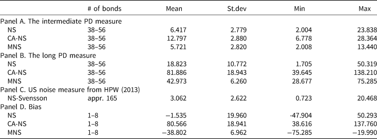
Figure 1, plotting the PD measures across the three fitting methods, confirms these observations. Figure 2, on the other hand, focuses on the PD measures derived from the smooth MNS curve along the maturity spectrum. The time series dynamics of the MNS PD measures are in line with the statistics of Table 2. The figure shows that the magnitude of the PD measures, especially that of the longer maturity segment, varies greatly over time, with large peaks around the financial and euro crises. Long yields have a somewhat poorer fit during this period, and thus their respective PD measure is persistently high(er).
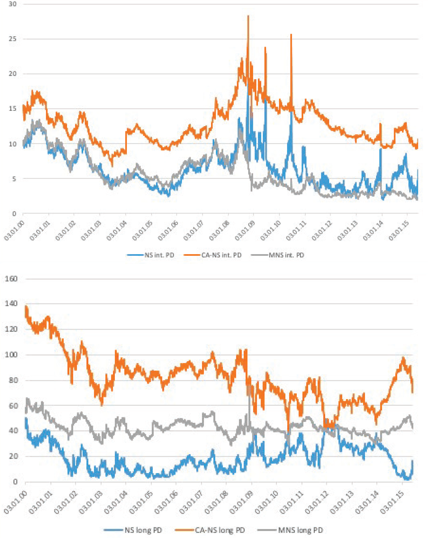
Figure 1. PD estimates across fitting methods. The figure plots the daily time series of the PD measures across the different curve fitting methods. The top panel shows the PD of intermediate-term bonds, while the bottom panel focuses on long-maturities (20+ years). PD is defined as the root mean squared deviation from the smooth curve fitted on German sovereign notes and bonds with maturities between 6 months and 20 years. For bonds with longer maturities, PD is based on the extrapolation of this smooth curve. The smooth curves are derived from the following methods: standards NS (blue), the CA-NS (orange), and the MNS (grey) approach. All measures are expressed in basis points. The sample spans January 2000 to March 2015, and the data come from Bloomberg.
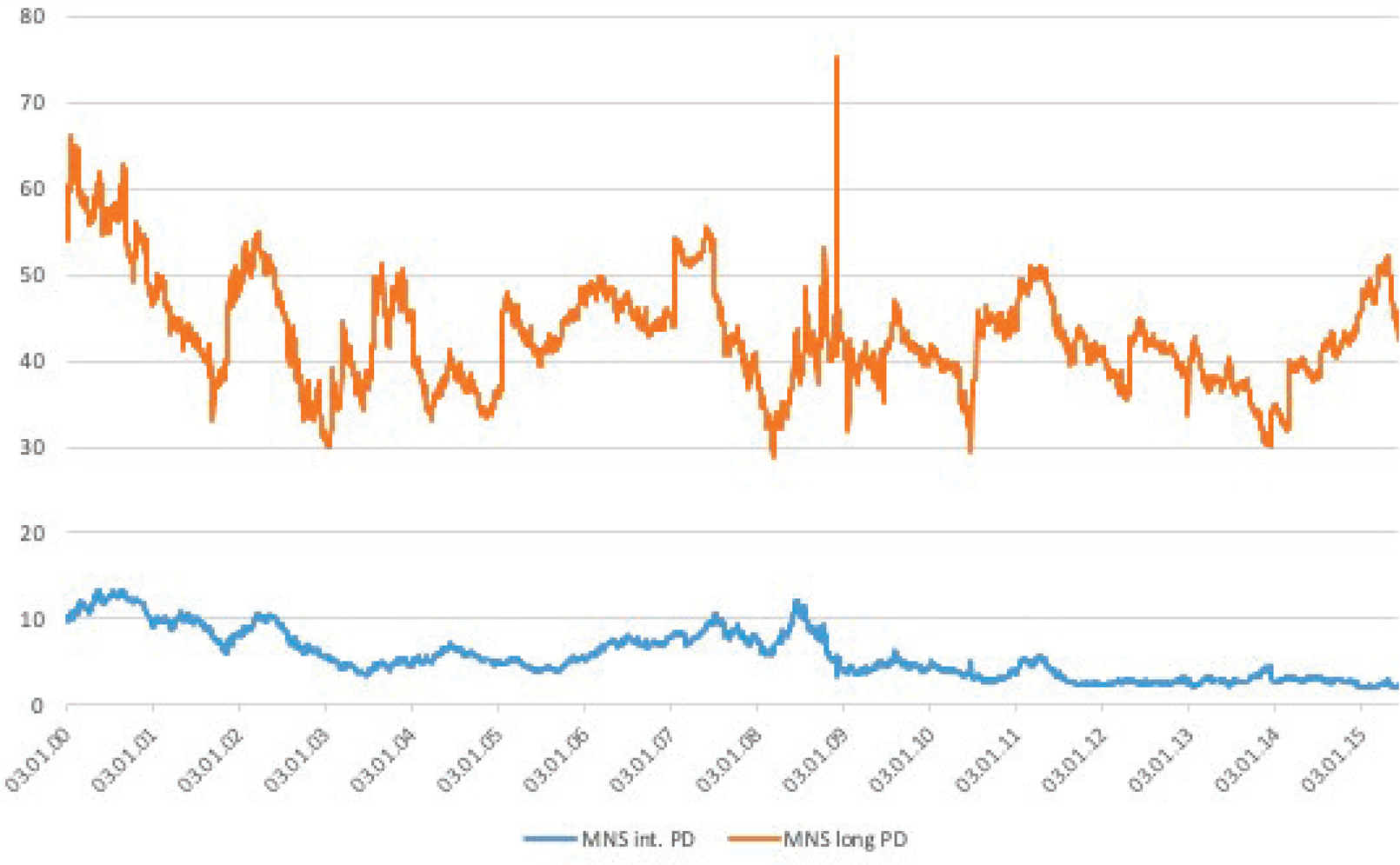
Figure 2. Daily time–series of the MNS PD measures. The figure plots the daily time series of the PD measures for the intermediate (blue) and long (orange) maturity segments of the yield curve, where long bonds are those with maturities longer than 20 years. PD is defined as the root mean squared deviation from the smooth MNS curve fitted on German sovereign notes and bonds with maturities between 6 months and 20 years. For bonds with longer maturities, PD is based on the extrapolation of this smooth MNS curve. All measures are expressed in basis points. The sample spans January 2000 to March 2015, and the data come from Bloomberg.
Panel C of Table 2 allows us to compare the PD measure fitted on German data with the US noise measure from HPW. For this period, the US fitting error was on average 3.06 bps and ranged between 0.73 and 20.47 bps, values that are considerably lower than those of their German counterpart(s). Figure 3 provides a graphical comparison of the intermediate PD measures based on the standard and MNS approaches, respectively, to the noise measure of HPW. The time series comparison also helps to shed more light on the similarities of the time series patterns of these measures. All measures exhibit a large spike around the financial crisis, but the US measure goes back to a level of near zero afterwards, with its German counterparts fluctuating at higher levels. On the other hand, there are slight differences between the standard NS and MNS PD measures: the MNS approach can not only account for the convexity effect, but seem to be less sensitive to periods of high volatility, as its consistently lower values during the Euro-crisis suggest.
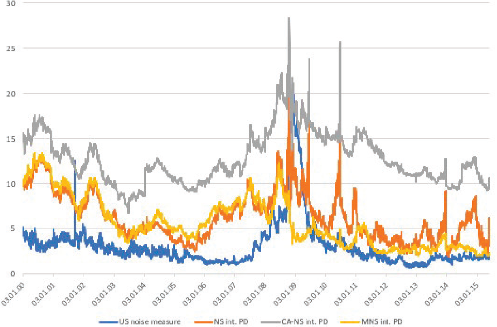
Figure 3. Comparison of the German PD and the US noise measures. The figure compares the time-series of intermediate-maturity PDs and US noise measures. The German PDs are based on the standard NS (orange), the CA-NS (grey), and MNS (yellow) yield curves, while the noise measure (blue) is derived from a Svensson curve of US Treasuries. All measures are expressed in basis points. The sample spans January 2000 to March 2015. The German price data come from Bloomberg, while the noise measure series is obtained from the website of Jun Pan.
Note, however, that contrasting the HPW noise and PD measures is not an ‘apples-to-apples’ comparison, due to their different composition and methodological choices. First and foremost, HPW fit their model to bonds with shorter maturities (less than 10 years), also including a wide range of T-bills in their analysis. Consequently, noise is calculated for a smaller set of bonds and is averaged over the entire US Treasury curve. Our focus, on the other hand, is exclusively on notes and bonds, instruments with longer maturities. For intermediate and longer maturity bonds, we separately calculate the PD measures. For HPW, the use of the Svensson method is suitable as in their selected smaller maturity range the impact of convexity is possibly negligible. In contrast, we resort to the MNS approach, where we can better account for the increasing convexity effects along the the maturity spectrum.
3.2 The bias
The next measure to evaluate the goodness of fit of the various extrapolation methods is based on the average pricing error of long maturity bonds. There are two potential sources of this pricing error: (i) the model choice, and (ii) economic factors that could lead to structural distortions in the different maturity segments. In case of the latter, market segmentation stemming from demand pressures on certain yield segments, differential risk exposures or liquidity, could drive a wedge between the model-implied yields and the ones observed in the market. We call this difference the bias, and define it as follows:

The bias is the average of differences between the observed, $y_t^{{\rm long}, i}$![]() , and model implied yields, y long,i(b t), of bond issues with maturities exceeding 20 years.
, and model implied yields, y long,i(b t), of bond issues with maturities exceeding 20 years.
Panel D of Table 2 reports the descriptive statistics of the bias for the various fitting methods. The statistics suggest that the different methods result in striking differences. While the bias derived from the standard NS approach, is on average is moderately small, about −1.54 bps, with a range close to 100 bps, the CA-NS method delivers a large and positive average bias of about 80 bps, with a similar range. In contrast, the MNS method shows that the bias is persistently negative, on average −38.80 bps, with a smaller range between −75.28 and −19.99 bps.
We depict the bias across the different fitting methods in Figure 4, as well as focusing on the MNS bias across the different long maturity buckets in Figure 5. Figure 4 highlights the importance of the fitting method: the resulting variants of the bias exhibit diverse time series patterns that come with different implications. While the standard NS-based bias is persistently negative in the second half of the sample, it switches sign multiple times in the sample period. In contrast, the bias implied by the CA-NS method is positive throughout, while the theoretically preferred MNS based bias is persistently negative. In Figure 5 we zoom in on the bias along the maturity distribution, where the top panel focuses on the overall bias, while the bottom shows its decomposition into 20–25 and 25 + years maturity buckets. The figure demonstrates that the MNS bias is not only negative in the entire sample period, but this effect is even more pronounced for the longest (25 + years) maturity bucket.
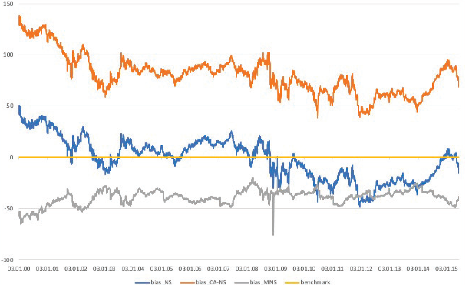
Figure 4. Bias estimates across fitting methods. The figure plots the daily time series of the bias across the different curve fitting methods. The bias is the structural deviation of long maturity bonds, measured as the fitting error of long maturity bonds relative to a smooth curve, which is fitted on German sovereign notes and bonds with maturities between 6 months and 20 years. The methods are the standards NS (blue), the CA-NS (orange), and the MNS (grey) approach, while the benchmark of zero (yellow) is added. All measures are expressed in basis points. The sample spans January 2000 to March 2015, and the data come from Bloomberg.
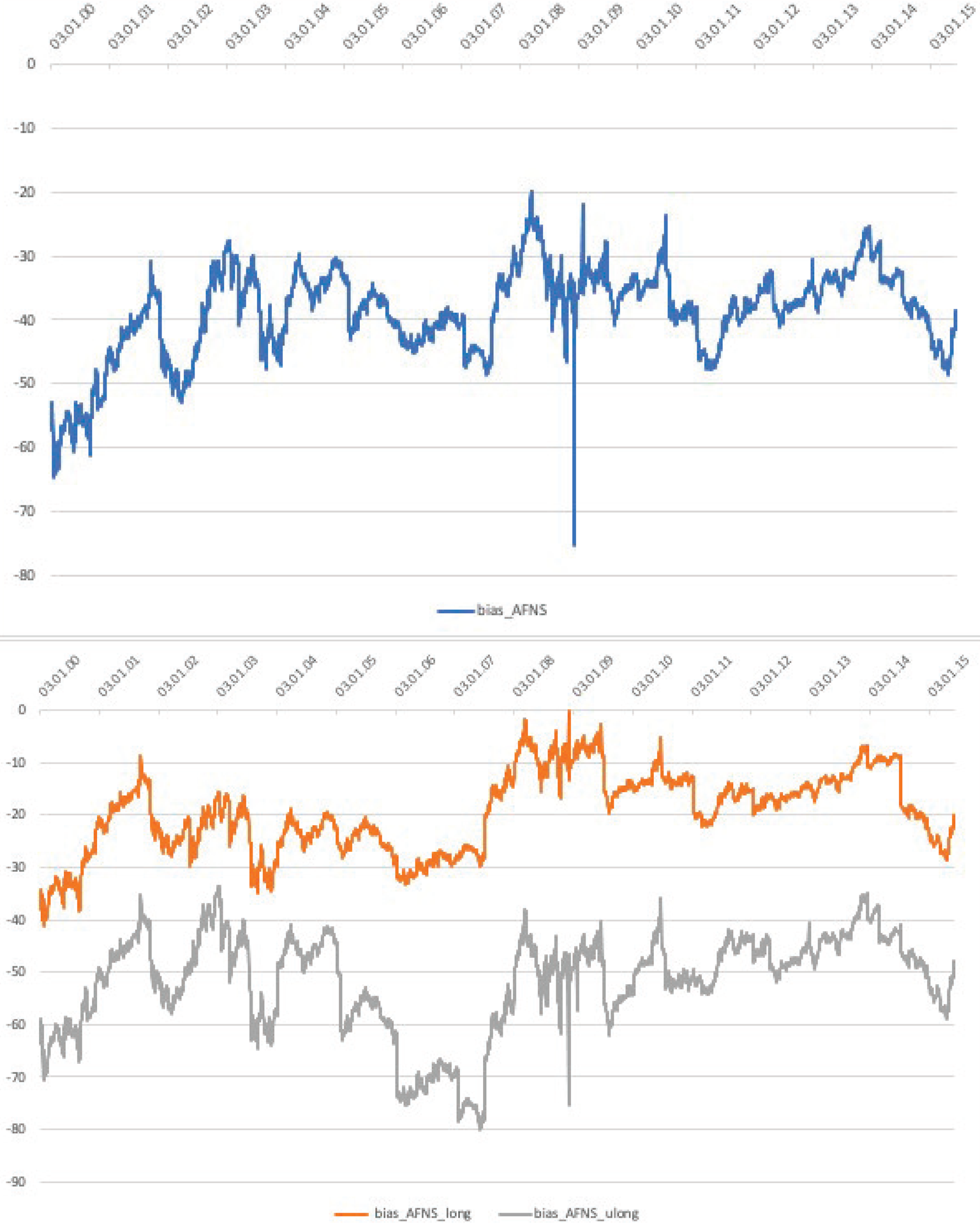
Figure 5. Daily time series of the MNS bias. The upper panel of the figure plots the daily time series of the bias. The bias is the structural deviation of long maturity bonds, measured as the fitting error of long maturity bonds relative to the smooth MNS curve, which is fitted on German sovereign notes and bonds with maturities between 6 months and 20 years. The lower panel plots these fitting errors for two maturity buckets: 20–25 and 25+ years to maturities, respectively. All measures are expressed in basis points. The sample spans January 2000 to March 2015, and the data come from Bloomberg.
It follows from equation (4) that the bias is negative when the observed yields are consistently lower than those implied by our pricing model. We postulate that the bias could be driven by two factors: while we cannot exclude the possibility of some model (fitting) error, unreported analysis shows that the bias is positively correlated with proxies of bond level and general market liquidity, changes in CDS quotes and market volatility. This suggests that the bias is likely the sum of modeling errors, segmentation effects, and some level of liquidity premium. Still, we think it is interesting that, with the relatively simple MNS approach, a bias of −39 bps is achieved, which is economically not very large.
3.3 Robustness tests
In this section we test how sensitive the long maturity PD and the bias measures are to changing the shape parameter of the MNS curve. Due to the poor identification of τ in preliminary unrestricted estimations, in the main analysis we fix it at its the median value (τ = 1.85).Footnote 12 We show below that the size and time series characteristics of the long-term PD measure and the bias are not affected much by the choice of the shape parameter. We focus on measures of the long end as those are ‘out-of-sample’ tests of the curve fit, where using alternative values of τ are expected to be the most pronounced.
The four panels of Figure 6 depict the long-term PD and bias measures resulting from either an unrestricted estimation or from τ fixed at different values. First, we compare the long-term PD and bias measures based on the unrestricted estimation to those where τ is fixed at its unconditional median. The upper panels of Figure 6 show that the unrestricted measure is rather erratic in both cases, but interestingly its fixed-τ counterpart seems to provide an upper bound for long PD, while it appears to be a lower bound for the bias. Another notable feature of the unrestricted measures are the large spikes that they exhibit on days where the optimization is numerically unstable.
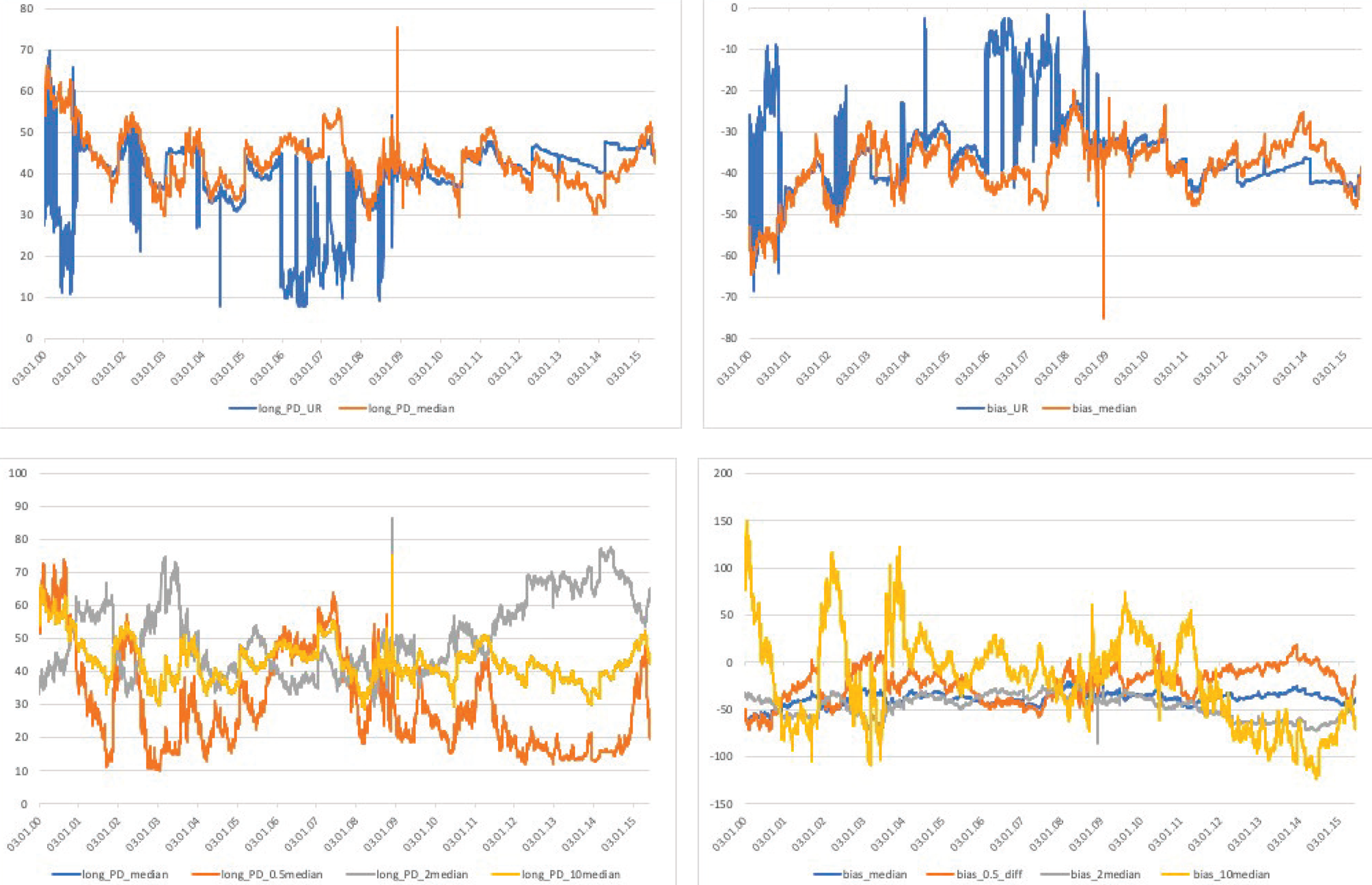
Figure 6. The MNS model's robustness to the choice of τ. The four panels of the figure depict how the choice of tau affects the PD and bias measures of long maturity bonds. We consider different τ parameters from unrestricted and constrained optimization of the MNS curve. The two upper panels compare the long-term PDs and the bias based on unrestricted estimation and another, where taus is fixed at its median value based on the previous method. The lower panels compare the PD and bias measures for different fixed values of τ: half the median, median, twice, and ten times the unconditional median of the parameter. All measures are expressed in basis points. The sample spans January 2000 to March 2015, and the data come from Bloomberg.
To test the extent to which our results are driven by the choice of τ, we re-estimate the PD and bias measures using different fixed levels of τ. These values are the following: half of the median, the median, then twice and ten times the unconditional median estimates of τ. Since τ determines at which maturity the middle-term component of the yield curve reaches its maximum, we believe that our choice of at most twice the median could be economically reasonable values. The lower panels of Figure 6 show that even an unrealistically large parameter value of 18.5 years would not generate PD and bias measures that are magnitudes larger than our benchmark estimate.
4. Policy discussion
This section focuses on three issues. First, we examine the choice of the yield curve that is used for P&I's regulatory liability valuation, comparing the current market practice to the standard NS and MNS curves. This is followed by an ALM case study for two hypothetical pension funds with different characteristics, using the yield curve candidates from the previous section. And lastly, we explain our contribution to the European policy discussion on UFR.
4.1 Yield curve for regulatory liability valuation
How different is the extrapolated (M)NS curve from the one used by regulators? On a more theoretical level, it is a generally interesting question whether (prudential) regulatory valuation should be based on swaps, which are derivatives pension funds and insurers use to hedge their interest rate exposures, or government bonds, which they hold in potentially large quantities in their asset portfolios. For instance, German Pensionkassen and Pensionfonds are allowed to hold government debt up to 50% and 100% of their portfolio value, respectively. As opposed to this, Dutch pension funds do not face such portfolio restrictions.Footnote 13. What the academic literature suggests is that both sovereign bond yields and swap rates could be distorted by various factors and therefore both constitute a noisy proxy for discount rates.
We propose in the paper that long-maturity bond yields might not suffer more significant distortions than swaps, and therefore we suggest their use as an alternative for the construction of the prudential regulatory curve. There is a growing body of research that examines long-maturity swaps and finds that their demand pressure-induced PD s are often comparable to those of long-term government bonds (Klinger and Sundaresan, Reference Klinger and Sundaresan2019; Jansen, Reference Jansen2021, among others). In addition, these swaps are bilateral transactions, not necessarily subject to central clearing, especially in a part of the period that we study, and therefore carry counterparty risk compensation, that, along the business cycle, could be(come) substantially large.
In answering this question, we compare the actual UFR curve, provided to us by the DNB, to the standard NS and MNS curves. The UFR curve is constructed following the guidelines provided by the European Insurance and Occupational Pensions Authority (EIOPA), and it is based on euro-denominated interest rate swap data from Bloomberg. The UFR method is an extrapolation technique to calculate long term discount rates for valuation of liabilities for regulatory purposes, and for maturities beyond the last liquid point.Footnote 14 This point for euro-denominated interest rates is set at 20 years. In practice, this means that the regulatory curve is fitted on interest rate swap rates up to the 20 years to maturity contract, and from that point, it is interpolated between this market rate and the UFR rate at 60-year (or longer) maturity. The UFR rate set at 4.2% at the time of our analysis.Footnote 15 The other curves in this comparison are the NS and MNS curves from Section 2.2.1 and 2.2.3, fitted on German government bond yields up to 20 years-to-maturity, then extrapolated beyond this point.
Figure 7 presents the comparison between the UFR and the extrapolated NS and MNS curves. The upper panel depicts the UFR curve as it has been provided by the DNB, using data for February 23, 2015. It is immediately apparent that fitting the curve on swap rates gives rise to a sizeable spread between the UFR and NS-based term structures.Footnote 16 To adjust for this difference, the lower panel shows the same NS and MNS curves together with the UFR curve net of the swap level premium. The assumption underlying the swap premium correction is that counterparty risk is independent of the contract's maturity. We define the swap premium as the average difference between the NS curve fitted on bond data and the UFR curve based on swap data up to 20 years to maturity.Footnote 17 As a result, the premium-corrected curve is parallel to the original, but shifted downwards so that intermediate UFR and NS yields are fairly similar and deviations for longer maturities reflect differences in the extrapolation. We dedicate the next section to examining how this difference in extrapolation affects P&Is' liability valuation.
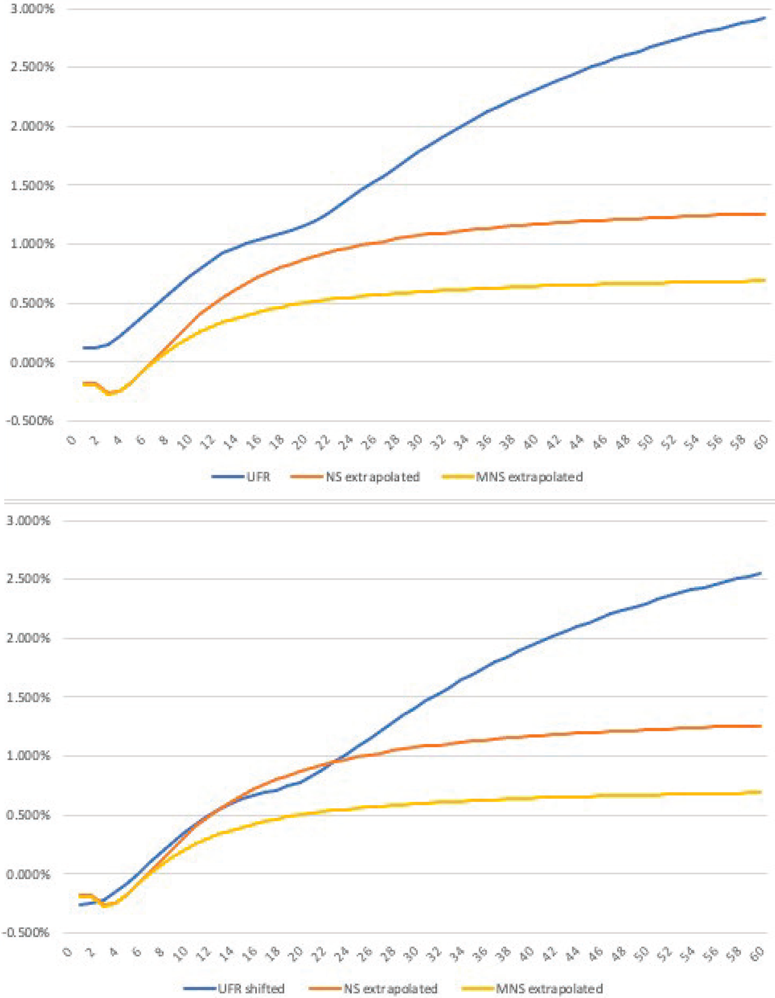
Figure 7. Regulatory vs. (M)NS curves. The figures above depict the yield curve on February 23, 2015. Both panels compare the UFR curve, fitted on interest swap data, to the NS and MNS curves of the study extrapolated beyond 20 years to maturity. The panel above depicts the UFR curve as it has been provided by the Dutch National Bank, while the panel below shows the unchanged NS and MNS curves together with the UFR curve net of the swap premium. The swap premium likely reflects the counterparty risk premium in bilateral swap contracts.
4.2 Liability valuation: a case study
Our aim in this section is to quantify the effect of the aforementioned discount curves on liability valuation of P&Is. We perform this thought experiment by focusing on the curves on the lower panel of Figure 7. We assume that there exist two hypothetical pension funds. Both funds pay out €100 in total over a payment schedule of 60 years. Participants join a fund at the age of 25 and pay a steady stream of equal contributions over the years, until they reach retirement age at 65. From the age of 65, they qualify for a steady stream of pre-defined cash flows until they die at the age of 85.
The two funds differ in their participant composition. The first fund is a large fund with a constant number of participants uniformly distributed between the age of 25 and 85 years. This implies that in each period, the fund has to pay out 1/60 fraction of its total liabilities, thus €1.67. The other fund is a young fund, in which participants' age ranges between 25 and 50 years, while they are in a constant supply. This means that in the first 15 years, the fund does not have any payouts, but as its participants gradually reach retirement age, payouts increase. This increase is linear and lasts until the 35th year of the schedule, when the younger fund also reaches a steady state, in which an equal number of people enter the fund at 25 and leave it at the age of 85. In fact, the main difference between the steady-state and young funds is the duration of their liabilities, which is longer for the young fund. Assuming that the funds hold the same asset portfolio, any difference in their funding ratios would be attributable to differences in their liability duration.
The upper panel of Figure 8 depicts the payout schedule of the two funds, while the lower shows the comparison between the difference in liability values discounted by either the UFR, extrapolated NS or MNS curves. We find that the choice of the discount curve significantly impacts the present values of liabilities. The discounted liability values are substantially smaller when the UFR approach is applied, as opposed to the bond market based NS or MNS curves. The difference in the present values for the steady-state fund is €9.76 or 13.22% with the NS curve, while it is €19.85 and 23.65% relative to the MNS curve. The present value difference is even more sizeable for the younger fund, where the duration of the liabilities is longer: it is €16.20 or 21.94% with the NS curve, while it is €30.89 and 40.45% relative to the MNS curve. Moreover, switching between the UFR and NS and MNS curves not only affects the difference within, but also across funds: discounting by the UFR curve enlarges the present value difference between the young and steady-state funds to €18.62, while it is €12.19 and €7.59 for the NS and MNS curves, respectively.
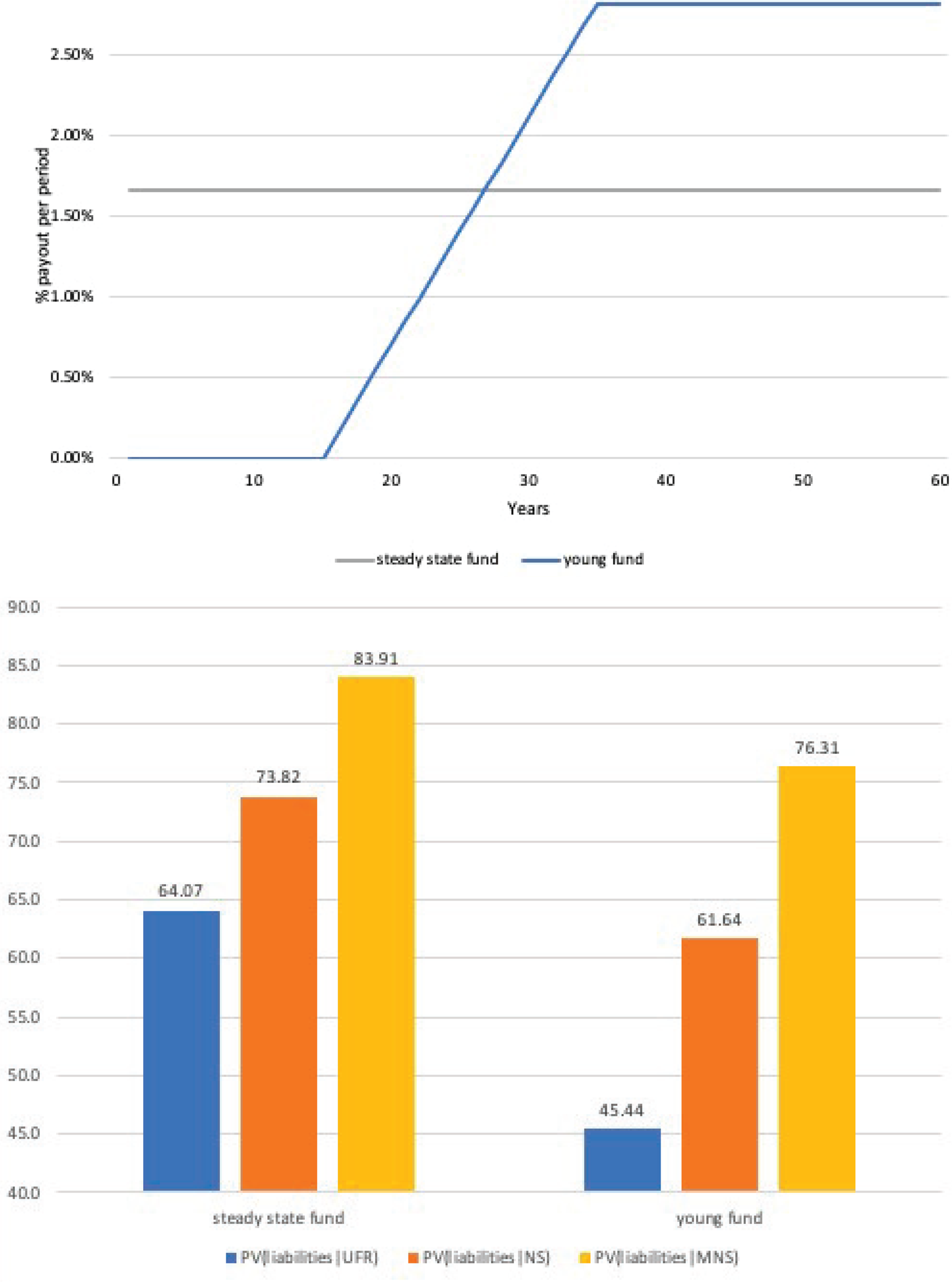
Figure 8. Welfare effects on liability valuation. The figure depicts the liability payout schedules and present values of these liabilities for two hypothetical pension funds: a large and a small and young fund. The upper panel depicts the cash flow structures assumed for the two pension funds in the calculation of welfare effect when one switches from the current regulatory curve to the one we propose for liability valuation. The lower panel compares the present values of liabilities of the two hypothetical funds, where liabilities are either discounted by the shifted UFR or by the extrapolated NS and MNS curves.
Considering the actual size of the difference in and the volatility of the present value, we conclude that the differential effect of the three curves on liability valuation is large. Consequently, the impact on the funding ratio of a typical pension fund can be substantial, potentially similar in magnitude to the variation stemming from the annual fluctuations of funding ratios due to market returns and interest rate changes.Footnote 18 Similar to Christensen et al. (Reference Christensen, Lopez and Mussche2021), we argue that the bond-market based MNS curve is an interesting candidate for liability valuation, nevertheless, using the proposed curve has direct implication on asset and liability management: all else equal, the resulting larger liability values would decrease the funding ratio. While the bond-market based MNS funding ratios are prudentially more desirable, their implementation likely would have hampered regulatory compliance and therefore put P&Is under strain in the persistently low interest rate environment of the past decade.
4.3 Policy discussion and the scope of our contribution
There are three distinct issues regarding the current industry practice that we would like to discuss in this section: (i) how to fit the curve and how to extrapolate beyond the last liquid point; (ii) based on which information should long-term discount rates be determined; and last, (iii) where the last liquid point should be set. While we do not directly address all three of these issues, our results and the pension case study offer suggestions to policymakers and regulators alike.
Firstly, the main contribution of the paper is the extrapolation method, the MNS approach. Our results suggest that the MNS curve fitted on bond market data might be a viable alternative to the UFR method proposed by the Solvency II Directive of the European Commission and EIOPA, similar to the results of J. H. E. Christensen, Lopez, and Mussche (ibid.). This method is not only simple and easy to implement, but it is theoretically appealing: it generates yield curve estimates that are consistent with affine terms structure models, like Christensen et al. (Reference Christensen, Diebold and Rudebusch2011) and Christensen et al. (Reference Christensen, Diebold and Rudebusch2009)'s Arbitrage-Free NS model. Our three-step procedure to fit the MNS curve, based on the convexity adjustment and the re-estimation of the NS parameters from convexity-corrected yields constitutes a significant (computational) shortcut relative to the typical Kalman-filter based maximum-likelihood estimation of the said models. This ease of implementation makes our method an attractive alternative to put in practice by P&Is.
Secondly, there is the question of whether bond or interest rate swap data should be used for regulatory valuation purposes. Both interest rate swaps and government bonds are important assets in P&Is' portfolios, albeit they are held for different purpose: while swaps help hedging interest rate risks, government bonds constitute the backbone of many fixed-income portfolios. What the various literature strands tell us, however, is that both sovereign bond yields and swap rates could be distorted by various factors, and therefore both constitute a noisy proxy for discount rates. While conceptually the use of (near) default risk free government bonds could be preferable, the liquidity of swaps and the possibility to trade maturities that extend beyond those issued by governments are certainly beneficial. On the one hand, the liquidity of swaps could have been potentially offset by their counterparty risk exposure, with the proliferation of central clearing of these products, standard contracts that qualify to be cleared, carry significantly lower counterparty risk premiums than in the past. In practice risk premiums might be small, however, a growing body of research shows that long-maturity swaps suffer from demand pressure-induced PD s, that are often comparable to those of long-term government bonds (Klinger and Sundaresan, Reference Klinger and Sundaresan2019; Jansen, Reference Jansen2021). On the other hand, bonds yields have been shown to contain a convenience yield (Krishnamurthy and Vissing-Jorgensen, Reference Krishnamurthy and Vissing-Jorgensen2012), some of which has eroded over time and especially in periods of crises (Klingler and Sundaresan, Reference Klingler and Sundaresan2020; He et al., Reference He, Nagel and Song2022). The stable part of the convenience yield is, nonetheless, likely driven by periodic demand factors, like repo market specialness (Duffie, Reference Duffie1996), central bank collateral eligibility (Pelizzon et al., Reference Pelizzon, Riedel and Simon2020), or cheapest-to-deliver status on the CDS and futures markets (Pelizzon et al., Reference Pelizzon, Subrahmanyam and Tomio2020). One can conclude that overall, from a regulatory perspective there are both advantages and disadvantages of relying only on information from a single market. Future work should explore the possibility of models that have the capacity to integrate information from both bonds and swaps, but for now, this topics remains beyond the scope of our paper.
And last, we enrich in part the discussion about the LLP. There is an open debate on where this point should be set. While EIOPA and the Netherlands uses 20 years for the division point, in Sweden the last liquid point is set at 15 years to maturity. Though specifically testing how robust (any) extrapolation method to the location of the LLP is of clear regulatory interest, this is a question largely left unanswered by the literature in financial economics. However, the empirical evidence from Greenwood and Vissing-Jorgensen (Reference Greenwood and Vissing-Jorgensen2018), Klinger and Sundaresan (Reference Klinger and Sundaresan2019), or Jansen (Reference Jansen2021) indicate that both bond and swap markets shows signs of demand pressure generated by prudential regulation. These effects prove that P&Is' ALM practices have an economically significant impact on both swap and bond markets around and likely even beyond the LLP.
What would happen if the regulator moved this point along the swap curve, or relied on the bond market instead? A related aspect is how regulatory pressure would impact the underlying markets. Our understanding is that EIOPA resorted to the UFR method since the long-end of the swap curve was considered too illiquid to serve as a benchmark. It is an interesting question whether a negative (liquidity) feedback would affect the pricing of very long-term government bonds if those are used more for regulatory purposes. Studying this goes beyond the scope of our paper, since it would require some estimate of the price impact of ‘additional’ trading in long-term government bonds, and an estimate of how much additional demand for long-term bonds would be generated. Many long-term investors already hold a substantial part of the long-term bond supply for their internal ALM, and it is thus not easy to estimate how much additional regulatory-driven demand would occur if the benchmark method were changed.
5. Conclusion
This paper presents a simple yield curve extrapolation technique that produces discount rates suitable for regulatory valuation. This technique is not only easy to implement due to its few estimable parameters, but it also relies on prices of government bonds traded on the market. The resulting method, the MNS curve is theoretically appealing as it is consistent with arbitrage-free affine term-structure models, like the Arbitrage-Free NS model (Christensen et al., Reference Christensen, Diebold and Rudebusch2009, Reference Christensen, Diebold and Rudebusch2011).
Next, we study how well the MNS curve fits the data. Specifically we fit the MNS curve, incorporating a convexity adjustment, to bonds with remaining maturities between 6 month and 20 years, while for longer maturities we use this smooth curve for extrapolation. This specific approach is inspired by the UFR method's choice of the last liquid point and therefore provides extrapolated yields that are comparable to the regulatory curve – an exercise that we perform in the last section of the paper.
We evaluate the goodness of fit of our extrapolation methods by studying two measures: the PD and bias measures. We calculate the PD measure as the root mean squared pricing error relative to the smooth MNS curve, and calculate it for intermediate (in-sample) and long (out-of-sample) maturities. The bias, on the other hand, is based on the average pricing error of long maturity bonds. We find that both the PD and bias measures are reasonably small in our sample of German government bonds between January 2000 and March 2015. We postulate that there could be two potential sources of these pricing errors: (i) the model choice resulting in small model-driven fitting errors, or (ii) economic factors that could lead to structural distortions in the different maturity segments of the yield curve. In case of the latter, market segmentation stemming from demand pressures on certain yield segments, differential risk exposures or liquidity premiums, could drive a wedge between the model-implied yields and the ones observed on the market.
Lastly, we provide a detailed policy discussion on the European regulatory liability valuation procedure, the UFR method. The UFR is an extrapolation technique to obtain long term discount rates beyond the LLP. We compare the UFR curve based on interest rate swap data and the guidelines of EIOPA, to the standard NS and MNS curves. Next, we expand this comparison in a simple case study that evaluates the liability valuation properties of these curves. We conclude our discussion by reflecting on the current regulatory practice, with respect to its choice of extrapolation technique, use of bond versus interest rate swap data, and the LLP and its potential impact along the (yield) curve.
Acknowledgement
We would like to thank Anne G. Balter (discussant), Dion Bongaerts, Paolo Colla (discussant), Frank de Jong, Daniel Havran (discussant), Stefan Ruenzi and the conference and seminar participants of the Summer Workshop of the Hungarian Academy of Sciences, the 7th Annual Financial Market Liquidity Conference, the 2017 Netspar International Pension Workshop, the German Finance Agency, the 2017 FMA Boston, and the Securities Markets: Trends, Risks, Policies conference by Consob-Bocconi for valuable comments and feedback. The previous version of the paper was circulated under the title ‘Much ado about nothing: A study of differential pricing and liquidity of intermediate and (ultra-)long term bonds’. We are responsible for all remaining errors.
Conflict of interest
Driessen and Nijman have nothing to declare. Simon gratefully acknowledges research support from the Leibniz Institute for Financial Research SAFE, and has nothing further to declare.
Appendix
A. The German sovereign bond market
The Federal Government of Germany is one of the largest issuer of government securities in the Eurozone. These securities are not only highly liquid, but they also carry small issuer risk and preserved their AAA rating even during the height of the Euro crisis. German government bonds have maturities from 6 months to 30 years, which span the entire yield curve with 60–70 tradeable securities at any point in time. Capital market securities consist of three types: Federal Treasury notes (Schaetze), Federal notes (Bobls) and Federal bonds (Bunds) with the maturities of 2, 5, and 10 or 30 years, respectively.Footnote 19
German sovereign bonds are typically placed to bidding group members, similar to U.S. primary dealers, in the form of single issues via auctions. These can be followed by multiple re-openings to keep the market liquid and to facilitate the delivery of futures contracts and other instruments written on these bonds. The average outstanding volume of a single issue is around €15–20 billion. According to the German Treasury, the relative share of each security type is stable over time: 2-year notes constitute 9%, 5-year notes 21%, 10 years Bunds 44,5% and 30 year Bunds 17% of the overall public debt issued by the Federal Government in 2015. This means that our sample covers about 90% of all German tradeable government debt (stock), and about 70% of the total issuance (flow). All capital market securities have fixed maturities with redemption on maturity at the full nominal value, as well as annual fixed interest payments. The high liquidity of these bonds is assured by repo-, and ECB collateral-eligibility irrespective of their maturity, while Bunds are even stripable.Footnote 20
The above features highlight why we chose to study the regulatory curve in Germany. Its nominal bond market not only serves as the benchmark Eurozone sovereign bond market, but arguably, it is the closest to being free of default risk in our sample period. While there are other large and liquid sovereign markets in Europe, such as Italy or France, the additional risk premiums in those bond yields (default risk, Euro-breakup risk, etc.) may distort the analysis. Hence, the dynamics of these yields do seem to contain such additional factors, which makes it harder to model and interpret the curves from these countries. Overall, in Germany, due to its large and liquid bond market, the hypothesized distortions are likely to be small, since market liquidity facilitates arbitrage and thereby keeps asset prices close to fundamentals. In fact, this market is relevant from the regulatory perspective and applications, as it provides a lower bound for these distortions in the Eurozone. Furthermore, beyond being the benchmark economy, Germany is also a safe haven market in the euro area. At the same time, a harmonized prudential regulatory reform affecting the natural clientele of intermediate and long maturity bonds also takes place in the studied period.Footnote 21
B. Convexity correction
This appendix provides the detailed steps to calculate the convexity correction explained in Section 2.2.2.
To apply the convexity correction, one has to estimate a VAR(1) process of the level (β 0), slope (β 1), and curvature (β 2) parameters of the NS model. We implement the model below using end-of-month parameter values from the initial NS estimation, following the description in Section 2.2.1:

where the vector of errors, ei,t, has a zero mean and a diagonal variance matrix with variance equal toΔt. Estimating the VAR(1) process in equation (B.1) results in the following volatility matrix, Σ:

Using this volatility matrix, the convexity correction takes the following form:
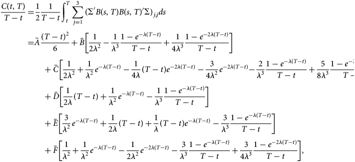
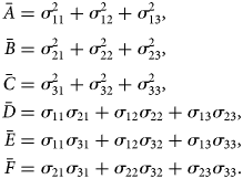
where λ = (1/τ), where τ is the shape parameter of the NS curve.$\bar{A}$![]() , $\bar{B}$
, $\bar{B}$![]() , $\bar{C}$
, $\bar{C}$![]() , $\bar{D}$
, $\bar{D}$![]() , $\bar{E}$
, $\bar{E}$![]() and $\bar{F}$
and $\bar{F}$![]() are defined by the following expressions:
are defined by the following expressions:
C. Extended pension case study
This appendix presents further results of the pension case study, where Figures 7 and 8 are expanded by various swap premium adjusted UFR curves. We model the swap premium either as constant, that is, with a flat term structure, or by an increasing premium (at a different but) constant rate beyond the the 20-year cut-off, the LLP.
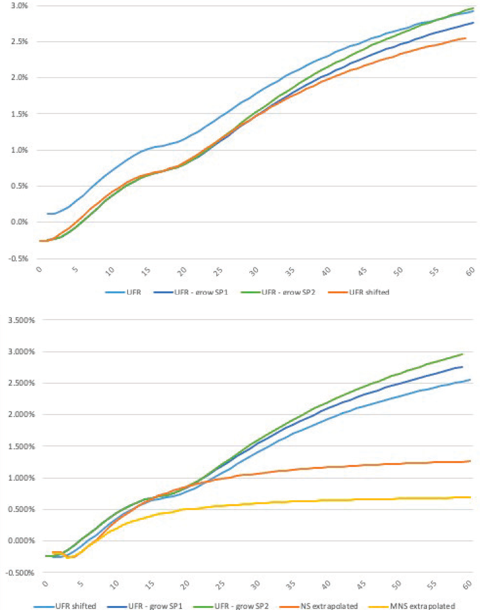
Figure C1. Swap premium adjusted regulatory vs. NS curves. The figures above depict the yield curve on February 23, 2015. The top panel compares the UFR curve, fitted on interest swap data, against versions of the same curve net of the swap premium. The swap premium likely reflects the sum of compensation for counterparty risk in bilateral swap transactions and illiquidity of certain contracts, and is modeled in three different ways: the curve denoted as ‘UFR shifted’ assumes a constant swap premium, while ‘UFR-SW1’ and ‘UFR-SW2’ are based on a premium that increases at a constant rate beyond the last liquid point, by 0.5 and 1 bps per annum, respectively. The lower panel depicts the three swap-premium adjusted curves to the unchanged NS and MNS curves.

Figure C2. Welfare effects of liability valuation. The figure depicts the liability payout schedules and present values of these liabilities for two hypothetical pension funds: a large and a small and young fund. The cash flows are identical to those in Figure 8, while the lower panel compares the present values of liabilities of the two hypothetical funds, where liabilities are either discounted by the shifted UFR, UFR-SW1 (0.5 bps/p.a. increase beyond the LLP), UFR-SW2 (1 bp/p.a. increase beyond the LLP) or by the extrapolated NS and MNS curves.

