


1 Introduction
A pipe flow can stay laminar at any arbitrarily large value of Reynolds number ( $Re$). But, if finite-amplitude perturbations are present, other flow states come into being for $Re\gtrsim 1600$. (Here, $Re\equiv UD/\unicode[STIX]{x1D708}$, where $U$ is the mean flow speed, $D$ is the pipe diameter and $\unicode[STIX]{x1D708}$ is the kinematic viscosity of the fluid.) When the value of $Re$ is smoothly increased, patches of intense eddies suddenly appear and invade the laminar flow, creating a heterogeneous blend of fluctuations and quiescence. In 1883, Osborne Reynolds first observed these travelling patches of eddies and called them ‘flashes’ (Reynolds Reference Reynolds1883). Since then, scores of experiments (see, e.g. Mullin (Reference Mullin2011) for a review) have elucidated a growing list of fascinating features of flashes. For example, low- $Re$ flashes can remain of fixed size, split to form new flashes or decay into laminar flow, whereas high- $Re$ flashes expand. This led to the categorization of flashes into ‘puffs’ ( $1600\lesssim Re\lesssim 2250$) and ‘slugs’ ( $Re\gtrsim 2250$), which can expand as well as split ( $2250\lesssim Re\lesssim 2700$) or monotonically expand ( $Re\gtrsim 2700$).
A puff travels downstream at a speed  ${\approx}0.9U$ (Mullin Reference Mullin2011). The laminar flow enters the puff at its upstream interface, turns into fluctuating flow and exits at its downstream interface, reverting to laminar flow. This fluctuating flow evolves over the whole length of the puff, never reaching a fully developed state – the flow appears to be distinct from fully turbulent flow (see, e.g. Van Doorne & Westerweel Reference Van Doorne and Westerweel2007; Song et al. Reference Song, Barkley, Hof and Avila2017). (Here we define fully turbulent flow to mean fluctuating flow that fills the whole pipe without any intervening regions of laminar flow; further, its statistical properties are independent of axial position, i.e. the flow is fully developed.)
As a slug travels downstream, its upstream interface travels at a speed  ${<}U$ and the downstream interface at a speed ${>}U$, which causes the slug to continually expand. (The speeds of the interfaces systematically change with $Re$.) At the upstream interface, the laminar flow enters the slug near the wall, turns into fluctuating flow, reverses direction and exits the same interface near the centreline, reverting to laminar flow. (Likewise, at the downstream interface there is a recirculating flow, but it is reversed in direction compared with the flow at the upstream interface.) Inside the slug, the fluctuating flow spreads over an ever-expanding domain. This flow inside the slug – slug flow – is the subject of our study.
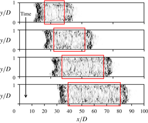
Contrasting slug flow and fully turbulent flow: (a) transitional flow with a slug; (b) fully turbulent flow. We plot a grey scale intensity map (where darker shares correspond to higher intensity) of the kinetic energy of off-axis fluctuations in an  $x{-}y$ (axial–wall-normal) plane through the pipe centreline; the white regions are devoid of fluctuations and correspond to laminar flow. The data are from our simulations at $Re=5300$ (see § 2). A slug (a) travels downstream and continually expands into the surrounding laminar flow, whereas in a fully turbulent flow (b), the fluctuating flow fills the whole pipe. Note that a monotonically expanding slug, regardless of how large the value of $Re$ is, cannot completely fill a pipe with fluctuating flow since it continuously travels downstream, leaving laminar flow behind. (However, for simulations with periodic boundary conditions, owing to the artificial set-up of the problem, a slug eventually fills the pipe with fluctuating flow.) We compare slug flow (schematically marked by rectangular boxes in a) with fully turbulent flow (b; here the box spans the whole pipe).

We focus on  $Re\gtrsim 2700$. In the presence of finite-amplitude perturbations, the flow assumes one of two states: transitional with slugs (when the perturbations are applied intermittently) or fully turbulent (when the perturbations are applied continually); see figure 1. But are these two states fundamentally distinct? For slugs, the recirculating flow near the interfaces is clearly distinct from fully turbulent flow. But, in the interior of a slug, if the slug flow becomes fully developed and is unaffected by the flow at the interfaces, it could be indistinct from – even identical to – fully turbulent flow. Or, it could be distinct from fully turbulent flow, corresponding to a unique state of fluctuating flow. That is, at the same $Re$, the flow may manifest multiple states of fluctuating flow, as indeed has been observed for puff flow and low- $Re$ slug flow (Darbyshire & Mullin Reference Darbyshire and Mullin1995; Mullin Reference Mullin2011), and, more recently, for high- $Re$ turbulent Taylor–Couette flow (Huisman et al. Reference Huisman, Van Der Veen, Sun and Lohse2014). Which of these two possibilities holds determines the statistical nature of fluctuations in slug flow. Based on the pioneering exposition of Wygnanski & Champagne (Reference Wygnanski and Champagne1973), hereafter WC, the former possibility is widely thought to hold true. By comparing slug flow with fully turbulent flow using several diagnostic profiles for the spatial structure of the flow, WC concluded: ‘the structure of the flow in the interior of the slug is identical to that in a fully developed pipe flow’.
Most reviews of the field (see, e.g. Eckhardt et al. Reference Eckhardt, Schneider, Hof and Westerweel2007; Barkley Reference Barkley2016) appeal to this definitive conclusion and recent models of the transition build on it as well (Barkley et al. Reference Barkley, Song, Mukund, Lemoult, Avila and Hof2015; Barkley Reference Barkley2016). Although scarce, some recent works have also studied the same diagnostic profiles as WC (Shan et al. Reference Shan, Ma, Zhang and Nieuwstadt1999; Priymak & Miyazaki Reference Priymak and Miyazaki2004) and echoed the same conclusion. In addition, recent studies using other diagnostics have furnished further support for this conclusion: the friction in slug flow (that is, the unitless pressure drop per unit length of slugs) is found to obey the Blasius law, a signature macroscopic diagnostic of fully turbulent flow (Cerbus et al. Reference Cerbus, Liu, Gioia and Chakraborty2018); and the energy spectra in slug flow is found to conform to Kolmogorov’s small-scale universality, a signature microscopic diagnostic of fully turbulent flow (Cerbus et al. Reference Cerbus, Liu, Gioia and Chakraborty2017). (For transitional flow with slugs, the slug flow and the surrounding laminar flow share the same  $Re$, but the friction in slug flow obeys the Blasius law whereas the friction in laminar flow obeys the Hagen–Poiseuille law (Cerbus et al. Reference Cerbus, Liu, Gioia and Chakraborty2018).) To wit, slug flow and fully turbulent flow appear to be the same flow state.
And yet, a re-examination of WC’s evidence undermines this widely accepted conclusion.
1.1 A close look at WC’s evidence for slug flow = fully turbulent flow
WC reported the results of their extensive experimental study comparing slug flow and fully turbulent flow. These experiments are very challenging, particularly for slug flow – slugs incessantly travel and expand, which makes the probing of their interior a non-trivial undertaking. It is also noteworthy that because WC were able to maintain laminar flow in their pipe until an impressive  $Re\approx 45\,000$, which still surpasses most modern experiments (Mullin Reference Mullin2011), they were able to examine slugs over a wide range of $Re$. WC, a veritable tour de force, remains unmatched as the most comprehensive study to date that compares slug flow and fully turbulent flow.
WC studied the following diagnostic profiles: mean-velocity profiles (MVPs), root-mean-square of fluctuating-velocity profiles (r.m.s. profiles) and Reynolds stress profiles. The guiding principle is that, if the profiles for slug flow are identical to those for fully turbulent flow, then the flows are identical. But, in WC’s study, because the different profiles correspond not only to different flows but also to different  $Re$, the variation in $Re$ needs to be explicitly accounted for. To that end, WC rendered the profiles unitless. Thus, WC’s conclusion that slug flow and fully turbulent flow are identical is predicated on the attendant unitless profiles collapsing onto a common curve.
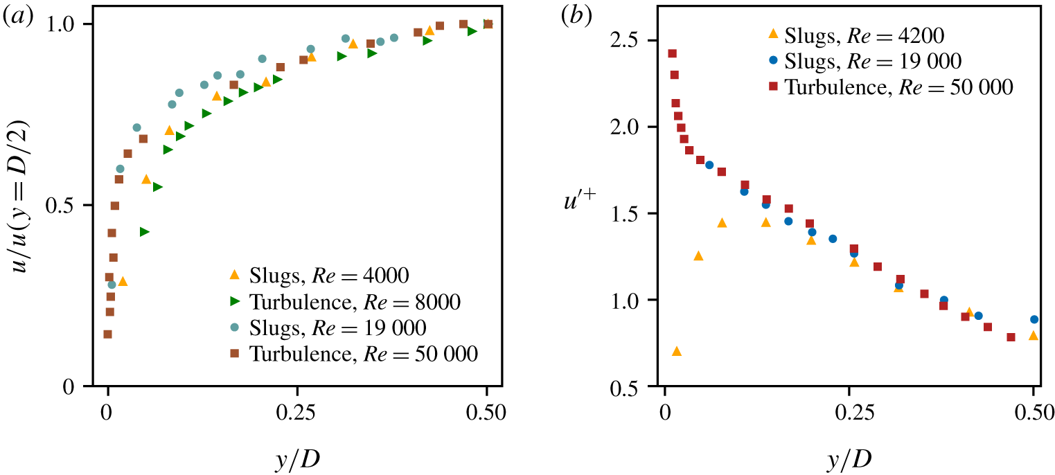
In figure 2, we plot WC’s data for MVPs and r.m.s. profiles in the unitless coordinates adopted by WC. (We discuss the Reynolds stress profiles in § 4.3.) At each wall-normal distance,  $y$, we denote the time-averaged velocity by $u$ and the r.m.s. of velocity fluctuations by $u^{\prime }$. To render the profiles unitless, WC normalized the abscissae as $y/D$, and the ordinates as $u/u(y=D/2)$ for the MVPs and $u^{^{\prime }+}\equiv u^{\prime }/u_{\unicode[STIX]{x1D70F}}$ for the r.m.s. profiles (where $u_{\unicode[STIX]{x1D70F}}\equiv \sqrt{\unicode[STIX]{x1D70F}_{w}/\unicode[STIX]{x1D70C}}$ is the friction velocity, $\unicode[STIX]{x1D70F}_{w}$ is the wall stress and $\unicode[STIX]{x1D70C}$ is the density of the fluid). There is considerable scatter in the data, and it is difficult to argue that the profiles collapse. In discussing their data, WC postulated reasons for the scatter, e.g. influence of the interfaces (see § 3) and ‘experimental error’ (p. 301 in WC). The gist of their argument is that, but for these artefacts, the profiles would collapse. This brings us to the core problem with WC’s analysis: even if the profiles unequivocally showed collapse, it would be incorrect to conclude that the corresponding flows are identical.
Representative diagnostic profiles from WC. (a) MVPs:  $u/u(y=D/2)$ versus $y/D$ (cf. figure 16 in WC) and (b) r.m.s. profiles: $u^{^{\prime }+}$ versus $y/D$ (cf. figure 17 in WC). WC measured ensemble-averaged profiles for slug flow at a distance of $20D$ from the interfaces. Here, we show results for the profiles near the upstream interface; the profiles near the downstream interface are similar. There is considerable scatter in the data: the MVPs, near the wall, show large variation; the r.m.s. profiles for slug flow (at $Re=4200$) and fully turbulent flow are not only distinct but, near the wall, show opposite trends. (WC did not report error bars, so we cannot evaluate whether the scattered data lie within the experimental error.)
To understand why, consider how the profiles are rendered unitless. The underlying theoretical framework for how the profiles change with  $Re$ is furnished by scaling laws. For the MVPs, WC’s choice, $u/u(y=D/2)$ versus $y/D$, is at odds with the classical scaling laws. Further, the scaling laws themselves break down for the typical $Re$ of slug flow (see § 4.1). For the r.m.s. profiles, there are no standard scaling laws, but WC’s choice, $u^{^{\prime }+}\equiv u^{\prime }/u_{\unicode[STIX]{x1D70F}}$ versus $y/D$, is at odds with empirical data (see § 4.2). In other words, the very premise on which WC’s analysis of MVPs and r.m.s. profiles is predicated cannot be used to compare flows at different $Re$. In fact, if the profiles of figure 2 manifested collapse, that would signal a problem, not a solution.
We submit that WC’s conclusion – slug flow is identical to fully turbulent flow – warrants a re-examination. Of crucial import in comparing slug flow and fully turbulent flow is to properly account for the  $Re$-dependence of the profiles. This accounting guides our re-examination. Specifically, we argue that the profiles for slug flow and fully turbulent flow must be compared at the same $Re$ (see § 4). Because such data are not available – in WC or, to our knowledge, any other study – we conduct our own experiments and numerical simulations.
2 Experimental and numerical set-up
Our experimental set-up is a gravity-driven, recirculating flow of water through a smooth, cylindrical, horizontal pipe of inner diameter  $D=2.5~\text{cm}\pm 10~\unicode[STIX]{x03BC}\text{m}$. The pipe is 20 m long, made of 1 m long cylindrical glass tubes connected using acrylic connectors, which also have an inner diameter of $D=2.5~\text{cm}\pm 10~\unicode[STIX]{x03BC}\text{m}$. Several of these connectors have holes of diameter 1 mm, which serve as pressure taps or as an injection point for a perturbation. The flow begins at a reservoir tank whose height we adjust to set the pressure head, which, in turn, sets the flow rate. To further control the flow rate, we use a ball valve at the exit of the reservoir and a ball valve at the end of the pipe. After exiting the reservoir, the water passes through a heat exchanger, which maintains a constant temperature (typically $23.5\pm 0.1\,^{\circ }\text{C}$) and then a Yokogawa magnetic flowmeter, which measures the flow rate $Q$. From $Q$, we compute the mean flow speed, $U=Q/\unicode[STIX]{x03C0}(D/2)^{2}$, and from $U$, we compute $Re$. We conduct experiments for $Re=3000,4000,5300$ and $8000$. After the flowmeter, the flow enters the pipe via an entrance section, which homogenizes and smoothens the flow. The largest pressure drop occurs in the segments before the pipe and in a smaller diameter section we place at the end of the pipe; consequently, the fluctuations in $Re$ during the transition are typically ${<}1\,\%$. At the end of the pipe the water exits into a discharge tank. We pump the water back to the reservoir tank, completing the flow circuit. Without any external perturbation, the flow can remain laminar up to $Re\approx 10\,000$.
We perturb the flow by injecting and withdrawing fluid in the radial direction using syringes. At a fixed  $Re$, we generate a pair of flows: fully turbulent (for which we perturb the flow continually) and transitional with slugs (for which perturb the flow intermittently). At distances ${>}100D$ downstream from the perturbations, we measure the velocity fields using particle imaging velocimetry (PIV). To that end, we use a 5 W, 532 nm laser (FK-LA5000, Omicron) and a series of lenses to form a vertical laser sheet. The sheet pierces the top of an acrylic encasement filled with water (in which the measurement section of the pipe is housed to reduce optical distortion). Straddling the centreline of the pipe, the sheet effects a measurement volume of ${\approx}1D~(\text{radial})\times 0.7D~(\text{axial})\times 0.03D~(\text{thickness})$ and illuminates the flow, which we seed with $10~\unicode[STIX]{x03BC}\text{m}$ silver-coated, density-matched glass particles. For the PIV measurements, we record the movement of the particles using a high-speed camera (Phantom v1610) with 12-bit dynamic range at a resolution of $768\times 512~\text{pixels}$. We optimize the conditions for maximum spatial resolution, while following standard operating procedure for particle displacement and density (Adrian & Westerweel Reference Adrian and Westerweel2011). We take the particle images in double-burst mode, with a pair of images taken at 100 Hz. The temporal spacing between the images in each pair is of the order of 1 ms, which we modify for each $Re$ such that the particles move $5{-}10~\text{pixels}$. We process the images using PIVLab (Thielicke & Stamhuis Reference Thielicke and Stamhuis2014). Each image pair yields one velocity field – a vertical plane through the pipe centreline that spans an area ${\approx}1D~(\text{radial})\times 0.7D~(\text{axial})$ and consists of axial and radial velocity vectors. (We use cylindrical coordinates, with the origin on the centreline of the pipe and $x$ as the axial direction, $r$ as the radial direction and $\unicode[STIX]{x1D703}$ as the azimuthal direction.)
We compute the diagnostic profiles from an ensemble of velocity fields at a fixed  $Re$. For a fully turbulent flow, we measure the fields over a long time (typically, a few $1000D/U$); for a transitional flow with slugs, we measure the fields for several passing slugs (each of typical length from a few $100D$ to about $1000D$). (In both flows, the number of statistically independent fields – that is, fields separated in time by several turnover times, $D/U$ – is typically ${\gtrsim}300$.) For a fully turbulent flow, we compute the diagnostic profiles by averaging the profiles over the axial extent of each field and averaging those profiles over all the fields in the ensemble; for a transitional flow with slugs, we discuss the process in § 3.
We complement our experiments with direct numerical simulations (DNS), using the hybrid spectral code openpipeflow (Willis Reference Willis2017). The pipe is  $100D$ long and we impose periodic boundary conditions in the axial direction. We run the simulations for a fixed mass flux; this sets the value of $Re$. As in the experiments, we conduct simulations for $Re=3000,4000,5300$ and $8000$. Along the $x$ and $\unicode[STIX]{x1D703}$ directions, we use Fourier modes. Along the $r$ direction, we distribute the grid points according to the roots of a Chebyshev polynomial (which places a larger density of points near the wall to resolve the large velocity gradients) and we use finite differences to compute derivatives. As an example of the spatial resolution, consider the DNS at $Re=8000$: we used $8192$ and $168$ modes in the $x$ and $\unicode[STIX]{x1D703}$ directions, respectively, and $180$ points in the $r$ direction. Elsewhere (Cerbus et al. Reference Cerbus, Liu, Gioia and Chakraborty2018) we have verified that our spatial resolution is sufficiently high to produce accurate results (see also figures 8, 9 and 12, where we compare the diagnostic profiles from our simulations with those from Wu & Moin (Reference Wu and Moin2008)).
We start a simulation by choosing an appropriate velocity and pressure field as the initial condition. As in the experiments, at each  $Re$, we generate a pair of flows. To obtain a fully turbulent flow, we use the result of a simulation, at the same or different $Re$, of a fully turbulent flow; to obtain a transitional flow with slugs, we use the result of a simulation, at a different $Re$, of a transitional flow with puffs or a transitional flow with slugs. We select fields separated in time by several $D/U$ and, for each snapshot, we average the fields along the $x{-}r$ planes corresponding to $\unicode[STIX]{x1D703}=0,\unicode[STIX]{x03C0}/4,\unicode[STIX]{x03C0}/2,$ and $3\unicode[STIX]{x03C0}/4$. The ensemble consists of these averaged planes of velocity fields with all three components of the velocity vector. For fully turbulent flow, we compute the diagnostic profiles using the same procedure as described above for the experimental data. For transitional flow with slugs, we restrict attention to cases where: (i) the slugs expand at a steady rate (that is, the speeds of the upstream and downstream interfaces are constant), which typically occurs for slugs of length ${\gtrsim}30D$, and (ii) the maximum length of the slug is $80D$ (to ensure that the slug flow statistics are unaffected by the length of the pipe). With these constraints, the typical number of statistically independent fields in an ensemble for a transitional flow with slugs is typically ${\gtrsim}100$. From this ensemble, we compute the diagnostic profiles (see § 3).
See Cerbus et al. (Reference Cerbus, Liu, Gioia and Chakraborty2017, Reference Cerbus, Liu, Gioia and Chakraborty2018) for additional details about the experiments and DNS.
3 Is slug flow fully developed?
To compare slug flow with fully turbulent flow, the slug flow must satisfy a necessary condition: it should be fully developed. This issue, to our knowledge, has not been explicitly studied heretofore. To test whether a slug flow is fully developed, we check whether the diagnostic profiles from a slug’s interior are independent of the axial distance from its upstream and downstream interfaces, save for a region close to the interfaces.
Identifying interfaces in a slug. Using DNS of transitional flow with slugs at  $Re=8000$, we plot a typical snapshot of (a) a grey scale intensity map of off-axis kinetic energy, $u_{r}^{2}+u_{\unicode[STIX]{x1D703}}^{2}$, in an $x{-}y$ plane (where we have focused on the upstream interface of the slug); (b) the unitless centreline axial velocity, $u(y=D/2)/2U$ (blue curve), and unitless off-axis kinetic energy, $\langle u_{r}^{2}+u_{\unicode[STIX]{x1D703}}^{2}\rangle _{r}/U^{2}$ ( $\times 10$ for better visualization; red curve), versus the axial position, $x/D$. In (a), note that the $y$-position of the interface varies with $x$; that is, the interface itself has a profile. In (b), the vertical lines indicate the interface position as determined using the centreline velocity (- -) or the off-axis kinetic energy (— ⋅ —). The discrepancy between the interface positions determined using these two methods can be as large as ${\sim}10D$.
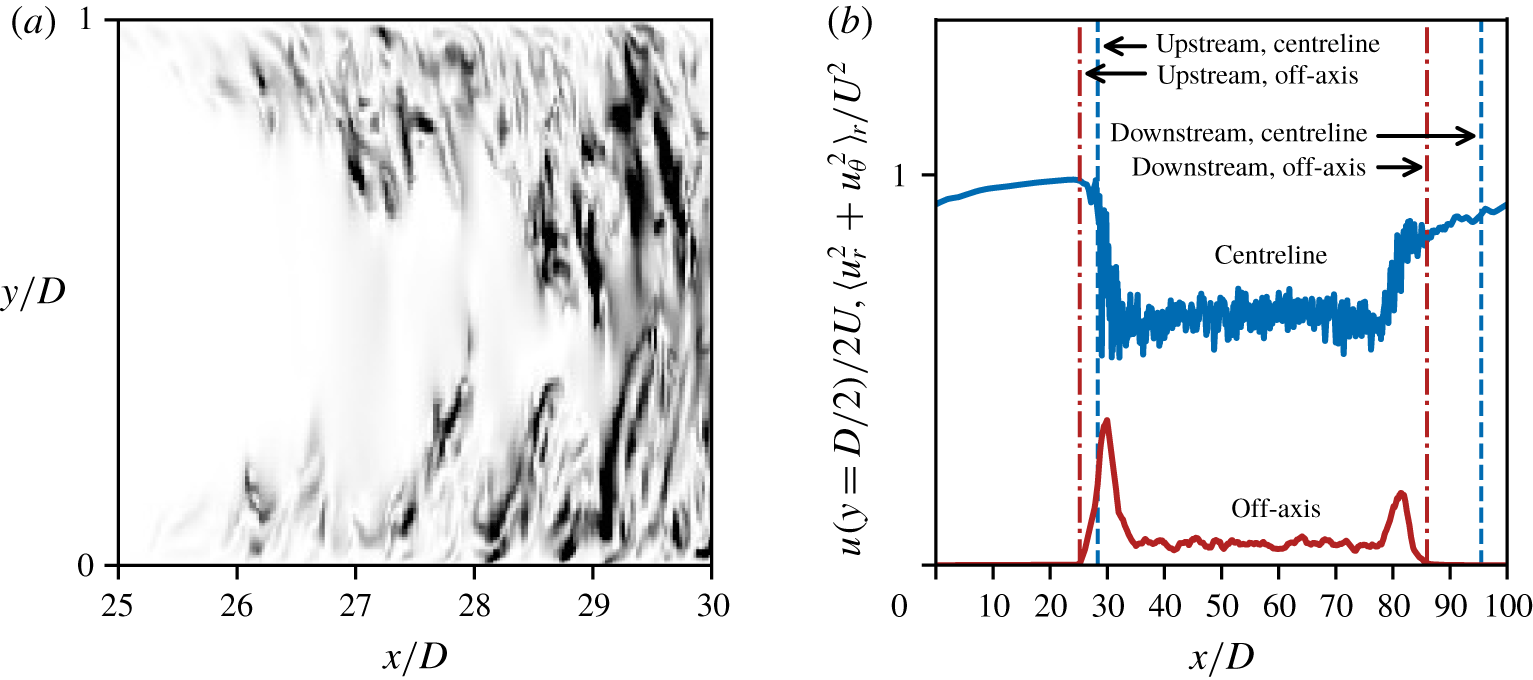
An immediate problem is how to objectively identify an interface, which itself has a profile (figure 3a). We consider two methods for identifying the interface and illustrate them using DNS data for transitional flow with slugs (figure 3b). For the first method, like WC, we threshold the centreline axial velocity. We identify the interface position as the point where this velocity drops 10 % below its laminar value. (WC did not specify the threshold they employed.) For the second method, we threshold the off-axis kinetic energy (per unit mass) averaged over the radius:  $\langle u_{r}^{2}+u_{\unicode[STIX]{x1D703}}^{2}\rangle _{r}$. (To denote the velocity components of time-averaged velocity and r.m.s. of velocity fluctuations, we use no subscript for the axial component, but for the radial and azimuthal components, we use the subscripts $r$ and $\unicode[STIX]{x1D703}$, respectively.) We identify the interface position as the point where this energy exceeds $5\times 10^{-4}U^{2}$. Note that changing this threshold value by an order of magnitude shifts the position of the interface by only ${\sim}1D$.
The two methods give a similar position for the sharp upstream interface, differing by  ${\sim}3D$, but the difference can be much larger for the gradual downstream interface, differing by ${\sim}10D$ (figure 3). Our purpose is not to judge which method is superior, but to point out the potential for ambiguity when discussing the interface. Following the currently standard approach, here we use the second method; for the DNS, we threshold $\langle u_{r}^{2}+u_{\unicode[STIX]{x1D703}}^{2}\rangle _{r}$, and for the experiments, we threshold $\langle u_{r}^{2}\rangle _{r}$.
How the flow in a slug develops near the upstream interface. Using DNS of transitional flow with slugs at  $Re=8000$, in the panels top to bottom, we plot unitless off-axis kinetic energy (which we use to identify the interface); MVPs; r.m.s. profiles; and total stress profiles. Note that the abscissa, $\unicode[STIX]{x0394}x/D$, the distance from the upstream interface, is plotted on a non-uniform scale, where the region near the interface is stretched. ( $\unicode[STIX]{x0394}x/D>0$ signals the interior of the slug.) We plot the diagnostic profiles (black curves) at a few representative $\unicode[STIX]{x0394}x/D$; for comparison, we also plot the attendant interior profiles (grey curves), which, by construction, are independent of $\unicode[STIX]{x0394}x/D$. For $\unicode[STIX]{x0394}x/D\gtrsim 10$, the diagnostic profiles (black curves) do not change with $\unicode[STIX]{x0394}x/D$ and overlap with the interior profiles (grey curves), signalling fully developed flow. (The MVPs become independent of $\unicode[STIX]{x0394}x/D$ sooner – for $\unicode[STIX]{x0394}x/D\gtrsim 6$.)

How the flow in a slug develops near the downstream interface. This figure is the downstream analogue of figure 4. Note that  $\unicode[STIX]{x0394}x/D$ increases opposite to the flow direction.
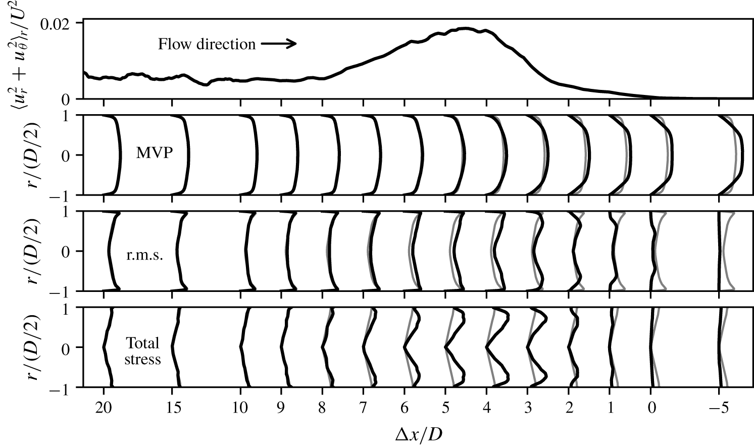
We now consider how the flow in a slug develops near the interfaces. To illustrate, in figures 4 and 5, using DNS data for transitional flow with slugs, we plot MVPs, r.m.s. profiles and total stress profiles ( $\unicode[STIX]{x1D70F}_{tot}$ profiles; see § 4.3) at a few representative axial distances, $\unicode[STIX]{x0394}x$, from the upstream and downstream interfaces, respectively. To obtain a profile at a fixed $\unicode[STIX]{x0394}x/D$, we compute the profile at that $\unicode[STIX]{x0394}x/D$ from each velocity field in an ensemble and then average those profiles over all the fields in the ensemble (see § 2). For ease of comparing the profiles at different $\unicode[STIX]{x0394}x/D$, we also plot an ‘interior profile’, which we compute by averaging the profiles over the entire axial extent of the slug save for the region $30D$ from both interfaces. (If the flow is fully developed, the interior profile and the profile at a fixed $\unicode[STIX]{x0394}x/D$ are indistinguishable.) As expected, the profiles close to the interfaces depend on $\unicode[STIX]{x0394}x/D$. However, in the interior of the slug, for $\unicode[STIX]{x0394}x/D\gtrsim 10$ from either interface, the profiles become independent of $\unicode[STIX]{x0394}x/D$ and collapse onto the attendant interior profile – the flow becomes fully developed.
WC measured the diagnostic profiles at  $\unicode[STIX]{x0394}x/D=20$. Even though this location satisfies the requirement for fully developed flow discussed above, recall that identifying the location of an interface itself can entail an ambiguity of ${\sim}10D$. Although with the information provided in WC we cannot objectively evaluate whether or not WC’s profiles are fully developed, WC’s choice of $\unicode[STIX]{x0394}x/D=20$ might have been too close to the interface, as the authors themselves suggest. But, if that is true, it follows that their data cannot be used to draw conclusions about the nature of slug flow. There is also an additional consideration: the role of $Re$, which we discuss next.
Testing the role of  $Re$ on flow development. Using DNS of transitional flow with slugs at $Re=3000$ and $8000$, we plot the relative difference (at a fixed $y/D$) for the following profiles versus $\unicode[STIX]{x0394}x/D$: (a) MVPs, (b) r.m.s. profiles and (c) total stress profiles. In computing a profile at a fixed $\unicode[STIX]{x0394}x/D$, we average the corresponding profiles at a distance $\unicode[STIX]{x0394}x/D\pm 1$ from both interfaces. We denote the interior profiles with the subscript ‘ $\infty$’. The vertical bars represent statistical error bars. The errors stem from the profiles at a fixed $\unicode[STIX]{x0394}x/D$; the statistical errors in the interior profile, by comparison, are negligible. For MVPs and r.m.s. profiles, we show $y/D=1/2$ and for total stress profiles, $y/D=1/4$; the results for other $y/D$ are comparable. For $\unicode[STIX]{x0394}x/D\gtrsim 15$, the relative difference in the MVPs is ${\lesssim}0.01$ and in the r.m.s. profiles and total stress profiles is ${\lesssim}0.1$.

In figure 6, we show the results from a quantitative analysis of how the profiles develop with  $\unicode[STIX]{x0394}x/D$ using DNS data at $Re=3000$ and $8000$, the lowest and highest $Re$, respectively, in our study. We consider profiles at a distance $\unicode[STIX]{x0394}x/D$ from both interfaces and take their average. Our quantitative measure is the relative difference, at a fixed $y/D$, between the value of a profile at $\unicode[STIX]{x0394}x/D$ compared with the attendant interior profile. By comparing the decay of the relative differences for the different diagnostics with $\unicode[STIX]{x0394}x/D$ at the two $Re$, we find that the distance needed for the flow to become fully developed increases with $Re$. This suggests that WC’s high- $Re$ data must be interpreted with caution.
In our study, the flow at  $Re=8000$ corresponds to the largest $\unicode[STIX]{x0394}x/D$ needed for the flow to be fully developed. From the profiles in figures 4 and 5, we have inferred that the flow is fully developed for $\unicode[STIX]{x0394}x/D\gtrsim 10$. From figure 6, we can ascribe quantitative values to the flow development. At $\unicode[STIX]{x0394}x/D=10$, the relative difference is ${\lesssim}0.03$ for the MVPs and ${\lesssim}0.3$ for the r.m.s. profiles and total stress profiles; at $\unicode[STIX]{x0394}x/D=15$, these values are, respectively, ${\lesssim}0.01$ and ${\lesssim}0.1$. By $\unicode[STIX]{x0394}x/D=30$, the lower limit we have chosen to compute the interior profiles, the relative differences are of the order of the statistical error.
Having demonstrated that the flow in a slug’s interior is fully developed, we can now proceed to meaningfully compare the diagnostic profiles for slug flow with those for fully turbulent flow. In the analysis henceforth, we identify the interior profiles as the diagnostic profiles for slug flow.
4 Diagnostic profiles
4.1 MVPs
The MVP,  $u(y)$, was the first measure used by WC as evidence for the equivalence between slug flow and fully turbulent flow. It also provides the clearest example of pipe flow’s $Re$-dependence. The textbook manner in which to compare MVPs of fully turbulent pipe flow at different $Re$ is to collapse the MVPs using two classical scaling laws (Pope Reference Pope2001). Near the wall, the ‘law of the wall’ dictates that plots of $u^{+}\equiv u/u_{\unicode[STIX]{x1D70F}}$ versus $y^{+}\equiv yu_{\unicode[STIX]{x1D70F}}/\unicode[STIX]{x1D708}$ for different $Re$ collapse onto one envelope. Away from the wall, the ‘defect law’ dictates that plots of $u^{+}(y=D/2)-u^{+}$ versus $y/D$ for different $Re$ collapse onto one envelope. These envelopes correspond to the asymptotic limit $Re\rightarrow \infty$. At large but finite $Re$, the MVPs collapse onto the corresponding envelope for a region and systematically peel away from the envelope as a function of $Re$: the higher the $Re$, the longer the MVP collapses onto the envelope (figure 7). If MVPs from slug flow also manifest these features, we can infer that slug flow is fully turbulent.
Classical scaling laws of MVPs in fully turbulent flow: (a) the law of the wall and (b) the defect law. The MVPs are from our DNS (we discuss  $Re=3000$ flow in the manuscript; we compute $Re=16\,000$ flow using the same code) and from Wu & Moin (Reference Wu and Moin2008) ( $Re=5300$ and $44\,000$). The $Re\rightarrow \infty$ envelope is represented by a thick grey line. At high $Re$, the MVPs systematically peel off from the corresponding envelopes as a function of $Re$. But, at low $Re$, this picture of systematically peeling off breaks down.
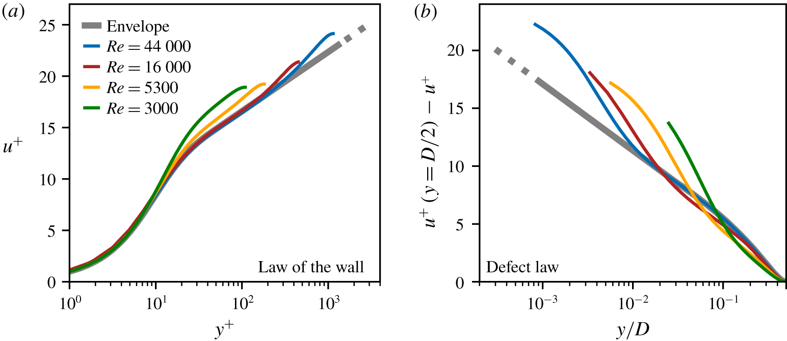
But – and this is a crucial point – at low  $Re$ this picture breaks down (figure 7). The systematic peeling away abruptly changes. The MVPs no longer collapse onto the envelopes, save for a small region (e.g. $y^{+}\lesssim 10$ in figure 7a). This breakdown of the collapse appears to occur at different $Re$ for the two scaling laws, with the law of the wall failing for $Re\lesssim 10\,000$, and the defect law failing for $Re\lesssim 44\,000$ (Patel & Head Reference Patel and Head1969; Wu & Moin Reference Wu and Moin2008). More important, because the breakdown corresponds to the range of $Re$ that is typical of transitional pipe flow (Mullin Reference Mullin2011), we can no longer use the envelopes to determine if the slug flow MVPs are fully turbulent. These circumstances necessitate a different approach.
Our approach is predicated on a key attribute of pipe flow we noted earlier: at any  $Re\gtrsim 2700$, the flow exists as one of two states, transitional with slugs or fully turbulent. We will consider different $Re$ separately, and for each $Re$, we will compare slug flow and fully turbulent flow as a pair, testing whether their MVPs as well as other diagnostic profiles are identical. (Comparing slug flow with fully turbulent flow at the same $Re$ is equivalent to comparing them at the same friction Reynolds number, $Re_{\unicode[STIX]{x1D70F}}\equiv u_{\unicode[STIX]{x1D70F}}D/\unicode[STIX]{x1D708}$; this is because the friction in both flows obeys the Blasius law (Cerbus et al. Reference Cerbus, Liu, Gioia and Chakraborty2018).) This approach, which forms the leitmotif of our analysis, allows us to account for the $Re$-dependence of the diagnostics without having to explicitly invoke a theoretical framework that underlies the $Re$-dependence. (We mention in passing that this approach cannot be used for puffs and for slugs at $Re\lesssim 2700$, since fully turbulent flow is not possible at the same $Re$.)
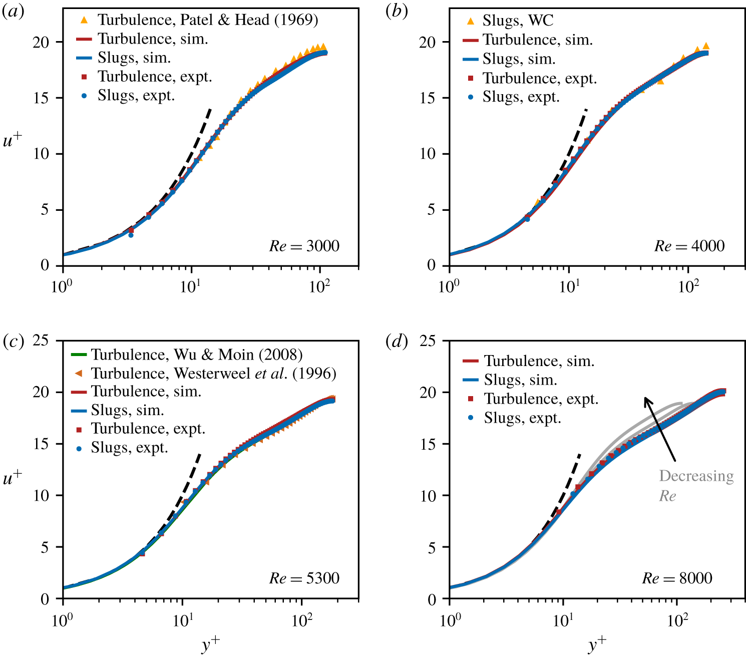
Comparing slug flow and fully turbulent flow using MVPs. We plot MVPs from our experiments (expt.), DNS (sim.) and the literature (Patel & Head Reference Patel and Head1969; WC; Westerweel et al. Reference Westerweel, Draad, Van der Hoeven and Van Oord1996; Wu & Moin Reference Wu and Moin2008) for  $Re=3000$ (a), $4000$ (b), $5300$ (c) and $8000$ (d) in the law-of-the-wall coordinates. The dashed line shows the linear profile, $u^{+}=y^{+}$, for the viscous sublayer. In (d) we include the MVPs from DNS at lower $Re$ (fully turbulent flow) in grey to highlight the $Re$-dependence of the MVPs. The statistical errors in our data are comparable to the size of the symbols.
Before turning to our results, we first discuss the analysis of WC. They plotted the MVPs (for flows at different  $Re$) as $u/u(y=D/2)$ versus $y/D$ (figure 2a). WC’s analysis is predicated on the expectation that the MVPs collapse in these unitless coordinates. This expectation is equivalent to stating that
 $$\begin{eqnarray}\displaystyle \frac{u}{u(y=D/2)}=f_{1}(y/D), & & \displaystyle\end{eqnarray}$$
 where  $f_{1}$ is a function that depends only on $y/D$. This relation, however, is contrary to the classical scaling laws. Consider, e.g. the defect law. The defect law can be expressed as $u-u(y=D/2)=u_{\unicode[STIX]{x1D70F}}f_{2}(y/D)$, where $f_{2}$ is a function that depends only on $y/D$. That is
 $$\begin{eqnarray}\displaystyle \frac{u}{u(y=D/2)}=1+\frac{u_{\unicode[STIX]{x1D70F}}}{u(y=D/2)}f_{2}(y/D), & & \displaystyle\end{eqnarray}$$
 which contradicts (4.1) because  $u_{\unicode[STIX]{x1D70F}}/u(y=D/2)$ depends on $Re$. Thus, even if we ignore the limitations of the classical scaling laws discussed above, the very basis of WC’s analysis of the MVPs is erroneous. Now, considering the fact that no scaling laws are known for the typical $Re$ of interest in slug flow, we must adopt the approach proposed above. But we cannot use this approach to analyse WC’s data because their slug flow and fully turbulent flow correspond to different $Re$.
$Re$.
To test for correspondence between slug flow and fully turbulent flow, using experiments and DNS, we generate two flows at the same  $Re$: transitional flow with slugs and fully turbulent flow. (These data provide the basis for our analysis of all the diagnostic profiles.) In figure 8(a–d), we plot the corresponding MVPs. (We plot the MVPs as $u^{+}$ versus $y^{+}$, although this is of no significance since the $Re$ is the same in each panel.) In all cases, over the entire cross-section of the pipe, the MVPs for slug flow and fully turbulent flow at the same $Re$ are indistinguishable. Thus, by the diagnostic of the MVP, slug flow is but fully turbulent flow. Our conclusion echoes that of WC, though, with the crucial caveat that slug flow and fully turbulent flow must be compared at the same $Re$.
$Re$.
4.2 The r.m.s. profiles
The r.m.s. profiles have not garnered as much attention as the MVPs, and are also comparatively less understood. It is unclear if these profiles have an analogue of the MVP scaling laws we discussed earlier. Indeed, recent experiments have demonstrated that, even at very high  $Re$, no unitless coordinates are known in which the r.m.s. profiles for different $Re$ would collapse onto an envelope (Willert et al. Reference Willert, Soria, Stanislas, Klinner, Amili, Eisfelder, Cuvier, Bellani, Fiorini and Talamelli2017).
Comparing slug flow and fully turbulent flow using r.m.s. profiles. We plot r.m.s. profiles from our experiments (expt.), DNS (sim.) and the literature (WC; Westerweel et al. Reference Westerweel, Draad, Van der Hoeven and Van Oord1996; Wu & Moin Reference Wu and Moin2008) for  $Re=3000$ (a), $4000$ (b), $5300$ (c) and $8000$ (d). For our experiments, we report $u^{^{\prime }+}$ and $u_{r}^{^{\prime }+}$; for our DNS, we report $u^{^{\prime }+}$, $u_{r}^{^{\prime }+}$ and $u_{\unicode[STIX]{x1D703}}^{^{\prime }+}$. In (d) we include the $u^{^{\prime }+}$ curves from DNS at lower $Re$ (fully turbulent flow) in grey to highlight the $Re$-dependence of the r.m.s. profiles (also see figure 10). The statistical errors in our data are comparable to the size of the symbols.

Consider WC’s analysis. They compared r.m.s. profiles ( $u^{^{\prime }+}$, $u_{r}^{^{\prime }+}$ and $u_{\unicode[STIX]{x1D703}}^{^{\prime }+}$ versus $y/D$) for slug flow and fully turbulent flow at different $Re$, just as they did with the MVPs. (In figure 2b, we show WC’s $u^{^{\prime }+}$ profiles.) And, just as was the case for the MVPs, there is no justification for these unitless profiles to collapse onto one envelope. In fact, empirical data for fully turbulent flow show that the unitless r.m.s. profiles do not collapse onto one envelope for any range of $Re$. Thus, here too, the very basis of WC’s analysis is erroneous.
The problem that no scaling laws are known to collapse r.m.s. profiles does not pose any difficulty for our approach. As with the MVPs, we compare the r.m.s. profiles of slug flow and fully turbulent flow at the same  $Re$ (figure 9). We find excellent agreement between slug flow and fully turbulent flow over the entire cross-section of the pipe. (We also compare the r.m.s. profiles from WC at $Re=4200$ with ours at $Re=4000$ and find them to be in poor agreement; see figure 9b.) Based on our analysis of r.m.s. profiles, we conclude that slug flow is identical to fully turbulent flow.
The  $Re$-dependence of the peak of the $u^{^{\prime }+}$ profile for fully turbulent flow. The data are from our DNS (discussed in the manuscript as well as other higher- $Re$ simulations we conducted using the same code), from DNS of Wu & Moin (Reference Wu and Moin2008) ( $Re=24\,000$ and $44\,000$) and from experiments of Willert et al. (Reference Willert, Soria, Stanislas, Klinner, Amili, Eisfelder, Cuvier, Bellani, Fiorini and Talamelli2017) ( $Re\geqslant 250\,000$). We plot (a) unitless positions of the peak, $y_{peak}/D$ and $y_{peak}^{+}$, versus $Re$ and (b) unitless magnitudes of the peak, $u_{peak}^{\prime }/U$ and $u_{peak}^{^{\prime }+}$, versus $Re$.
$Re$.

As an aside, we comment on the peak of the  $u^{^{\prime }+}$ profiles to highlight its rich $Re$-dependence. In figure 9(d), we superpose the $u^{^{\prime }+}$ profiles for fully turbulent flow at the different $Re$ of our study. (In light of the discussion above, the same analysis also holds for slug flow.) The $y/D$ position of the peak decreases with $Re$ and the magnitude of the peak stays roughly the same. For a clearer picture, we plot the peak position ( $y_{peak}$) and peak magnitude ( $u_{peak}^{\prime }$), using two unitless measures and over a broad range of $Re$, in figure 10. Note that whereas $y_{peak}/D$ decreases with $Re$,
$Re$,  $y_{peak}^{+}$ remains roughly constant over the whole range of $Re$ (figure 10a). The behaviour of $u_{peak}^{\prime }$ is more complex: $u_{peak}^{\prime }/U$ monotonically decreases with $Re$, but $u_{peak}^{^{\prime }+}$ is roughly constant at low $Re$ and increases with $Re$ for $Re\gtrsim 15\,000$ (figure 10b).
4.3 Total stress profiles
Last, we turn to the total (shear) stress profiles,  $\unicode[STIX]{x1D70F}_{tot}(y)$. In a fully developed flow (of which fully turbulent flow is a subset), the total stress profile obeys the exact relation for stress balance (Pope Reference Pope2001): $\unicode[STIX]{x1D70F}_{tot}^{+}\equiv \unicode[STIX]{x1D70F}_{\unicode[STIX]{x1D708}}^{+}+\unicode[STIX]{x1D70F}_{Re}^{+}=1-2y/D$, where $\unicode[STIX]{x1D70F}_{tot}^{+}$, the total stress, is the sum of $\unicode[STIX]{x1D70F}_{\unicode[STIX]{x1D708}}^{+}$, the viscous stress, and $\unicode[STIX]{x1D70F}_{Re}^{+}$, the Reynolds stress; all stresses are normalized by $\unicode[STIX]{x1D70F}_{w}$, the wall stress. Unlike the diagnostics of MVP and r.m.s. profile, the $\unicode[STIX]{x1D70F}_{tot}^{+}$ profile is independent of $Re$, although the $\unicode[STIX]{x1D70F}_{\unicode[STIX]{x1D708}}^{+}$ and $\unicode[STIX]{x1D70F}_{Re}^{+}$ profiles themselves are $Re$-dependent. The $\unicode[STIX]{x1D70F}_{tot}^{+}$ profile provides an exact quantitative test of the fully developed nature of slug flows, complementing our discussion of § 3.
Representative Reynolds stress profiles from WC,  $\unicode[STIX]{x1D70F}_{Re}^{+}$ versus $y/D$ (cf. figure 20 in WC). Here, we show results for the profiles near the upstream interface; the profiles near the downstream interface are similar. The dashed line represents the stress-balance relation, $\unicode[STIX]{x1D70F}_{Re}^{+}\approx 1-2y/D$.

Comparing slug flow and fully turbulent flow using total stress profiles. We plot  $\unicode[STIX]{x1D70F}_{tot}^{+}$ profiles from our experiments (expt.), DNS (sim.) and the literature (WC; Westerweel et al. (Reference Westerweel, Draad, Van der Hoeven and Van Oord1996), Wu & Moin (Reference Wu and Moin2008)) for $Re=3000$ (a), $4000$ (b), $5300$ (c) and $8000$ (d). The dashed line in each plot represents the stress-balance relation, $\unicode[STIX]{x1D70F}_{tot}^{+}=1-2y/D$. In (b), we also show WC’s $\unicode[STIX]{x1D70F}_{tot}^{+}$ profile for slug flow. To compute that profile, we added WC’s $\unicode[STIX]{x1D70F}_{Re}^{+}$ profile at $Re=4200$ and $\unicode[STIX]{x1D70F}_{\unicode[STIX]{x1D708}}^{+}$ profile at $Re=4000$. (They did not report these profiles at the same $Re$.) The statistical errors in our data are comparable to the size of the symbols.

WC plotted  $\unicode[STIX]{x1D70F}_{Re}^{+}$ versus $y/D$ for slug flows and fully turbulent flow (figure 11). Note that although the $\unicode[STIX]{x1D70F}_{Re}^{+}$ profile depends on $Re$, at high $Re$ and away from the wall, $\unicode[STIX]{x1D70F}_{Re}^{+}\approx \unicode[STIX]{x1D70F}_{tot}^{+}$, so one can use the $\unicode[STIX]{x1D70F}_{Re}^{+}$ profile as an $Re$-independent diagnostic. Thus, unlike their analysis of the MVPs and r.m.s. profiles, WC’s analysis of $\unicode[STIX]{x1D70F}_{Re}^{+}$ profiles (in the region away from the wall) does not suffer from improper accounting for the $Re$-dependence of the diagnostic profiles. The problem, however, is with the data themselves. Whereas WC’s $Re=50\,000$ fully turbulent flow profile conforms to the stress-balance relation, which corroborates the experimental accuracy, the $Re=19\,000$ and $Re=4200$ slug flow profiles undershoot and overshoot the said relation, respectively. This suggests that slug flow is not fully developed, thereby casting doubt on the very exercise of comparing it with fully turbulent flow.
We plot  $\unicode[STIX]{x1D70F}_{tot}^{+}$ versus $y/D$ for slug flows and fully turbulent flow (figure 12). Although this is an $Re$-independent diagnostic, for clarity we group the plots by the value of $Re$. In stark contrast to WC, our data show excellent agreement with the stress-balance relation for all values of $Re$. Based on our analysis of $\unicode[STIX]{x1D70F}_{tot}^{+}$ profiles, we conclude that slug flows are fully developed. This, coupled with the result that at the same $Re$ the $\unicode[STIX]{x1D70F}_{\unicode[STIX]{x1D708}}^{+}$ profiles for slug flows and fully turbulent flows are indistinguishable (cf. figure 8), implies that the corresponding $\unicode[STIX]{x1D70F}_{Re}^{+}$ profiles are indistinguishable as well.
5 Summary
Is slug flow identical to fully turbulent flow? Seeking a clear answer to this question has motivated this study.
It is widely thought that a clear answer was furnished by the pioneering study of WC, which concluded, ‘the structure of the flow in the interior of the slug is identical to that in a fully developed turbulent pipe flow’. By reanalysing the diagnostic profiles (MVPs, r.m.s. profiles and stress profiles) from WC, we have shown that this well-known conclusion cannot be substantiated based on their data.
We conducted experiments and simulations, paying careful attention to two aspects. First, we established that, for a slug, despite the inexorable march of its interfaces, away from the interfaces and inside the slug, the flow diagnostics are independent of the axial location – that is, the slug flow is fully developed. Second, noting the  $Re$-dependence of the diagnostic profiles in fully turbulent flow, we compared slug flow with fully turbulent flow at the same value of $Re$. From our analysis we conclude that slug flow is indeed identical to fully turbulent flow with the crucial caveat that the two flows are compared at the same value of $Re$. Our re-examination of WC’s seminal work reveals a richer – and a more accurate – picture of the $Re$-dependence of transitional pipe flows.
Acknowledgements
This work was supported by the Okinawa Institute of Science and Technology (OIST) Graduate University. R.T.C. gratefully acknowledges the support of JSPS (KAKENHI 17K14594). We thank the Scientific Computing and Data Analysis section at OIST for computational support.


 Open access