


Introduction
L’analyse mathématique peut déduire des phénomènes généraux et simples l’expression des lois de la nature; mais l’application spéciale de ces lois à des effets très-composés exige une longue suite d’observations exactes.1 (Joseph Fourier, 1768–1830)
This quote by Joseph Fourier appeared first in the ‘discours préliminaire’ of the analytical theory of heat.Reference Fourier2 With this sentence, Fourier expresses the need of an inductive approach to complex physical phenomena at the macroscopic scale. He repeated it at least once, to conclude his mémoire sur les températures du globe terrestre et des espaces planétaires,Reference Fourier3 in which Fourier formulates what is known today as the ‘greenhouse effect’. Fourier confesses that ‘the question of Earth’s temperature is one of the most important and difficult of all the Natural Philosophy’Reference Fourier3 and solving it was one central motivation for the theory of heat. Clearly, Fourier had fully perceived the complex character of the climate system. How, two centuries later, do we cope with climate’s complexity? Which mathematical analysis is the most appropriate to get the best out of observations? With this paper, we wish to convince the reader that the most complex model is not necessarily the most useful. Predicting and understanding the climate system requires a consistency between the level of complexity of observations, model prediction and what one wants to predict. Choosing the right model is thus also a question of information theory.
The case will be illustrated through a polemic currently taking place in the circle of Quaternary climate scientists. As we shall see in more detail, the climate history of the past few million years is characterised by repeated transitions between ‘cold’ (glacial) and warm (interglacial) climates. The first modern men were hunting mammoth during the last glacial era. This era culminated around 19,000 years agoReference Lambeck, Yokoyama, Johnston and Purcell4 and then declined rapidly. By 9000 years ago, the climate was close to the modern one. The current interglacial, called the Holocene, has lasted about the same time as previous interglacials. The polemic is about when it is supposed give way to a new glacial inception, keeping aside human activities that have most probably perturbed natural cycles.
On the one side, Bill Ruddiman, Professor of Environmental Sciences, carefully inspected and compared palaeo-environmental information about the different interglacial periods. This comparison let him to conclude that glacial inception is largely overdue.Reference Ruddiman5, Reference Ruddiman6 According to him, the Holocene was not supposed to be that long, but the natural glacial inception process was stopped by an anthropogenic perturbation that began as early as 6000 years ago (rice plantations and land management by antique civilisations). On the other side, Professor André Berger and colleagues developed a mathematical model of the climate system, rated today as a ‘model of intermediate complexity’Reference Gallée, van Ypersele, Fichefet, Tricot and Berger7, Reference Gallée, van Ypersele, Fichefet, Marsiat, Tricot and Berger8 including 15,000 lines of FORTRAN code to solve the dynamics of the atmosphere and ice sheets on a spatial grid of 19 × 5 elements, with a reasonably extensive treatment of the shortwave and longwave radiative transfers in the atmosphere. Simulations with this model led Berger and Loutre to conclude that glacial inception is not due before 50,000 years as long as the CO2 atmospheric concentration stays above 220 ppmv.Reference Berger and Loutre9 Who is right? Both (Crucifix and Berger argued that the two statements are not strictly incompatibleReference Crucifix and Berger10)? Neither? Both Ruddiman and Berger judge that it is possible to predict climate thousands of years ahead, but is this a realistic expectation? Michael GhilReference Ghil11 wondered ‘what can we predict beyond one week, for how long and by what methods?’ This is the fundamental motivation behind the present article.
Steps towards a dynamical model of palaeoclimates
An inductive approach to complex system modelling
A system as complex as climate is organised at different levels: clouds, cloud systems, synoptic waves, planetary waves, pluri-annual oscillations such as El-Niño, glacial–interglacial cycles, and so on. These patterns constitute information that is susceptible to being modelled, understood and predicted.
Schematically, spatio-temporal structures are created by instabilities (necessarily fed by some source of energy), and destroyed by relaxation processes (return to equilibrium). The resulting stationary patterns are a balance between both. A typical laboratory example is the Bénard Cells. In the atmosphere, local hydrodynamical instabilities result in planetary waves, such as the ones responsible for dominant north-westerly winds in Canada and south-westerly winds in Europe.
In order to predict the macroscopic properties of atmospheric waves, it is more useful to consider the conditions under which the instability may develop (the thermal gradient, the jet stream and the position of the Rockies) than the time and position of the hypothetic butterfly that triggered the initial instability. The latter information is irrelevant in the sense that it does not help us to provide a reliable prediction. (Some philosophers say here that the cause of the baroclinic wave is then the jet stream and not the butterflyReference Cartwright12 because if I wanted to change the shape of the wave I would act on the jet stream, not on the butterfly).
Our understanding of a complex system may therefore be rated by (1) our capacity to formulate powerful predictive models linking causes to effects at the macroscopic scale; and (2) establishing logical connections between different scales of description, from the microscopic one to the coarsest-grained macroscopic.
Returning to the Bénard cell example, task (1) consists of formulating the hydrodynamical model that explains the Bénard cell pattern through the growth of the most unstable wave, given the boundary conditions, and task (2) is to infer water viscosity from its molecular structure.
We have just seen that macroscopic patterns depend on the parameters that control the growth of instabilities. Unfortunately, only in relatively idealised and simple cases is it possible to correctly predict macroscopic patterns from the microscopic scale. In most natural cases, the mechanisms of instability growth are so numerous and intricate that the resulting effects cannot possibly be predicted without appropriate observations. Namely, Saltzman repeatedly insistedReference Saltzman, Hansen and Maasch13, Reference Saltzman14 on the fact that neither current observations nor modelling of the present state of the atmosphere can possibly inform us of the ice-sheet mass balance with sufficient accuracy to predict the evolution of ice sheets at the timescale of several thousands of years. We need to look at palaeoclimate history to get this information.
Climate models should therefore be developed according to an inductive process: physical arguments provide a prior on the system dynamics and parameters, and observations lead us to update the parameters of this model. If the prior model turns out to be unsatisfactory, new physical considerations are needed to refine the model. This inductive approach never allows us to affirm that one model is correct, but it is expected gradually to lead us to models that have good explanatory power while being at the same time parsimonious and physically sound.
In The Logic of Science JaynesReference Jaynes15 provides a number of elements of statistical decision theory needed to proceed safely. The foundations date back to the works of Bayes, Bernouilli and Laplace (who formalised the principle of non-informative prior), and then Gibbs and Boltzman, according to which the second principle of thermodynamics is a logical consequence of the fact that one instance of a macroscopic variable may be realised by many different microscopic configurations. What have been termed causes here, become constraints in the inductive paradigm – one example is the conservation of energy. Constraints put conditions on our predictions, and our job is to identify and understand which constrains are needed to provide good predictions.Reference Fourier2 For example, it is observed that the atmospheric circulation of several planets of the solar system, including the Earth, is close to a regime of maximum entropy production under the single constraint of energy balance, given surface albedo.Reference Lorenz, Lumine, Withers and McKay16 This observation suggests to us that the rotation rate and atmospheric composition do not effectively constrain the magnitude of the poleward heat transport in these planets (see also Ref. Reference Ozawa, Ohmura, Lorenz and Pujol17). DewerReference Dewar18 proposed a formal derivation of the maximum entropy production principle based on Jayne’s MaxENT formalism,Reference Jaynes19 but objections have been raised.Reference Grinstein and Linsker20
Empirical evidence about the quaternary
Building a robust theory of glacial–interglacial cycles requires a profound knowledge of the Quaternary. This section has no more ambition than to provide a short glimpse at the vast amount of knowledge that scientists have accumulated on that period before we tackle Ruddiman’s hypothesis.
The natural archives. By the 1920s, geomorphologists were able to interpret correctly the glacial moraines and alluvial terraces as the leftovers of previous glacial inceptions. Penk and BrücknerReference Penck and Brückner21 (cited by BergerReference Berger22) recognised four previous glacial epochs, named the Günz, Mindel, Riss and Würm. The wealth of data on the Quaternary environments that has since been collected and analysed by field scientists can be appreciated from the impressive four-volume Encyclopedia of Quaternary Sciences recently edited by Elias.Reference Elias23 Analysis of and interpreting palaeoenvironmental data involve a huge variety of scientific disciplines, including geochemistry, vulcanology, palaeobiology, nuclear physics, stratigraphy, sedimentology, glacial geology and ice-stream modelling.
Only a schematic overview of this rich and intense field of scientific activity could possibly be given here. The reader will find most of the relevant references in the Encyclopedia of Quaternary Sciences, and only a few historical ones are provided here.
Stable isotopes constitute one important class of natural archives. It is indeed known, since the works of Urey,Reference Urey24 BuchananReference Buchanan, Nakao and Edwards25 and DansgaardReference Dansgaard26 that physical and chemical transformations involved in the cycles of water and carbon fractionate the isotopic composition of these elements. To take but a few examples, ice-sheet water is depleted in oxygen-18 and deuterium compared with sea water; clouds formed at low temperatures are more depleted in oxygen-18 and deuterium than clouds formed at higher temperatures; organic matter is depleted in 13C, such that inorganic carbon present in biologically active seas and soils is enriched in 13C. 15N is another useful stable palaeo-environmental indicator sensitive to the biological activity of soils. The isotopic compositions of water and biogenic carbon are extracted deep-sea sediments, ice and air trapped in ice bubbles, palaeosols, lake-sediments and stalagmites. One of the first continuous deep-sea records of glacial-interglacial cycles was published by Cesare Emiliani.Reference Emiliani27
Radioactive tracers are used to estimate the age of the record and rate of ocean water renewal. At the timescale of the Quaternary, useful mother-daughter pairs are 230Th/238,234U (dating carbonates), and 40K/40Ar in potassium-bearing minerals. The ratio 230Th/231Pa is a useful indicator of ocean circulation rates.
The chemical composition of fossils is also indicative of past environmental conditions. In the ocean, cadmium, lithium, barium and zinc trapped in the calcite shells of foraminifera indicate the amount of nutrients at the time of calcite formation, while the foraminifera content in magnesium and strontium are empirically correlated to water-temperature.
Glaciologists have also developed ambitious programmes to analyse the composition of air (oxygen, nitrogen, plus trace gases such as methane, carbon-dioxide and nitrogen oxide, argon and xenon) trapped in ice accumulating on ice sheets, of which the European Project for Ice Core in Antarctica is a particularly spectacular achievement.Reference Jouzel, Masson-Delmotte, Cattani, Dreyfus, Falourd and Hoffman28 It was demonstrated that the central plateaus of Antarctica offer a sufficiently stable environment to reliably preserve air’s chemical composition over several hundreds of thousands of years. The chemical composition of water is sensitive to atmospheric circulation patterns and sea-ice area.
Additional sources of information are obtained from a variety of marine and continental sources. Plant and animal fossils (including pollens) trapped in lakes, peat-bogs, palaeosols and marine sediments provide precious indications on the palaeoenvironmental conditions that conditioned their growth. Their presence (quantified by statistical counts) or absence may be interpreted quantitatively to produce palaeoclimatic maps.29 Preservation indicators of ocean calcite fossils are used to reconstruct the history of ocean alkalinity. Palaeosols and wind-blown sediments (loess) provide precious indications on past aridity at low-latitudes. The loess grain-size distribution is also sensitive to atmospheric circulation patterns. Geomorphological elements remain a premium source of information about the configuration of past ice sheets, which is complemented by datable evidence (typically coral fossils) on sea-level.
The structure of Quaternary climate changes. It is straightforward to appreciate which fraction of the information available in a climate record is relevant to understanding climate dynamics at the global scale. For example, minor shifts in oceanic currents may have sensible effects on the local isotopic composition of water with, however, no serious consequence for glacial–interglacial cycle dynamics. One strategy is to collect samples from many areas of the world and average them out according to a process called ‘stacking’. One of the first ‘stacks’, still used today, was published by John Imbrie and colleaguesReference Imbrie, Hays, Martinson, McIntyre, Mix and Morley30 in the framework of the Mapping Spectral Variability in Global Climate Project. It is usually referred to as the SPECMAP stack. Here, we concentrate on the more recent compilation provided by Lisiecki and Raymo,Reference Lisiecki and Raymo31 called LR04. The stack was obtained by superimposing 57 records of the oxygen-18 composition of benthic foraminifera shells. Benthic foraminifera live in the deep ocean and therefore record the isotopic composition of deep water (an indicator of past ice volume). However, there is an additional fractionation associated to the calcification process, which is proportional to water temperature. The isotopic composition of calcite oxygen is reported by a value, named δ18Oc, giving the relative enrichment of oxygen-18 versus oxygen-16 compared with an international standard. High δ18O indicates either low continental ice volume and/or high water-temperature.
Visual inspection of the LR04 stack (Figure 1) nicely shows the gradual transition from the Pliocene – warm and fairly stable – to the spectacular oscillations of the late Pleistocene. The globally averaged temperature at the early Pliocene was about 5°C higher than today (Ref. Reference Raymo, Grant, Horowitz and Rau32 and references therein); and the globally averaged temperature at the last glacial maximum (20,000 years ago) was roughly 5°C lower. Our central research is to characterise these oscillations, understand their origin and qualify their predictability.
The LR04 benthic δ18O stack constructed by the graphic correlation of 57 globally distributed benthic δ18O records.Reference Lisiecki and Raymo31 Note that the full stack goes back in time to −5.2 Myr (1 Myr = 1 million years). The signal is the combination of global ice volume (low δ18O corresponding to low ice volume) and water temperature (low δ18O corresponding to high temperature). The Y-axis is reversed as standard practice to get ‘cold’ climates down. Data downloaded from http://www.lorraine-lisiecki.com

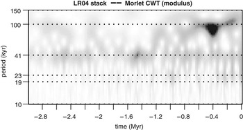
The Morlet Continuous wavelet transform provides us with a first outlook on the backbone of these oscillations (Figure 2). The LR04 record is dominated most of the time by a 40,000 year signal, until roughly 900,000 years ago, after which the 40,000 year signal is still present but topped by longer cycles. At the very least, this picture should convince us that LR04 contains structured information susceptible of being modelled and possibly predicted.
Modulus of the continuous Morlet Transform of the LR04 stack according to the algorithm given in Torrence and CompoReference Torrence and Compo33 using ω 0 = 5.4. R routine adapted by J. L. Melice and the author from the original code supplied by S. Mallat.Reference Mallat34 The wavelet transform shows the presence of quasi-periodic signals (shades) around periods of 41 kyr (1 kyr = 1000 years) and 1000 kyr
How many differential equations will be needed? There will be no clear-cut answer to that question. Time-series extracted from complex systems are sometimes characterised by their correlation dimension, which is an estimator for the fractal dimension of the corresponding attractor.Reference Grassberger and Procaccia35 The first estimates for the Pleistocene were provided by Nicolis and NicolisReference Nicolis and Nicolis36 (d = 3.4) and Maasch et al.Reference Maasch37 (4 < d < 6). For this article we calculated correlation dimension estimates for the LR04 stack (d = 1.54) and the HW04 stackReference Huybers and Wunsch38 (d = 3.56). HW04 is similar to LR04 but it is based on different records and dating assumptions. Several authors, including Grassberger himselfReference Grassberger39–Reference Vautard and Ghil41 have discouraged the use of correlation dimension estimates for the ‘noisy and short’ time series typical of the Quaternary because they are overly sensitive to sampling and record length. They are therefore unreliable.
In response to this problem, Ghil and colleaguesReference Vautard and Ghil41, Reference Yiou, Ghil, Jouzel, Paillard and Vautard42 promoted single-spectrum analysis, in which a time series is linearly decomposed into a number of prominent modes (which need not be harmonic), plus a number of small-amplitude modes. Assuming that the two groups are indeed separated by an amplitude gap, the first group provides the low-order backbone of the signal dynamics while the second group is interpreted as stochastic noise. Single spectrum analysis was applied with a certain success to various sediment and ice-core records of the few last-glacial interglacial cyclesReference Yiou, Ghil, Jouzel, Paillard and Vautard42 and have, in general, confirmed that the backbone of climate oscillations may be captured as a linear combination of a small number of amplitude and/or frequency-modulated oscillations. Single-spectrum analysis of the last million years of LR04 (Figure 3) confirms this statement.
Single Spectrum Analysis (SSA) of the LR04 and HW04 benthic stacks. Displayed are the eigenvalues of the lagged-covariance matrix of rank M = 100 as given by Ref. Reference Ghil, Allen, Dettinger, Ide, Kondrashov and Mann43, equation (6). The records were cubic-spline interpolated (Δt = 1 kyr) and only the most recent 900 kyr were kept. The SSA decomposition of LR04 is very typical: it shows three oscillators (recognisable as pairs of eigenvectors), then about four modes that are generally interpreted as harmonics of the dominant ones, and finally a number of modes typically interpreted as stochastic background. The HW04 stack contrasts with LR04 because the dominant modes are not so easily evidenced. HW04 uses less benthic records than LR04, but it also relies on more conservative dating assumptions and this probably resulted in blurring the quasi-periodic components of the signal. HW04 data were obtained from http://www.people.fas.harvard.edu/phuybers/

The Achilles Heel. Now the time has come to mention a particularly difficult and intricate issue: dating uncertainty in palaeoclimate records. No palaeoclimate record is dated with absolute confidence. Marine sediments are coarsely dated by identification of a number of reversals of the Earth’s magnetic field, which have been previously dated in rocks by radiometric means (Ref. Reference Raymo44 and references therein). Magnetic reversals are pretty rare (four of them over the last 3 million years) and their age is known with a precision no better than 5000 years. Local sedimentation rates may vary considerably between these time markers such that any individual event observed in any core taken in isolation is hard to date. Irregularities in the sedimentation rate blur and destroy information that might otherwise be shown by spectral analysis.
One strategy to contend this issue is to assume synchrony between oscillation patterns identified in different cores. Statistical tests may then be developed on the basis that dating errors of the different cores are independent. For example, HuybersReference Huybers45 considered the null-hypothesis that glacial–interglacial transitions (they are called terminations in the jargon of palaeoclimatologists) are independent on the phase of Earth’s obliquity. While this null-hypothesis could not be rejected on the basis of a single record, the combination of 14 cores allowed him to reject it with 99% confidence, proving once more the effect of the astronomical forcing on climate. The first tests of this kind were carried out by Hays et al.Reference Hays, Imbrie and Shackleton46 in a seminal paper. Note that in many cases the oscillation patterns recognised in different cores are so similar that it is hard to dispute the idea of somehow ‘matching them’, but it is remarkable that rigorous statistical tests assessing the significance of a correlation between two ill-dated palaeoclimate records are only being developed (Haam and Huybers, manuscript in preparation).
Another strategy is known as orbital tuning. The method consists of squeezing or stretching the time-axis of the record to match the evolution of one or a combination of orbital elements, possibly pre-filtered by a climate model.Reference Imbrie, Hays, Martinson, McIntyre, Mix and Morley30, Reference Hays, Imbrie and Shackleton46 The method undeniably engendered important and useful results (e.g. Ref. Reference Shackleton, Berger and Peltier47), but the astute reader has already perceived its potential perversity: orbital tuning injects a presumed link between orbital forcing and the record. Experienced investigators recognise that orbital tuning has somehow contaminated most of the dated palaeoclimate records available in public databases. This has increased the risk of tautological reasoning.
For example, compare the two SSA analyses shown in Figure 3. As mentioned, LR04 and HW04 are two stacks of the Pleistocene but LR04 contains more information. It is made of more records (57 instead of 21 in HW04) and it is astronomically tuned. We can see from the SSA analysis that LR04 presents more quasi-periodic structures than HW04 (recall that quasi-periodic modes are identified as pairs of eigenvalues with almost the same amplitude). Why is this the case? Is this because age errors in HW04 blurred the interesting information, or is it because this information has been artificially injected in LR04 by the tuning process? There is probably a bit of both (but note that HW04 displays a similar wavelet structure as LR04).
Leads and lags between CO2 and ice volume is another difficult problem, where risks posed by hidden dating assumptions and circular reasoning lie at every corner. Here is one typical illustration: Saltzman and Verbitsky have shown on several occasions (e.g. Ref. Reference Saltzman and Verbitsky48) a phase diagram showing the SPECMAP δ18O stack versus the first full ice-core records of CO2 available at that time.Reference Barnola, Raynaud, Korotkevich and Lorius49, Reference Jouzel, Barkov, Barnola, Bender, Chappellaz and Genthon50 It is reproduced here (Figure 4, left). The phase diagram clearly suggests that CO2 leads ice volume at the 100 kyr time scale. However, a detailed inspection of the original publications reveals that the SPECMAP record was astronomically tuned, and that the Vostok time-scale uses a conventional date of isotopic stage 5.4 of 110 kyr BP … by reference to SPECMAPReference Jouzel, Barkov, Barnola, Bender, Chappellaz and Genthon50! The hysteresis is therefore partly conditioned by arbitrary choices. In Figure 4 we further illustrate the fact that the shape of the hysteresis depends on the stack record itself. The situation today is that there is no clear consensus about the phase relationship between ice volume and CO2 at the glacial interglacial time scale (compare Refs Reference Kawamura, Parrenin, Lisiecki, Uemura, Vimeux and Severinghaus51–Reference Shackleton53). According to the quite careful analysis of Ref. Reference Ruddiman52, CO2 leads ice volume at the precession (20 kyr) period, but CO2 and ice volume are roughly synchronous at the obliquity (40 kyr) period. Current evidence about the latest termination is that a decrease in ice volume and the rise in CO2 were grossly simultaneous and began around 19,000 years ago.Reference Kawamura, Parrenin, Lisiecki, Uemura, Vimeux and Severinghaus51, Reference Yokoyama, Lambeck, de Deckker, Johnston and Fifield54
The concentration in CO2 measured in the Vostok ice core recordReference Petit, Jouzel, Raynaud, Barkov, Barnola and Basile55 over the last glacial-interglacial cycle is plotted versus two proxies of continental ice volume: (left) the planctonic δ18O stack by Imbrie et al. (1984); and (right) the benthic δ18O stack by Lisiecki and Raymo.Reference Lisiecki and Raymo31 Numbers are dates, expressed in kyr BP (before present). While the Imbrie stack suggests a hysteresis behaviour with CO2 leading ice-volume variations, the picture based on LR04 is not so obvious

Getting physical laws into the model
So far, we have learned that palaeoclimate oscillations are structured and that it is not unreasonable to attempt modelling them with a reduced order model forced by the astronomical variations of Earth’s orbit. What is the nature of the physical principles to be embedded in such a model, and how can they be formalised? The history of Quaternary modelling is particularly enlightening in this respect (the reader will find in Ref. Reference Berger22 an extensively documented review of Quaternary climates modelling up to the mid-1980s). After Joseph Adhémar (1797–1862) suggestedReference Adhémar56 that the cause of glaciations is the precession of the equinoxes, Joseph John Murphy and James Croll (1821–1890) argued about how precession may affect climate. Murphy maintained that cold summers (occurring when summer is at aphelion) favour glaciation,Reference Murphy57 while Croll considered that cold winters are critical.Reference Croll58
Croll’s book demonstrates a phenomenal encyclopaedic knowledge. His judgements are at places particularly far-sighted, but they are barely substantiated by the mathematical analysis Fourier was so much insistent about. The nature of his arguments is essentially phenomenological, if not, in places, frankly rhetorical.
Milutin Milankovitch (1879–1958) is then generally quoted as the person having most decisively crossed the step towards mathematical climatology. In a highly mathematical book that crowns a series of articles written between 1920 and 1941,Reference Milankovitch59 Milankovitch extends Fourier’s work to estimate the zonal distribution of the Earth’s temperature from incoming solar radiation. He also computes the effects of changes in precession, eccentricity and obliquity on incoming solar radiation at different latitudes to conclude, based on geological evidence, that summer insolation is indeed driving glacial–interglacial cycles.
Mathematical analysis is the process that allows Milankovitch to deduce the consequences of certain fundamental principles, such as the laws of Beer, Kirchhoff and Stefan, on global quantities such as Earth’s temperature. On the other hand, Milankovitch uses empirical macroscopic information, such as the present distribution of the snow-line altitude versus latitude, to estimate the effects of temperature changes on the snow cover. In today’s language, one may say that Milankovitch had accepted that some information cannot be immediately inferred from microscopic principles because they depend on the way the system as a whole has been dealing with its numerous and intricate constraints (Earth’s rotation, topography, air composition etc).
The marine-record study published by Hays, Imbrie and ShackletonReference Hays, Imbrie and Shackleton46 is often cited as the most indisputable proof of Milankovitch’s theory. Hays et al. identified three peaks in the spectral estimate of climate variations that precisely correspond to the periods of obliquity (40 kyr) and precession (23 kyr and 19 kyr) calculated analytically by André Berger (the supporting papers by Berger would only appear in the two following years;Reference Berger60–Reference Berger62 Hays et al. based themselves on a numerical spectrum estimate of the orbital time-series provided by VernekarReference Vernekar63).
However, sensu stricto, Milankovitch’s theory of ice ages was invalidated by evidence – already available in an article by Broecker and van DonckReference Broecker and van Donk64 – that the glacial cycle is 100,000 years long, with ice build up taking about 80,000 years and termination about 20,000 years.Reference Hays, Imbrie and Shackleton46, Reference Broecker and van Donk64 Neither the 100,000-year duration of ice ages, nor their saw-tooth-shape were predicted by Milankovitch. The bit Milankovitch’s theory is missing is the dynamical aspect of climate’s response. Glaciologist WeertmanReference Weertman65 consequently addressed the evolution of ice sheet size and volume by means of an ordinary differential equation, thereby opening the door to the use of dynamical system theory for understanding Quaternary oscillations.
In the meantime, general circulation models of the atmosphere and oceans running on supercomputers became widely available (cf. Ref. Reference Randall66 for a review), and used for palaeoclimate purposes.Reference Broccoli and Manabe67–Reference Mitchell69 The interest of these models is that they provide a consistent picture of the planetary dynamics of the atmosphere and the oceans. Just as Milankovitch applied Beer and Kirchoff’s laws to infer Earth’s temperature distribution, general circulation models allow us to deduce certain aspects of the global circulation from our knowledge of balance equations in each grid cell. However, these balance equations are uncertain and quantifying the consequences of these uncertainties at the Earth global scale is a very deep problem that only begins to be systematically addressed.Reference Allen, Stott, Mitchell, Schnur and Delworth70 While general circulation models are undeniably useful to constrain the immediate atmospheric response to changes in orbital parameters, they are far too uncertain to reliably estimate glacial accumulation rates with enough accuracy to predict the evolution of ice sheets over tens of thousands of years.Reference Saltzman, Hansen and Maasch13
In the following sections we will concentrate on a three-dimensional climate dynamical model written by Saltzman. This choice was guided by the ease of implementation as well as the impressive amount of supporting documentation.Reference Saltzman14 However, there were numerous alternatives to this choice. The reader is referred to the article by Imbrie et al.Reference Imbrie, Boyle, Clemens, Duffy, Howard and Kukla71 and pp. 264–265 of Saltzman’s bookReference Saltzman14 for an outlook with numerous references organised around the dynamical concepts proposed to explain glacial–interglacial cycles (linear models, with or without self-sustained oscillations, stochastic resonance, a model with large numbers of degrees of freedom).
The series of models published by Ghil and colleaguesReference Källén, Crafoord and Ghil72–Reference Le Treut and Ghil74 are among the ones having the richest dynamics. They present self-sustained oscillations with a relatively short period (6000 years). The effects of the orbital forcing are taken into account by means of a multiplicative coefficient in the ice mass balance equation. This causes non-linear resonance between the model dynamics and the orbital forcing. The resulting spectral response presents a rich background with multiple harmonics and band-limited chaos. More recently, Gildor and TzipermanReference Gildor and Tziperman75 proposed a model where sea-ice cover plays a central role. In this model, termination occurs when extensive sea-ice cover reduces ice accumulation over ice sheets. Like Saltzman’s, this model presents 100-kyr self-sustained oscillations that can be phase-locked to the orbital forcing.
Field scientists with life-long field experience have also proposed models usually qualified as ‘conceptual’, in the sense that they are formulated as a worded causal chain inferred from a detailed inspection of palaeoclimate data without the support of differential equations. Good examples are Refs Reference Ruddiman52,Reference Imbrie, Boyle, Clemens, Duffy, Howard and Kukla71,Reference Imbrie, Berger, Boyle, Clemens, Duffy and Howard76,Reference Ruddiman77. In the two latter references, Ruddiman proposes a direct effect of precession on CO2 concentration and tropical and southern-hemisphere sea-surface temperatures, while obliquity mainly affects the hydrological cycle and the mass-balance of northern ice sheets.
The Saltzman model (SM91)
As a student of Edward Lorenz, Barry Saltzman (∼2002) contributed to the formulation and study of the famous Lorenz63 dynamical systemReference Lorenz78 traditionally quoted as the archetype of low-order chaotic system.79 Saltzman was therefore in an excellent position to appreciate the explanatory power of dynamical system theory. Between 1982 and 2002 he and his students published several dynamical systems deemed to capture and explain the dynamics of Quaternary oscillations.Reference Saltzman, Hansen and Maasch13, Reference Saltzman14, Reference Saltzman80–Reference Saltzman and Verbitsky83 In the present article we choose to analyse the ‘palaeoclimate dynamical model’ published by Saltzman and MaaschReference Saltzman and Maasch82. We will refer to this model as SM91.
Saltzman estimated that the essence of Quaternary dynamics should be captured by a three-degree-of-freedom dynamical system, possibly forced by the variations in insolation caused by the changes in orbital elements.Reference Saltzman, Hansen and Maasch13 The evolution of the climate at these time scales is therefore represented by a trajectory in a three-dimensional manifold, which Saltzman called the ‘central manifold’. The three variables are ice volume (I), atmospheric CO2 concentration (μ) and deep-ocean temperature (θ). It is important to realise that Saltzman did not ignore the existence of climate dynamics at shorter and longer time scales than those that characterise the central manifold, but he formulated the hypothesis that these modes of variability may be represented by distinct dynamical systems. In this approach, the fast relaxing modes of the complex climate system are in thermal equilibrium with its slow and unstable dynamical modes. This assumption is called the ‘slaving principle’ and it was introduced by Haken.Reference Haken84
The justification of time-scale decoupling is a very delicate one and it deserves a small digression. In some dynamical systems, even small-scale features may truly be informative to predict large-scale dynamics. This phenomenon, called ‘long-range interaction’, happens in the Lorenz63 model.Reference Nicolis and Nicolis85 The consequence is that one might effectively ignore crucial information by averaging the fast modes and simply assume that they are in thermal equilibrium. To justify his model, Saltzman used the fact that there is a ‘spectral gap’ – that is, a range of periods with relatively little variability – between weather (up to decadal time-scales) and climate (above one thousand years). This gap indicates the presence of dissipative processes that act as a barrier between the fast and the slow dynamics. It is therefore reasonable to apply the slaving principle. In relation to this, Huybers and Curry recently published a composite spectral estimate of temperature variations ranging from sub-daily to Milankovitch time scales.Reference Huybers and Curry86 No gap is evident, but Huybers and Curry identify a change in the power-law exponent of the spectral background: signal energy decays faster with frequency at the above the century time scale than below. They interpret this as an indication that the effective dissipation time scale is effectively larger above the century time scale than below, and therefore that the dynamics of slow and fast climatic oscillations are at least partly decoupled.
The three differential equations of SM91 are now given.
The ice-mass balance is the result of the contribution of four terms: a drift, a term inversely proportional to the deviation of the mean global temperature compared with today (τ), a relaxation term, and a stochastic forcing representing ‘all aperiodic phenomena not adequately parameterised by the first three terms’:

According to the slaving principle, τ is in thermal equilibrium with the slow variables {I, μ, θ} and its mean may therefore be estimated as a function of the latter:

where τx(x) is the contribution variation of x compared with a reference state, keeping the other slow variables or forcing constant. R designates the astronomical forcing (Saltzman used incoming insolation at 65° N at summer solstice). The different terms  are replaced by linear approximations, the coefficients of which are estimated from general circulation model experiments.
The CO2 equation includes the effects of ocean outgassing as temperature increases, a forcing term representing the net balance of CO2 injected in the atmosphere minus that eliminated by silicate weathering, a non-linear dissipative term and a stochastic forcing:

with

The dissipative term (Kμμ) is a so-called Landau form and its injection into the CO2 equation is intentional to cause instability in the system. In an earlier paper (e.g. Ref. Reference Saltzman and Maasch87), Saltzman and Maash attempted to justify similar forms for the CO2 equation on a reductionist basis: each term of the equation was identified to specific, quantifiable mechanisms such as the effect of sea-ice cover on the exchanges of CO2 between the ocean and the atmosphere or that of the ocean circulation on nutrient pumping. It is noteworthy that Saltzman and Maash gradually dropped and added terms to this equation (compare Refs Reference Saltzman and Maasch81,Reference Saltzman and Maasch82,Reference Saltzman and Maasch87) to arrive at the above formulation by which they essentially posit a carbon cycle instability without explicitly caring about causal mechanisms.
The deep-ocean temperature simply assumes a negative dependency on ice volume with a dissipative relaxation term:

The carbon cycle forcing term Fμ is assumed to vary slowly at the scale of Quaternary oscillations. It may therefore be considered to be constant and its value is estimated assuming that the associated equilibrium is achieved for a CO2 concentration of 253 ppmv. We shall note {I 0, μ 0, θ0} the point of the central manifold corresponding to that equilibrium, and {I′, μ′, θ′} the departure from it. Further constraints are imposed by semi-empirical knowledge on the relaxation times of ice sheet mass balance (10,000 years) and deep-ocean temperature (4,000 years).
Saltzman and MaaschReference Saltzman and Maasch82, Reference Maasch and Saltzman88 explored the different solution regimes of this system and they observed that climate trajectories converged to a limit cycle characterised by saw-tooth shaped oscillations for a realistic range of parameters. When the model is further forced by the astronomical forcing, the uncertainty left on the empirical parameters of equations (1)–(4) provides the freedom to obtain very convincing solutions for the variations in ice volume and CO2 during the late Quaternary. Figure 5 reproduces the original solution,Reference Saltzman and Maasch82 using the parameters published at the time. As in the original publication, the solution is compared with Imbrie’s δ18O-stackReference Imbrie, Hays, Martinson, McIntyre, Mix and Morley30 interpreted as a proxy for ice volume, and CO2 record extracted from the Vostok and EPICA(Antarctica) ice cores.Reference Petit, Jouzel, Raynaud, Barkov, Barnola and Basile55, Reference Siegenthaler, Stocker, Lüthi, Schwander, Stauffer and Raynaud89
Response of the palaeoclimate model of Saltzman and Maasch.Reference Saltzman and Maasch82 Shown are the insolation forcing, taken as the summer solstice incoming solar radiation at 65° N after Ref. Reference Berger62; the ice volume anomaly (full), overlain with the SPECMAP planctonic δ18Oc stackReference Imbrie, Hays, Martinson, McIntyre, Mix and Morley30 (dashed), the CO2 atmospheric concentration, overlain with the Antarctic ice core data from Vostok and EPICA,Reference Petit, Jouzel, Raynaud, Barkov, Barnola and Basile55, Reference Siegenthaler, Stocker, Lüthi, Schwander, Stauffer and Raynaud89 and finally deep-ocean temperature. Note that I′ and μ′ are anomalies to the tectonic average. A similar figure was shown in the original article by Saltzman and Maasch

Phase-space diagrams of trajectories simulated with the SM91 model, using standard parameters. The model exhibits a limit cycle in the absence of external forcing, with a trajectory that resembles those obtained with data (Figure 4). The astronomical forcing adds a number of degrees of freedom that complicates the appearance of the phase diagram

Limit-cycle solutions in SM91 (Figure 6) owe their existence to cubic terms in the CO2 equation. In fact, all parameters being constant, a limit-cycle occurs only for certain carefully chosen values of μ 0, which led Saltzman to conclude that the cause of glacial–interglacial oscillations is not the astronomical forcing (a linear view of causality) but rather the gradual draw-down of μ 0 at the tectonic time scale that permitted the transition between a stable regime to a limit-cycle via a Hopf bifurcation. According to this approach, astronomical forcing controls in part the timing of terminations by a phase-locking process, but terminations essentially occur because negative feedbacks associated with the carbon cycle become dominant at low CO2 concentration and eject the system back towards the opposite region of its phase space.
The Bayesian inference process
Approaches founded on low-order dynamical systems are regularly suspected of being tautological: what can you learn from a model if you tuned it to match observations? There is no doubt that the empirical content of any model – i.e. its capacity of being in conflict with observations – has to be assessed with the utmost care. Several authors have, in particular, insisted on the difficulty of finding discriminating tests for models with similar dynamical characteristics but built on different interpretations of the climate system’s functioning.Reference Roe and Allen90, Reference Tziperman, Raymo, Huybers and Wunsch91 It is therefore challenging but important to identify and design powerful tests for such models.
Nevertheless, it has to be appreciated that the risk of tautology is also present in the most sophisticated general circulation models of the atmosphere and ocean. Once assembled, these models are ‘tuned’ to capture major and global characteristics of climate such as the overturning cell or the global mean temperature (e.g. Ref. Reference Jones, Gregory, Thorpe, Cox, Murphy and Sexton92). This ‘tuning’ is an effective way of incorporating macroscopic information in the model, and this information can no longer said to be ‘predicted’.
Statistical decision theory allows us to address, at least partly, these difficult problems. We will concentrate on one branch of it: Bayesian inference. The paradigm of Bayesian inference finds its roots in early works by Bayes, Laplace and Bernouilli who were looking for ways of augmenting their knowledge of certain quantities, such as initial conditions or parameters, by means of observations.Reference Jaynes19 RougierReference Rougier93 explains how Bayesian inference methods may be applied to the problem of climate prediction. His conclusions are summarised hereafter, but adapted where relevant to the problems posed by palaeoclimate time-series analysis. Compared with Rougier, we more explicitly consider here the fact that climate is a dynamical body, whose evolution has to be predicted by means of time-differential equations.
Before embarking on the mathematical details, it is useful to recall two aspects inherent to complex system modelling introduced in the subsection on ‘An inductive approach to complex system modelling’. The first aspect is that by focusing on certain modes of climate variability we ignore a large body of information, such as its synoptic variability and, for example, the occurrence of a particular volcanic eruption at any particular moment. This ignorance causes prediction errors that have to be parameterised, typically as a stochastic forcing or error (we will here neglect the epistemological distinction between stochastic forcing and error). Model validation consists of verifying that the model assumptions are compatible with observations. A crucial but often forgotten point is that validation tests depend on the judgements we will have made about the probability distribution of the model error: if we considered that the model error could take any value, the model would always be compatible with observations, but it would also be useless.
The second aspect of complex system modelling is that we accept considering information that it is not immediately deduced from our knowledge of microscopic interactions. In the case we are considering, these extra statements take the form of conjectures about the mathematical expressions of carbon, ocean and ice-sheet feedbacks, which are calibrated by reference to observations.
Our purpose is to formalise as rigorously as possible the validation and calibration processes. To this end, let us denote y(t) as a vector describing the state of climate at a given time t. We further denote y as the climate evolution over a given time interval not necessarily restricted to the observable past. It is useful to distinguish notationally the variable Y, which may a priori take any value in a given space, from its realisation y. The exact value of y is never known because any measurement or prediction is affected by errors, but the fact of positing the existence and attaching a meaning to y enables us to structure and justify our judgements.
Palaeoclimatologists attempt to retrieve information on y by taking measurements in a palaeoenvironmental record. Let z be a series of observations such as, for example, the delta-Deuterium of ice in an Antarctic ice core sampled at certain depths. They estimate that z is conditionally dependent on y, which one may write as:

This means that their expectation on z depends on their knowledge of y. This expectation can be quantified by means of a probability density function for Z, thought of as a function of z:

Building an expression for equation (6) requires us to formulate a number of assumptions, forming a climate proxy model that we have symbolically denoted p. In practice, it may be preferable to decompose this model into a chronological chain of nested processes, each bearing uncertainties: the effect of climate on the hydrological cycle, isotopic fractionation, accumulation of ice, preservation of the signal in the core, drilling and actual measurement. The more there are uncertainties, the wider will be  .
.
Bayesian inversion then indicates how z is informative on y:

This equation has important lessons. First, updating an estimate of y on the basis of observations requires us to have some prior judgement expressed in the form P(Y = y). This important question will be kept aside a moment. Second, the denominator on the right-hand side is independent of y. It represents a marginal likelihood, which may be thought of as a point-estimate of a predictive distribution of Z given our prior judgement on y along with the assumptions contained in p. In practice it is evaluated as:

The validation of p consists of determining whether P(Z = z|p) lies in the tails of its distribution. The presence of an observation in the tails of its predictive distribution means that it was not likely to occur according to the theory expressed in p. Such an outcome will incline us to confidently reject the theory in the same way that one rejects a null-hypothesis in classical statistics tests. This is easily diagnosed in the case where z is a scalar, in which case it may be checked whether the marginal probability P(Z < z|p) is not too close to zero or one.

In practice, z is often highly dimensional and its predictive distribution may be particularly intricate, especially in chaotic dynamical systems.
At present, it is useful to split y into its ‘past’ (y p) and ‘future’ (y f) components. If the past is known, the record content is obviously independent on the future, i.e.

Equations (7) and (11) tell us that in the absence of any additional assumption, past observations are not informative on the future. Predicting climate requires us to assume a certain dynamical structure to climate evolution to link y p to y f. This is the role of the climate model. It is, in principle, always possible to formulate this model in terms of first-order differential stochastic equations if the climate state y(t) is suitably defined. Climate time-series are in this case Markovian: given climate at any time t 0, the probability density function of climate at time t 1 may be estimated and written:

where we distinguish the ensemble of model equations (denoted c) from their parameters, gathered into a single vector variable denoted A. More generally, the model allows us to estimate the probability density of any climate time-series, which we shall write as:

The model makes it thus possible to build a predictive distribution function for y given any prior estimate of the possible values of a and y(0).
The climate and climate proxy models may then be combined to form a Bayesian network:

Solving the network means finding the joint distribution of a, y(t 0), y h, y p and z compatible with all the constraints expressed in p and c (e.g. Ref. Reference Koch94, pp. 167 and onwards). Keeping in mind that the arrows may be ‘inverted’ by application of Bayes’ theorem, it appears that there are two routes by which z constrains y p: via y h (that is, constraining the initial conditions to be input to the model forecast of the future), and more indirectly via a. In the latter route, all observations agree to constrain a distribution of the model parameters that is compatible with both the model structure and the data.
Two more remarks: first, equation (13) shows that the climate model has solved the problem of finding a prior to y (it is provided by the model), but this is at the price of having to find a prior for parameter a. It may happen that one parameter has no clearly identified physical meaning (such as β 4 in equation (3)) and we would like to express our total ignorance about it, except for the fact that it is positive. It happens that there is no definitive solution to the problem of formulating a totally ignorant prior. However, if the observations are very informative, the posterior distribution of a is expected to depend little on its prior.
The second remark is about the marginal likelihood, that is, our assessment of the plausible character of observations z given the structural assumptions in models p and c along with the prior on a. It is crucial to be clear about what is being tested. For example, one may be content to assess the position of z, thought of as an n-dimensional vector (n is the number of observations) in the manifold of likely Z values given the prior on a. This test takes for granted that the stochastic error is effectively white-noise distributed. This being said, it may be useful to effectively test the white-noise character of the model error, typically by estimating the likelihood of the lagged-correlation coefficients of the stochastic error. Lagged-correlation coefficients significantly different than zero almost surely indicate that there is information in the stochastic error terms. This would prove that the model is incomplete in the sense that its predictive ability can almost surely be improved.
An Application of the Particle Filter95
Network (13) is an example of a combined parameter and time-varying state estimation problem. This kind of problem is highly intractable, but statisticians have been looking at ways of finding approximate solutions based on Monte-Carlo simulations. Here we use an implementation of the particle filter developed by Liu and West.Reference Liu and West96 This is a filter that is a sequential assimilation method: observations are used to refine parameter distribution estimates as the time-integration of the model progresses. The reader is referred to the original publication for a fuller discussion of the method and we will briefly summarise here the sequential algorithm.
First we reformulate network (13) into a more tractable problem:

The important difference with network (13) is that the observations are bound to individual state vectors. This implies that their dating is certain (they can unambiguously be associated with a climate state at a given time) and that there is no diffusion of the signal within the record.
The climate model (c) is SM91 (equations (1)–(3)), the equations of which are summarised hereafter:



The coefficients ai, bi, ci and Ki are functions of the φi, βi, γi determined using the condition that the equations for {I′,μ′,and θ′} present a fixed-point at 0 (i.e. {I 0,μ 0,θ0} is a long-term, ‘tectonic’ equilibrium). Coefficients kx appear in the process of linearising the short-term response and can in principle be estimated with general circulation models. The reader is referred to the original publications for fuller details.
The climate proxy model (p) is very simple. We will use the SPECMAP stack of planctonic foraminifera to constrain ice volume,Reference Imbrie, Hays, Martinson, McIntyre, Mix and Morley30 and the Vostok (Antarctica) ice core by Petit et al.Reference Petit, Jouzel, Raynaud, Barkov, Barnola and Basile55 for CO2.


Equation (p1) uses the fact that the Imbrie et al. record is expressed in standard deviation units with zero mean, along with the constraint that a total ice melt of 45 × 1015 m3 is recorded as a drop of 0.71 (unitless) in Imbrie et al. We therefore neglect the influence of ocean temperature on the record, while this issue is contentious. Errors are parameterised by means of additive stochastic Gaussian white noise with standard deviations of 0.2 (equation (p1)) and 20 ppm (equation (p2)), respectively.
The above approximations (neglecting dating uncertainty, in-core diffusion and an unduly simple isotope model) will no longer be tenable as this research project develops but they are suitable for a first application of the particle filter algorithm. Consequently, results should be considered with the necessary caution.
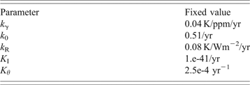
We now review the particle-filter algorithm. A particle is essentially a realisation of the state vector (say: y(t 0)) associated with a realisation of the parameters (A = {ln(ai,bi,ci)}) and a weight (w). Ten thousand (n) particles are initialised by sampling the prior of y(t 0) and A. Prior parameter distributions are log-normal around the values given in SM91 (Figure 7). Only the ai, bi, c 1 and k θ are considered to be uncertain, while the dissipative exchange coefficients KI and K θ as well as the climate sensitivities kμ and kR are assumed to be known (Table 1).
Prior (dashed) and posterior (full) density estimates of the parameters allowed to vary in SM91. The filter has been successful in narrowing down the distributions

Values of SM91 fixed parameters used both in the original publications and in the present article.
All weights are initialised to 1. The filter then consists of an iterative six-step process. Say we are at time t.
- Step 1.
Propagation, that is, time-integration of all particles until the time (t + 1) corresponding to the next available data (either CO2 or δ18O).
- Step 2.
Shrinkage. Particles are now dispersed in a region of the {Y, A}. This region is shrunk, that is, the particles are made closer to each other by a factor α.
- Step 3.
Weight estimate. Particle weights are multiplied by the likelihoods P(Z = z|Y = yj), where yj is the state of particle j, and z is the encountered data.
- Step 4.
Importance of resampling based on posterior estimate. After Step 2, some particles may be given a large weight while others only a small one. Particles are therefore resampled in such a way that they all get a similar weight. This implies that some particles are duplicated while others are killed. Particles are now distributed along k < n kernels.
- Step 5.
Resampling of kernels. Each kernel is broken apart into particles with parameters scattered with variance h 2.
- Step 6.
Weight update. Particles’ weights are updated according to their likelihood.
Shrinkage and kernel sampling are artefacts introduced to avoid filter degeneracy. Liu and WestReference Liu and West96 note that the estimator is unbiased for α = (3δ−1)/2δ and h 2 = 1−α 2. The parameter δ is called a discount factor. It must lie in [0,1] and typically be around 0.95–0.99. Here we choose δ = 0.95. We found that the parameter disturbance due to the filter dominates any reasonable amount of stochastic error that could be parameterised via W. Therefore, we decided not to account for the model stochastic error noise to gain computing efficiency.
Figure 8 summarises the essential features of the particle filter run. It represents, for each prognostic variable, the evolution of the state estimate (shaded) along with the data. The dark and light shades represent the central 50 and 90% percentiles of the weighted particle distribution. The filter algorithm updates the parameter estimates as it meets the data (The posterior parameter distributions are compared to the prior in Figure 7), which explains why the state estimates become narrowed as time progresses. The dots and pluses are the observation estimates of ice volume and CO2. The fourth panel is a first step towards model validation. It displays, for each observation, the model predictive probability that this observation was smaller or equal than its value, exactly in the spirit of equation (9). Values too close to zero or one cast doubt on the model.
Filtered state estimates with the SM91 model constrained by the SPECMAP data (squares), and the Antarctic ice core data (pluses). The state estimates are represented by shades, dark and light grey representing the [25th; 75th] and [5th; 95th] quantiles of the particle weighted distributions, respectively. The lower graph represents, for each data, the model predictive probability that the data would have been lower than it actually was, given the previous parameter and state estimates. The repetition of probabilities below 0.05 or above 0.95 tend to invalidate the model

It was unexpected that the fit of the state estimates of the ice volume on SPECMAP would be so poor. In fact, the model systematically overestimates ice volume during interglacials and this occurs as soon as CO2 observations are taken into account. Strictly speaking, the model is invalidated. Where does the problem lie?
The most obvious possibility is that we have incompletely modelled the SPECMAP stack. Indeed, we know that water temperature contributes to the δ18Oc signal but this contribution is missing in the model (Refs Reference Shackleton53,Reference Emiliani97–Reference Bintanja, van de Wal and Oerlemans99, the latest reference being another example of data reanalysis).
In spite of this weakness, we will assume that the model estimates of I’give a correct representation of ice volume anomalies around a tectonic time-scale average. Ice-volume levels typical of the last interglacial then correspond to I′ = −15 × 1018 m3 in the model. The model prediction is an immediate but slow decrease in CO2 concentration (Figure 8) but without glacial inception before about 50,000 years (this is the Berger and Loutre predictionReference Berger and Loutre9!). The particle filter also tells us that given the information at our disposal (the model, the data, and the parameter priors), it is not possible to provide a reliable estimate of the evolution of climate beyond 50,000 years.
What about Ruddiman’s hypothesis? Ruddiman considers that humans perturbed climate’s evolution around 8000 years ago. Therefore, we want to only consider data until that time, and see whether the model prediction differs from the previous one. The experiment was carried out and the results are presented on Figure 9. The grey boxes provide the prediction with data assimilated until 8,000 years ago, and the white ones are the prediction with data assimilated until today. The two predictions are clearly indistinguishable. Contrarily to Ruddiman, our model was therefore not ‘surprised’ by the fact that CO2 continued to increase during the last 6000 years.
State estimate with the SM91 model, given data on CO2 and ice volume between 410 kyr BP and 8 kyr BP (white) or 0 lyr BP (grey). The subsequent prediction, with glacial inception in 50 kyr, is little affected by the data between 8 and 0 kyr BP. This is opposed to Ruddiman’s hypothesis

Conclusion
Behind this paper is the message that climate modelling is not and should not be a mere technological question. Of course, general circulation models skilfully predict many complicated aspects of atmosphere and ocean dynamics; in that sense they are important and useful. Yet, they are but one aspect of the theoretical construct that underlies state-of-the-art knowledge of the climate system. Important questions are how we validate and calibrate climate models to provide the most informed predictions on climate change.
Palaeoclimates offer a premium playground to test the paradigms of complex system theory. We have been insistent on the fact that palaeoclimate theory must rely on two pillars of modern applied mathematics: dynamical system theory and statistical decision theory. Along with the fact that palaeoclimate data have to be interpreted and retrieved by skilful field scientists, their analysis turns to be a truly multidisciplinary experience. The exceptionally difficult challenges so posed are definitively at the frontier of knowledge.
Acknowledgements
The author would like to thank the organisers of the ‘Complexity’ workshop – Heidelberg for their kind invitation. The author would like also to thank Jonathan Rougier for his thoughtful comments on an earlier version of this paper.
Michel Crucifix graduated in Physics in Namur University (1998), followed by a Master in Physics (1999) and a doctorate in Sciences (2002) in Louvain-la-Neuve (Belgium). The subject of his thesis was ‘modelling glacial–interglacial climates over the last glacial-interglacial cycle’. The origin and mechanisms of glacial–interglacial cycles that have paced the Earth over the last million years has remained his favourite topic throughout his young career. He was appointed permanent research scientist at the Meteorological Office Hadley Centre (UK) in 2002 and then returned to Belgium, his home country, as a research associate with the Belgian national fund of scientific research, and lecturer in two universities (Louvain-la-Neuve and Namur).



