


1. Introduction
The study of complex systems through their interconnected elements has become central to numerous scientific disciplines. Such systems are commonly represented as networks or graphs, comprising autonomous actors (nodes) and the relational ties (edges) between them. These structures reveal patterns underlying phenomena ranging from disease transmission to social collaboration. The breadth of applications underscores the versatility of network models, which can represent entities as diverse as individuals, organizations, or nations, linked by relationships such as friendships, collaborations, or information exchange, respectively.
Modern statistical network analysis has three primary objectives: (1) identifying and summarizing structural patterns, (2) developing stochastic models to explain network formation processes, and (3) predicting unobserved or future connections based on network properties and actor attributes (see Pósfai and Barabási, Reference Pósfai and Barabási2016, Al-Taie and Kadry, Reference Al-Taie and Kadry2017, Newman, Reference Newman2018, Brugere et al., Reference Brugere, Gallagher and Berger-Wolf2018, and Drobyshevskiy and Turdakov, Reference Drobyshevskiy and Turdakov2019 for comprehensive reviews of network definitions, properties, methods, models, and processes across multiple fields). A central challenge lies in formulating statistical models (rather than deterministic mechanisms) that capture the inherent dependencies among ties, particularly reciprocity and transitivity. Traditional approaches, such as the exponential random graph models of Robins et al. (Reference Robins, Pattison, Kalish and Lusher2007), address these dependencies but are often susceptible to degeneracy and limited interpretability.
In statistical network modeling, latent space models offer a compelling alternative (see Goldenberg et al., Reference Goldenberg, Zheng, Fienberg and Airoldi2010, Salter-Townshend et al., Reference Salter-Townshend, White, Gollini and Murphy2012, Matias and Robin, Reference Matias, Robin, Abergel, Aiguier, Challet, Cournède, Faÿ and Lafitte2014, Sosa and Buitrago, Reference Sosa and Buitrago2021, and Kaur et al., Reference Kaur, Rastelli, Friel and Raftery2023 for comprehensive reviews of latent space modeling and related statistical approaches). In particular, the latent space model, introduced in the foundational work of Hoff et al. (Reference Hoff, Raftery and Handcock2002), embeds actors in an unobserved, typically low-dimensional, latent space (often referred to as the social space) where the probability of a tie is modeled as a function of the distance or similarity measure between actors in that space. This formulation naturally captures transitivity, as actors positioned closer together in latent space are more likely to form connections. The geometric structure of these models renders them both computationally tractable and interpretable. Nonetheless, they may be inadequate for networks generated by highly nonlinear processes or exhibiting complex geometric features beyond the representational capacity of Euclidean spaces.
Latent space models have been extensively extended to a wide range of settings. Beyond simple distance-based formulations, alternative latent structures have been proposed, including projection models (Hoff et al., Reference Hoff, Raftery and Handcock2002), bilinear models (Hoff, Reference Hoff2005, Hoff, Reference Hoff2021), and eigenmodels (Hoff, Reference Hoff2008, Hoff, Reference Hoff2009, Minhas et al., Reference Minhas, Hoff and Ward2019). These frameworks have been generalized to accommodate multiple structural features, such as multilayer networks (Hoff, Reference Hoff2011, Kivelä et al., Reference Kivelä, Arenas, Barthelemy, Gleeson, Moreno and Porter2014, Gollini and Murphy, Reference Gollini and Murphy2016, Salter-Townshend and McCormick, Reference Salter-Townshend and McCormick2017, D’Angelo et al., Reference D’Angelo, Murphy and Alfò2019, Zhang et al., Reference Zhang, Xue and Zhu2020, Sosa and Rodríguez, Reference Sosa and Rodríguez2021, Sosa and Betancourt, Reference Sosa and Betancourt2022, D’Angelo et al., Reference D’Angelo, Alfò and Fop2023) and dynamic network settings (Durante and Dunson, Reference Durante and Dunson2014, Sewell and Chen, Reference Sewell and Chen2015, Hoff, Reference Hoff2015, Sewell and Chen, Reference Sewell and Chen2016, Sewell and Chen, Reference Sewell and Chen2017, Kim et al., Reference Kim, Lee, Xue and Niu2018, He and Hoff, Reference He and Hoff2019, Guhaniyogi and Rodriguez, Reference Guhaniyogi and Rodriguez2020). They have also been adapted to perform diverse statistical tasks, including covariate testing (Austin et al., Reference Austin, Linkletter and Wu2013, Fosdick and Hoff, Reference Fosdick and Hoff2015, Wang et al., Reference Wang, Paul and De Boeck2023), clustering (Nowicki and Snijders, Reference Nowicki and Snijders2001, Krivitsky et al., Reference Krivitsky, Handcock, Raftery and Hoff2009, Ryan et al., Reference Ryan, Wyse and Friel2017, Rastelli and Friel, Reference Rastelli and Friel2018, Ng and Murphy, Reference Ng and Murphy2022), modeling bipartite relational data (Friel et al., Reference Friel, Rastelli, Wyse and Raftery2016), deduplication and record linkage (Sosa and Rodríguez, Reference Sosa and Rodríguez2022, Sosa and Rodríguez, Reference Sosa and Rodríguez2023), and the study of influence and diffusion processes (Xu, Reference Xu2018, Sánchez et al., Reference Sánchez, Sosa and Luque2026). Moreover, significant efforts have focused on developing faster computational alternatives to improve scalability and efficiency (Hunter et al., Reference Hunter, Krivitsky and Schweinberger2012, Raftery et al., Reference Raftery, Niu, Hoff and Yeung2012, Salter-Townshend and Murphy, Reference Salter-Townshend and Murphy2013, Caimo and Gollini, Reference Caimo and Gollini2016, Ma et al., Reference Ma, Ma and Yuan2020, Aliverti and Russo, Reference Aliverti and Russo2022, Spencer et al., Reference Spencer, Junker and Sweet2022, Rastelli et al., Reference Rastelli, Maire and Friel2024).
Most of these extensions adopt the standard choice of a Euclidean latent space, i.e. embedding actors in $\mathbb{R}^{d}$
for some positive integer
$\mathbb{R}^{d}$
for some positive integer $d$
, and model tie probabilities as decreasing functions of Euclidean distance. This specification is attractive for its simplicity and interpretability, but it has structural limitations that are important in some applications. First, the latent space is unbounded, so latent positions can move very far apart and this can produce extreme values in the linear predictor and almost deterministic tie probabilities, especially in very sparse or highly clustered networks. Second, the Euclidean formulation is invariant under global translation and rescaling of the configuration, so the overall scale of the latent positions is not identified separately from the intercept and other global parameters, which complicates prior specification and interpretation. Third, while Euclidean geometry is flexible and widely applicable, it can be less naturally suited to representing directional or cyclic organization. For example, when actors are arranged around ideological orientations or functional roles, a Euclidean embedding may require additional dimensions or ad hoc constraints to approximate the underlying structure, potentially reducing parsimony or interpretability. These considerations motivate the exploration of latent spaces with bounded geometry and a natural notion of angular similarity.
$d$
, and model tie probabilities as decreasing functions of Euclidean distance. This specification is attractive for its simplicity and interpretability, but it has structural limitations that are important in some applications. First, the latent space is unbounded, so latent positions can move very far apart and this can produce extreme values in the linear predictor and almost deterministic tie probabilities, especially in very sparse or highly clustered networks. Second, the Euclidean formulation is invariant under global translation and rescaling of the configuration, so the overall scale of the latent positions is not identified separately from the intercept and other global parameters, which complicates prior specification and interpretation. Third, while Euclidean geometry is flexible and widely applicable, it can be less naturally suited to representing directional or cyclic organization. For example, when actors are arranged around ideological orientations or functional roles, a Euclidean embedding may require additional dimensions or ad hoc constraints to approximate the underlying structure, potentially reducing parsimony or interpretability. These considerations motivate the exploration of latent spaces with bounded geometry and a natural notion of angular similarity.
One way to address these limitations is to embed actors on a hypersphere instead of in a flat geometry. The use of circular or spherical latent spaces in network modeling is well established in the literature. For example, Hoff et al. (Reference Hoff, Raftery and Handcock2002) introduced a projection model in which latent positions lie on the unit sphere and similarity is captured through angular structure. More recently, spherical and other non-Euclidean geometries have been studied in broader geometric frameworks for network models (e.g., McCormick and Zheng, Reference McCormick and Zheng2015; Smith et al., Reference Smith, Asta and Calder2019; Papamichalis et al., Reference Papamichalis, Turnbull, Lunagomez and Airoldi2022; Lubold et al., Reference Lubold, Chandrasekhar and McCormick2023), where curvature and manifold structure are treated as central modeling components. Our contribution builds on this line of work but differs in emphasis and scope. We focus on a latent distance model for general individual-level social network data in which the hypersphere is adopted as the primary latent space and inference is conducted within a Bayesian framework, implementing Markov chain Monte Carlo (MCMC) algorithms (e.g., Gamerman and Lopes, Reference Gamerman and Lopes2006) that explicitly respect the manifold constraints of spherical latent positions.
From a modeling perspective, the spherical geometry responds directly to the problems described above. By constraining all latent positions to lie on the unit sphere we fix the origin and the overall scale of the configuration, and the contribution of the latent space enters only through inner products in the interval $[\!-1,1]$
, which keeps the linear predictor in a moderate range and prevents tie probabilities from becoming numerically zero or one, stabilizing posterior inference and prediction. Similarity is captured through angular separation, so the geometry naturally represents directional clustering and cyclic structures and provides additional modeling flexibility in applications where actors are organized around latent directions. Angular separation also defines latent directions that correspond to interpretable groups or factions. In this paper we develop a general Bayesian inference framework for this spherical latent space model using MCMC and we demonstrate its performance on benchmark social network data sets, including those in Hoff et al. (Reference Hoff, Raftery and Handcock2002), where it demonstrates competitive model fit and enhanced geometric interpretability relative to the traditional Euclidean formulation. We do not claim that spherical geometry universally dominates Euclidean latent spaces. Rather, our objective is to demonstrate when a bounded and angular latent representation can provide computational stability, interpretability, and competitive predictive performance relative to standard Euclidean formulations using a benchmark example.
$[\!-1,1]$
, which keeps the linear predictor in a moderate range and prevents tie probabilities from becoming numerically zero or one, stabilizing posterior inference and prediction. Similarity is captured through angular separation, so the geometry naturally represents directional clustering and cyclic structures and provides additional modeling flexibility in applications where actors are organized around latent directions. Angular separation also defines latent directions that correspond to interpretable groups or factions. In this paper we develop a general Bayesian inference framework for this spherical latent space model using MCMC and we demonstrate its performance on benchmark social network data sets, including those in Hoff et al. (Reference Hoff, Raftery and Handcock2002), where it demonstrates competitive model fit and enhanced geometric interpretability relative to the traditional Euclidean formulation. We do not claim that spherical geometry universally dominates Euclidean latent spaces. Rather, our objective is to demonstrate when a bounded and angular latent representation can provide computational stability, interpretability, and competitive predictive performance relative to standard Euclidean formulations using a benchmark example.
In this spirit, the paper pursues three main goals. First, we formulate a spherical latent space model for social networks and develop simulation-based inference procedures that respect the geometry of the hypersphere using Metropolis and Hamiltonian based updates. Second, we carry out a detailed comparative analysis of Euclidean and spherical latent spaces on the Florentine marriage network as in Hoff et al. (Reference Hoff, Raftery and Handcock2002), evaluating model fit, recovery of centrality, community detection, and predictive performance. Finally, we provide free public code available at https://github.com/cnosa/Latentspacemodels_Networks, implementing all the sampling algorithms in plain Python, allowing direct modification and extension without reliance on automatic differentiation frameworks that assume unconstrained Euclidean parameter spaces. These contributions show that spherical latent space models provide an interpretable directional representation of network structure and achieve competitive predictive performance under a more constrained formulation.
The remainder of this article is structured as follows. Section 2 describes the fundamentals of network structures and their characterization, reviews related work on latent space modeling, and presents the proposed Euclidean and spherical latent space framework, along with its statistical properties. Section 3 details the Bayesian inference procedure and computational strategies. Section 4 presents the experimental results, and Section 5 concludes with an analysis of the implications and avenues for future research.
2. Fundamentals
Network data consist of actors, nodal attributes measured on individuals, and dyadic attributes measured on actor pairs. Dyadic variables may be binary, indicating the presence or absence of a tie (binary networks), or weighted, quantifying relational aspects (valued networks). Relations can be undirected, with a single value per pair, or directed, with two values capturing each actor’s perspective. Networks are typically represented as graphs or adjacency matrices $\mathbf{Y} = [y_{i,j}]$
, where
$\mathbf{Y} = [y_{i,j}]$
, where $y_{i,j}$
denotes the presence, absence, or weight of a tie. Self-loops generate structural zeros on the diagonal, and the symmetry or asymmetry of
$y_{i,j}$
denotes the presence, absence, or weight of a tie. Self-loops generate structural zeros on the diagonal, and the symmetry or asymmetry of $\mathbf{Y}$
indicates whether the network is undirected or directed.
$\mathbf{Y}$
indicates whether the network is undirected or directed.
Statistical network analysis methods fall into three categories: descriptive, which visualize and quantify structure; modeling and inference, which explain network formation; and process, which study how interactions influence attributes. This work focuses on modeling and inference, emphasizing structural features such as cohesion, connectivity, and assortativity that reflect dependencies like reciprocity and clustering. Accounting for these dependencies is crucial for constructing realistic statistical models. For comprehensive reviews of network properties and measures, see Menczer et al. (Reference Menczer, Fortunato and Davis2020) and Kolaczyk and Csárdi (Reference Kolaczyk and Csárdi2020).
In this context, a statistical network model is a probability distribution on a sociomatrix $\mathbf{Y}$
indexed by an unknown parameter
$\mathbf{Y}$
indexed by an unknown parameter $\boldsymbol{\theta } \in \Theta$
,
$\boldsymbol{\theta } \in \Theta$
, $p(\mathbf{Y} \mid \boldsymbol{\theta })$
. Rather than merely visualizing and describing the topological characteristics of a network, statistical models seek to capture the essential aspects of the stochastic mechanism by which the network may have arisen. They enable testing the significance of predefined structural features, assessing associations between node or edge attributes and the overall network structure, and imputing missing observations. Unlike deterministic or purely algorithmic models, statistical approaches also quantify the uncertainty associated with unknown quantities. Importantly, the very nature of network data induces dependencies both between actors and between ties. Accounting for these dependencies is indispensable for formulating statistically sound and substantively meaningful network models.
$p(\mathbf{Y} \mid \boldsymbol{\theta })$
. Rather than merely visualizing and describing the topological characteristics of a network, statistical models seek to capture the essential aspects of the stochastic mechanism by which the network may have arisen. They enable testing the significance of predefined structural features, assessing associations between node or edge attributes and the overall network structure, and imputing missing observations. Unlike deterministic or purely algorithmic models, statistical approaches also quantify the uncertainty associated with unknown quantities. Importantly, the very nature of network data induces dependencies both between actors and between ties. Accounting for these dependencies is indispensable for formulating statistically sound and substantively meaningful network models.
2.1 Latent space models
Latent space models are a widely used approach to network modeling, originally introduced by Hoff et al. (Reference Hoff, Raftery and Handcock2002) and further developed by Handcock et al. (Reference Handcock, Raftery and Tantrum2007) and Krivitsky et al. (Reference Krivitsky, Handcock, Raftery and Hoff2009). In this framework, each node is assigned a latent position in a Euclidean space, and the probability of an edge between two nodes depends on their proximity in that space. These models can be viewed as generalized linear models with random effects, allowing them to capture complex network structures. For conditionally independent $y_{i,j}$
in the undirected binary case, the interaction probabilities are
$y_{i,j}$
in the undirected binary case, the interaction probabilities are
 \begin{equation*} \textsf {Pr}(y_{i,j} = 1 \mid \mathbf{x}_{i,j}, \boldsymbol{\beta }, \zeta _{i,j}) = \textsf {logit}^{-1}\big(\mathbf{x}^{\top} _{i,j}\boldsymbol{\beta } + \zeta _{i,j}\big), \qquad 1 \leq i \lt j \leq n, \end{equation*}
where $\boldsymbol{\beta }$
are fixed effects,
$\boldsymbol{\beta }$
are fixed effects, $\mathbf{x}^{\top} _{i,j}\boldsymbol{\beta }$
represents the contribution of covariates
$\mathbf{x}^{\top} _{i,j}\boldsymbol{\beta }$
represents the contribution of covariates $\mathbf{x}_{i,j}$
, and
$\mathbf{x}_{i,j}$
, and $\zeta _{i,j}$
captures unobserved effects, and
$\zeta _{i,j}$
captures unobserved effects, and $\textsf {logit}(x) = \log \frac {x}{1-x}$
is the link function. As noted in Hoff (Reference Hoff2008), following foundational results from Hoover (Reference Hoover1982) and Aldous (Reference Aldous1985), a jointly exchangeable random effects matrix
$\textsf {logit}(x) = \log \frac {x}{1-x}$
is the link function. As noted in Hoff (Reference Hoff2008), following foundational results from Hoover (Reference Hoover1982) and Aldous (Reference Aldous1985), a jointly exchangeable random effects matrix $[\zeta _{i,j}]$
can be expressed as
$[\zeta _{i,j}]$
can be expressed as $\zeta _{i,j} = h(\mathbf{z}_i, \mathbf{z}_j)$
, where
$\zeta _{i,j} = h(\mathbf{z}_i, \mathbf{z}_j)$
, where $h(\cdot ,\cdot )$
is a symmetric function and
$h(\cdot ,\cdot )$
is a symmetric function and $\mathbf{z}_1, \ldots , \mathbf{z}_n$
are independent latent variables (vectors). The function
$\mathbf{z}_1, \ldots , \mathbf{z}_n$
are independent latent variables (vectors). The function $h(\cdot ,\cdot )$
is central to modeling relational data, and various formulations have been proposed. In this paper, we focus on the distance formulation for undirected binary networks. For a comprehensive review, see Sosa and Buitrago (Reference Sosa and Buitrago2021).
$h(\cdot ,\cdot )$
is central to modeling relational data, and various formulations have been proposed. In this paper, we focus on the distance formulation for undirected binary networks. For a comprehensive review, see Sosa and Buitrago (Reference Sosa and Buitrago2021).
A common specification is the latent distance model (Hoff et al., Reference Hoff, Raftery and Handcock2002), in which each actor $i$
occupies an unobserved position
$i$
occupies an unobserved position $\mathbf{z}_i \in \mathbb{R}^d$
, often referred to as the latent or social space. Conditional on these positions, ties are modeled as
$\mathbf{z}_i \in \mathbb{R}^d$
, often referred to as the latent or social space. Conditional on these positions, ties are modeled as
 \begin{equation*} y_{i,j} \mid \eta _{i,j} \overset {\text{ind}}{\sim } \textsf {Ber}\big (\textsf {logit}^{-1}(\eta _{i,j})\big ), \qquad \eta _{i,j} = \alpha - \textsf {d}(\mathbf{z}_i, \mathbf{z}_j), \end{equation*}
where $\mathbf{z}_i$
and
$\mathbf{z}_i$
and $\mathbf{z}_j$
are latent position vectors capturing unobserved social characteristics,
$\mathbf{z}_j$
are latent position vectors capturing unobserved social characteristics, $\textsf {d}(\cdot ,\cdot )$
is a distance function, typically
$\textsf {d}(\cdot ,\cdot )$
is a distance function, typically $\textsf {d}(\mathbf{z}_i, \mathbf{z}_j) = \| \mathbf{z}_i - \mathbf{z}_j \|$
with
$\textsf {d}(\mathbf{z}_i, \mathbf{z}_j) = \| \mathbf{z}_i - \mathbf{z}_j \|$
with $\|\cdot \|$
denoting the Euclidean norm in
$\|\cdot \|$
denoting the Euclidean norm in $\mathbb{R}^d$
, and
$\mathbb{R}^d$
, and $\alpha$
is an intercept representing the baseline log odds of a tie when two actors occupy the same latent position. The subtraction of
$\alpha$
is an intercept representing the baseline log odds of a tie when two actors occupy the same latent position. The subtraction of $\textsf {d}(\mathbf{z}_i, \mathbf{z}_j)$
from
$\textsf {d}(\mathbf{z}_i, \mathbf{z}_j)$
from $\alpha$
reflects the assumption that the probability of a tie decreases as the distance between latent positions increases, encouraging connections between actors located close together in latent space. This property naturally induces transitivity and clustering, as actors close to a common neighbor are also likely to be close to each other.
$\alpha$
reflects the assumption that the probability of a tie decreases as the distance between latent positions increases, encouraging connections between actors located close together in latent space. This property naturally induces transitivity and clustering, as actors close to a common neighbor are also likely to be close to each other.
Alternatively, for modeling in a spherical latent space, the probability of a tie can be parameterized using the inner product between latent vectors, capturing proximity through angular similarity:
 \begin{equation*} \eta _{i,j} = \textsf {logit} \, \textsf {P}(y_{i,j} = 1 \mid \alpha ,\beta , \mathbf{z}_i, \mathbf{z}_j) = \alpha + \beta \, \langle \mathbf{z}_i, \mathbf{z}_j \rangle , \end{equation*}
where $\mathbf{z}_i, \mathbf{z}_j \in \mathbb{S}^{d-1}$
are unit vectors on the
$\mathbf{z}_i, \mathbf{z}_j \in \mathbb{S}^{d-1}$
are unit vectors on the $(d-1)$
-dimensional sphere,
$(d-1)$
-dimensional sphere, $\langle \mathbf{z}_i, \mathbf{z}_j \rangle = \mathbf{z}_i^{\top} \mathbf{z}_j$
denotes the standard inner product in
$\langle \mathbf{z}_i, \mathbf{z}_j \rangle = \mathbf{z}_i^{\top} \mathbf{z}_j$
denotes the standard inner product in $\mathbb{S}^{d-1}$
,
$\mathbb{S}^{d-1}$
, $\alpha$
is an intercept representing the baseline log odds of a tie when the latent vectors are orthogonal, and
$\alpha$
is an intercept representing the baseline log odds of a tie when the latent vectors are orthogonal, and $\beta$
is a scaling parameter controlling how strongly angular similarity influences tie formation. Geometrically,
$\beta$
is a scaling parameter controlling how strongly angular similarity influences tie formation. Geometrically, $\beta$
determines how sharply the log odds change as the angle between
$\beta$
determines how sharply the log odds change as the angle between $\mathbf{z}_i$
and
$\mathbf{z}_i$
and $\mathbf{z}_j$
decreases: larger values of
$\mathbf{z}_j$
decreases: larger values of $\beta$
make the probability of a tie increase more rapidly as the two latent positions align. Lastly, we emphasize that, analogous to the Euclidean latent distance model, the latent positions
$\beta$
make the probability of a tie increase more rapidly as the two latent positions align. Lastly, we emphasize that, analogous to the Euclidean latent distance model, the latent positions $\mathbf{z}_1,\ldots ,\mathbf{z}_n$
serve as embeddings of actors that capture unobserved affinities, providing a foundation for visualization, clustering, and structural analysis of the network.
$\mathbf{z}_1,\ldots ,\mathbf{z}_n$
serve as embeddings of actors that capture unobserved affinities, providing a foundation for visualization, clustering, and structural analysis of the network.
We constrain the latent positions to the $(d-1)$
-dimensional unit sphere
$(d-1)$
-dimensional unit sphere $\mathbb{S}^{d-1}$
, which fixes the origin and scale of the configuration, removing translation and scaling invariances, reducing each position’s degrees of freedom from
$\mathbb{S}^{d-1}$
, which fixes the origin and scale of the configuration, removing translation and scaling invariances, reducing each position’s degrees of freedom from $d$
to
$d$
to $d-1$
, and thus ensuring identifiability up to a global rotation (see Section 2.2 for details). On
$d-1$
, and thus ensuring identifiability up to a global rotation (see Section 2.2 for details). On $\mathbb{S}^{d-1}$
, the inner product
$\mathbb{S}^{d-1}$
, the inner product $\langle \mathbf{z}_i, \mathbf{z}_j \rangle = \cos (\gamma _{i,j})$
relates directly to the geodesic distance
$\langle \mathbf{z}_i, \mathbf{z}_j \rangle = \cos (\gamma _{i,j})$
relates directly to the geodesic distance $\gamma _{i,j}$
, defined here as the intrinsic (angular) distance on the sphere. We use the cosine similarity
$\gamma _{i,j}$
, defined here as the intrinsic (angular) distance on the sphere. We use the cosine similarity $\langle \mathbf{z}_i, \mathbf{z}_j \rangle$
rather than
$\langle \mathbf{z}_i, \mathbf{z}_j \rangle$
rather than $\gamma _{i,j} = \arccos \,\langle \mathbf{z}_i, \mathbf{z}_j \rangle$
to avoid the numerical instability of the
$\gamma _{i,j} = \arccos \,\langle \mathbf{z}_i, \mathbf{z}_j \rangle$
to avoid the numerical instability of the $\arccos$
gradient. The spherical formulation yields a compact latent space, preventing positions from drifting to arbitrarily large norms as in Euclidean spaces, thereby avoiding degeneracy and improving numerical stability.
$\arccos$
gradient. The spherical formulation yields a compact latent space, preventing positions from drifting to arbitrarily large norms as in Euclidean spaces, thereby avoiding degeneracy and improving numerical stability.
In Hoff et al., (Reference Hoff, Raftery and Handcock2002, Sec. 2.2), the projection model, which is related but distinct from our approach, specifies
 \begin{equation*} \eta _{i,j} = \alpha + \frac {\mathbf z_i^{\top} \mathbf z_j}{\|\mathbf z_j\|}, \end{equation*}
so the likelihood depends on the configuration $\{\mathbf z_i\}$
through inner products and norms in an unconstrained Euclidean space. As stated by Hoff et al. (Reference Hoff, Raftery and Handcock2002), this model is invariant under common rotations and reflections of the latent positions, but not under translations and not under global rescaling. In our spherical specification the latent positions are constrained to lie on the unit sphere,
$\{\mathbf z_i\}$
through inner products and norms in an unconstrained Euclidean space. As stated by Hoff et al. (Reference Hoff, Raftery and Handcock2002), this model is invariant under common rotations and reflections of the latent positions, but not under translations and not under global rescaling. In our spherical specification the latent positions are constrained to lie on the unit sphere, $\mathbf z_i \in \mathbb S^{d-1}$
, and the linear predictor depends on them only through the inner product
$\mathbf z_i \in \mathbb S^{d-1}$
, and the linear predictor depends on them only through the inner product $\langle \mathbf z_i , \mathbf z_j \rangle = \cos (\gamma _{i,j})$
, where
$\langle \mathbf z_i , \mathbf z_j \rangle = \cos (\gamma _{i,j})$
, where $\gamma _{i,j}$
is the geodesic distance. The spherical constraint thus fixes both the location and the overall scale of the configuration and leaves only global rotations and reflections as symmetries, which in turn simplifies identifiability and the interpretation of the latent positions, reduces each position to
$\gamma _{i,j}$
is the geodesic distance. The spherical constraint thus fixes both the location and the overall scale of the configuration and leaves only global rotations and reflections as symmetries, which in turn simplifies identifiability and the interpretation of the latent positions, reduces each position to $d-1$
free parameters, and prevents norms from diverging.
$d-1$
free parameters, and prevents norms from diverging.
Given the conditional independence of connections given the intercept term and latent positions, the likelihood is
 \begin{equation*} \mathcal{L}(\alpha , \beta , \mathbf{Z}) = \prod _{i \lt j} p_{i,j}^{\,y_{i,j}} \left (1 - p_{i,j}\right )^{1 - y_{i,j}}\!, \end{equation*}
where $p_{i,j} = \textsf {logit}^{-1}\left (\eta _{i,j}\right ) = \textsf {logit}^{-1}\left (\alpha + \beta \,\langle \mathbf{z}_i, \mathbf{z}_j \rangle \right )$
is the interaction probability between nodes
$p_{i,j} = \textsf {logit}^{-1}\left (\eta _{i,j}\right ) = \textsf {logit}^{-1}\left (\alpha + \beta \,\langle \mathbf{z}_i, \mathbf{z}_j \rangle \right )$
is the interaction probability between nodes $i$
and
$i$
and $j$
, and
$j$
, and $\mathbf{Z} \in \mathbb{S}^{(d-1) \times n}$
is the matrix of latent positions with
$\mathbf{Z} \in \mathbb{S}^{(d-1) \times n}$
is the matrix of latent positions with $\|\mathbf{z}_i\|=1$
. Recall that the inner product
$\|\mathbf{z}_i\|=1$
. Recall that the inner product $\langle \mathbf{z}_i, \mathbf{z}_j \rangle$
equals
$\langle \mathbf{z}_i, \mathbf{z}_j \rangle$
equals $\cos (\gamma _{i,j})$
, where
$\cos (\gamma _{i,j})$
, where $\gamma _{i,j}$
is the geodesic distance on the sphere, so similarity is modeled directly via cosine values rather than angular distances. Thus, the log-likelihood takes the form
$\gamma _{i,j}$
is the geodesic distance on the sphere, so similarity is modeled directly via cosine values rather than angular distances. Thus, the log-likelihood takes the form
 \begin{equation*} \ell (\alpha ,\beta ,\mathbf{Z}) = \sum _{i \lt j} \left [ y_{i,j} \,\eta _{i,j} - \log \left ( 1 + e^{\eta _{i,j}} \right ) \right ], \end{equation*}
with $\eta _{i,j} = \alpha + \beta \,\langle \mathbf{z}_i, \mathbf{z}_j \rangle$
, for which the corresponding gradients are given by
$\eta _{i,j} = \alpha + \beta \,\langle \mathbf{z}_i, \mathbf{z}_j \rangle$
, for which the corresponding gradients are given by
 \begin{align*} \frac {\partial }{\partial \mathbf{z}_k} \,\ell (\alpha , \beta , \mathbf{Z}) &= \sum _{i \neq k} \left [ y_{i,k} - \textsf {expit}(\eta _{i,k}) \right ] \frac {\partial \eta _{i,k}}{\partial \mathbf{z}_k}, \\ \frac {\partial }{\partial \alpha } \,\ell (\alpha , \beta , \mathbf{Z}) &= \sum _{i \lt j} \left [ y_{i,j} - \textsf {expit}(\eta _{i,j}) \right ], \\ \frac {\partial }{\partial \beta } \,\ell (\alpha , \beta , \mathbf{Z}) &= \sum _{i \lt j} \left [ y_{i,j} - \textsf {expit}(\eta _{i,j}) \right ] \langle \mathbf{z}_i, \mathbf{z}_j \rangle . \end{align*}
Analogous expressions can be derived for the Euclidean latent distance model.
2.2 Model properties
Latent space models are non-identifiable because the linear predictor is invariant under specific transformations of the latent space. In particular, the likelihood function $\mathcal{L}$
remains unchanged under certain transformations applied to the
$\mathcal{L}$
remains unchanged under certain transformations applied to the $d \times n$
matrix
$d \times n$
matrix $\mathbf{Z}$
containing the latent positions. Such transformations generate equivalence classes of configurations of
$\mathbf{Z}$
containing the latent positions. Such transformations generate equivalence classes of configurations of $\mathbf{Z}$
that produce identical likelihood values.
$\mathbf{Z}$
that produce identical likelihood values.
In the Euclidean formulation, the model is invariant under isometries in $\mathbb{R}^d$
of the form
$\mathbb{R}^d$
of the form $\mathbf{Z} \mapsto \mathbf{Z}^{\prime} = \mathbf{Q} \mathbf{Z} + \mathbf{b}\mathbf{1}_n^{\top}$
, where
$\mathbf{Z} \mapsto \mathbf{Z}^{\prime} = \mathbf{Q} \mathbf{Z} + \mathbf{b}\mathbf{1}_n^{\top}$
, where $\mathbf{Q} \in \mathbb{R}^{d\times d}$
is orthogonal, representing a rotation or reflection,
$\mathbf{Q} \in \mathbb{R}^{d\times d}$
is orthogonal, representing a rotation or reflection, $\mathbf{b} \in \mathbb{R}^d$
is a translation vector applied uniformly to all points, and
$\mathbf{b} \in \mathbb{R}^d$
is a translation vector applied uniformly to all points, and $\mathbf{1}_n \in \mathbb{R}^n$
is a column vector of ones. Indeed, for transformed latent positions
$\mathbf{1}_n \in \mathbb{R}^n$
is a column vector of ones. Indeed, for transformed latent positions $\mathbf{z}_i^{\prime} = \mathbf{Q} \mathbf{z}_i + \mathbf{b}$
and
$\mathbf{z}_i^{\prime} = \mathbf{Q} \mathbf{z}_i + \mathbf{b}$
and $\mathbf{z}_j^{\prime} = \mathbf{Q} \mathbf{z}_j + \mathbf{b}$
, we have
$\mathbf{z}_j^{\prime} = \mathbf{Q} \mathbf{z}_j + \mathbf{b}$
, we have
 \begin{equation*} \|\mathbf{z}_i^{\prime} - \mathbf{z}_j^{\prime}\| = \| (\mathbf{Q} \mathbf{z}_i + \mathbf{b}) - (\mathbf{Q} \mathbf{z}_j + \mathbf{b}) \| = \|\mathbf{Q} (\mathbf{z}_i - \mathbf{z}_j)\| = \|\mathbf{z}_i - \mathbf{z}_j\|, \end{equation*}
since $\|\mathbf{Q} \mathbf{z}\| = \|\mathbf{z}\|$
, for any
$\|\mathbf{Q} \mathbf{z}\| = \|\mathbf{z}\|$
, for any $\mathbf{z} \in \mathbb{R}^d$
when
$\mathbf{z} \in \mathbb{R}^d$
when $\mathbf{Q}$
is orthogonal. Hence, all pairwise distances are preserved, and therefore,
$\mathbf{Q}$
is orthogonal. Hence, all pairwise distances are preserved, and therefore, $\mathcal{L}(\alpha , \mathbf{Z}) = \mathcal{L}(\alpha , \mathbf{Z}^{\prime})$
, inducing equivalence classes of
$\mathcal{L}(\alpha , \mathbf{Z}) = \mathcal{L}(\alpha , \mathbf{Z}^{\prime})$
, inducing equivalence classes of $\mathbf{Z}$
that yield identical likelihoods and making the latent positions non-identifiable without further constraints.
$\mathbf{Z}$
that yield identical likelihoods and making the latent positions non-identifiable without further constraints.
In the spherical formulation, the latent positions are constrained to the $(d-1)$
-dimensional unit sphere
$(d-1)$
-dimensional unit sphere $\mathbb{S}^{d-1} \subset \mathbb{R}^d$
, fixing both the origin and the scale of the configuration, removing translation and scaling invariances, and reducing each position’s degrees of freedom from
$\mathbb{S}^{d-1} \subset \mathbb{R}^d$
, fixing both the origin and the scale of the configuration, removing translation and scaling invariances, and reducing each position’s degrees of freedom from $d$
to
$d$
to $d-1$
. However, the model remains invariant under global orthogonal transformations
$d-1$
. However, the model remains invariant under global orthogonal transformations $\mathbf{Z} \mapsto \mathbf{Z}^{\prime} = \mathbf{Q} \mathbf{Z}$
, where
$\mathbf{Z} \mapsto \mathbf{Z}^{\prime} = \mathbf{Q} \mathbf{Z}$
, where $\mathbf{Q} \in \mathbb{R}^{d\times d}$
is orthogonal, representing rotations or reflections that preserve both geodesic distances and inner products on the sphere. Indeed, for transformed positions
$\mathbf{Q} \in \mathbb{R}^{d\times d}$
is orthogonal, representing rotations or reflections that preserve both geodesic distances and inner products on the sphere. Indeed, for transformed positions $\mathbf{z}_i^{\prime} = \mathbf{Q} \mathbf{z}_i$
and
$\mathbf{z}_i^{\prime} = \mathbf{Q} \mathbf{z}_i$
and $\mathbf{z}_j^{\prime} = \mathbf{Q} \mathbf{z}_j$
, we have
$\mathbf{z}_j^{\prime} = \mathbf{Q} \mathbf{z}_j$
, we have $\|\mathbf{z}_i^{\prime}\| = \|\mathbf{Q} \mathbf{z}_i\| = \|\mathbf{z}_i\| = 1$
, so the unit norm is preserved. Moreover,
$\|\mathbf{z}_i^{\prime}\| = \|\mathbf{Q} \mathbf{z}_i\| = \|\mathbf{z}_i\| = 1$
, so the unit norm is preserved. Moreover,
 \begin{equation*} \mathbf{z}_i^{\prime \top} \mathbf{z}_j^{\prime} = (\mathbf{Q} \mathbf{z}_i)^{\top} (\mathbf{Q} \mathbf{z}_j) = \mathbf{z}_i^{\top} \mathbf{Q}^{\top} \mathbf{Q} \mathbf{z}_j = \mathbf{z}_i^{\top} \mathbf{z}_j, \end{equation*}
so all pairwise inner products, and therefore all geodesic distances, are preserved. Consequently, $\mathcal{L}(\alpha , \beta , \mathbf{Z}) = \mathcal{L}(\alpha , \beta , \mathbf{Q} \mathbf{Z})$
, and the configuration is identifiable only up to a global rotation or reflection. This does not affect inference about relative positions but requires post-processing (e.g., Procrustes alignment, see Borg and Groenen, Reference Borg and Groenen2005 for an in-depth discussion) for visualization and interpretation.
$\mathcal{L}(\alpha , \beta , \mathbf{Z}) = \mathcal{L}(\alpha , \beta , \mathbf{Q} \mathbf{Z})$
, and the configuration is identifiable only up to a global rotation or reflection. This does not affect inference about relative positions but requires post-processing (e.g., Procrustes alignment, see Borg and Groenen, Reference Borg and Groenen2005 for an in-depth discussion) for visualization and interpretation.
2.3 Model extensions
In addition to the baseline spherical latent distance model, the framework admits several natural extensions. One direction is to include node specific random effects or covariate terms in the linear predictor in order to capture degree heterogeneity and assortative mixing beyond what is encoded by the latent positions. Another is to adapt the model to multilayer or multiplex networks by sharing or correlating latent positions across layers while allowing layer specific parameters. A third direction is to consider dynamic networks in which latent positions evolve over time according to a stochastic process on the sphere. These extensions are outlined in more detail in Appendix B, where we provide the corresponding formulations and discuss their potential applications.
3. Inference and computation
The Euclidean and spherical formulations of latent space models introduced above involve the intercept parameter $\alpha$
, the scaling parameter
$\alpha$
, the scaling parameter $\beta$
, and the matrix of latent positions
$\beta$
, and the matrix of latent positions $\mathbf{Z}$
, which together determine the structure of the observed network. Once the model formulation is complete, the next step is to estimate these parameters given the observed network data
$\mathbf{Z}$
, which together determine the structure of the observed network. Once the model formulation is complete, the next step is to estimate these parameters given the observed network data $\mathbf{Y}$
. This section provides a detailed treatment of both classical and Bayesian inference approaches, covering optimization techniques for point estimation as well as sampling algorithms for full posterior inference. All inference procedures described in this section are implemented in an open-source Python repository available at https://github.com/cnosa/Latentspacemodels_Networks.
$\mathbf{Y}$
. This section provides a detailed treatment of both classical and Bayesian inference approaches, covering optimization techniques for point estimation as well as sampling algorithms for full posterior inference. All inference procedures described in this section are implemented in an open-source Python repository available at https://github.com/cnosa/Latentspacemodels_Networks.
3.1 Classical inference
Here, we conduct classical inference via maximum likelihood estimation (e.g., Casella and Berger, Reference Casella and Berger2024), which we use primarily to obtain initial values for the latent positions and model parameters before applying MCMC-based algorithm. In latent space models, the likelihood function is generally not globally concave. This non-concavity complicates classical inference, as multiple local maxima necessitate iterative optimization methods and carefully selected initialization strategies to mitigate the risk of suboptimal convergence. To obtain the maximizer of the log-likelihood, we use gradient descent with a backtracking line search based on the Armijo condition (see Boyd and Vandenberghe, Reference Boyd and Vandenberghe2004 and Nocedal and Wright, Reference Nocedal and Wright2006), ensuring sufficient decrease of the objective at each iteration even in non-concave settings.
Let $\ell (\theta , \mathbf{Z})$
denote the log-likelihood, viewed as a function of the latent positions
$\ell (\theta , \mathbf{Z})$
denote the log-likelihood, viewed as a function of the latent positions $\mathbf{Z}$
and the other model parameters collected in
$\mathbf{Z}$
and the other model parameters collected in $\theta$
. Starting from initial values
$\theta$
. Starting from initial values $(\theta ^{(0)}, \mathbf{Z}^{(0)})$
, the parameters are updated jointly as
$(\theta ^{(0)}, \mathbf{Z}^{(0)})$
, the parameters are updated jointly as
 \begin{equation*} \big(\theta ^{(b+1)}, \mathbf{Z}^{(b+1)}\big) = \big(\theta ^{(b)}, \mathbf{Z}^{(b)}\big) + r^{(b)} \mathbf{D}^{(b)}, \end{equation*}
where $\mathbf{D}^{(b)} = \nabla \ell (\theta ^{(b)}, \mathbf{Z}^{(b)})$
is the gradient of the log-likelihood with respect to all model parameters, and
$\mathbf{D}^{(b)} = \nabla \ell (\theta ^{(b)}, \mathbf{Z}^{(b)})$
is the gradient of the log-likelihood with respect to all model parameters, and $r^{(b)}$
is a step size chosen to satisfy the Armijo condition
$r^{(b)}$
is a step size chosen to satisfy the Armijo condition
 \begin{equation*} \ell \big(\theta ^{(b+1)}, \mathbf{Z}^{(b+1)}\big) \geq \ell \big(\theta ^{(b)}, \mathbf{Z}^{(b)}\big) + c\, r^{(b)} \nabla \ell \big(\theta ^{(b)}, \mathbf{Z}^{(b)}\big)^{\top} \mathbf{D}^{(b)}, \end{equation*}
for some constant $c \in (0,1)$
. This ensures a sufficient ascent in the log-likelihood at each step while preserving convergence guarantees.
$c \in (0,1)$
. This ensures a sufficient ascent in the log-likelihood at each step while preserving convergence guarantees.
Because the log-likelihood landscape is highly sensitive to initialization, we examine multiple choices for the starting point $(\theta ^{(0)}, \mathbf{Z}^{(0)})$
, including random configurations. In the spherical model, optimization is additionally constrained by the manifold geometry, requiring each latent position to remain on the unit sphere. This is enforced by projecting the updated positions back onto the sphere after each gradient step. The procedure is summarized in Algorithm 1. Given these challenges and the model’s structure, classical inference may not always produce reliable or interpretable estimates. This motivates the use of Bayesian inference, which not only accounts for parameter uncertainty but also incorporates regularization naturally through the prior distribution on the model parameters.
$(\theta ^{(0)}, \mathbf{Z}^{(0)})$
, including random configurations. In the spherical model, optimization is additionally constrained by the manifold geometry, requiring each latent position to remain on the unit sphere. This is enforced by projecting the updated positions back onto the sphere after each gradient step. The procedure is summarized in Algorithm 1. Given these challenges and the model’s structure, classical inference may not always produce reliable or interpretable estimates. This motivates the use of Bayesian inference, which not only accounts for parameter uncertainty but also incorporates regularization naturally through the prior distribution on the model parameters.
Gradient ascent with Armijo backtracking line search for maximum likelihood estimation in latent space models

3.2 Bayesian inference
Bayesian inference offers a flexible alternative to traditional statistical learning methods (e.g., Gelman et al., Reference Gelman, Carlin, Stern, Dunson, Vehtari and Rubin2013a), providing both parameter estimation and uncertainty quantification through the full posterior distribution $p(\theta , \mathbf{Z} \mid \mathbf{Y})$
. To perform full Bayesian inference, it is first necessary to specify a sensible prior distribution
$p(\theta , \mathbf{Z} \mid \mathbf{Y})$
. To perform full Bayesian inference, it is first necessary to specify a sensible prior distribution $p(\theta , \mathbf{Z})$
. To do so, we adopt independent priors for the latent positions
$p(\theta , \mathbf{Z})$
. To do so, we adopt independent priors for the latent positions $\mathbf{z}_1, \ldots , \mathbf{z}_n$
, chosen to encode plausible assumptions about their spatial configuration before observing the data, and separately assign a prior distribution to the remaining model parameters collected in
$\mathbf{z}_1, \ldots , \mathbf{z}_n$
, chosen to encode plausible assumptions about their spatial configuration before observing the data, and separately assign a prior distribution to the remaining model parameters collected in $\theta$
. These priors regularize while respecting the model’s invariances, preventing degeneracy and stabilizing computation.
$\theta$
. These priors regularize while respecting the model’s invariances, preventing degeneracy and stabilizing computation.
In the Euclidean case, we assign an isotropic Gaussian prior to the latent positions,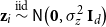 $\mathbf{z}_{i} \overset {\text{iid}}{\sim } \mathsf{N} \big (\mathbf{0}, \sigma _{z}^{2}\,\mathbf{I}_{d}\big )$
, for
$\mathbf{z}_{i} \overset {\text{iid}}{\sim } \mathsf{N} \big (\mathbf{0}, \sigma _{z}^{2}\,\mathbf{I}_{d}\big )$
, for $i = 1, \ldots , n$
, and independently set
$i = 1, \ldots , n$
, and independently set $\alpha \sim \mathsf{N} \big (\mu _\alpha , \sigma _{\alpha }^{2}\big )$
. This prior is rotationally and translationally symmetric, aligning with the likelihood’s invariance under orthogonal transformations. It avoids directional bias, preserves the geometry of the latent space, and softly shrinks positions toward the origin, thereby controlling the unbounded nature of Euclidean embeddings and preventing norm divergence.
$\alpha \sim \mathsf{N} \big (\mu _\alpha , \sigma _{\alpha }^{2}\big )$
. This prior is rotationally and translationally symmetric, aligning with the likelihood’s invariance under orthogonal transformations. It avoids directional bias, preserves the geometry of the latent space, and softly shrinks positions toward the origin, thereby controlling the unbounded nature of Euclidean embeddings and preventing norm divergence.
In the spherical case, we place a uniform prior on the hypersphere, $\mathbf{z}_{i} \overset {\text{iid}}{\sim } \mathsf{U} (\mathbb{S}^{d-1} )$
, for
$\mathbf{z}_{i} \overset {\text{iid}}{\sim } \mathsf{U} (\mathbb{S}^{d-1} )$
, for $i = 1, \ldots , n$
, and a correlated Gaussian prior on
$i = 1, \ldots , n$
, and a correlated Gaussian prior on $(\alpha , \beta )$
with
$(\alpha , \beta )$
with $\alpha \sim \mathsf{N} (\mu _\alpha , \sigma _{\alpha }^2 )$
,
$\alpha \sim \mathsf{N} (\mu _\alpha , \sigma _{\alpha }^2 )$
, $\beta \sim \mathsf{N} (\mu _\beta , \sigma _{\beta }^2)$
, and
$\beta \sim \mathsf{N} (\mu _\beta , \sigma _{\beta }^2)$
, and $\textsf {Cov}(\alpha , \beta ) = \rho \,\sigma _{\alpha }\sigma _{\beta }$
. The joint prior on
$\textsf {Cov}(\alpha , \beta ) = \rho \,\sigma _{\alpha }\sigma _{\beta }$
. The joint prior on $(\alpha ,\beta )$
allows for prior dependence between baseline tie propensity and the strength of the latent space term, since both influence overall network density in logistic latent space models. This motivates a bivariate normal prior with unrestricted covariance rather than independent priors. In practice, however, empirical results are essentially unchanged under independent normal priors, so readers who prefer a simpler specification can safely use independent priors for
$(\alpha ,\beta )$
allows for prior dependence between baseline tie propensity and the strength of the latent space term, since both influence overall network density in logistic latent space models. This motivates a bivariate normal prior with unrestricted covariance rather than independent priors. In practice, however, empirical results are essentially unchanged under independent normal priors, so readers who prefer a simpler specification can safely use independent priors for $\alpha$
and
$\alpha$
and $\beta$
. The uniform prior corresponds to the uniform measure on
$\beta$
. The uniform prior corresponds to the uniform measure on $\mathbb{S}^{d-1}$
, ensuring invariance under all orthogonal transformations in
$\mathbb{S}^{d-1}$
, ensuring invariance under all orthogonal transformations in $\mathbb{R}^d$
. This symmetry makes all orientations of the latent configuration equally likely, fully respecting the rotational and reflectional invariance of the spherical latent space.
$\mathbb{R}^d$
. This symmetry makes all orientations of the latent configuration equally likely, fully respecting the rotational and reflectional invariance of the spherical latent space.
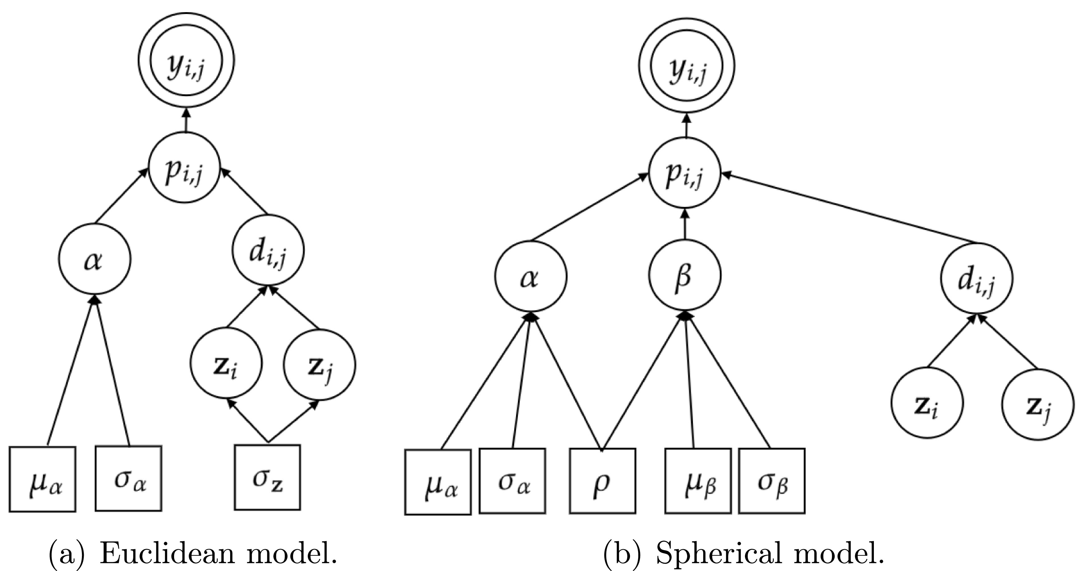
To clarify the probabilistic structure of the models, we present in Figure 1 the directed acyclic graphs (DAGs) corresponding to both the Euclidean and spherical formulations. These graphical representations explicitly illustrate the conditional dependencies among observed ties, latent positions, and global parameters, making clear the conditional independence assumptions underlying the model specification.
Directed acyclic graphs (DAGs) for the latent space models, where circles denote random variables or random vectors, squares indicate fixed parameters, and edges represent dependencies.
Under the prior specifications given above, let the interaction probabilities be defined as $p_{i,j} = \textsf {logit}^{-1}(\eta _{i,j})$
, where
$p_{i,j} = \textsf {logit}^{-1}(\eta _{i,j})$
, where $\eta _{i,j} = \eta _{i,j}(\theta , \mathbf{z}_i, \mathbf{z}_j)$
is a linear predictor specified as in Section 2.1, depending on the case. The posterior distribution for each model is proportional to:
$\eta _{i,j} = \eta _{i,j}(\theta , \mathbf{z}_i, \mathbf{z}_j)$
is a linear predictor specified as in Section 2.1, depending on the case. The posterior distribution for each model is proportional to:
-
• Euclidean latent distance model:
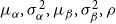
where \begin{align*} p(\mathbf{Z}, \alpha \mid \boldsymbol{\mathrm{Y}}) &\propto p(\boldsymbol{\mathrm{Y}} \mid \alpha , \mathbf{Z}) \cdot \prod _{i} p(\mathbf{z}_i) \cdot p(\alpha ) \\ &\propto \prod _{i \lt j} p_{i,j}^{y_{i,j}} (1 - p_{i,j})^{1-y_{i,j}} \cdot \exp \left (-\frac {1}{2\sigma _{z}^2}\textstyle \sum _{i}\|\mathbf{z}_{i}\|^2\right ) \cdot \exp \left (-\frac {1}{2\sigma _{\alpha }^2}(\alpha -\mu _\alpha )^2\right )\!, \end{align*}
$\mu _\alpha ,\sigma _\alpha ^2$
, and
$\sigma ^2_z$
are known hyperparameters.
\begin{align*} p(\mathbf{Z}, \alpha \mid \boldsymbol{\mathrm{Y}}) &\propto p(\boldsymbol{\mathrm{Y}} \mid \alpha , \mathbf{Z}) \cdot \prod _{i} p(\mathbf{z}_i) \cdot p(\alpha ) \\ &\propto \prod _{i \lt j} p_{i,j}^{y_{i,j}} (1 - p_{i,j})^{1-y_{i,j}} \cdot \exp \left (-\frac {1}{2\sigma _{z}^2}\textstyle \sum _{i}\|\mathbf{z}_{i}\|^2\right ) \cdot \exp \left (-\frac {1}{2\sigma _{\alpha }^2}(\alpha -\mu _\alpha )^2\right )\!, \end{align*}
$\mu _\alpha ,\sigma _\alpha ^2$
, and
$\sigma ^2_z$
are known hyperparameters.
-
• Spherical latent distance model:
where
\begin{align*} p(\alpha , \beta , \mathbf{Z} \mid \boldsymbol{\mathrm{Y}}) &\propto p(\boldsymbol{\mathrm{Y}} \mid \alpha ,\beta ,\mathbf{Z}) \cdot \prod _{i} p(\mathbf{z}_i) \cdot p(\alpha , \beta ) \\ &= \prod _{i \lt j} p_{i,j}^{y_{i,j}} (1 - p_{i,j})^{1-y_{i,j}} \cdot \exp \left (-\frac {1}{2(1-\rho ^2)} Q(\alpha , \beta ) \right )\!, \end{align*}
$\mu _\alpha ,\sigma _\alpha ^2,\mu _\beta ,\sigma _\beta ^2,\rho$
, and
$\sigma ^2_z$
are known hyperparameters, and
\begin{equation*} Q(\alpha , \beta ) = \frac {(\alpha - \mu _\alpha )^2}{\sigma _\alpha ^2} - \frac {2\rho \, \alpha (\beta - \mu _\beta )}{\sigma _\alpha \sigma _\beta } + \frac {(\beta - \mu _\beta )^2}{\sigma _\beta ^2}. \end{equation*}




Posterior summaries such as the posterior mean $(\theta ^{\text{PM}}, \mathbf{Z}^{\text{PM}}) = \textsf {E}(\theta , \mathbf{Z} \mid \mathbf{Y})$
and the maximum a posteriori
$(\theta ^{\text{PM}}, \mathbf{Z}^{\text{PM}}) = \textsf {E}(\theta , \mathbf{Z} \mid \mathbf{Y})$
and the maximum a posteriori $(\theta ^{\text{MAP}}, \mathbf{Z}^{\text{MAP}}) = \arg \max p(\theta , \mathbf{Z} \mid \mathbf{Y})$
provide interpretable point estimates of the model parameters, capturing the central tendency of the latent structure, while credible regions derived from the posterior distribution quantify the uncertainty associated with these estimates.
$(\theta ^{\text{MAP}}, \mathbf{Z}^{\text{MAP}}) = \arg \max p(\theta , \mathbf{Z} \mid \mathbf{Y})$
provide interpretable point estimates of the model parameters, capturing the central tendency of the latent structure, while credible regions derived from the posterior distribution quantify the uncertainty associated with these estimates.
3.2.1 Sampling algorithms
The posterior distributions of the latent space models described here are high-dimensional and analytically intractable. To address this challenge, we approximate the posterior using MCMC methods (e.g., Gamerman and Lopes, Reference Gamerman and Lopes2006), specifically the Metropolis–Hastings (MH) algorithm (e.g., Albert et al., Reference Albert2009), the Hamiltonian Monte Carlo (HMC) algorithm (e.g., Gelman et al., Reference Gelman, Carlin, Stern, Dunson, Vehtari and Rubin2013a), and the Spherical HMC algorithm (e.g., Yu, Reference Yu2020), which are developed throughout this section. These approaches provide the flexibility to design geometry-aware proposal distributions tailored to both Euclidean and spherical latent spaces.
Metropolis–Hastings algorithm
Let $\mathbf{Z}$
denote the matrix of latent positions, and let
$\mathbf{Z}$
denote the matrix of latent positions, and let $\theta$
represent the global model parameters (
$\theta$
represent the global model parameters ( $\alpha$
in the Euclidean case, and both
$\alpha$
in the Euclidean case, and both $\alpha$
and
$\alpha$
and $\beta$
in the spherical formulation). The unnormalized log-posterior density is
$\beta$
in the spherical formulation). The unnormalized log-posterior density is
 \begin{equation*} \psi (\theta , \mathbf{Z}) = \log p(\mathbf{Y} \mid \theta , \mathbf{Z}) + \log p(\mathbf{Z}) + \log p(\theta ), \end{equation*}
which is the sum of the log-likelihood and the log-prior densities for the latent positions and the model parameters. The Markov chain is initialized by sampling $\theta$
and
$\theta$
and $\mathbf{Z}$
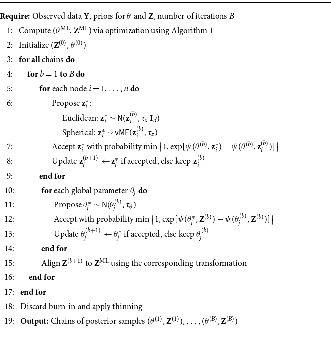
from their prior distributions, although maximum likelihood estimates may also serve as effective starting values. We employ a Metropolis algorithm with symmetric proposal distributions, adjusting their variances during the burn-in phase to achieve target acceptance rates, typically between 30% and 50%. The joint posterior is explored by alternately updating
$\mathbf{Z}$
from their prior distributions, although maximum likelihood estimates may also serve as effective starting values. We employ a Metropolis algorithm with symmetric proposal distributions, adjusting their variances during the burn-in phase to achieve target acceptance rates, typically between 30% and 50%. The joint posterior is explored by alternately updating $\theta$
and
$\theta$
and $\mathbf{Z}$
via Metropolis steps, with minor procedural differences between the Euclidean and spherical formulations.
$\mathbf{Z}$
via Metropolis steps, with minor procedural differences between the Euclidean and spherical formulations.
Latent positions are updated sequentially by proposing a candidate $\mathbf{z}_i^\ast$
, for each
$\mathbf{z}_i^\ast$
, for each $i = 1, \ldots , n$
, one at a time. In the Euclidean case, proposals are drawn from a multivariate Normal distribution centered at the current position,
$i = 1, \ldots , n$
, one at a time. In the Euclidean case, proposals are drawn from a multivariate Normal distribution centered at the current position,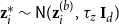 $\mathbf{z}_i^\ast \sim \textsf {N}(\mathbf{z}_i^{(b)}, \tau _{z}\, \mathbf{I}_d)$
, where
$\mathbf{z}_i^\ast \sim \textsf {N}(\mathbf{z}_i^{(b)}, \tau _{z}\, \mathbf{I}_d)$
, where $\tau _{z}$
is a tuning parameter. In the spherical case, following Wood (Reference Wood1994) and Mardia and Jupp (Reference Mardia and Jupp2000), proposals are drawn from a von Mises–Fisher distribution with mean direction equal to the current position,
$\tau _{z}$
is a tuning parameter. In the spherical case, following Wood (Reference Wood1994) and Mardia and Jupp (Reference Mardia and Jupp2000), proposals are drawn from a von Mises–Fisher distribution with mean direction equal to the current position,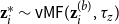 $\mathbf{z}_i^\ast \sim \textsf {vMF}(\mathbf{z}_i^{(b)}, \tau _{z})$
. The proposed value is accepted with probability
$\mathbf{z}_i^\ast \sim \textsf {vMF}(\mathbf{z}_i^{(b)}, \tau _{z})$
. The proposed value is accepted with probability $\min \big \{ 1, {\exp} {[ \psi (\theta ^{(b)}, \mathbf{z}_i^\ast ) - \psi (\theta ^{(b)}, \mathbf{z}_i^{(b)}) ] }\big \}$
, where the log-posterior is evaluated holding all latent positions fixed except for node
$\min \big \{ 1, {\exp} {[ \psi (\theta ^{(b)}, \mathbf{z}_i^\ast ) - \psi (\theta ^{(b)}, \mathbf{z}_i^{(b)}) ] }\big \}$
, where the log-posterior is evaluated holding all latent positions fixed except for node $i$
. If accepted, the proposed value becomes the new state
$i$
. If accepted, the proposed value becomes the new state $\mathbf{z}_i^{(b+1)} = \mathbf{z}_i^\ast$
; otherwise, the position remains unchanged.
$\mathbf{z}_i^{(b+1)} = \mathbf{z}_i^\ast$
; otherwise, the position remains unchanged.
The global parameters are updated sequentially. For each parameter, a candidate $\theta ^\ast$
is proposed from a Normal distribution centered at the current value,
$\theta ^\ast$
is proposed from a Normal distribution centered at the current value, $\theta ^\ast \sim \textsf {N}(\theta ^{(b)}, \tau _\theta )$
, where
$\theta ^\ast \sim \textsf {N}(\theta ^{(b)}, \tau _\theta )$
, where $\tau _{\theta }$
is once again a tuning parameter. The acceptance probability is computed as
$\tau _{\theta }$
is once again a tuning parameter. The acceptance probability is computed as $\min \{1, \exp [ \psi (\theta ^\ast , \mathbf{Z}^{(b)}) - \psi (\theta ^{(b)}, \mathbf{Z}^{(b)}) ] \}$
, analogous to the latent position updates, and the proposed value is accepted or rejected accordingly.
$\min \{1, \exp [ \psi (\theta ^\ast , \mathbf{Z}^{(b)}) - \psi (\theta ^{(b)}, \mathbf{Z}^{(b)}) ] \}$
, analogous to the latent position updates, and the proposed value is accepted or rejected accordingly.
Finally, to account for isometric invariance in the latent space, each sampled configuration $\mathbf{Z}^{(b+1)}$
is aligned to the maximum likelihood estimate
$\mathbf{Z}^{(b+1)}$
is aligned to the maximum likelihood estimate $\mathbf{Z}^{\text{ML}}$
using a Procrustes transformation (e.g., Borg and Groenen, Reference Borg and Groenen2005). In the Euclidean case, the transformation
$\mathbf{Z}^{\text{ML}}$
using a Procrustes transformation (e.g., Borg and Groenen, Reference Borg and Groenen2005). In the Euclidean case, the transformation $\mathbf{T}$
minimizes the trace of the squared distances:
$\mathbf{T}$
minimizes the trace of the squared distances:
 \begin{equation*} \tilde {\mathbf{Z}}^{(b+1)} = \underset {\mathbf{T}}{\arg \min } \ \text{tr} \Big [ \big (\mathbf{Z}^{\text{ML}} - \mathbf{T}\,\mathbf{Z}^{(b+1)}\big)^{\top} \big (\mathbf{Z}^{\text{ML}} - \mathbf{T}\,\mathbf{Z}^{(b+1)}\big ) \Big ]. \end{equation*}
In the spherical case, the alignment is performed via an orthogonal transformation $\mathbf{T}$
that minimizes the Frobenius norm (e.g., Golub and Van Loan, Reference Golub and Van Loan2013):
$\mathbf{T}$
that minimizes the Frobenius norm (e.g., Golub and Van Loan, Reference Golub and Van Loan2013):
 \begin{equation*} \tilde {\mathbf{Z}}^{(b+1)} = \underset {\mathbf{T}}{\arg \min } \ \big \| \mathbf{Z}^{\text{ML}} - \mathbf{T}\,\mathbf{Z}^{(b+1)} \big \|_F, \end{equation*}
with $\mathbf{T}^{\top} \mathbf{T} = \mathbf{I}_n$
.
$\mathbf{T}^{\top} \mathbf{T} = \mathbf{I}_n$
.
After discarding an initial burn-in period and applying thinning when necessary, the retained posterior samples can be used to compute summary statistics of interest, including point estimates and marginal credible intervals for all model parameters, including latent positions. Convergence and mixing are evaluated using standard MCMC diagnostics across multiple chains, such as the effective sample size (ESS) and the potential scale reduction factor $\hat {R}$
. The complete estimation procedure is outlined in Algorithm 2.
$\hat {R}$
. The complete estimation procedure is outlined in Algorithm 2.
Metropolis–Hastings algorithm for latent space models
Hamiltonian Monte Carlo algorithm
Alongside the Metropolis–Hastings algorithm we consider two advanced sampling methods, HMC and GHMC. These approaches exploit gradient information and the underlying geometric structure to explore the posterior distribution more efficiently, particularly in high dimensional or curved latent spaces. In our latent space models we use HMC to update unconstrained global parameters and Euclidean latent coordinates, and we use GHMC for latent positions constrained to lie on the hypersphere. Each Hamiltonian update targets the full conditional distribution of either the parameter vector $\boldsymbol{\theta }$
or a single latent position
$\boldsymbol{\theta }$
or a single latent position $\mathbf z_i$
, with all remaining components held fixed, which leads to an MCMC scheme where Hamiltonian steps are applied one at a time to the components of
$\mathbf z_i$
, with all remaining components held fixed, which leads to an MCMC scheme where Hamiltonian steps are applied one at a time to the components of $(\boldsymbol{\theta },\mathbf Z)$
. While these updates can achieve higher sampling efficiency by accounting for the curvature of the full conditional distributions, they are computationally more demanding because they require gradient evaluations and auxiliary momentum variables. For clarity we first recall the generic HMC and GHMC schemes in abstract form before describing their implementation for the latent space models.
$(\boldsymbol{\theta },\mathbf Z)$
. While these updates can achieve higher sampling efficiency by accounting for the curvature of the full conditional distributions, they are computationally more demanding because they require gradient evaluations and auxiliary momentum variables. For clarity we first recall the generic HMC and GHMC schemes in abstract form before describing their implementation for the latent space models.
The HMC algorithm expands the parameter space by introducing an auxiliary momentum variable $\mathbf{p}$
, which enables the use of Hamiltonian dynamics to generate proposals (Neal, Reference Neal, Brooks, Gelman, Jones and Meng2011). For a target unnormalized density
$\mathbf{p}$
, which enables the use of Hamiltonian dynamics to generate proposals (Neal, Reference Neal, Brooks, Gelman, Jones and Meng2011). For a target unnormalized density $f(\mathbf{x})$
, the Hamiltonian is given by
$f(\mathbf{x})$
, the Hamiltonian is given by
 \begin{equation*} \mathrm{H}(\mathbf{x}, \mathbf{p}) = \mathrm{U}(\mathbf{x}) + \frac {1}{2} \mathbf{p}^{\top} \mathbf{M}^{-1} \mathbf{p}, \end{equation*}
where $\mathrm{U}(\mathbf{x}) = -\log f(\mathbf{x})$
represents the potential energy associated with the unnormalized log-density
$\mathrm{U}(\mathbf{x}) = -\log f(\mathbf{x})$
represents the potential energy associated with the unnormalized log-density $\log f(\mathbf{x})$
, and
$\log f(\mathbf{x})$
, and $\mathbf{M}$
is a symmetric positive-definite mass matrix, often chosen as the identity for simplicity.
$\mathbf{M}$
is a symmetric positive-definite mass matrix, often chosen as the identity for simplicity.
The dynamics are determined by Hamilton’s equations and are numerically integrated via the leapfrog method using a fixed step size $\epsilon$
and a predetermined number of steps
$\epsilon$
and a predetermined number of steps $L$
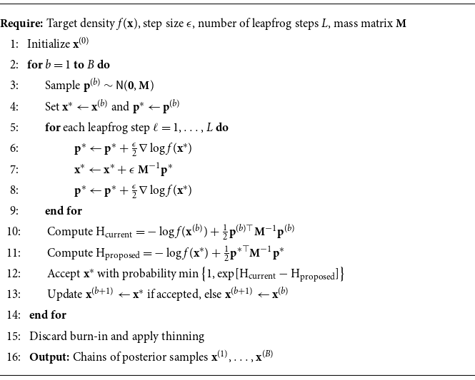
(Sanz-Serna and Calvo, Reference Sanz-Serna and Calvo2018). These algorithmic parameters are tuned during execution to balance computational efficiency and acceptance probability, which typically lies between 60% and 70%. A proposal state is obtained by simulating the Hamiltonian dynamics forward in time, after which it is accepted or rejected according to a Metropolis rule that preserves detailed balance. This approach enables the sampler to perform large, gradient-informed moves across the posterior space, offering substantial efficiency gains over regular random-walk proposals (Neal, Reference Neal, Brooks, Gelman, Jones and Meng2011). Algorithm 3 outlines the HMC procedure for sampling from a general target distribution. For the Euclidean latent space model we apply the generic HMC step to the full conditional of each latent coordinate. In the notation of Algorithm 3 we take
$L$
(Sanz-Serna and Calvo, Reference Sanz-Serna and Calvo2018). These algorithmic parameters are tuned during execution to balance computational efficiency and acceptance probability, which typically lies between 60% and 70%. A proposal state is obtained by simulating the Hamiltonian dynamics forward in time, after which it is accepted or rejected according to a Metropolis rule that preserves detailed balance. This approach enables the sampler to perform large, gradient-informed moves across the posterior space, offering substantial efficiency gains over regular random-walk proposals (Neal, Reference Neal, Brooks, Gelman, Jones and Meng2011). Algorithm 3 outlines the HMC procedure for sampling from a general target distribution. For the Euclidean latent space model we apply the generic HMC step to the full conditional of each latent coordinate. In the notation of Algorithm 3 we take $x = \mathbf z_i$
and
$x = \mathbf z_i$
and $f(x) \propto \exp \{\psi (\theta ,\mathbf Z)\}$
with all components except
$f(x) \propto \exp \{\psi (\theta ,\mathbf Z)\}$
with all components except $\mathbf z_i$
fixed, and we use the same scheme for blocks of unconstrained global parameters when convenient.
$\mathbf z_i$
fixed, and we use the same scheme for blocks of unconstrained global parameters when convenient.
Hamiltonian Monte Carlo algorithm
Spherical Hamiltonian Monte Carlo algorithm
Standard Hamiltonian Monte Carlo (HMC) performs effectively in flat Euclidean spaces, but it can be restrictive when the posterior distribution is supported on a curved manifold. To handle parameters constrained to lie on the hypersphere, in particular the latent positions $\mathbf z_i \in \mathbb S^{d-1}$
in the spherical model, we adopt Geodesic Hamiltonian Monte Carlo (GHMC), an extension of HMC designed for embedded Riemannian manifolds such as spheres or Stiefel manifolds and inspired by the Riemannian Manifold HMC framework of Girolami and Calderhead (Reference Girolami and Calderhead2011). In the spherical latent space model, however, the latent positions are constrained to lie on the hypersphere
$\mathbf z_i \in \mathbb S^{d-1}$
in the spherical model, we adopt Geodesic Hamiltonian Monte Carlo (GHMC), an extension of HMC designed for embedded Riemannian manifolds such as spheres or Stiefel manifolds and inspired by the Riemannian Manifold HMC framework of Girolami and Calderhead (Reference Girolami and Calderhead2011). In the spherical latent space model, however, the latent positions are constrained to lie on the hypersphere $\mathbb{S}^{d-1}$
. Standard HMC algorithms are formulated for unconstrained Euclidean parameter spaces, and a direct application of a generic Euclidean HMC update would generate proposals outside the manifold. Enforcing the spherical constraint would then require projection steps that disrupt the symplectic structure of the Hamiltonian dynamics and can degrade mixing. In particular, Stan’s default No-U-Turn Sampler (NUTS) implementation assumes unconstrained Euclidean parameters and would require nontrivial reparameterization together with Jacobian adjustments to accommodate spherical constraints. By contrast, the GHMC algorithm operates directly on the embedded sphere, preserving the manifold constraint intrinsically and evolving proposals along exact geodesic flows without the need for reparameterization.
$\mathbb{S}^{d-1}$
. Standard HMC algorithms are formulated for unconstrained Euclidean parameter spaces, and a direct application of a generic Euclidean HMC update would generate proposals outside the manifold. Enforcing the spherical constraint would then require projection steps that disrupt the symplectic structure of the Hamiltonian dynamics and can degrade mixing. In particular, Stan’s default No-U-Turn Sampler (NUTS) implementation assumes unconstrained Euclidean parameters and would require nontrivial reparameterization together with Jacobian adjustments to accommodate spherical constraints. By contrast, the GHMC algorithm operates directly on the embedded sphere, preserving the manifold constraint intrinsically and evolving proposals along exact geodesic flows without the need for reparameterization.
Unlike RMHMC, which requires computing local metric tensors and numerically integrating the geodesic equations, GHMC exploits the manifold’s known geodesic structure to evolve trajectories exactly along curvature aware paths. In this setting, the target density is expressed with respect to the Hausdorff measure (Federer, Reference Federer2014), leading to the modified Hamiltonian
 \begin{equation*} \mathrm{H}_{\mathcal{H}}(\mathbf{x}, \mathbf{p}) = -\log f_{\mathcal{H}}(\mathbf{x}) + \frac {1}{2} \mathbf{p}^{\top} \mathrm{G}(\mathbf{x})^{-1} \mathbf{p}, \end{equation*}
where $\mathrm{G}(\mathbf{x})$
is the intrinsic metric tensor of the manifold and
$\mathrm{G}(\mathbf{x})$
is the intrinsic metric tensor of the manifold and $f_{\mathcal{H}}(\mathbf{x})$
is the target density adjusted by the Riemannian volume element
$f_{\mathcal{H}}(\mathbf{x})$
is the target density adjusted by the Riemannian volume element $\sqrt {|\mathrm{G}(\mathbf{x})|}$
(Byrne and Girolami, Reference Byrne and Girolami2013). In our application each GHMC update targets the full conditional distribution of a single latent position
$\sqrt {|\mathrm{G}(\mathbf{x})|}$
(Byrne and Girolami, Reference Byrne and Girolami2013). In our application each GHMC update targets the full conditional distribution of a single latent position $\mathbf z_i$
on
$\mathbf z_i$
on $\mathbb S^{d-1}$
and the proposal follows a geodesic flow on the sphere.
$\mathbb S^{d-1}$
and the proposal follows a geodesic flow on the sphere.
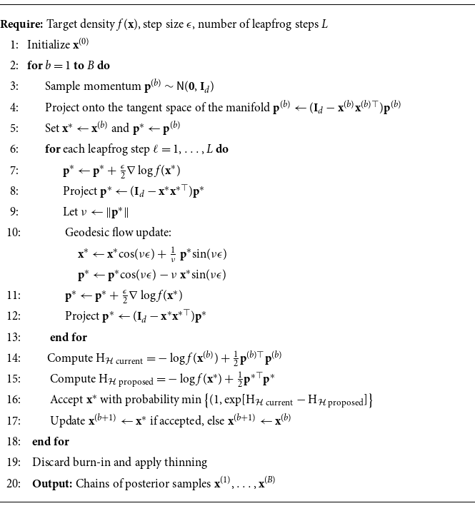
GHMC alternates between exact geodesic updates of position and velocity (the kinetic flow) and momentum adjustments driven by the gradient of the log-density (the potential flow). On the hypersphere, these geodesic updates admit closed-form solutions involving trigonometric functions of the angular velocity, enabling efficient and numerically stable integration. After a predetermined number of integration steps, a Metropolis acceptance step ensures that the resulting Markov chain targets the correct posterior distribution. To preserve the validity of the dynamics, the momentum is projected onto the tangent space of the manifold after each update. By explicitly exploiting the manifold’s geometric structure, GHMC retains the principal advantages of HMC, such as long-distance proposals and reduced random-walk behavior, while remaining well-defined on curved latent spaces. In contrast to RMHMC, which requires computing and differentiating a position-dependent metric tensor at each iteration (Girolami and Calderhead, Reference Girolami and Calderhead2011), GHMC avoids these computational burdens by relying on analytically tractable geodesic flows, making it a scalable alternative for manifold-constrained models (Yu, Reference Yu2020). Algorithm 4 presents the GHMC procedure for sampling from an arbitrary density supported on a spherical manifold. This algorithm summarizes one update for a latent position in the spherical model. In this case we set $x = \mathbf z_i$
and
$x = \mathbf z_i$
and $f(x) \propto \exp \{\psi (\boldsymbol{\theta },\mathbf Z)\}$
restricted to
$f(x) \propto \exp \{\psi (\boldsymbol{\theta },\mathbf Z)\}$
restricted to $\mathbb S^{d-1}$
, and the projection and geodesic moves act directly on the latent coordinate
$\mathbb S^{d-1}$
, and the projection and geodesic moves act directly on the latent coordinate $\mathbf z_i$
.
$\mathbf z_i$
.
Spherical Hamiltonian Monte Carlo algorithm
Hamiltonian-based algorithms must be adapted to latent space network models by tuning hyperparameters, updating parameters sequentially to improve acceptance rates, and respecting the geometry of the latent space. Convergence diagnostics ensure adequate posterior exploration and reliability of inferences, while multimodality and identifiability issues require running multiple chains from diverse initializations and checking the consistency of marginal posteriors. Geometric constraints add further complexity, necessitating careful algorithmic design to balance exploration efficiency, numerical stability, and convergence guarantees.
For readers interested in a concrete illustration of these algorithms in a controlled setting, Appendix A presents a detailed comparison of Metropolis–Hastings, HMC, and GHMC for sampling from the bivariate Rosenbrock density. This target has strong curvature and non quadratic contours, and is a standard benchmark for assessing the ability of MCMC schemes to explore narrow, curved posterior regions. The example reports ESSs, acceptance rates, and trace plots, which help to visualize the efficiency gains of Hamiltonian based methods when needed.
4. Illustration: Florentine families
We illustrate the latent space models using two benchmark social science networks originally analyzed by Hoff et al. (Reference Hoff, Raftery and Handcock2002). The main text presents results for the Florentine families data, while the supplementary material reports findings for the monks data. These datasets differ in scale, domain, and type of interaction, offering a diverse testbed for assessing model behavior and interpretability. For each, we fit the proposed model to the observed relational data and analyze the latent structure, inference results, and model fit via posterior summaries and predictive checks. The examples include a historical marriage network among Florentine families and interpersonal ties among monks in a monastery.
In historical social network analysis, relationships between influential families reveal power dynamics, alliances, and social structures. A notable example is the study by Padgett and Ansell (Reference Padgett and Ansell1993), which examines marriage and business ties among 16 prominent Florentine families in the 15th century, drawing on historical accounts that document the socio-political landscape of Renaissance Florence.
Visualization of the marriage network among Florentine families.
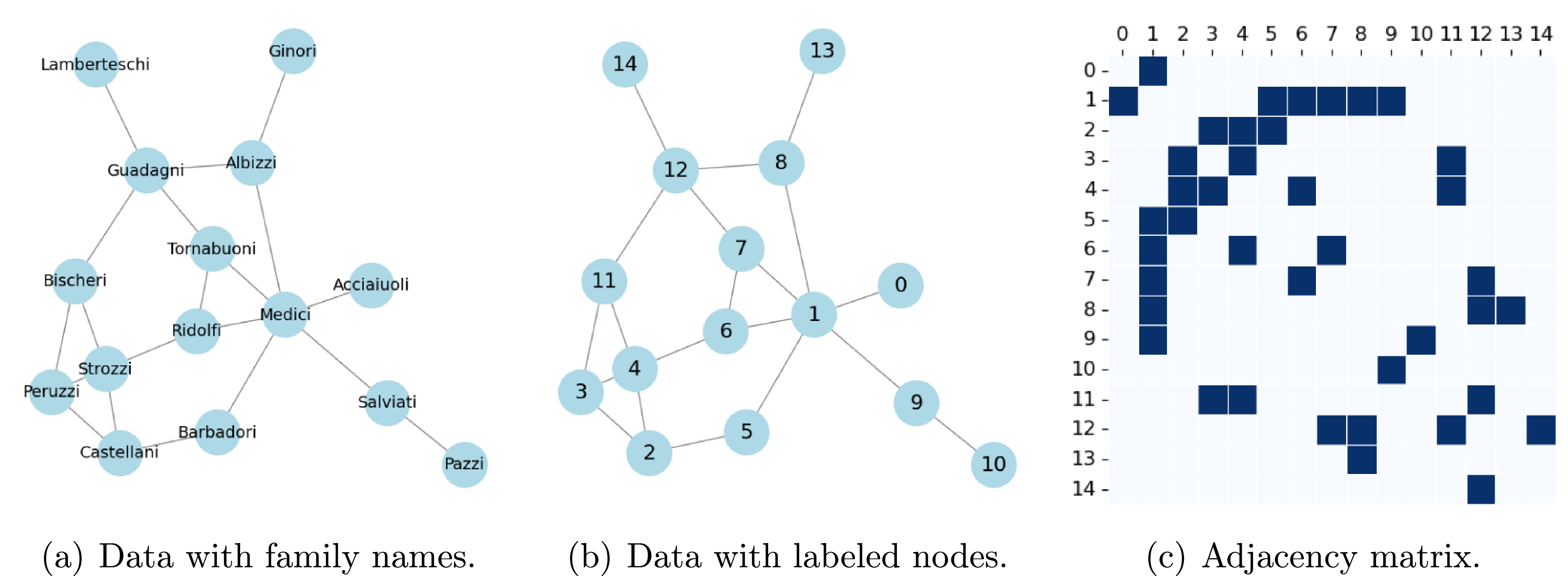
This model focuses on marriage relations between these families, where a tie indicates at least one marriage between them. The network is undirected. One of the 16 families, having no marriage ties, was excluded to avoid infinite distances in maximum likelihood estimation and large finite distances in a Bayesian framework. Modeling these relations with network analysis techniques reveals the structural properties of the Florentine elite and their strategic matrimonial alliances, offering insights into how marriage shaped political and economic power during the Renaissance. Figure 2 shows the network, its relabeling, and the sociomatrix.
We fit the models in $\mathbb{R}^1$
,
$\mathbb{R}^1$
, $\mathbb{R}^2$
,
$\mathbb{R}^2$
, $\mathbb{R}^3$
,
$\mathbb{R}^3$
, $\mathbb{S}^1$
, and
$\mathbb{S}^1$
, and $\mathbb{S}^2$
using Algorithms 2, 3, and 4, with hyperparameters
$\mathbb{S}^2$
using Algorithms 2, 3, and 4, with hyperparameters $\sigma _{\mathbf{z}} = 5.0$
and
$\sigma _{\mathbf{z}} = 5.0$
and $\sigma _\alpha = 5.0$
for the Euclidean model, and
$\sigma _\alpha = 5.0$
for the Euclidean model, and $\rho = -0.5$
,
$\rho = -0.5$
, $\mu _\alpha = 0.0$
,
$\mu _\alpha = 0.0$
, $\sigma _\alpha = 1.0$
,
$\sigma _\alpha = 1.0$
, $\mu _\beta = 10.0$
, and
$\mu _\beta = 10.0$
, and $\sigma _{\beta } = 5.0$
for the spherical model. Hyperparameters were selected via sensitivity analysis to optimize information and predictive criteria (supplementary material). While Hamiltonian dynamics methods (Algorithms 3 and 4) yield higher ESS per iteration, they require gradient evaluations that increase computation time and may introduce numerical instabilities.
$\sigma _{\beta } = 5.0$
for the spherical model. Hyperparameters were selected via sensitivity analysis to optimize information and predictive criteria (supplementary material). While Hamiltonian dynamics methods (Algorithms 3 and 4) yield higher ESS per iteration, they require gradient evaluations that increase computation time and may introduce numerical instabilities.
To examine this tradeoff directly within the Florentine network model, we estimated both the Euclidean model in $\mathbb{R}^3$
and the spherical model in
$\mathbb{R}^3$
and the spherical model in $\mathbb{S}^2$
using Metropolis–Hastings (MH), Hamiltonian Monte Carlo (HMC), and Geodesic Hamiltonian Monte Carlo (GHMC). For the
$\mathbb{S}^2$
using Metropolis–Hastings (MH), Hamiltonian Monte Carlo (HMC), and Geodesic Hamiltonian Monte Carlo (GHMC). For the $\mathbb{R}^3$
model, latent positions were initialized from anisotropic Gaussian distributions with
$\mathbb{R}^3$
model, latent positions were initialized from anisotropic Gaussian distributions with $\alpha ^{(0)}=0$
. We ran two chains of 10,000 posterior samples after a burn-in of 10,000 iterations with thinning of 50. Proposal scales were
$\alpha ^{(0)}=0$
. We ran two chains of 10,000 posterior samples after a burn-in of 10,000 iterations with thinning of 50. Proposal scales were $\sigma _{q,\mathbf{Z}}=\sigma _{q,\alpha }=1.0$
, and HMC step sizes were
$\sigma _{q,\mathbf{Z}}=\sigma _{q,\alpha }=1.0$
, and HMC step sizes were $\epsilon _{\mathbf{Z}}=\epsilon _{\alpha }=0.1$
with
$\epsilon _{\mathbf{Z}}=\epsilon _{\alpha }=0.1$
with $L = \lfloor \epsilon ^{-1} \rfloor$
. For the
$L = \lfloor \epsilon ^{-1} \rfloor$
. For the $\mathbb{S}^2$
model, latent positions were initialized from a von Mises–Fisher distribution centered at
$\mathbb{S}^2$
model, latent positions were initialized from a von Mises–Fisher distribution centered at $(0,0,1)$
with concentration
$(0,0,1)$
with concentration $\kappa =0$
, ensuring uniform initialization on the sphere. We used analogous chain lengths and tuning strategies, with Geodesic HMC step sizes
$\kappa =0$
, ensuring uniform initialization on the sphere. We used analogous chain lengths and tuning strategies, with Geodesic HMC step sizes $\epsilon _{\mathbf{Z}}=\epsilon _{\alpha }=\epsilon _{\beta }=0.1$
and trajectory lengths defined similarly. During burn-in, proposal scales were tuned to achieve acceptance rates between 30% and 50% for MH and between 60% and 80% for HMC and GHMC.
$\epsilon _{\mathbf{Z}}=\epsilon _{\alpha }=\epsilon _{\beta }=0.1$
and trajectory lengths defined similarly. During burn-in, proposal scales were tuned to achieve acceptance rates between 30% and 50% for MH and between 60% and 80% for HMC and GHMC.
Likelihood traces for latent position model parameters in $\mathbb{R}^3$
and
$\mathbb{R}^3$
and $\mathbb{S}^2$
for the Florentine families example, obtained using Metropolis and Hamiltonian based sampling algorithms.
$\mathbb{S}^2$
for the Florentine families example, obtained using Metropolis and Hamiltonian based sampling algorithms.
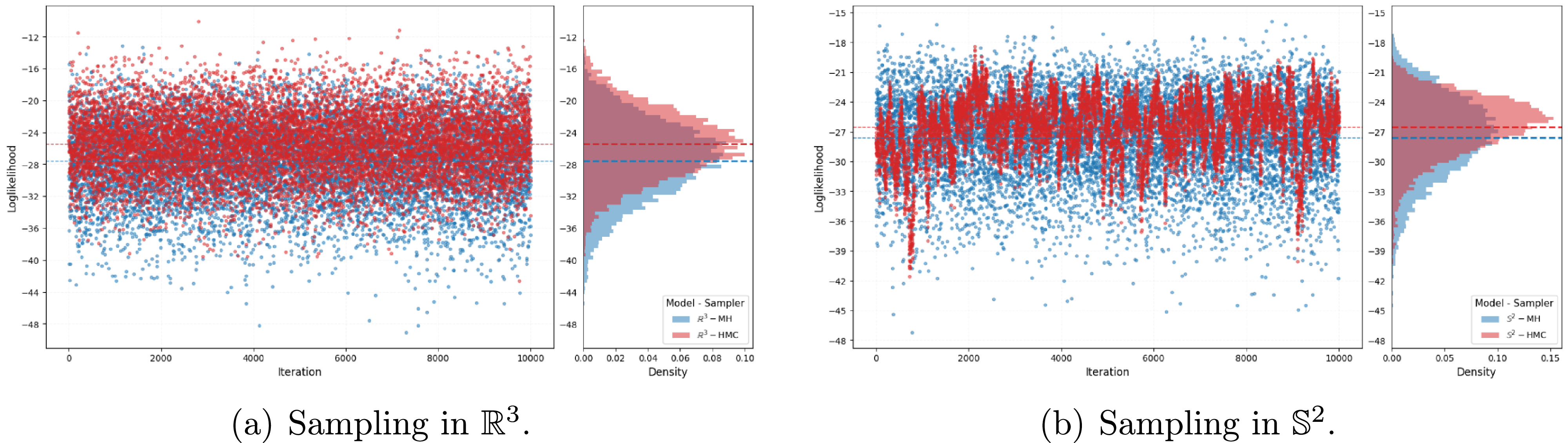
Figure 3 shows the likelihood traces for each sampler, and Table 1 summarizes convergence diagnostics, ESS), and computational cost. Across geometries, Hamiltonian-based samplers generally achieve higher minimum relative ESS than MH, indicating more efficient posterior exploration per iteration, at the expense of increased computational cost due to gradient evaluations. However, the behavior of GHMC differs from standard HMC. In the spherical setting, GHMC exhibits stronger autocorrelation and slower mixing in the trace plots, along with a tendency to explore a narrower region of the posterior distribution. This pattern is consistent with the interaction between manifold curvature and the numerical integration of the geodesic flow, which can increase sensitivity to tuning parameters. Despite these differences in mixing behavior, posterior summaries remain qualitatively consistent across samplers, indicating that the choice of algorithm primarily affects computational efficiency and sampling dynamics rather than substantive inference.
Comparison of MH, HMC, and GHMC for the Florentine families latent space model in $\mathbb{R}^3$
and
$\mathbb{R}^3$
and $\mathbb{S}^2$
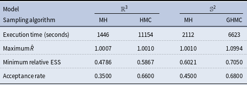
Given this qualitative agreement across samplers, and in order to maintain computational comparability across all geometric specifications and dimensions, we use the MH algorithm for the reported results. Convergence was confirmed through standard diagnostics (Gelman et al., Reference Gelman, Carlin, Stern, Dunson, Vehtari and Rubin2013a). We then assess model fit and performance by inspecting log-likelihood trajectories from MH sampling (Figure 4). All models exhibit good convergence, with the Euclidean model in $\mathbb{R}^3$
achieving the highest likelihood, followed by the spherical model in
$\mathbb{R}^3$
achieving the highest likelihood, followed by the spherical model in $\mathbb{S}^2$
.
$\mathbb{S}^2$
.
Log-likelihood trajectories for all models obtained during MCMC sampling.
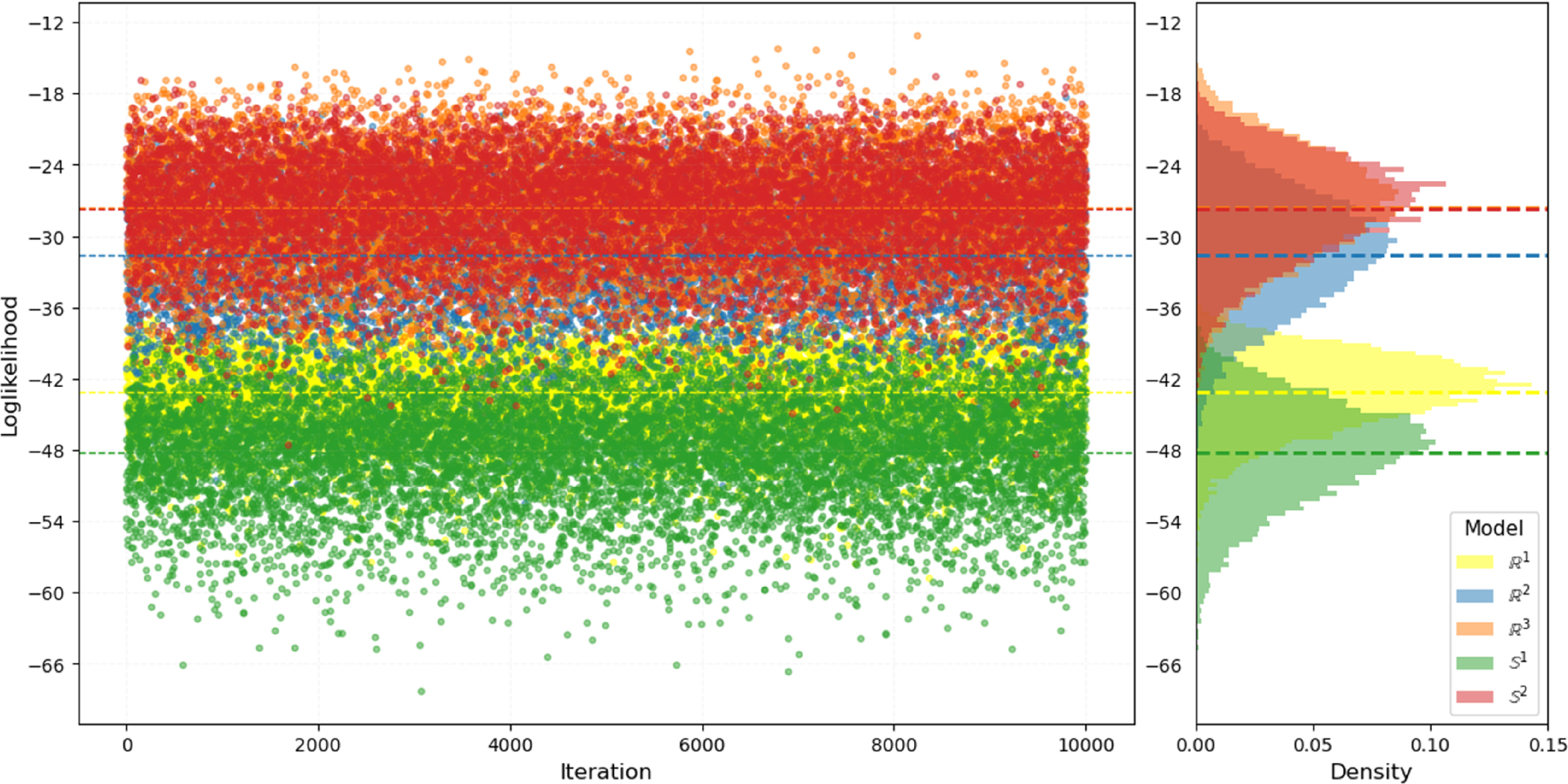
Table 2 reports the Watanabe–Akaike information criteria (e.g., Watanabe, Reference Watanabe2013, Gelman et al., Reference Gelman, Hwang and Vehtari2014) for each model. Spherical models achieve log-likelihood values close to their Euclidean counterparts, indicating comparable ability to capture network structure despite geometric constraints that reduce the effective degrees of freedom: for $n$
nodes and dimension
$n$
nodes and dimension $d$
, a model in
$d$
, a model in $\mathbb{R}^d$
has
$\mathbb{R}^d$
has $n d + 1$
degrees of freedom, whereas a model in
$n d + 1$
degrees of freedom, whereas a model in $\mathbb{S}^{d-1}$
has
$\mathbb{S}^{d-1}$
has $n (d - 1) + 2$
due to constraints on latent positions. WAIC favors the Euclidean model in
$n (d - 1) + 2$
due to constraints on latent positions. WAIC favors the Euclidean model in $\mathbb{R}^3$
, with the one in
$\mathbb{R}^3$
, with the one in $\mathbb{R}^2$
close behind, while the model in
$\mathbb{R}^2$
close behind, while the model in $\mathbb{S}^2$
attains values close to the best Euclidean specifications and the model in
$\mathbb{S}^2$
attains values close to the best Euclidean specifications and the model in $\mathbb{S}^1$
performs noticeably worse, reflecting the limited flexibility of a circle. Overall, the spherical models remain competitive in terms of fit, with
$\mathbb{S}^1$
performs noticeably worse, reflecting the limited flexibility of a circle. Overall, the spherical models remain competitive in terms of fit, with $\mathbb{S}^2$
in particular combining parsimony, geometric interpretability, and good likelihood based performance.
$\mathbb{S}^2$
in particular combining parsimony, geometric interpretability, and good likelihood based performance.
Model comparison metrics for each latent space specification. The mean log-likelihood is averaged over posterior samples, while ML, MAP, and CM denote the log-likelihood evaluated at the maximum likelihood estimate, the maximum a posteriori estimate, and the posterior mean, respectively
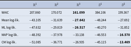
Latent space representations for $\mathbb{R}^1$
and
$\mathbb{R}^1$
and $\mathbb{S}^1$
models, showing each node’s posterior distribution and mean position, with edges indicating ties from the original network.
$\mathbb{S}^1$
models, showing each node’s posterior distribution and mean position, with edges indicating ties from the original network.
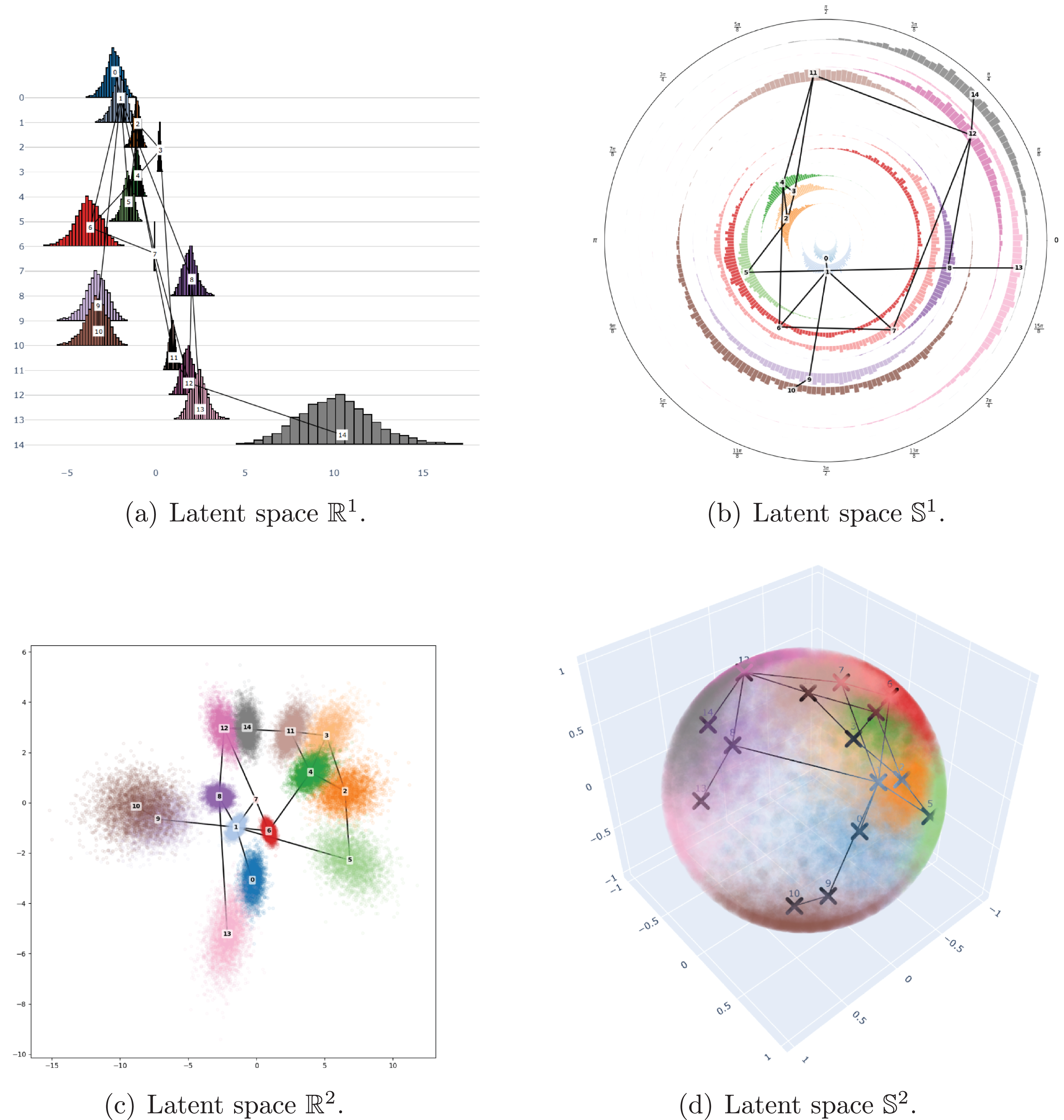
Figure 5 shows the estimated node positions for the models in $\mathbb{R}^1$
and
$\mathbb{R}^1$
and $\mathbb{S}^2$
. Both Euclidean and spherical embeddings preserve much of the original graph structure, but the circular layout provides a more compact configuration with clearer group separation, potentially reflecting structural features such as hierarchical clustering or cyclical subgroups. Average posterior variance was highest for
$\mathbb{S}^2$
. Both Euclidean and spherical embeddings preserve much of the original graph structure, but the circular layout provides a more compact configuration with clearer group separation, potentially reflecting structural features such as hierarchical clustering or cyclical subgroups. Average posterior variance was highest for $\mathbb{R}^3$
(3.157), followed by
$\mathbb{R}^3$
(3.157), followed by $\mathbb{R}^2$
(0.987) and
$\mathbb{R}^2$
(0.987) and $\mathbb{R}^1$
(0.429), with spherical models yielding the tightest configurations
$\mathbb{R}^1$
(0.429), with spherical models yielding the tightest configurations $\mathbb{S}^1$
(0.393) and
$\mathbb{S}^1$
(0.393) and $\mathbb{S}^2$
(0.154).
$\mathbb{S}^2$
(0.154).
In the inferred latent spaces, certain families consistently occupy central positions, most notably the Medici, who appear close to many others, indicating high latent connectivity. This agrees with historical accounts (Padgett and Ansell, Reference Padgett and Ansell1993) highlighting their strategic marriage alliances and political integration (node 1). In contrast, families such as the Strozzi (node 4) and Albizzi (node 8) appear more peripheral, reflecting fewer matrimonial ties or deliberate exclusionary practices. In latent space models, proximity directly influences tie probability, so central positions correspond to latent social capital, revealing each family’s embeddedness in the marriage economy of Renaissance Florence. These patterns motivate examining node centrality and assessing the model’s ability to recover historically documented alliances and clustering structures.
To quantify network centrality, we use degree and closeness from classical network theory (Kolaczyk and Csárdi, Reference Kolaczyk and Csárdi2020), along with three latent-space-based measures (Sosa and Betancourt, Reference Sosa and Betancourt2022). The probability connection of node $i$
is the expected average probability of connection to other nodes,
$i$
is the expected average probability of connection to other nodes, $\textsf {E}[{\sum} _{j \neq i} p_{i,j} \mid \mathbf{Y}\,]$
, where higher values indicate denser latent regions. The mean distance of node
$\textsf {E}[{\sum} _{j \neq i} p_{i,j} \mid \mathbf{Y}\,]$
, where higher values indicate denser latent regions. The mean distance of node $i$
is the expected average Euclidean or geodesic distance to other nodes,
$i$
is the expected average Euclidean or geodesic distance to other nodes, $\textsf {E} [{\sum} _{j \neq i} h(\mathbf{z}_{i},\mathbf{z}_{j}) \mid \mathbf{Y} \,]$
, with
$\textsf {E} [{\sum} _{j \neq i} h(\mathbf{z}_{i},\mathbf{z}_{j}) \mid \mathbf{Y} \,]$
, with $h(\mathbf{u},\mathbf{v}) = \|\mathbf{u}-\mathbf{v}\|$
in
$h(\mathbf{u},\mathbf{v}) = \|\mathbf{u}-\mathbf{v}\|$
in $\mathbb{R}^d$
and
$\mathbb{R}^d$
and $h(\mathbf{u},\mathbf{v}) = \arccos (\mathbf{u}^{\top} \mathbf{v})$
in
$h(\mathbf{u},\mathbf{v}) = \arccos (\mathbf{u}^{\top} \mathbf{v})$
in $\mathbb{S}^{d-1}$
. The center distance of node
$\mathbb{S}^{d-1}$
. The center distance of node $i$
measures the expected distance to the latent space centroid
$i$
measures the expected distance to the latent space centroid $\bar {\mathbf{z}}$
,
$\bar {\mathbf{z}}$
, $\textsf {E} [h(\mathbf{z}_{i},\bar {\mathbf{z}}) \mid \mathbf{Y} \,]$
, where
$\textsf {E} [h(\mathbf{z}_{i},\bar {\mathbf{z}}) \mid \mathbf{Y} \,]$
, where $\bar {\mathbf{z}} = \arg \min _{\mathbf{z}} \sum _{j} h(\mathbf{z}_{j}, \mathbf{z})^2$
. These latent space-based measures offer a probabilistic and geometric view of centrality that complements traditional metrics.
$\bar {\mathbf{z}} = \arg \min _{\mathbf{z}} \sum _{j} h(\mathbf{z}_{j}, \mathbf{z})^2$
. These latent space-based measures offer a probabilistic and geometric view of centrality that complements traditional metrics.
Table 3 shows that Euclidean models yield higher correlations with node degree, indicating stronger alignment between spatial proximity and structural centrality. Across geometries, nodes with high degree generally exhibit higher connection probability and lower center distance in Euclidean spaces, reinforcing their spatial coherence. Spherical models display greater variability and weaker alignment, likely due to geometric constraints. Certain nodes (e.g., 1 and 7) remain central across all metrics, underscoring their consistent prominence. These patterns are evident in the latent space visualizations (Figure 5), where central nodes cluster near core regions.
Correlation between latent space centrality measures and node degree
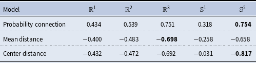
Overall, WAIC favors the three dimensional Euclidean model $\mathbb{R}^3$
, with
$\mathbb{R}^3$
, with $\mathbb{R}^2$
also performing well, while
$\mathbb{R}^2$
also performing well, while $\mathbb{S}^2$
attains intermediate values that are close to those of the best Euclidean specifications. This indicates that increasing the Euclidean dimension improves in sample fit, but that the spherical model in
$\mathbb{S}^2$
attains intermediate values that are close to those of the best Euclidean specifications. This indicates that increasing the Euclidean dimension improves in sample fit, but that the spherical model in $\mathbb S^2$
achieves a comparable average log likelihood under a more constrained geometry. In contrast, the one dimensional spherical model
$\mathbb S^2$
achieves a comparable average log likelihood under a more constrained geometry. In contrast, the one dimensional spherical model $\mathbb{S}^1$
shows poorer WAIC, reflecting the limited flexibility of a circle for this network. Taken together, these results suggest that the spherical models are competitive in terms of overall fit, with
$\mathbb{S}^1$
shows poorer WAIC, reflecting the limited flexibility of a circle for this network. Taken together, these results suggest that the spherical models are competitive in terms of overall fit, with $\mathbb{S}^2$
in particular striking a balance between parsimony, geometric interpretability, and likelihood based performance. These conclusions are based on benchmark social science networks and should be interpreted as illustrative of the potential advantages of bounded latent geometries rather than as universal dominance over Euclidean formulations.
$\mathbb{S}^2$
in particular striking a balance between parsimony, geometric interpretability, and likelihood based performance. These conclusions are based on benchmark social science networks and should be interpreted as illustrative of the potential advantages of bounded latent geometries rather than as universal dominance over Euclidean formulations.
Once central nodes are identified, we detect communities by clustering each latent space. Point estimates of latent positions are obtained and used in spectral clustering (Ng et al., Reference Ng, Jordan and Weiss2002) with geometry-consistent affinity matrices. The number of clusters is chosen via the silhouette score, and the partition with maximum modularity is taken as the representative structure. Figure 6 shows the detected communities, their counts, and modularity scores. The $\mathbb{S}^1$
model achieves the highest modularity, indicating the best capture of the network’s community structure. This is consistent with the directional organization induced by the spherical geometry on
$\mathbb{S}^1$
model achieves the highest modularity, indicating the best capture of the network’s community structure. This is consistent with the directional organization induced by the spherical geometry on $\mathbb S^1$
, which tends to place densely connected families in compact angular sectors while maintaining separation between factions.
$\mathbb S^1$
, which tends to place densely connected families in compact angular sectors while maintaining separation between factions.
Taking together the results in Table 3 and the modularity scores in Figure 6, we see that the model in $\mathbb S^2$
essentially matches the model in
$\mathbb S^2$
essentially matches the model in $\mathbb R^3$
in terms of the correlation between degree and connection based centrality, and it provides the strongest alignment between radial position and degree through the center distance metric. By contrast, the model in
$\mathbb R^3$
in terms of the correlation between degree and connection based centrality, and it provides the strongest alignment between radial position and degree through the center distance metric. By contrast, the model in $\mathbb S^1$
exhibits weaker correlations with degree, which is consistent with its more rigid one dimensional structure. Combining these results with the modularity scores, we see that
$\mathbb S^1$
exhibits weaker correlations with degree, which is consistent with its more rigid one dimensional structure. Combining these results with the modularity scores, we see that $\mathbb S^1$
offers a very sharp community partition along the circle, while
$\mathbb S^1$
offers a very sharp community partition along the circle, while $\mathbb S^2$
yields slightly lower but still competitive modularity together with a latent geometry that supports both clustering and prediction.
$\mathbb S^2$
yields slightly lower but still competitive modularity together with a latent geometry that supports both clustering and prediction.
Clustering across latent space representations, showing number of communities $K$
and modularity
$K$
and modularity $M$
.
$M$
.
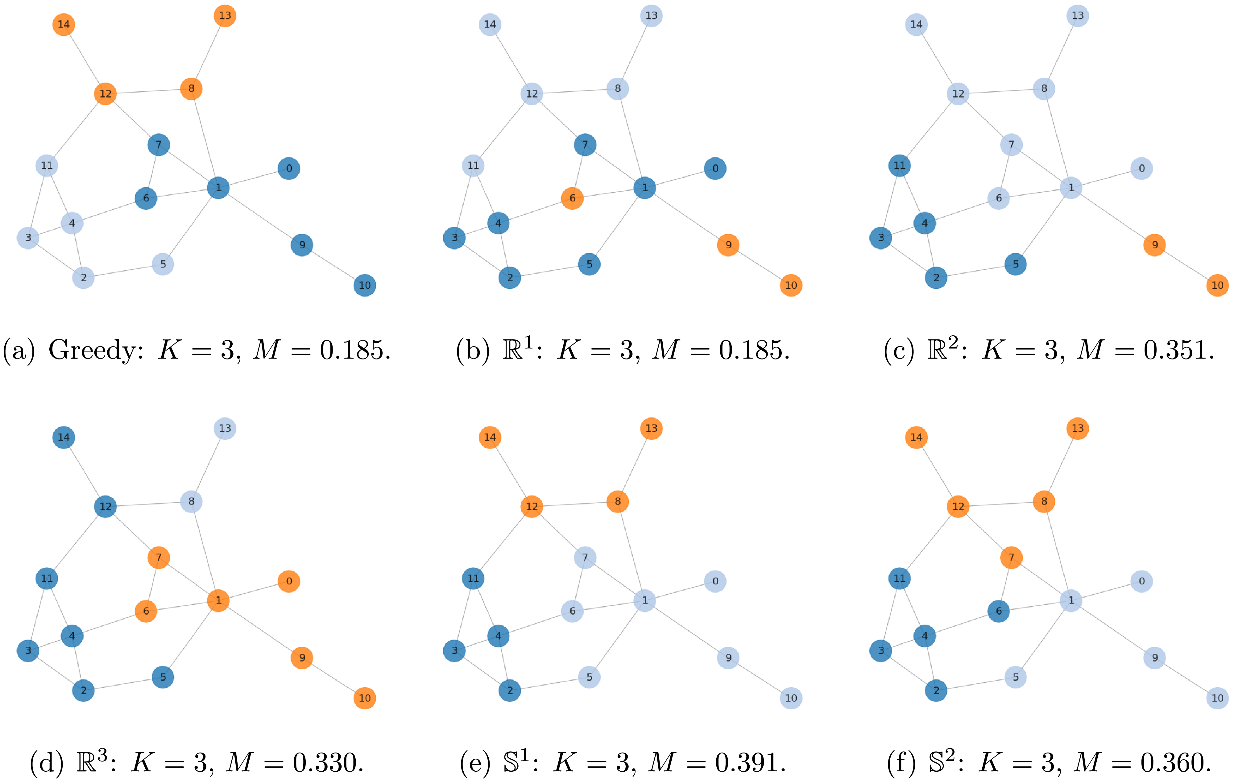
Model adequacy was evaluated through posterior predictive checks using key network-level statistics: degree distribution, geodesic distances, shared edges, and triad census (Figure 7). In this network, latent space models primarily capture degree and geodesic distance patterns, as evidenced by the posterior predictive $p$
-values and the inclusion of observed statistics within the posterior predictive intervals (Gelman et al., Reference Gelman, Hwang and Vehtari2014). For statistics requiring connectedness, computations use the largest connected component of simulated networks drawn from the posterior. Modularity is computed for both observed and simulated networks using the Clauset–Newman–Moore greedy maximization algorithm (Clauset et al., Reference Clauset, Newman and Moore2004).
$p$
-values and the inclusion of observed statistics within the posterior predictive intervals (Gelman et al., Reference Gelman, Hwang and Vehtari2014). For statistics requiring connectedness, computations use the largest connected component of simulated networks drawn from the posterior. Modularity is computed for both observed and simulated networks using the Clauset–Newman–Moore greedy maximization algorithm (Clauset et al., Reference Clauset, Newman and Moore2004).
Posterior predictive checks for all models using network-level statistics in the Florentine families example. Each plot shows model-based histograms with means (dashed line) and the observed value (black line), with the legend reporting the posterior predictive $p$
-value for each model.
$p$
-value for each model.
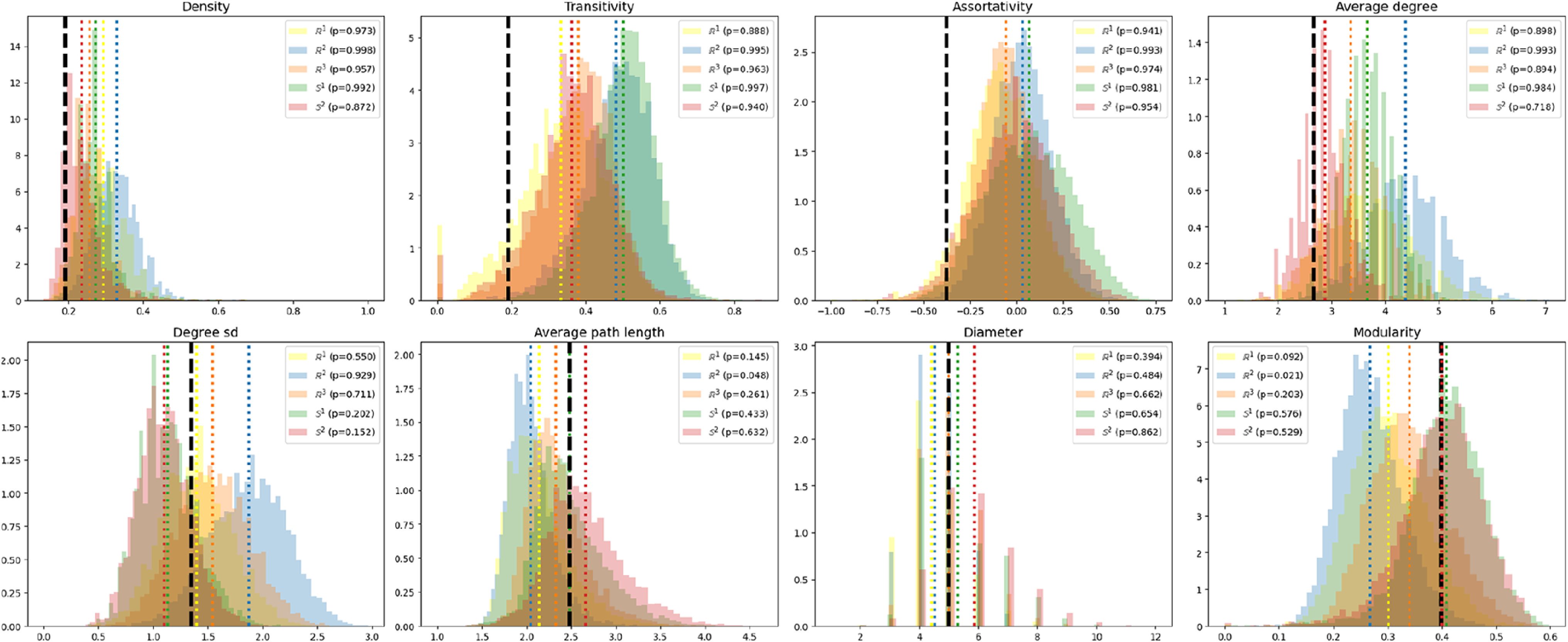
Receiver operating characteristic (ROC) curves for each model.
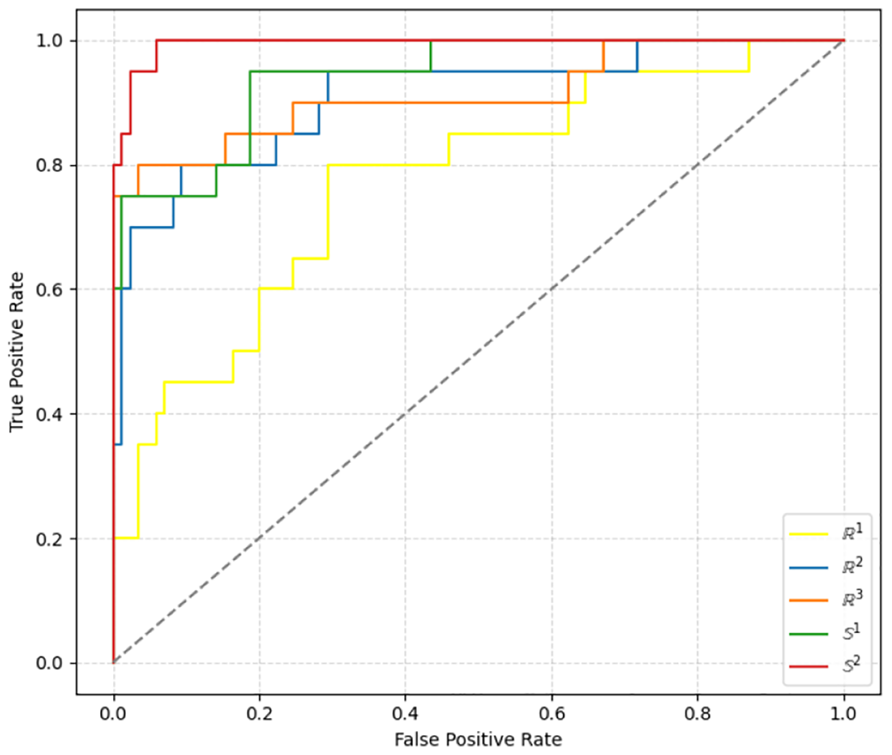
Finally, predictive performance was assessed using out of sample AUC, accuracy and F1 score (Figure 8 and Table 4). The model in $\mathbb S^2$
attains the highest values across all three metrics, with clear gains over the Euclidean models in
$\mathbb S^2$
attains the highest values across all three metrics, with clear gains over the Euclidean models in $\mathbb R^2$
and
$\mathbb R^2$
and $\mathbb R^3$
, and even the simpler model in
$\mathbb R^3$
, and even the simpler model in $\mathbb S^1$
improves on the lower dimensional Euclidean specifications. Higher AUC and F1 score indicate better discrimination between ties and non ties and a more balanced recovery of present and absent edges. These patterns show that spherical latent spaces, particularly
$\mathbb S^1$
improves on the lower dimensional Euclidean specifications. Higher AUC and F1 score indicate better discrimination between ties and non ties and a more balanced recovery of present and absent edges. These patterns show that spherical latent spaces, particularly $\mathbb S^2$
, can exploit curvature and angular separation, together with bounded inner products that stabilize tie probabilities, to represent transitivity, clustering and overlapping directional communities more faithfully than Euclidean alternatives, and that these geometric advantages translate into tangible gains in predictive performance.
$\mathbb S^2$
, can exploit curvature and angular separation, together with bounded inner products that stabilize tie probabilities, to represent transitivity, clustering and overlapping directional communities more faithfully than Euclidean alternatives, and that these geometric advantages translate into tangible gains in predictive performance.
Predictive performance metrics for each model
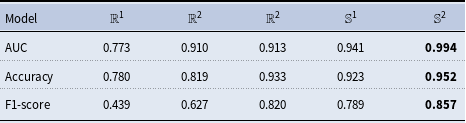
5. Discussion
This paper introduces a spherical latent space model for social network analysis, extending Hoff et al. (Reference Hoff, Raftery and Handcock2002) by embedding nodes on a hypersphere instead of in Euclidean space. This geometry naturally captures transitivity, directional clustering, and cyclic structures while avoiding degeneracies such as unbounded distances. The approach reflects a broader trend in statistics and machine learning toward manifold-based modeling, that provide intrinsic structures for representing hierarchies, cycles, symmetries, and other topological constraints difficult to model in Euclidean settings. Within this framework, latent space models on manifolds offer principled representations of network geometry, enabling faithful structural characterization and interpretable visualizations. Our empirical results show that these geometric properties translate into higher modularity for $\mathbb S^1$
and improved AUC, accuracy, and F1 scores for
$\mathbb S^1$
and improved AUC, accuracy, and F1 scores for $\mathbb S^2$
when compared with Euclidean counterparts, indicating that spherical latent spaces can provide competitive predictive performance and community detection results relative to Euclidean specifications in this empirical setting. These methodological developments and empirical findings constitute the central contributions of this work, namely the formulation and Bayesian implementation of spherical latent space models and their detailed comparison with Euclidean specifications on the Florentine marriage network.
$\mathbb S^2$
when compared with Euclidean counterparts, indicating that spherical latent spaces can provide competitive predictive performance and community detection results relative to Euclidean specifications in this empirical setting. These methodological developments and empirical findings constitute the central contributions of this work, namely the formulation and Bayesian implementation of spherical latent space models and their detailed comparison with Euclidean specifications on the Florentine marriage network.
Several recent contributions have incorporated circular or spherical geometry in network related models, including one dimensional circular visualizations in Hoff et al. (Reference Hoff, Raftery and Handcock2002), spherical latent structure for aggregated relational data in McCormick and Zheng (Reference McCormick and Zheng2015), generative models on the sphere in Smith et al. (Reference Smith, Asta and Calder2019) and Papamichalis et al. (Reference Papamichalis, Turnbull, Lunagomez and Airoldi2022), and methods for detecting the curvature of the underlying latent geometry in Lubold et al. (Reference Lubold, Chandrasekhar and McCormick2023). Our approach is complementary. We assume spherical geometry from the outset and study its implications in a latent distance model for individual level social network data, with an emphasis on Bayesian inference via Hamiltonian based MCMC and on an empirical comparison with Euclidean latent spaces in the Florentine marriage network.
Spherical latent spaces naturally encode relationships with topological constraints such as cyclicity or periodicity, relevant to settings from social networks to recurring spatial processes. By mapping unobserved relationships to positions on the manifold, they support probabilistic inference and interpretable visualizations of complex structures. However, manifold embeddings constrain the parameter space, may impose unnecessary geometric restrictions, and increase computational cost, especially in Bayesian settings with Hamiltonian or geodesic dynamics. In these contexts, directional statistics are essential, redefining concepts like mean, variance, and independence in terms of geodesic distances and angular metrics. Tools such as the von Mises–Fisher distribution, geodesic means, and angular concentration measures enable coherent inference in these nonlinear domains. Empirical results suggest that spherical models can achieve competitive performance relative to Euclidean alternatives in prediction and community detection for the networks studied here.
Future work includes adopting variational inference as a scalable alternative to Monte Carlo methods, lowering computational cost while preserving the model’s geometric structure. Another direction is refining MCMC estimation through better tuning of step sizes, proposals, and acceptance criteria, along with adaptive algorithms and parallel chain diagnostics, enhancements that could improve convergence, posterior exploration, and parameter reliability, particularly in low-dimensional or geometrically constrained settings. Methodological extensions include exploring latent structures beyond the symmetric inner product, such as bilinear forms, asymmetric kernels, or other geometric operators, enabling richer relational patterns and the modeling of directed networks by relaxing the symmetry assumption. The framework can also be extended to multilayer and dynamic networks by modeling latent trajectories that evolve over time or span multiple interaction layers, with the geometry adapting to reflect structural changes and contextual information.
From a broader perspective, extending the geometric stock to hyperbolic spaces or other embedded manifolds would allow model geometry to be tailored to specific domains. Such developments would enable systematic study of how geometric assumptions affect fit, predictive accuracy, and interpretability, advancing manifold-based latent space modeling for complex networks.
Acknowledgments
None.
Supplementary material
The supplementary material for this article can be found at https://doi.org/10.1017/nws.2026.10032.
Data availability statement
All data are publicly available online.
Funding statement
This research received no specific grant from any funding agency, commercial, or not-for-profit sectors.
Competing interests
The authors declare that they have no known competing financial interests or personal relationships that could have appeared to influence the work reported in this article.
Statements and declarations
During the preparation of this work, the authors used ChatGPT-5.2 in order to improve language and readability. After using this tool, the authors reviewed and edited the content as needed and take full responsibility for the content of the publication.
Appendix A. Illustration: Rosenbrock function
In order to illustrate the sampling algorithms given above, we consider sampling from a target distribution of the form $f(\mathbf{x}) \propto {\exp}(-R(\mathbf{x}))$
, where
$f(\mathbf{x}) \propto {\exp}(-R(\mathbf{x}))$
, where $R(\mathbf{x})$
is the Rosenbrock function (Rosenbrock, Reference Rosenbrock1960) given by:
$R(\mathbf{x})$
is the Rosenbrock function (Rosenbrock, Reference Rosenbrock1960) given by:
 \begin{equation*} R(x_1,x_2) = (a-x_{1})^{2} + b \big(x_{2}-x_{1}^{2}\big)^{2}, \qquad \mathbf{x} \in \mathbb{R}^2 \,\, \text{or} \,\, \mathbb{S}^{1}, \end{equation*}
with parameters $a \in \mathbb{R}$
and
$a \in \mathbb{R}$
and $b \in \mathbb{R}$
, with
$b \in \mathbb{R}$
, with $b\gt 0$
. The purpose of this example is not to replicate the latent space model itself, but to provide a controlled benchmark that isolates the geometric challenges faced by the sampling algorithms. In latent space models, and particularly in the spherical formulation considered in this paper, the posterior distribution of latent positions can exhibit strong curvature, anisotropy, and narrow high-density regions due to dependence induced by the network likelihood and geometric constraints. The Rosenbrock function is a standard test case with these characteristics, featuring a curved, narrow valley that is difficult to explore with random-walk proposals. As such, it provides a useful proxy for understanding how Metropolis–Hastings, Hamiltonian Monte Carlo, and GHMC behave in posterior landscapes with similar geometric features to those arising in latent space models.
$b\gt 0$
. The purpose of this example is not to replicate the latent space model itself, but to provide a controlled benchmark that isolates the geometric challenges faced by the sampling algorithms. In latent space models, and particularly in the spherical formulation considered in this paper, the posterior distribution of latent positions can exhibit strong curvature, anisotropy, and narrow high-density regions due to dependence induced by the network likelihood and geometric constraints. The Rosenbrock function is a standard test case with these characteristics, featuring a curved, narrow valley that is difficult to explore with random-walk proposals. As such, it provides a useful proxy for understanding how Metropolis–Hastings, Hamiltonian Monte Carlo, and GHMC behave in posterior landscapes with similar geometric features to those arising in latent space models.
Thus, we apply the Metropolis–Hastings algorithm (Algorithm 2), Hamiltonian Monte Carlo (Algorithm 3), and Geodesic Hamiltonian Monte Carlo (Algorithm 4). In the experiments, the Rosenbrock parameters are set to $a = 1.0$
and
$a = 1.0$
and $b = 5.0$
. For the Euclidean case
$b = 5.0$
. For the Euclidean case $\mathbb{R}^2$
, we use initial state
$\mathbb{R}^2$
, we use initial state $\mathbf{x}^{(0)}=(0.0,0.0)$
,
$\mathbf{x}^{(0)}=(0.0,0.0)$
, $5000$
samples, step size
$5000$
samples, step size $0.05$
, burn-in
$0.05$
, burn-in $50000$
, thinning
$50000$
, thinning $100$
, and
$100$
, and $2$
chains. For the circular manifold
$2$
chains. For the circular manifold $\mathbb{S}^1$
, we use initial state
$\mathbb{S}^1$
, we use initial state $\mathbf{x}^{(0)}=(1.0,0.0)$
with the same sampling settings. These configurations ensured adequate exploration of the target distributions while keeping computational cost reasonable (full implementation details are available at https://github.com/cnosa/Latentspacemodels_Networks).
$\mathbf{x}^{(0)}=(1.0,0.0)$
with the same sampling settings. These configurations ensured adequate exploration of the target distributions while keeping computational cost reasonable (full implementation details are available at https://github.com/cnosa/Latentspacemodels_Networks).
The sampling results for the Rosenbrock distribution are presented in Figure 9 and Table 5. Panels (a) and (b) show the contours of the Rosenbrock function and the sample distributions in $\mathbb{R}^2$
obtained with the MH and HMC algorithms, respectively. HMC more effectively explores the narrow curved valley of the Rosenbrock function, yielding samples with lower variance than MH, which exhibits broader dispersion. Panels (c) and (d) display the Rosenbrock function evaluated on the circle and the corresponding samples under the constraint
$\mathbb{R}^2$
obtained with the MH and HMC algorithms, respectively. HMC more effectively explores the narrow curved valley of the Rosenbrock function, yielding samples with lower variance than MH, which exhibits broader dispersion. Panels (c) and (d) display the Rosenbrock function evaluated on the circle and the corresponding samples under the constraint $\mathbb{S}^1$
. Here, MH produces a more limited exploration than Geodesic HMC, reflected in lower sample variance; in both cases, the estimates reveal a bimodal distribution along the circumference.
$\mathbb{S}^1$
. Here, MH produces a more limited exploration than Geodesic HMC, reflected in lower sample variance; in both cases, the estimates reveal a bimodal distribution along the circumference.
Comparison of Metropolis–Hastings (MH) and Hamiltonian Monte Carlo (HMC) algorithms for sampling from the Rosenbrock distribution on $\mathbb{R}^2$
and
$\mathbb{R}^2$
and $\mathbb{S}^1$
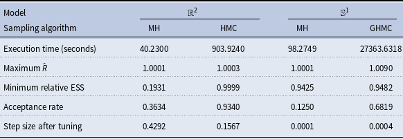
Comparison of sampling results for the rosenbrock distribution across different spaces and algorithms.
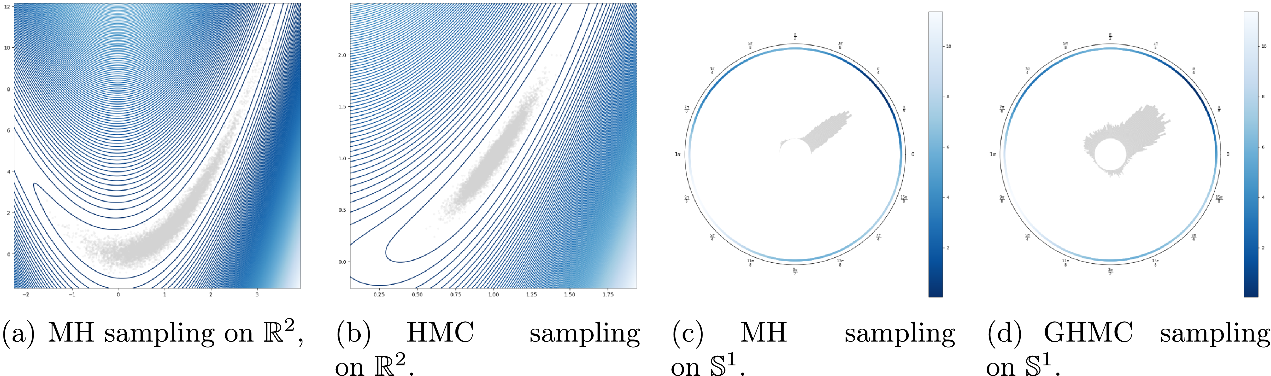
Table 5 reports quantitative performance metrics, including average execution time, maximum $\hat {R}$
, minimum relative ESS, average acceptance rate, mean value of the Rosenbrock function, and the tuned step size. HMC consistently achieves higher acceptance rates and larger ESS, indicating better convergence and more efficient exploration of the target distribution. In contrast, MH shows lower acceptance rates and reduced ESS, reflecting slower mixing, but with substantially lower computational cost, as evidenced by shorter execution times.
$\hat {R}$
, minimum relative ESS, average acceptance rate, mean value of the Rosenbrock function, and the tuned step size. HMC consistently achieves higher acceptance rates and larger ESS, indicating better convergence and more efficient exploration of the target distribution. In contrast, MH shows lower acceptance rates and reduced ESS, reflecting slower mixing, but with substantially lower computational cost, as evidenced by shorter execution times.
Differences between the $\mathbb R^2$
and
$\mathbb R^2$
and $\mathbb S^1$
columns arise because these correspond to distinct target distributions, one defined on the full Euclidean plane and one restricted to the circle. Within each space, discrepancies across algorithms reflect differences in how effectively they explore the high density region. For example, in
$\mathbb S^1$
columns arise because these correspond to distinct target distributions, one defined on the full Euclidean plane and one restricted to the circle. Within each space, discrepancies across algorithms reflect differences in how effectively they explore the high density region. For example, in $\mathbb R^2$
the HMC sampler is able to traverse the narrow curved valley of the Rosenbrock function and spends more time near its minimum, producing a substantially lower average value of
$\mathbb R^2$
the HMC sampler is able to traverse the narrow curved valley of the Rosenbrock function and spends more time near its minimum, producing a substantially lower average value of $R(\cdot ,\cdot )$
than random walk Metropolis, which mixes poorly and remains in higher valued regions. This example is included as a controlled benchmark to illustrate the relative efficiency and robustness of MH, HMC, and GHMC in exploring curved and anisotropic target distributions. These geometric features are representative of posterior distributions arising in latent space models, particularly under spherical constraints.
$R(\cdot ,\cdot )$
than random walk Metropolis, which mixes poorly and remains in higher valued regions. This example is included as a controlled benchmark to illustrate the relative efficiency and robustness of MH, HMC, and GHMC in exploring curved and anisotropic target distributions. These geometric features are representative of posterior distributions arising in latent space models, particularly under spherical constraints.
Appendix B. Model extensions
Under the Bayesian paradigm, the spherical latent space formulation admits several natural extensions that enhance modeling flexibility, allow richer structural assumptions, and facilitate scalability in more complex settings. Below, we outline representative extensions together with their mathematical specifications.
Mixed effects model. Let $\mathbf{x}_{i,j} \in \mathbb{R}^p$
denote covariates associated with the actor pair
$\mathbf{x}_{i,j} \in \mathbb{R}^p$
denote covariates associated with the actor pair $(i,j)$
. The linear predictor can be extended to
$(i,j)$
. The linear predictor can be extended to $\eta _{i,j} = \alpha + \boldsymbol{\gamma }^{\top} \mathbf{x}_{i,j} + \beta \langle \mathbf{z}_i, \mathbf{z}_j \rangle$
, where
$\eta _{i,j} = \alpha + \boldsymbol{\gamma }^{\top} \mathbf{x}_{i,j} + \beta \langle \mathbf{z}_i, \mathbf{z}_j \rangle$
, where $\boldsymbol{\gamma } \in \mathbb{R}^p$
are regression coefficients. Priors for
$\boldsymbol{\gamma } \in \mathbb{R}^p$
are regression coefficients. Priors for $\boldsymbol{\gamma }$
include Gaussian for regularization, Laplace for shrinkage, or horseshoe for sparse, high-dimensional settings. This specification enables joint inference on covariate effects and latent geometry.
$\boldsymbol{\gamma }$
include Gaussian for regularization, Laplace for shrinkage, or horseshoe for sparse, high-dimensional settings. This specification enables joint inference on covariate effects and latent geometry.
Weighted inner product model. Analogous to the eigenmodel, the linear predictor can be generalized to $\eta_{i,j} = \alpha + \beta \,\mathbf{z}_{i}^{\top} {\Lambda } \mathbf{z}_j$
, with
$\eta_{i,j} = \alpha + \beta \,\mathbf{z}_{i}^{\top} {\Lambda } \mathbf{z}_j$
, with $\boldsymbol{\Lambda } = \textsf {diag}(\lambda _1,\ldots ,\lambda _{d-1})$
, assigns dimension-specific weights. This allows certain hypersphere dimensions to influence tie probabilities more strongly, with Normal or hierarchical shrinkage priors on the diagonal elements of
$\boldsymbol{\Lambda } = \textsf {diag}(\lambda _1,\ldots ,\lambda _{d-1})$
, assigns dimension-specific weights. This allows certain hypersphere dimensions to influence tie probabilities more strongly, with Normal or hierarchical shrinkage priors on the diagonal elements of $\boldsymbol{\Lambda }$
controlling effective rank and mitigating overparameterization.
$\boldsymbol{\Lambda }$
controlling effective rank and mitigating overparameterization.
Finite mixture prior. To capture latent community structure, we assign a finite mixture prior to the latent positions $\mathbf{z}_i \mid \xi _i, \boldsymbol{\mu }_{\xi _i}, \kappa _{\xi _i} \overset {\text{ind}}{\sim } \textsf {vMF}(\boldsymbol{\mu }_{\xi _i}, \kappa _{\xi _i})$
, with
$\mathbf{z}_i \mid \xi _i, \boldsymbol{\mu }_{\xi _i}, \kappa _{\xi _i} \overset {\text{ind}}{\sim } \textsf {vMF}(\boldsymbol{\mu }_{\xi _i}, \kappa _{\xi _i})$
, with $\xi _i \overset {\text{iid}}{\sim } \textsf {Cat}(\boldsymbol{\pi })$
, and
$\xi _i \overset {\text{iid}}{\sim } \textsf {Cat}(\boldsymbol{\pi })$
, and $\boldsymbol{\pi } \sim \textsf {Dir}(\boldsymbol{\alpha })$
controlling the cluster weights. This specification induces clustering in the spherical latent space, producing interpretable block structures while preserving the manifold’s geometric constraints.
$\boldsymbol{\pi } \sim \textsf {Dir}(\boldsymbol{\alpha })$
controlling the cluster weights. This specification induces clustering in the spherical latent space, producing interpretable block structures while preserving the manifold’s geometric constraints.
Dirichlet process prior. A nonparametric alternative replaces the finite mixture with a Dirichlet process (DP) prior, $\mathbf{z}_i \mid G \overset {\text{iid}}{\sim } G$
, with
$\mathbf{z}_i \mid G \overset {\text{iid}}{\sim } G$
, with $G \sim \textsf {DP}(\alpha _0, G_0)$
, where
$G \sim \textsf {DP}(\alpha _0, G_0)$
, where $\alpha _0$
is a concentration parameter and
$\alpha _0$
is a concentration parameter and $G_0$
is a suitable base measure on
$G_0$
is a suitable base measure on $\mathbb{S}^{d-1}$
, such as a
$\mathbb{S}^{d-1}$
, such as a $\textsf {vMF}(\boldsymbol{\mu }_0, \kappa _0)$
distribution. The DP formulation enables the number of latent clusters to be inferred directly from the data, preserving the geometric constraints of the spherical latent space.
$\textsf {vMF}(\boldsymbol{\mu }_0, \kappa _0)$
distribution. The DP formulation enables the number of latent clusters to be inferred directly from the data, preserving the geometric constraints of the spherical latent space.
Multilayer networks. For multiplex or multilayer relational data $\mathbf{Y}_1,\ldots ,\mathbf{Y}_L$
, the linear predictor in layer
$\mathbf{Y}_1,\ldots ,\mathbf{Y}_L$
, the linear predictor in layer $\ell$
can be expresed as
$\ell$
can be expresed as $\eta _{i,j,\ell } = \alpha _\ell + \beta _\ell \langle \mathbf{z}_i, \mathbf{z}_j \rangle$
, with layer-specific intercepts
$\eta _{i,j,\ell } = \alpha _\ell + \beta _\ell \langle \mathbf{z}_i, \mathbf{z}_j \rangle$
, with layer-specific intercepts $\alpha _\ell$
and similarity coefficients
$\alpha _\ell$
and similarity coefficients $\beta _\ell$
assigned hierarchical Normal priors to enable information sharing across layers, thus capturing both layer-specific tie formation mechanisms and cross-layer dependencies.
$\beta _\ell$
assigned hierarchical Normal priors to enable information sharing across layers, thus capturing both layer-specific tie formation mechanisms and cross-layer dependencies.
Dynamic networks. For temporal networks $\mathbf{Y}_1,\ldots ,\mathbf{Y}_T$
, latent positions
$\mathbf{Y}_1,\ldots ,\mathbf{Y}_T$
, latent positions $\mathbf{z}_{i,t}$
can be assigned a first-order Markov process on the sphere via
$\mathbf{z}_{i,t}$
can be assigned a first-order Markov process on the sphere via $\mathbf{z}_{i,t} \mid \mathbf{z}_{i,t-1} \sim \textsf {vMF}(\mathbf{z}_{i,t-1},\kappa _z)$
, while layer-specific intercepts and similarity coefficients evolve as
$\mathbf{z}_{i,t} \mid \mathbf{z}_{i,t-1} \sim \textsf {vMF}(\mathbf{z}_{i,t-1},\kappa _z)$
, while layer-specific intercepts and similarity coefficients evolve as $\alpha _t \mid \alpha _{t-1} \sim \textsf {N}(\alpha _{t-1},\sigma _{\alpha }^2)$
and
$\alpha _t \mid \alpha _{t-1} \sim \textsf {N}(\alpha _{t-1},\sigma _{\alpha }^2)$
and $\beta _t \mid \beta _{t-1} \sim \textsf {N}(\beta _{t-1},\sigma _{\beta }^2)$
, introducing Markovian dependence that allows the model to capture smooth temporal variation in both latent geometry and tie formation tendencies.
$\beta _t \mid \beta _{t-1} \sim \textsf {N}(\beta _{t-1},\sigma _{\beta }^2)$
, introducing Markovian dependence that allows the model to capture smooth temporal variation in both latent geometry and tie formation tendencies.
Alternative computational strategies. While MCMC is the standard inference approach for latent space models, alternative methods can improve scalability. Variational inference (e.g., Blei et al., Reference Blei, Kucukelbir and McAuliffe2017) and stochastic variational inference (e.g., Hoffman et al., Reference Hoffman, Blei, Wang and Paisley2013) provide deterministic approximations to the posterior, with stochastic gradient optimization enabling application to large-scale networks.
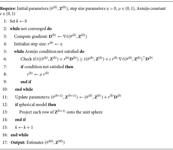
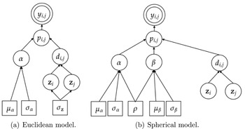
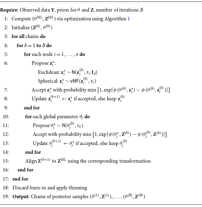
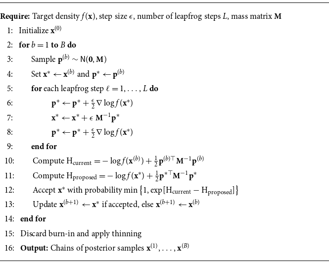
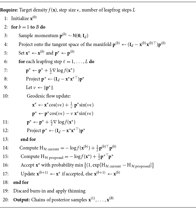
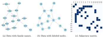
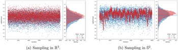


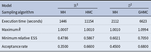


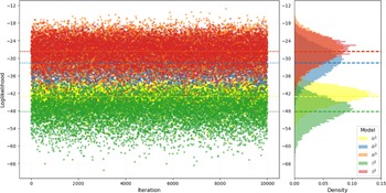
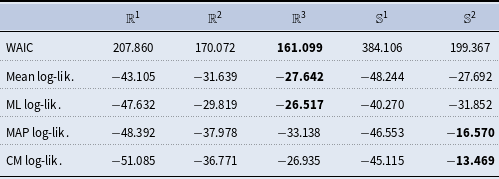
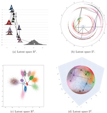


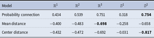
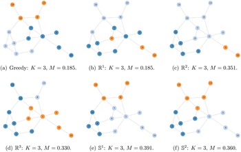


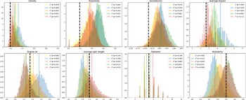


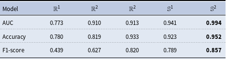
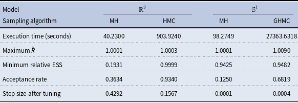


 Open access

