


Introduction
On the basis of a recent experimental study done on the confluence area of Unteraargletscher, Bernese Alps, Switzerland, it has been suggested (Reference Gudmundsson,, Iken, and Funk,Gudmundsson and others, 1997) that the distinctive character of the strain-rate regime of a glacier confluence is related to: (1) an increase in ice thickness in the flow direction from the junction point towards the center of the confluence; (2) an overall change in the mean flow direction of the two tributaries as they enter the confluence area; and (3) a general increase in surface velocity along the center line from the junction point towards the confluence center. To gain a somewhat better understanding of the flow characteristics, and to test these ideas against numerical and analytical models, two rather simple two-dimensional (2-D) conceptual models are introduced that focus on the first and the third mechanisms listed above. The first model is a numerical flowline model involving balances over a longitudinal vertical section running from the junction point towards the center of the confluence. This model is used to understand the effect of increased ice thickness in the flow direction on the ice-deformational pattern with depth. In particular, the vertical strain-rate variation with depth for different sets of basal boundary conditions is investigated. The second model is a map-plane model of the surface area of the confluence. It is used to elucidate the horizontal strain-rate pattern caused by a no-slip/free-slip transition at the margin.
It is clear that the flow regime of a confluence area must in general be expected to vary strongly in all three spatial dimensions, and one might therefore expect 2-D models to be of limited help in understanding such a complicated three-dimensional (3-D) flow pattern. I will, however, argue that most of the flow characteristics of a glacier confluence can be understood within the framework of simple 2-D models. This is an important observation because, among other things, sensitivity studies can be carried out so much more easily with 2-D models. On the other hand, for an exact comparison of field measurements with calculations of flow based on Glen’s flow law, a fully 3-D model will evidently be needed. This type of comparison can be found in Reference Gudmundsson,Gudmundsson (1994a).
The discussion is limited to confluences for which the two tributaries are more or less similar in size. The point of the glacier margins where the marginal zones of the two tributaries converge is referred to as the junction point. The margins of the confluence containing the junction point are called the “inner” margins of the confluence. The marginal surficial detritus of the inner margins merges at the junction point to form the surface debris of the medial moraine. The two margins of the tributaries, which together form the margins of the coalesced glacier, are referred to as the “outer” margins of the confluence.
This paper is divided into two main parts titled “flow-line model” and “map-plane model”. The discussion of the map-plane model is divided into two further sections, which deal with the analytical and the numerical solutions of this problem. For the first part, and for each of the sections of the second part, the results are given and discussed separately.
Field Equations
For both the flowline and the map-plane models the field equations are


where Vi are the velocity components, ρ the ice density, fi the components of the body force, and σij the components of the Cauchy stress tensor. In the numerical calculations, Glen’s flow law is used:

where ⋵ij are the strain rates. The deviatoric stresses are

and σ′π the second invariant of the deviatoric stress tensor, is defined as
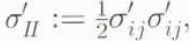
where δij is the Kronecker delta. The analytical models are only valid for a linear medium where n = 1. The notation is summarized in Table 1.
Part I: Flowline Model
Motivations and model definition
Measurements in boreholes drilled at the confluence area of Unteraargletscher of the vertical displacements of magnetic rings over time revealed surprisingly complicated variations in vertical strain rates with depth (Reference Gudmundsson,, Iken, and Funk,Gudmundsson and others, 1997). The vertical strain rates are positive (extension) at the surface, but strongly negative (compression) at the base. This type of vertical strain-rate variation is considerably more complicated than the constant, or linear, vertical strain-rate depth profile often used in the glaciological literature (e.g. Reference Paterson,Paterson, 1994), and it is, hence, of interest to know what factors are responsible for this complicated strain-rate profile.
List of symbols

In the following, I will argue that — at least if basal velocity is of secondary importance to ice creep — this type of vertical strain-rate variation occurs whenever the ice thickness increases in the flow direction. It is the thickness increase together with a particular set of boundary conditions which gives rise to the observed strain-rate variation. This type of vertical strain-rate pattern is therefore not limited to a confluence area, but the longitudinal section along the center line of a confluence is a region where it must be expected to be especially pronounced.
To exemplify the effect of an increase in ice thickness in the flow direction on the vertical strain-rate variation, a sinusoidal-shaped bed-line is employed as a convenient idealization of the bed geometry. The analysis of the flow is facilitated by the fact that analytical solutions, which were derived for n = 1 and the limiting case ak ≪ 1, where k is the wavenumber (Reference Nye,Nye, 1969; Reference Kamb,Kamb, 1970; Reference Morland,Morland, 1976; Reference Gudmundsson,Gudmundsson, 1997a), take a particularly simple form for this type of bed-line geometry.
For numerical calculations of the flow for n ≠ 1 and a finite a the general-purpose FE program MARC was used. A description of the mesh generation, the testing of the FE program, and numerical error estimates are given in Reference Gudmundsson,Gudmundsson (1994a). The flow was calculated for both no-slip and free-slip boundary conditions. These two boundary conditions represent two different limiting situations of no and perfect basal sliding, respectively.
Results from flowline model
For a large number of sinusoidal bed-lines with different amplitude-to-wavelengths ratios, the flow field was calculated for both no-slip and free-slip boundary conditions and for different values of n. For the current purpose it is not necessary to give a systematic overview of all the different resulting flow fields. Only the general pattern of flow is of interest here, and the results will be illustrated by showing calculated vertical velocities and vertical strain rates for one particular model.
Figure 1a shows numerically calculated vertical velocities for a free-slip flow. The values of the model parameters (amplitude a and wavelength λ of the bed profile, mean ice thickness h and surface slope α) are given in the figure caption. The orientation of the coordinate system is such that the x axis is parallel, and the z axis perpendicular, to the mean surface. The bed-line, as a function of x, is denoted by zb(x) and is given by

where a is the amplitude and k the wave number. Only a part of the FE mesh, which has a height and a width of ten times the wavelength λ, is shown.
An analytical solution of the flow valid to second order in ak, and for n = 1 (Reference Morland,Morland 1976, Reference Gudmundsson,Gudmundsson 1997a), shows that maximum vertical velocities are found at the bed at the points of maximum slope, and maximum vertical strain rates are situated at kz = 1 in the limit ak → 0. The vertical strain rates, ⋵zz, are therefore positive throughout the glacier depth where the ice thickness increases in the flow direction, and everywhere negative where the thickness decreases. The numerically calculated vertical velocity field (Fig. 1a) exemplifies this behavior. Figure 1b depicts vertical strain rates for the same model as Figure 1a, and it can be seen that

(a) and (с) Vertical velocities for free-slip and no-slip boundary conditions, respectively. (b) and (d) Vertical strain rates for free-slip and no-slip boundary conditions, respectively. The model parameters are: a = 2 m, λ = 20 m, h =200 m, n = 3, and ρg sin α = 8.99577 × 10≪3 bar m≪1. Velocities are in m a≪1. A part of the FE mesh is shown in (a). The general flow direction is from left to right.

For the no-slip boundary condition the resulting velocity and strain-rate fields (Fig. 1c and d) are quite different than for free-slip boundary conditions (Fig. 1a and b). The vertical velocities now reach their maximum values not at the bed-line, as in Figure 1a, but somewhat above the bed. The reason for this is quite simple. As one proceeds in the z direction from the surface towards the lee side of the peak of the sinusoidal curve, the dip of the velocity vectors changes gradually and approaches the dip of the bed-line. This results in increasingly large vertical velocities with depth. Because of the no-slip boundary condition, vertical velocities (vz ) must, however, be zero along the bed-line, so that vz eventually decreases again as the bed-line is approached. The result is a zone of strong vertical compression in the vicinity of the bed-line below a region of positive vertical strain rates. Where the glacier gets thinner in the flow direction, the situation reverses. Thus, it is the no-slip boundary condition, together with the varying glacier thickness, which forces a reversal in the strain-rate regime from extension/compression towards compression/extension with increasing depth. The exact bed geometry is expected to change only the amplitude of the velocity variations and their extent, but not the main characteristics of the vertical strain-rate variation. (This statement is, however, incorrect for very large values of the amplitude-to-wavelength ratio (Reference Gudmundsson,Gudmundsson, 1997b).) No systematic study was done on how the position of the maximum of vz (Fig. 1c) depends on changes in roughness or material properties. A few calculations with different values of n and ak however, showed that with increasing n and ak the maximum moves towards the bed.
Discussion
The no-slip boundary condition, together with increasing ice thickness along the flow direction, gives rise to a vertical strain-rate pattern that is qualitatively the same as that measured on Unteraargletscher (Reference Gudmundsson,, Iken, and Funk,Gudmundsson and others, 1997). There, vertical strain rates (⋵zz) were positive at the surface, increased somewhat with depth, and then changed from positive values to negative ones close to the bed. Because the actual flow field is expected to vary in all three spatial directions, there will inevitably be some deviations from the plane-strain-rate situation, causing some additional complications that cannot be fully addressed with this simple conceptual 2-D model. For a quantitative comparison a full 3-D model is needed. Still, this simple 2-D model gives a plausible explanation of the measured sign reversal of ⋵zz at a depth of about 220 m. It also clarifies the effect that changes in ice thicknesses have on vertical strain-rate variations, which is helpful in identifying the causes of un-expected flow perturbations seen in more complicated models. The results also Suggest that during the measurement period (second half of September 1991) the bed conditions were closer to no-slip than free-slip in spite of the fact that observations of temporal velocity variations demonstrate that some sliding took place.
Part II Map-Plane Model
Motivation and model definition
Measurements of the deformation of surface ice at the glacier confluence of Kaskawulsh Glacier, Yukon Territory, Canada (Reference Brecher,, Bushnell, and Ragle,Brecher, 1969; Reference Anderton,, Bushnell, and Ragle,Anderton, 1970), and Unteraar-gletscher, Bernese Alps, Switzerland (Reference Gudmundsson,, Iken, and Funk,Gumundsson and others, 1997), have shown the center lines of these glaciers to be subjected to a longitudinal extension and a transverse compression. In the following, I will argue that this deformational pattern can be considered to be a consequence of the abrupt change in boundary conditions at the junction point, and that the effect of this change in boundary conditions on the flow field and the surface topography can be understood within the framework of a relatively simple 2-D map-plane model.
Marginal ice entering a confluence along its inner margins experiences an acceleration as it passes the junction point. There is also a sudden change in boundary conditions at this point. Along the margin, boundary conditions are of the no-slip type. For a symmetrical confluence, nо shear will act on the center line and, if we further assume infinite glacier thickness, one could theoretically put a perfectly lubricated vertical plane along the center line without affecting the velocity or the stress fields. The “boundary” conditions along the center line are thus of the free-slip type. The junction point of the sliced area can be considered to mark the transition from a no-slip to a free-slip boundary condition.
In the model, I assume that the confluence is perfectly symmetrical and infinitely thick. The assumption of infinite thickness restricts the applicability of the results to those sections of a particular confluence where the ice predominantly experiences resistance from the margins rather than from the deeper-lying sections of the bed. The angle between the two identical tributaries is set to zero. There is therefore no prescribed convergence of flowlines. Thickness changes are ignored and plane strain conditions assumed.
Previous work
Flow across a no-slip/free-slip transition has been studied theoretically by Reference Hutter,Hutter and Olunloyo (1980,Reference Hutter, and Olunloyo.1981) and Reference Barcilon, and MacAyeal,Barcilon and MacAyeal (1993). Hutter and Olunloyo found the normal and shear stresses to be singular across the transition point. Barcilon and MacAyeal confirmed and corrected previous results. They found singularities in shear stress and pressure at the point of transition. The singularity in pressure represented an inconsistency with the assumptions made, causing first-order pressure to exceed the zeroth-order pressure. They therefore concluded that the problem remains open and unsolved. Consequently, this problem must (at least for the time being) be solved numerically, which is done below for some specific cases. However, before proceeding to the discussion of the numerical solution, the properties of a closely related problem, which can be solved analytically, will be discussed.
Simplifications which lead to an analytically solvable problem
Part of the difficulty in solving the no-slip/free-slip transition problem lies in the fact that along a section of the margins the velocities are prescribed (i.e. set to zero), but on the remaining section the shear stresses are fixed. If only velocity variations along the interface were to be prescribed, the analytical solution of the corresponding problem would be straightforward.
The velocity variation along a confluence center line will to some extent be determined by factors not incorporated in the 2-D map-plane model, such as surface inclination and bedrock geometry. Hence, even an exact solution of the no-slip/free-slip problem would be only partially applicable to the physical problem considered. From an observational point it is of some value to be able to calculate the velocity field of the confluence for a given velocity variation along the center line, where the general shape of the prescribed velocity variation is based on field measurements. This problem, where the velocity along the center line is an input and not an output, has the great advantage over the no-slip/free-slip transition problem of being, at least for a linear viscous fluid, exactly solvable.
The geometrical shape and the boundary conditions of this simplified model are shown in Figure 2. The analytical solution is given below.
An infinite strip of highly viscous material. The two sets of boundary conditions used in the text are shown. The thick lines represent the glacier boundary, and the dashed line the center line of a conceptual confluence. Only the lower half of the perfectly symmetrical confluence is shown. J denotes the junction point. The origin of the coordinate system is on the lower boundary directly below the junction point.

Analytical Solution of the Simplified Map-Plane Model
Rheological assumptions and field equations
Equations (1)–(3) are non-dimensionalized by scaling the velocities vi, the stresses σij, and the time t with “natural” quantities of the model. For non-dimensional variables upper-case letters are generally used.
Because the width of the channel in the downstream direction of the confluence is 2d, d is the natural length scale. The analytical solutions for the velocity and the shear stress of an infinitely deep channel of uniform width 2d are


where τ := ρgd sin α, and α is the surface slope. The stresses are scaled with τ. A scaling factor for t can be defined as the time it takes for the strain at the wall to reach the value unity. Hence, the following scalings are used:

The non-dimensional velocity Vi is defined by

and the non-dimensional strain rates ⋵ij are given by

The maximum value of Vx is 2(n + 1)τ1. In two dimensions, the non-dimensionalized field equations are then


and Glen’s flow law can be written as

For n = 1 the constitutive equation is Ėij = Σ′ij = Σij + Pδij, Which if substituted into the momentum equation and the equation of continuity leads to


Solution technique for n = 1
For n = 1, Equations (16)–(18) can be solved for an infinite strip with prescribed velocities along the boundaries. Only field perturbations (i.e. anomalous fields) resulting from a prescribed velocity anomaly at the boundaries are considered here, and the part of the flow that is directly gravity-driven is ignored, because it will simply add linearly to the perturbated velocity distribution. Lower-case letters will now be used, and it is to be understood that all variables are dimensionless.
Fourier transformation of the field equations with respect to x leads to


where the Fourier transform is defined as

and i is the imaginary unit. With the help of Equations (19) and (21), p[k,y) can be expressed as a function of vy(k,y), and that expression substituted into Equation (20), resulting in one homogeneous linear differential equation of fourth order for vy(k,y):

This differential equation can easily be solved. The solution is

where the integration functions A(k), B(k), C(k) and D(K) are to be determined through the boundary conditions. The solutions for vy(k, y), p(k, y) and the stresses can also be determined in terms of the integration functions.
The boundary conditions are

and

where τivx c(k) is the Fourier transform of vx(x, 1), which is the applied velocity perturbation along the center line.
Solving the resulting system of equations leads to

where the following abbreviations have been used:


Because of the linearity of the differential equations, the sum of the solutions corresponding tο two different center-line velocity variations can be superimposed to give the solution of the combined velocity variation. To understand the general properties of the solutions, it will therefore suffice to consider the effect of some particularly simple type of velocity perturbation. A harmonic velocity variation is the most logical choice, as it produces anomalous velocity fields of the same form and frequency.
Results derived from analytical solutions
The results can be understood most easily by considering the velocity and the pressure field in (k, y) space. For an illustrative example of the velocity and pressure fields in (x, y) spaee see Reference Gudmundsson,Gudmundsson (1994a).
Longitudinal velocities
Figure 3a shows the square root of the power spectrum of the longitudinal velocity vx(k,y), for 0 ≤ k ≤ 4 π and for vx(k, 1) = 1. Note that the boundary conditions force vx(k, y) to be equal to unity along the y = 1 boundary, and zero for y = 0. The change in relative phase shift of the longitudinal velocity field with respect to a prescribed harmonic velocity variation along the y = 0 boundary is indicated through the sign of the labels and the style of the contour lines in the figure. Positive values and solid lines indicate that for some particular value of x, vx(x,y) points in the same direction as x(x,1), and negative values and dashed lines that the ice is flowing in the opposite direction to the applied center-line velocity perturbation. It can be seen from the figure that the anomalous velocities introduce a flow recirculation which is superimposed on the general flow field. This recirculation is found for all values of k. The dividing line in (k, y) space, which marks the separation from down-glacier flow to up-glacier flow as one proceeds from the center line (y = 1) towards the outer boundary of the confluence (y = 0), is drawn as a thick solid line.
Square-root power spectrum of the anomalous longitudinal velocity vx(k, y) (a), the transversal velocity vy(k, y) (b), and the pressure distribution p(k, y) (с).

The transverse extent of the recirculation zone depends strongly on k. It is largest for k = 0, and the dividing line is in this limit situated at y = 2/3, as can be found by calculating the limit of vx(k, y) as k → 0. For at least two-thirds of the glacier cross-section, the direction of the anomalous velocity flow is then opposite to the direction of the main flow. This will reduce the maximum velocity of the flow up-stream of the junction point and shift it towards the center line. For large-wavelength velocity components this reduction is about 30% of the amplitude of the center-line velocity perturbation, but it decreases with increasing k For k → +∞ the separation line approaches asymptotically y =1.
Transverse velocities
The square root of the power spectrum of the anomalous transverse velocity can be seen in Figure 3b. The transverse velocity is 90° out of phase with the longitudinal velocity. Hence, in the (k,y) space the maximum amplitude of vy(k,y) is obtained along a line which corresponds to the minimum of vx (k, y). This line, which was earlier referred to as the separation line, is drawn in Figure 3b as a thick solid curve. The maximum of the transverse velocities is always obtained within one-third of the glacier width because the separation line is at y ≥ 2/3 for all values of k.
With increasing k the amplitude of vy(k,y) increases, while the transverse extent decreases. Hence, the maximum of vy(k,y) moves towards y = 1, and becomes more localized, causing larger velocity gradients. Because limity→1 ∂vy(k,y)/∂y =k all strain rates go linearly to infinity with k. In the high-frequency limit, all strain rates are infinite and localized at y = 1. This comes as no surprise, as in this limit velocity gradients are effectively forced to become infinite by the boundary conditions. Although these singularities resemble somewhat those resulting from the theoretical treatment of the no-slip/free-slip problem by Reference Hutter,Hutter and Olunloyo (1980, Reference Hutter, and Olunloyo.1981), no comparison can be made, because the two problems are fundamentally different. In the treatment of Hutter and Olunloyo the singularities are predicted, whereas here the singularities are in essence prescribed.
Transverse velocity perturbations can be a substantial fraction of the center-line velocity perturbation, and they will accordingly cause a marked convergence of the flow-lines, resulting in a transverse compression close to the center line and extension close to y = 0. It is important to realize that this convergence takes place although the two arms of the confluence run parallel to each other.
Pressure distribution
The pressure distribution is of interest because lines of constant pressure will correspond, to some extent, to contour lines on the glacier surface. Figure 3c gives the pressure as a function of k and y. There is a pressure drop along the center line for those sections where the applied velocity increases in the flow direction. Where the velocity decreases, the situation reverses. The amplitude of this surface depression is largest where the velocity increases fastest, which generally is close to, or at, the junction point.
The pressure drop depends strongly on k. It can be shown that p(k, 1)/p(k, 0) → ∞ as k → ∞, representing an infinite pressure drop. A similar pressure drop near the transition from no-slip to free-slip has been predicted on theoretical grounds by Reference Barcilon, and MacAyeal,Barcilon and MacAyeal (1993, fig. 6). The long-wavelength limit is: p(k, 1)/p(k, 0) → 1 as k → 0, in which case the pressure drop is almost constant across the width of the glacier. The spatial extent of the surface depression is quite limited for moderate to high k values (Fig. 3c). A sharply defined surface depression of this type can easily be seen on Unteraargletscher as well as on numerous other confluences.
Discussion
Reference Balise, and Raymond.Balise and Raymond (1985) investigated the transfer of basal velocity perturbations to the surface for a linear medium. Their approach bears strong similarities to the solution approach described above.They too found the anomalous velocity to recirculate, but, contrary to what is observed here, only for a certain range of k values. Only short wavelengths, less than about 5.2 times the mean ice thickness, lead to recirculation. This difference is caused by the different boundary conditions at y = 0. Reference Balise, and Raymond.Balise and Raymond (1985) used a free-surface boundary condition allowing the surface to react in such a way as to compensate for the mass transfer caused by the velocity perturbation (although the surface was not allowed to evolve with time). Because of the no-slip boundary conditions at y = 0 applied here, there is no free surface, and internal flow must set up a recirculation to counteract the mass transfer at y = 1 and to ensure mass conservation.
The linear solution of the map-plane problem revealed that a longitudinal extension and a concomitant transverse compression is a direct result of the change in boundary conditions at the junction point. A convergence of the two tributaries is not needed to produce this type of strain-rate regime.
From the shape of the pressure distribution it can be concluded that if the center-line velocity increases with x (which is generally the case for a confluence area), the surface elevation is higher around y = 0 than around y = 1. The amplitude and spatial extent of this surface depression depends primarily on the magnitude of the velocity gradients along the center line. Note that the downward slope from the outer boundaries of the confluence towards the junction point is in fact needed to drive the transverse flow seen in Figure 3b. Superimposed on the general slope of the glacier, this anomalous surface change causes the contour lines to tilt somewhat toward the confluence. Tilting of this type can be seen on Unteraargletscher. Reference Anderton,, Bushnell, and Ragle,Anderton (1970) observed a similar converging of flowlines just below the confluence of the north and the central arm of Kaskawulsh Glacier and, apparently correlated, changes in surface slope.
Numerical Solution of the Map-Plane Model
Geometrical assumptions, boundary conditions
A number of interesting conclusions about the general surface flow pattern of a confluence could be drawn from the analytical solution valid for n = 1. It is therefore of some importance to see to what extent these findings remain qualitatively correct for a non-linear material behavior and for a no-slip/free-slip transition boundary condition, in which case the velocity along the center line is an output of the corresponding model and not simply assumed. This problem must be solved numerically, and for that purpose the FF program MARC was utilized.
The coordinate system used is the same as that of Figure 2. The lower left and upper right corners of the model have the coordinates (−5,0) and (5,1), respectively. Along the lower boundary (y = 0), and along the upper boundary upstream of the junction point, all velocities are set to zего. The junction point is at (x, y) = (0, 1). Along the center line, the ice is allowed to move freely in the x direction. Across the righthand boundary (Fig. 2), all velocities are set equal to the velocities of the corresponding nodes along the lefthand boundary. Hence, the model is periodic, with a period of 10 and width 1. The main advantage of using a periodic boundary condition is that no assumptions about the velocity profile or the stresses along the transverse boundaries need to be made. Note that because the upper right corner of the model is in effect the same point as the upper left corner, there are actually two junction points within the model, lying 5 units apart.
The length of the numerical model must be large enough for a fully developed Poiseuille flow to be established between its two junction points. The development of laminar flow in the entrance of a duct bears some similarity to the idealized confluence. Laminar entry-length solutions can be found in the literature for circular and non-circular ducts and parallel plates. Reference Shah, and London.Shah and London (1978) give the following expression for the entrance length:

valid within ±2% for many duct shapes, where Re is the Reynolds number. The entrance length is defined as the distance from the entrance at which the center-line velocity agrees to within 99% with that of the fully developed Poiseuille flow. For creeping flow, Re ≈ 0 so that xl ≈ 0.6. The distance of 5, from one junction point to the next, can therefore be considered sufficient.
The use of periodic boundary conditions affects the magnitude of the velocities above and below the junction point. For a given driving stress, doubling the channel width leads to an increase of the volumetric flux by a factor of 2n+2. Hence, for a fully developed Poiseuille flow the volumetric flux of the channel in the down-flow direction of the junction point is more than twice the combined flux of the two tributaries of width d. The flux entering the confluence is in this sense too small, and velocities downstream from the junction point are correspondingly smaller, and up-stream larger, than for a fully developed flow. A real glacier would react to this imbalance in fluxes by lowering the driving stress below the junction point until a balance of fluxes in and out of the confluence area is reached. In this conceptual model, no corresponding changes in surface geometry, which is fixed, can develop. As a consequence, the velocity is determined in part by the ratio of the lengths of the two sections above and below the junction point, which for the model calculated was set equal to 1. This will, in turn, influence the magnitude of the velocity gradients over the confluence area. In what follows it will be assumed that the area over which the glacier reacts to velocity gradients does not depend on their magnitude, although the conclusions do not depend critically on this assumption. This assumption is a reasonable one for creeping flow—the entrance length for creeping laminar flow in a duct does, for example, not depend on the inflow velocity — but is not correct if acceleration terms are important (which is not the case).
Three models, with equidistant rectangular meshes but different grid size were used, one with grid size 0.1, i.e. 10 elements over the width of the model and having a total number of 1000 elements, another with grid size 0.05, and a third with grid size 0.025 having a total of 16 000 elements. To test the correctness of the calculations, a channel flow was modeled with velocities at the upper and lower boundaries set to zero. For n = 1 and n = 3, maximum scaled velocities were 1/3.99 and 1/32.16, respectively, whereas the corresponding analytical values are 1/4 and 1/32, respectively. Both calculated numbers refer to the FE mesh with a grid size of 0.05. Results obtained with the 0.05 and 0.025 grid-size meshes differed by less than 0.2%. For the final calculations discussed below, the 0.025 mesh was used.
Solution procedure
The element used was a linear four-node quadrilateral plane-strain element, and the incompressibility of the flow-was enforced with the constant dilatation method. This element does not lock in the incompressibility limit. It cannot represent a singular behavior, and any singularity of the underlying problem is smeared out in the numerical solution over a region comparable in size to the spatial dimensions of the elements. Successive mesh refinement can therefore be used to detect a singularity. As discussed below, the numerical results indeed suggest that longitudinal and transverse strain rates become singular at the junction point, because a strong variation in calculated quantities, such as strain rates and velocities, was detected that became more localized and larger with each successive level of mesh refinement. On the basis of the above discussion, this singularity can be understood to be caused by the high-frequency components introduced by the infinitely high velocity gradients at the junction point
Results from numerical calculations of the no-slip/free-slip problem
The longitudinal velocity (vx ) along the center line for n = 1 and n = 3, as a function of the distance in the downstream direction from the junction point, can be seen in Figure 4a. The velocities were normalized by the maximum of the velocity along the center line.
The longitudinal gradient of the velocity at the junction point (denoted by a J in the figure) is very large. Two observations suggest that the actual asymptotic slope of the curve at the junction point is not accurately represented in the figure, and should be infinite: (1) the slope increased with each successive mesh refinement, and (2) the slope of the calculated curve in Figure 4a changed abruptly at the second nodal point from the junction, the extrapolation of the curve through the other nodal points towards the junction suggesting an even larger slope than that shown in Figure 4a. Except in the immediate vicinity of the junction point, calculated values obtained with the 0.05 and 0.025 grid-size meshes differed by less than 1.2%. An infinite slope means that the longitudinal strain rates (⋵xx), and because of the incompressibility condition also the transverse strain rates (⋵yy), become singular at the junction point.
The velocity gradients increase with n, as can be seen in Figure 4a. For n = 1 and n = 3, 90% of the maximum center-line velocity is reached at x = 0.78 and x = 0.30. respectively. This is a posteriori justification of using a distance of 5 between the two no-slip/free-slip transitions within the model.
Figure 4b depicts the longitudinal and transverse velocities along a transverse profile that traverses the channel at the height of the junction point. Velocities were normalized by the maxima of the longitudinal center-line velocities. The location of the junction point on the x axis is indicated in the figure by J. The maxima of the velocities are shifted somewhat towards the junction point with respect to the geometric center of the channel. This shift is larger for n = 3 than for n = 1, and more pronounced for the transverse vy than for the longitudinal velocities (vx ). The maximum of the transverse velocity for n = 3 could, in fact, not be localized precisely, due to the finite spatial dimensions of the FE mesh. Hence, the region of positive transverse strain rates is strongly localized about the junction point. The same observations as made in connection with Figure 4a suggest that the slopes of all curves asymptotically approach infinity at the junction point, and it must be concluded that the finite slopes depicted result from numerical errors. Transverse velocities are about 18% of the maximum longitudinal velocities, leading to a marked convergence of flow-lines. This is in general agreement with the findings obtained from the analytical solutions discussed above.
(a) Longitudinal Velocities (vx) along the center line as functions of the longitudinal distance from the junction point (J). (b) Longitudinal and transversal velocities along a transverse profile. The velocities are normalized by the maximum longitudinal velocities at the center line. Symbols represent calculated values. Lines are based on linear interpolations.

As examples for calculated velocity fields, the longitudinal velocities over the confluence area are shown in Figure 5a and b for n = 1 and n = 3, respectively. Only a part of the FE model is depicted. The lower left corner of the part of the model section shown has the coordinates (−1, 0), and the upper right corner the coordinates (2, 1). The junction point is, as said before, situated at (0, 1). The corresponding transverse velocities are shown in Figure 5c and d. Light-gray tones represent high velocities. Calculated velocities were normalized with the maximum of the longitudinal velocities along the center line. The general flow direction is from left to right.
The maxima of the transverse velocities (Fig. 5c and d) move towards the junction point, and the spatial extent of the regions of transverse compression become smaller with increasing n. For n = 3, the velocity maximum is in fact found only two nodes away from J, which is at the verge of the spatial resolution of the mesh. Further mesh refinements might move the maximum closer to J and increase its magnitude.
Accuracy of the numerical solution
The shape function of the elements used for the calculations does not account for singularities, and there will inevitably be errors introduced by this inappropriate choice of shape function. These errors are, however, not expected to propagate very far, inasmuch as even for the region in the immediate neighborhood of the point of singularity the balance equations are, due to the integral nature of the FE method, fulfilled in an average sense (Reference Bathe,Bathe, 1996). Still, it must be concluded that a proper numerical treatment of this classic glaciological problem is possible only with the use of singular elements.
Numerically calculated velocities for a no-slip/free-slip transition at J for n = 1 (a and c) and n = 3 (b and d). General flow direction is from left to right.

Inability to represent the singularity of the underlying solutions makes it difficult to estimate the numerical errors involved. Based on results obtained through successive mesh refinement, and comparison with analytical solutions, it can be concluded that overall errors in velocities are less than about 1%. Errors in fields that depend on velocity gradients can be significantly larger.
Discussion
The general picture of the ice-deformational pattern along the surface of a confluence area, which emerged from the analysis of the analytical solution described above, is supported by the numerical calculations. The numerical results also strongly suggest that strain rates and stresses become singular, and that the slope of the longitudinal velocity profile along the center line is infinite at the junction point (Fig. 4a). Analysis of the properties of the analytical solutions showed that this singularity is, at least for n = 1, associated with the infinitely high-frequency components of the velocity variation along the center line. It is therefore possible that if the no-slip/free-slip transition were to be slightly smoothed out, the singularity would disappear.
Velocity gradients increase greatly with n, and the size of the region affected by the no-slip/free-slip transition decreases at the same time. It follows that observations on ice deformation on confluence areas are well suited for obtaining information on the rheological behavior of glacier ice, not only because the glacier must adjust itself to a completely new surface geometry, but also because the sudden change in boundary conditions at the junction point gives rise to a marked region of high rates of ice deformation. The shape and size of this region depends strongly on the values of parameters of the constitutive law.
Longitudinal velocities decrease as the ice enters the confluence area, and then increase again (Fig. 5a and b). A similar decrease and a subsequent increase in surface velocities is evident from measurements of the annual surface velocities of the confluence area of Unteraargletscher (Reference Gudmundsson,, Iken, and Funk,Gudmundsson and others, 1997, fig. 6).
Summary and Conclusion
A map-plane model was used to elucidate the strain-rate pattern at the surface of a glacier caused by the change in boundary conditions at the junction point. In addition, the effect of the apparent ice-thickening along the center line, from the junction point to the center of the confluence, on the vertical strain-rate variation was investigated by calculating numerically flow over a sinusoidal bed, using both no-slip and free-slip boundary conditions. The results were compared to field measurements for the confluence area of Unteraargletscher.
The principal conclusions are illustrated in Figure 6 and may be listed as follows:
The center line is subjected to a transverse compression and a longitudinal extension, even when the angle between the two tributaries is equal to zero.
Along the center line, where the ice thickness increases in downstream direction, depth-integrated vertical strain rates are positive. As a consequence the horizontal transverse compression will generally exceed the concomitant extension in magnitude.
For free-slip boundary conditions, the vertical strain rates are increasingly positive with depth until a maximum is reached. With further depth the strain rates become smaller but remain positive.
For no-slip boundary conditions the vertical strain rates change from positive (extension) in the upper part to negative (compression) in the lower part. The strain-rate variation is, thus, in this case rather complicated, but corresponds in qualitative terms to the measured strain-rate variation on Unteraargletscher. This agreement is found despite the fact that some basal sliding took place during the period over which strain rates were measured on Unteraargletscher.
A local surface depression forms in the vicinity of the junction point, and two super-elevated zones on the marginal sides of the tributaries facing the junction point. A corresponding displacement of contour lines can be seen on Unteraargletscher and on numerous other glaciers.
Summary of the results obtained with the help of the map-plane model. J indicates the position of the junction point. The area with an inscribed plus sign is an elevated zone, and the one with an inscribed minus sign a zone of local surface depression.

Acknowledgements
Research funding was provided by the Swiss National Science Foundation, grant No. 20-29619.90. I am grateful for all the help given by A. Iken during this work. I would also like to thank K. Hutter, U. Fischer and two anonymous referees for careful reviews of an earlier version of this paper.



