


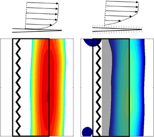




1. Introduction
Trailing edge noise is the dominant noise source of airframe noise in the clean configuration (Lilley Reference Lilley2001). Depending on the nature of the flow past the trailing edge, the noise can include tonal and broadband components. Tonal noise can appear when the boundary layer upstream of the trailing edge is laminar (laminar boundary layer–vortex shedding noise), or when the trailing edge is blunt (trailing edge bluntness–vortex shedding noise) (Brooks, Pope & Marcolini Reference Brooks, Pope and Marcolini1989). If the boundary layer is attached and turbulent, and the trailing edge is sufficiently sharp, then the generated noise is broadband (turbulent boundary layer–trailing edge noise). The primary mechanism of broadband trailing edge noise is edge scattering, which converts the kinetic energy in the turbulent boundary layer to acoustic energy (Ffowcs Williams & Hall Reference Ffowcs Williams and Hall1970; Amiet Reference Amiet1976).
People have known for centuries that an owl's flight is remarkably quiet compared with other birds, and scientists have been studying this phenomenon for over 80 years, starting from Graham (Reference Graham1934). However, there only exist a few quantitative measurements of owl flight noise in the literature. Early measurements (Gruschka, Borchers & Coble Reference Gruschka, Borchers and Coble1971; Kroeger, Grushka & Helvey Reference Kroeger, Grushka and Helvey1972; Neuhaus, Bretting & Schweizer Reference Neuhaus, Bretting and Schweizer1973) did not account for the low flight speed of owls, which is a crucial parameter for the sound level of flow generated noise (Howe Reference Howe2003). Recently, Sarradj, Fritzsche & Geyer (Reference Sarradj, Fritzsche and Geyer2011) performed a field noise measurement of different species of birds, including a Barn Owl. With better acoustic measuring equipment and better control of the flight speed of birds, they found that after minute velocity scaling, the Barn Owl still generates 3–8 dB less flight noise compared with other birds with similar sizes, at frequencies above 1.6 kHz. This critical result proved that owls’ adaptations, apart from the low flight speed, are also responsible for owls’ silent flight. Graham (Reference Graham1934) formally attributed owls’ quiet flying ability to three peculiarities of their plumage: the comb-shaped leading edge serrations, soft trailing edge fringes and velvety upper wing surface. These features became the principal guidelines for subsequent aeroacoustic research. Various methods have been proposed to reduce the trailing edge noise by mimicking these features, as reviewed by Jaworski & Peake (Reference Jaworski and Peake2020). Those methods include trailing edge serrations (Howe Reference Howe1991; Oerlemans et al. Reference Oerlemans, Fisher, Maeder and Kögler2009), trailing edge brush extensions (Herr & Dobrzynski Reference Herr and Dobrzynski2005; Finez et al. Reference Finez, Jondeau, Roger and Jacob2010) and porous trailing edges (Geyer & Sarradj Reference Geyer and Sarradj2014). However, only a limited number of studies focused on the underlying mechanism of the velvety upper wing surface, and currently, there is no application directly based on the velvety structure of owl feathers (Wagner et al. Reference Wagner, Weger, Klaas and Schröder2017).
Several hypotheses have been proposed to explain the function of the velvety structure on owls’ feathers. Graham (Reference Graham1934) postulated that the velvety structure might reduce feather sliding noise when the feathers slide across each other. This hypothesis is highly possible since the velvet length is increased in the feather overlap region (Bachmann et al. Reference Bachmann, Klän, Baumgartner, Klaas, Schröder and Wagner2007; Chen et al. Reference Chen, Liu, Liao, Yang, Ren, Yang and Chen2012). Lilley (Reference Lilley1998) suggested a bypass turbulent cascade mechanism: the thin and compliant filaments in the velvety structures may absorb energy from small-scale turbulent eddies, thus reducing the cutoff frequency of the turbulent cascade process, which corresponds to the Kolmogorov time scale without the presence of velvet structures. There is, however, no experimental proof for this hypothesis. Klän et al. (Reference Klän, Burgmann, Bachmann, Klaas, Wagner and Schröder2012) and Winzen, Klaas & Schröder (Reference Winzen, Klaas and Schröder2014) conducted wind tunnel experiments for wing models covered with artificial velvet structures, with fibre length and density comparable to those of owl wings. They discovered that, at low Reynolds number, the velvet surface was able to delay the flow separation at the suction side of the highly cambered wing. The authors speculated that the reduction of separation contributes to the low flight noise of owls. However, no direct noise measurement was conducted. Clark et al. (Reference Clark, Alexander, Devenport, Glegg, Jaworski, Daly and Peake2016a,Reference Clark, Daly, Devenport, Alexander, Peake, Jaworski and Gleggb) speculated that the velvety structure might lift the boundary layer away from the surface and thus reduce the unsteady wall pressure fluctuation. Clark et al. (Reference Clark, Daly, Devenport, Alexander, Peake, Jaworski and Glegg2016b) applied different porous fabric canopies above a rough surface, and observed that the surface pressure spectrum was significantly reduced by up to 25 dB. This led to a reduction of roughness noise in the mid-frequency of several decibels. They also observed that unidirectional canopies that align with the flow can avoid high-frequency self-noise, but retain the functionality to supress the wall pressure fluctuation. Following these observations, Clark et al. (Reference Clark, Alexander, Devenport, Glegg, Jaworski, Daly and Peake2016a) used finlet fences near the trailing edge to mimic the function of the velvety structure, and observed a noise reduction of up to 10 dB near 3 kHz, at a Reynolds number of  $Re = 3 \times 10^6$, with relatively small adverse aerodynamic effects. Bodling & Sharma (Reference Bodling and Sharma2019) used numerical simulations to confirm that the finlet structures can keep the energetic turbulent structure at the top of the finlets and away from the trailing edge, thereby reducing the effective trailing edge scattering efficiency, especially for small eddies (high frequencies). Afshari et al. (Reference Afshari, Azarpeyvand, Dehghan, Szőke and Maryami2019a) and Afshari, Dehghan & Azarpeyvand (Reference Afshari, Dehghan and Azarpeyvand2019b) used a slightly different noise reduction approach by placing the finlet structures upstream of the trailing edge. These structures can reduce high-frequency components of downstream pressure fluctuations and also the convection velocity. It needs to be mentioned that, although the development of finlet structures stems from the inspiration from owls’ velvet structures, the shape and mechanical properties of those two structures differ significantly.
Some researchers related the porous velvety structure to sound absorption (Chen et al. Reference Chen, Liu, Liao, Yang, Ren, Yang and Chen2012). However, Zhou, Lui & Zhang (Reference Zhou, Lui and Zhang2019a) found that the pure acoustic absorption capability of a thin layer of an owl's velvety structure is negligible, especially near the trailing edge of the wing, where at most two layers of primary feathers can overlap. In addition, as argued by Lilley (Reference Lilley1998), the noise would radiate away with little contact with the wing surface.
There are a few studies that investigated the efficacy of hairy structures (or pile fabrics) in reducing aerodynamic noise. It was observed that hairy structures significantly reduced vortex shedding noise by bluff bodies (Nishimura, Kudo & Nishioka Reference Nishimura, Kudo and Nishioka1999; Nishimura & Goto Reference Nishimura and Goto2010; Kamps et al. Reference Kamps, Geyer, Sarradj and Brücker2017) and vortex interaction noise (Nishimura et al. Reference Nishimura, Kudo and Nishioka1999) by up to 10 dB. The measurements of the wake flow also showed that these hairy structures greatly impacted the turbulent flow and reduced the near-wall velocity gradient over the surfaces of those objects. Nishimura et al. (Reference Nishimura, Kudo and Nishioka1999) studied the impact of pile fabrics on the turbulent boundary layer of a flat plate. They observed that the mean velocity gradient of the turbulent boundary layer above the pile-fabric wall was much reduced compared with that of the smooth case, which was possibly beneficial for noise source reduction. However, no direct noise measurement was performed for this case.
Since biological structures usually possess multi-functionality (Lingham-Soliar Reference Lingham-Soliar2014), it is likely that the velvety structure on owl feathers may contribute to more than one of the above-mentioned functionalities. Up to now, a consensus on the function of the velvety surface has not been achieved, to the understanding of the authors. The aim of the present research is to study the aeroacoustic effects of velvety structures on trailing edge noise through anechoic wind tunnel measurements, combined with theoretical analyses. In the remaining parts of the paper, § 2 describes the set-up of the wind tunnel experiments; § 3 shows the noise and flow measurement results of the baseline flat plate configuration and several coated configurations; § 4 proposes a theoretical model to relate the flow and noise measurements, based on which discussions are made on the aeroacoustic functionalities of velvety structures; § 5 gives a summary.
2. Experimental set-up
2.1. Fabrication of artificial velvet structure
Motivated by the velvety structures of owls’ feathers, three different types of velvety coatings with varying hair dimensions and number densities were fabricated, as shown in table 1. The velvety coating contains nylon fibres with a Young's modulus of 2.5–3.9 GPa. However, as the fibre diameter is larger than that in an owl's velvet structure, the artificial velvet structure is more rigid than the real velvety structure. The fibres were attached to a 0.05 mm thick polyethylene terephthalate substrate film perpendicularly through the electrostatic flocking technique. The coated film was then cut and adhered to the flat plate model on both sides. Figure 1 shows microscopic images of the real velvet structure of an owl's feather and an artificial velvety coating with 1mm thickness (H1.0). Most of the fibres are nearly perpendicular to the surface in the artificial velvet coating. Several (rigid) smooth coatings made of polypropylene sheet were also used in this experiment for comparison. The parameters of these coatings are shown in table 1. The purpose of testing these smooth coatings is to indicate the effect of changing the external shape and the trailing edge thickness of the baseline flat plate model.
Parameters of the artificial velvety coatings and smooth coatings.

(a) The velvety structure of an eagle owl feather under a scanning electron microscope. (b) A photo of a 1mm-thick velvety coating (H1.0) under an optical microscope.

2.2. Anechoic wind tunnel facility
The trailing edge noise measurements and flow measurements were conducted in an anechoic wind tunnel, ultra-quiet noise injection test and evaluation device (UNITED) (Zhou et al. Reference Zhou, Sun, Fattah, Zhang and Huang2019b; Bu, Huang & Zhang Reference Bu, Huang and Zhang2020), at The Hong Kong University of Science and Technology. The open-jet test section was used for this study. The nozzle of the wind tunnel has a square cross-section with a side length of 0.4 m. The flow speed can vary from 10 to 70 m s $^{-1}$, and the inflow turbulence intensity is lower than 0.27 % within the speed range of 16–30 m s $^{-1}$. The test section is enclosed by an anechoic chamber with a cutoff frequency of 200 Hz. Dimensions of the chamber are 3.3 m (length) $\times$ 3.1 m (width) $\times$ 2.0 m (height).
2.3. Flat plate model
A flat plate model was used in this study to simplify the flow condition. The model has a chord of 150 mm, a span of 400 mm and a thickness of 6 mm. The cross-sectional geometry of the model is shown in figure 2(a). The model has an elliptical leading edge with an aspect ratio of 4 : 1 and a symmetric trailing edge with a contraction angle of 12 $^\circ$. The thickness at the trailing edge is measured to be less than 0.2 mm. A fillet with a 500 mm radius was added between the flat section and the contraction section of the model to prevent flow separation, which typically occurs for a bevelled type trailing edge (Doolan et al. Reference Doolan, Tetlow, Moreau and Brooks2012). Two acrylic endplates were used to hold the flat plate model to maintain two-dimensionality of the flow and to prevent the noise associated with a free shear layer. The angle of attack of the flat plate was set as 0 $^\circ$. In this work, the centre of the trailing edge is set as the origin; $+x$ represents the streamwise direction; $+y$ represents the direction normal to the chord and towards the phased microphone array; and $+z$ represents the vertical direction pointing upwards. To suppress the laminar boundary layer instability noise, a serrated trip strip with a thickness of 0.3 mm was attached to both sides of the model, occupying a 12 % to 20 % portion of the chord. The free-stream velocity $U_0$ in this experiment ranges between 16 and 30 m s $^{-1}$, corresponding to a chord-based Reynolds number between $1.6 \times 10^5$ and $3.0 \times 10^5$. These velvet/smooth coatings, as introduced in § 2.1, were placed just downstream of the trip strips and had a chordwise coverage from 20 % to 100 % (i.e. $-120 \leq x \leq 0$ mm). The span of the coatings was the same as that of the flat plate model.
The set-up of the wind tunnel experiment. (a) The dimensions of the cross-section of the flat plate model. All numbers are in millimetres. (b) The acoustic measurement set-up, including the endplates, the flat plate model with velvety coating and the phased microphone array.

2.4. Phased microphone array measurement
Figure 2(b) shows the planar phased microphone array used to acquire the sound source distribution in this study. It consists of 56 1/4 inch Brüel & Kjær type 4957 microphones. Each microphone has a flat frequency response within 50 to 10 000 Hz, and was calibrated by a Brüel & Kjær type 4231 sound calibrator. The microphones are located in 7 spiral arms to reject spatial aliasing (Huang Reference Huang2011). The microphone plane was set vertical and parallel to the flow direction with a distance of 0.728 m from the flat plate trailing edge, and the centre of the microphone array was aligned with the centre of the trailing edge of the flat plate. Four 24-bit National Instrument PXIe-4497 cards were used to record the microphone data simultaneously. The sampling frequency was 48 kHz, and the number of data points per channel for each measurement was 409 600.
Fast Fourier transformation was used to transform the data into the frequency domain. The data were divided into 199 Hanning windows with a window size of 4096 and 50 % overlap, resulting in a frequency resolution of 11.72 Hz. The cross-spectral matrix was obtained by averaging the cross-spectra of the 199 blocks. The conventional beamforming algorithm with diagonal removal was used to calculate the source distribution within the model plane.
Because of the distributed nature of the trailing edge noise, a source integration method with an array calibration function (ACF) was used to quantify the absolute trailing edge noise strength (Brooks & Humphreys Reference Brooks and Humphreys1999). Several simulated single-frequency line sources distributed along the trailing edge were constructed. The source at each grid point was set to be uncorrelated, which is representative of trailing edge noise (Oerlemans & Sijtsma Reference Oerlemans and Sijtsma2002). The ACF is then defined by (2.1)
 \begin{equation} {ACF} = {SPL_{integrated}} -{ SPL_{actual}},\end{equation}
where  ${SPL_{actual}}$ is defined as the sound pressure level measured by a microphone located at the centre of the microphone array, and ${SPL_{integrated}}$ is the integrated source strength within the integration region. The integration region is centred at the centre of the trailing edge and has a size of 3/2 chord $\times$ 1/4 span. The purpose is to exclude other unwanted sound sources, such as the model–endplate junction noise and jet collector noise, but to include potential contributions from the velvety coatings. After the correction by (2.1), it was found that the size of the integration region does not affect the measured noise level of the flat plate model. In addition, although the microphone array has a deteriorated resolution at low frequency, this integration method produces almost the same sound level as the time-domain delay-and-sum method below 800 Hz. Therefore, the low-frequency limit of the acoustic measurement is chosen at 200 Hz, which is the cutoff frequency of the anechoic chamber. The high-frequency limit of the acoustic measurement is chosen at 10 000 Hz, which is the upper limit of the microphone.
2.5. Hot-wire anemometry
Hot-wire anemometry was used to acquire the velocity profile as well as the turbulence characteristics of the boundary layer in the vicinity of the trailing edge. A Dantec type 55P11 single-sensor hot-wire probe and a Dantec StreamLine Pro Anemometer System were used. The probe was calibrated by the Dantec StreamLine Pro Automatic Calibrator within the speed range of 0 to 30 m s $^{-1}$ before being installed into the wind tunnel. A Dantec traverse system with a positional accuracy of 6.25 $\mathrm {\mu }$m was used to position the probe in the test section. The probe was placed at the mid-span location and had a streamwise distance of 0.7 mm from the flat plate trailing edge ( $x = 0.7$ mm, $z = 0$ mm). A closer distance was not attempted to avoid potential damage to the hot-wire probe. The direction of the hot-wire is parallel to the trailing edge, which enables maximal spatial resolution in the chord-normal direction. The set-up is shown in figure 3. For each measurement, the probe scanned across the wake within $y = \pm 15$ mm, with a step size of 0.2 mm. Velocities were sampled at a frequency of 50 000 Hz with a sampling time of 8 s. For spectrum calculation, the data were divided into 159 Hanning windows with a window size of 5000 and an overlap ratio of 50 %. This leads to a frequency resolution of 10 Hz.
The experimental set-up for hot-wire anemometry. (a) Overall layout. (b) Close-up view for the near-wake measurement.

3. Experimental results
3.1. Baseline measurement
3.1.1. Acoustic measurement
Figure 4 shows some typical sound maps of the flat plate model and the background. The sound map has already been integrated within a 1/3 octave range to reduce statistical fluctuation. It is clear that, above 2000 Hz, the major noise sources from the flat plate model are located along the trailing edge. In terms of the background noise, at low frequencies, the major noise source is from the nozzle (on the left) and the jet collector (on the right); at higher frequencies (4000 Hz and 8000 Hz), the noise emitted from the trailing edges of the endplates is visible. However, it is clear that in the integration region, the level of trailing edge noise source is much larger than the background noise (by at least 10 dB), indicating that the beamforming method is effective in isolating the trailing edge noise from the background noise.
The 1/3 octave sound maps of the flat plate model (left column) and the background (right column) at three different frequencies at  $U_0 = 20$ m s $^{-1}$. The solid rectangle in the middle represents the flat plate model, and the dotted-line rectangle represents the source integration region. The left grey rectangle and the two grey lines denote the wind tunnel nozzle and the endplates, respectively. The dynamic range of each plot is 12 dB.

The comparison between the flat plate trailing edge noise and the background noise is shown in figure 5. The reason that the background noise at several kHz is out of range is that, after diagonal removal, the conventional beamforming method can give a negative source distribution at some non-source regions, and the negative source intensity was set to zero. But even though the background noise within the integration region may be underestimated at these frequencies, it is still evident that the signal to noise ratio exceeds 10 dB. Therefore, the effect of background noise can be neglected except at low frequencies. The theoretical prediction based on the flat plate assumption by Amiet (Reference Amiet1978) and the empirical boundary layer statistics (Goody Reference Goody2004) is also plotted as a reference in figure 5. The fluctuation in the predicted spectrum at  $90^\circ$ is due to the finite chord length of the model (Amiet Reference Amiet1978) and is independent of the flow speed. Since the diameter of the microphone array is not negligible with respect to the observation distance, it is necessary to take the average between the observation angles. The weighted average considering the distribution of the microphone observation angles is used here. This takes into account the effect that more microphones are located near the $90^\circ$ observation angle. This is compared with the simple averaging method, which assumes a uniform microphone distribution within the observation angle limits. After the averaging process, the fluctuation in the prediction is largely suppressed, and the theoretical prediction is in reasonable agreement with the measured spectrum. However, there is an underprediction at mid-to-high frequencies, which is likely caused by the inaccuracy of Goody's wall pressure spectrum for this case. A better prediction using the near wake turbulent statistics as input will be presented in § 4.2.
The flat plate trailing edge noise, the background noise and the theoretical predictions at two different free-stream velocities. The red dashed curve represents the predicted sound level at a  $90^\circ$ observation angle. The thin dashed blue line and solid blue line represent the simple average and weighted average of the predicted noise within the observation angle of the microphone array, respectively.

The trailing edge noise of the baseline tripped flat plate model was measured twice with a six-month interval. Between these two measurements, there were many other experiments conducted in the wind tunnel, and the set-up of the wind tunnel changed continuously. Nevertheless, the average difference in terms of the power spectral density (PSD) in the range 200–10 000 Hz was 0.37 dB at 20 m s $^{-1}$ and 0.02 dB at 30 m s $^{-1}$, respectively. Therefore, the repeatability of the spectral measurement is estimated to be within 0.4 dB.
3.1.2. Near-wake flow measurement
Figure 6 shows the distribution of the mean streamwise velocity  $U$ and the root mean square fluctuating component $u_{rms}$ at the near wake of the flat plate model ( $x = 0.7$ mm) at $U_0 = 20$ m s $^{-1}$. It can be used to reveal the boundary layer properties in the upstream vicinity of the trailing edge. First, the flow is fully attached at the trailing edge, indicating that the smooth geometrical transition between the flat part and the trailing edge part was effective. Secondly, the symmetrical shape of the mean velocity distribution confirms that the install angle was $0^\circ$.
The distribution of (a) the mean velocity  $U$ and (b) the velocity fluctuation $u_{rms}$ in the near wake of the flat plate model. Here, $U_0 = 20$ m s $^{-1}$.

Assuming that the near-wake velocity distribution is the same as the boundary layer velocity distribution just ahead of the trailing edge, we can estimate the boundary layer statistics, including the boundary layer thickness  $\delta$, displacement thickness $\delta ^*$ and the momentum thickness $\delta _\theta$, as shown in table 2. The values in the table are the averages of the boundary layers on two sides. The empirical value (Schlichting & Gersten Reference Schlichting and Gersten2016) and the prediction by the program XFOIL (Drela Reference Drela1989) are also shown as a comparison. The measured $\delta ^*$ and $\delta _\theta$ are close to the XFOIL prediction, but higher than the empirical value. This is due to the slight adverse pressure gradient upstream of the trailing edge. The discrepancy between the measured and predicted $\delta$ will be explained in § 4.2.
The boundary layer thickness  $\delta$, displacement thickness $\delta ^*$ and the momentum thickness $\delta _\theta$ at the trailing edge. The near-wake velocity distribution was assumed to be the same as the boundary layer velocity distribution. Here, $U_0 = 20$ m s $^{-1}$.

The spectral information of the turbulent wake of the flat plate is shown in figure 7. The broadband feature of the spectrum also confirms a successful transition by the trip strip. The majority of the turbulent kinetic energy is concentrated within the boundary layer and at low frequencies. In order to characterize the overall turbulent energy distribution within the whole boundary layer, integration of the turbulent spectrum was conducted in the chord-normal direction ( $y$-direction) and is shown in figure 8
 \begin{equation} {PSD_{u, overall}} = \int_{{-}H/2}^{H/2} {PSD_{u}} \, \mathrm{d} y , \end{equation}
where H is the length of integration and  $H/2>\delta$ is required to capture the entire boundary layer. In the overall spectrum, there is an energy-containing range at low frequency and an inertial subrange following the $-$5/3 law between 2000 and 10000 Hz.
The spectrum of  $u$ in the near wake of the flat plate. Here, $U_0 = 20$ m s $^{-1}$.

The integrated velocity spectrum of  $u$ in the near wake of the flat plate along the transverse direction. Here, $U_0 = 20$ m s $^{-1}$.

3.2. Effect of velvety coating on noise and flow
3.2.1. Noise measurement
Figure 9 shows the narrow band trailing noise spectra corresponding to different velvety coatings and smooth coatings. The 1/3 octave spectra, shown in figure 10, have less fluctuation compared with the narrow-band spectra. The effect of velvety coatings on the trailing edge noise is largely frequency dependent. In general, for each velvety coating at a certain flow speed, there is a cross-over frequency  $f_{c}$, below which the coating increases the trailing edge noise, while above $f_{c}$, the trailing edge noise is reduced. The noise increase in the low-frequency range has a hump-like shape, and the noise reduction at high frequencies is broadband. Due to the upper limit of the frequency response of the microphones, the effect of the velvety coating at frequencies above 10 000 Hz was not determined. From the trend of the spectrum, it is conjectured that the noise increase by the coating occurs at some frequency beyond 10 000 Hz. The hair dimension affects both the cross-over frequency and the magnitude of noise increase/reduction. For example, compared with other velvety coatings, the coating H1.5 gives a lower $f_{c}$, and a higher noise reduction for most of the frequencies above $f_{c}$. However, it also gives a higher noise increase in the low-frequency range.
The noise spectra in the trailing edge region for flat plates covered with different coatings.

The 1/3 octave spectra in the trailing edge region for flat plates covered with different coatings.

As a comparison, smooth coatings lead to additional tonal noise. The trailing edge thickness-based Strouhal number  $St_h = f h/U_0$ for the tonal peak is around 0.15, which is similar to the results for the blunt trailing edge vortex shedding noise in the study by Brooks et al. (Reference Brooks, Pope and Marcolini1989), where $St_h$ lies between 0.12 and 0.2 for an aerofoil with plate extensions. The noise level at frequencies below the vortex shedding frequency is not affected by the presence of a smooth coating. This indicates that the mechanism for the low-frequency hump caused by the velvety coating is not due to vortex shedding. More details on the mechanism will be given in § 4. Smooth coatings also lead to a broadband noise reduction at high frequency. However, the magnitude is not as high as that of the velvety coating of the same thickness. For example, at 20 m s $^{-1}$, the maximum noise reduction by the H1.5 velvety coating is 18 dB, while it is 9 dB for the S1.5 coating.
Figure 11 shows the normalized 1/3 octave spectra at free-stream speeds between 16 and 30 m s $^{-1}$. The frequency is normalized to the chord-based Strouhal number $St = f c/U_0$. A reasonable collapse is achieved with a velocity scaling of $U_0^5$ except for the tonal peaks, which is consistent with the classical trailing edge noise theory (Ffowcs Williams & Hall Reference Ffowcs Williams and Hall1970). Figure 12 shows the change of the sound spectrum caused by the coating compared with the baseline flat plate case. A positive ${\rm \Delta} PSD$ represents a noise increase, and vice versa. All measurement results with a free-stream velocity between 16 m s $^{-1}$ and 30 m s $^{-1}$ are plotted. To reduce the fluctuation in the spectrum, a robust locally weighted regression (RLOWESS) filter (Cleveland Reference Cleveland1979) with a window size of 30 was applied to smooth the data. After data smoothing, the change of trailing edge noise ${\rm \Delta} PSD$ caused by the coating is found to be a quantity achieving good data collapse, especially when the frequency is close to $f_{c}$ or beyond $f_{c}$. This data collapse indicates the underlying mechanism for noise reduction remains the same within the measured flow speed range. The cross-over Strouhal number $St_{c}$ corresponding to $f_{c}$ appears to be nearly invariant within the measured speed range; $St_{c}$ is negatively related to the length of the velvety coating. For the velvety coatings, the magnitude and central frequency of the low-frequency hump do not collapse well with Strouhal number. As flow speed increases, the magnitude of the hump increases, while the central frequency of the hump decreases. This indicates that the disturbing effect of the velvety coating is larger at high speed, while the corresponding length scale is smaller. For the smooth coating, the central Strouhal number of the vortex shedding tone is nearly constant, indicating a speed-independent length scale. The magnitude of the tone increases with the incoming flow speed.
The scaled 1/3 octave spectra as a function of chord-based Strouhal number  $St$ for flat plates covered with different coatings. The sound level is scaled with $U_0^5$.

The relationship between  ${{\rm \Delta} PSD}$ and the chord based Strouhal number $St$, with data smoothed by a RLOWESS algorithm. The corresponding $U_0$ is between 16 and 30 m s $^{-1}$. A positive ${{\rm \Delta} PSD}$ represents a noise increase.

The sound maps are then used to reveal the location of the major noise sources. First, the origin of the low-frequency hump is investigated. Since the array resolution is better at a higher frequency, the sound maps of the baseline configuration and the H0.3 configuration are compared at 2000 Hz and 30 m s $^{-1}$. Although this frequency is not at the centre of the low-frequency hump, at this condition, ${{\rm \Delta} SPL}$ still exceeds 7 dB. Figure 13 shows that the major noise sources for the coated model are distributed along the trailing edge, and the magnitude is increased compared with the reference case. This indicates that the noise source for the low-frequency hump is at the trailing edge, even if the trailing edge is covered by the velvety coating.
The 1/3 octave sound maps at 2000 Hz for (a) the flat plate configuration and (b) the H0.3 configuration. Here,  $U_0= 30$ m s $^{-1}$.

Next, the high-frequency noise reduction by the velvety coating is studied. The sound maps of the baseline configuration, H0.3 configuration, H1.5 configuration and S1.5 configuration are compared at 5000 Hz at 20 m s $^{-1}$ in figure 14. The corresponding ${{\rm \Delta} SPL}$ are $-9$ dB (H0.3), $-17$ dB (H1.5), $-9$ dB (S1.5), respectively. These coatings all reduce the noise source level at the central trailing edge position. It is interesting to notice that, for the H0.3 and S1.5 configurations, the dominant noise source is still distributed along the trailing edge, while for the H1.5 case, the major noise sources are at the wind tunnel nozzle and the plate–endplate junction. A direct comparison between the H1.5 and S1.5 configurations shows a superior noise reduction potential by the velvety coating, at the same coating thickness.
The 1/3 octave sound maps at 5000 Hz for (a) the flat plate configuration, (b) the H0.3 configuration, (c) the H1.5 configuration and (d) the S1.5 configuration. Here,  $U_0= 20$ m s $^{-1}$.

3.2.2. Near-wake flow measurement
The mechanism of the noise spectrum modification was investigated through the measurement of the near-wake flow. The distributions of mean velocity  $U$ and fluctuating velocity $u_{rms}$ are plotted in figure 15, and the spectral information is plotted in figure 16. It is clear that the velvety coatings broaden the boundary layer compared with the baseline configuration. The thicker velvety coatings have a larger effect on boundary layer broadening. In contrast, smooth coatings do not significantly increase the boundary layer thickness. This indicates the broadening effect by the velvety coatings is probably linked to their surface structure. For thicker coatings, there exists a region near $y=0$ where both mean velocity and fluctuating velocity are small. This is related to the bluntness caused by these coatings. For smooth coatings, we can see a large velocity gradient near the offset wall, similar to the baseline case. For the cases of velvety coatings, the near-wall velocity gradient is much reduced, which is consistent with the observation by Nishimura et al. (Reference Nishimura, Kudo and Nishioka1999). Similarly, in another study on porous aerofoils, Geyer & Sarradj (Reference Geyer and Sarradj2014) reported that, compared with non-porous aerofoils, porous aerofoils lead to a thicker boundary layer (up to three times the original boundary layer thickness) and smaller near-wall velocity gradient. In terms of the fluctuating velocity component, the velvety coatings widen the regions with high velocity fluctuations, and thicker velvety coatings have a larger effect. In contrast, the smooth coatings do not widen the region with high fluctuating velocity. Instead, the major effect is to offset the turbulent boundary layer outwards by approximately the thickness of the coating.
The distribution of (a) the mean streamwise velocity  $U$ and (b) the root-mean-square (r.m.s.) fluctuating velocity $u_{rms}$. Here, $U_0= 20$ m s $^{-1}$.

The spectral density of the fluctuating velocity component  $u$ at different chord-normal locations $y$. Here, $U_0= 20$ m s $^{-1}$.

The spatial distributions of the streamwise velocity fluctuation spectrum of several configurations are plotted in figure 16. It is clear that all spectra have a broadband component, which confirms that the flow at the trailing edge is turbulent. The turbulent energy is dominated by low-frequency components and is concentrated within the boundary layer. For the H0.3 and H1.5 configurations, there are three major differences from the clean configuration. First, the width of the region with high velocity spectrum is increased. Second, there is a wider region of low velocity spectrum around  $y = 0$. It is clear that the high-frequency velocity fluctuation is reduced in this central zone, compared with the clean configuration. The increased width of this region can be attributed to the increased trailing edge bluntness caused by the coating. Third, at the outer region of the boundary layer, a broadband hump is visible. The central frequency for the hump is 1000 Hz for the H0.3 configuration and 500 Hz for the H1.5 configuration. These two frequencies match with the broadband hump in the corresponding noise spectra. For the smooth coating S1.5, the broadband spectrum is similar to the baseline configuration, except that the turbulent structure is approximately offset outward by the thickness of the coating. A significant tonal peak at 1 kHz and its harmonics are visible, suggesting vortex shedding behind the blunt trailing edge. However, vortex shedding is not present for all the velvety coating configurations. The possible mechanism is that the velvety structures can destroy the spanwise coherence of the boundary layer structures and suppress vortex shedding, as is the case with a porous surface (Ali, Azarpeyvand & da Silva Reference Ali, Azarpeyvand and da Silva2018).
The overall velocity spectra  ${PSD_{u, overall}}$ under different configurations are plotted in figure 17. The calculation method was introduced in § 3.1.2. The velvety coatings consistently elevate the integrated turbulent spectrum within the whole frequency range, and the thicker coatings lead to a larger increase. The increase is more prominent in the low-frequency range. No tonal peak related to vortex shedding is detected for the velvet configurations. In contrast, the smooth coatings do not significantly change the broadband level of ${PSD_{u,overall}}$, but only add several tonal peaks to the spectra. These spectral peaks are directly related to vortex shedding behind the blunt trailing edge. Therefore, the increase of the velocity spectra by the velvety coatings is likely attributed to their extra surface roughness. It is counter-intuitive that, although the velvety coatings significantly elevate the overall high-frequency turbulent energy, they can still reduce more high-frequency noise compared with the smooth coating of the same thickness. This will be discussed in detail in § 4.2.
The integrated velocity spectrum of  $u$, defined in (3.1), under different configurations. Here, $U_0= 20$ m s $^{-1}$.

3.3. Further study on the effect of velvet locations
In § 3.2, all the coatings cover the original sharp trailing edge of the flat plate model, which modifies the bluntness of the trailing edge. In this section, two additional configurations are tested to further reveal the noise modification mechanisms. In ‘H1.0,  $[-120\ -65]$’, the H1.0 velvet coatings cover the chordwise region $-120\ \mathrm {mm} \leq x \leq -65\ \mathrm {mm}$ on both sides of the flat plate, and in ‘H1.0, $[-55\ 0]$’, the H1.0 velvet coatings cover the chordwise region $-55\ \mathrm {mm}\leq x \leq 0\ \mathrm {mm}$. In the former set-up, the velvet coatings do not cover the trailing edge, leading to a sharp trailing edge, and in the latter set-up, the trailing edge is covered by velvet structures.
Figure 18 summarizes the effect of velvet locations on the noise spectra and near-wake flow. Interestingly, the ‘H1.0,  $[-55\ 0]$’ configuration leads to almost the same noise spectrum as the original H1.0 configuration. In comparison, the ‘H1.0, $[-120\ -65]$’ configuration gives almost no high-frequency noise reduction, but still produces significant low-frequency noise increase. From figure 18(b,c), it can be observed that the ‘H1.0, $[-55\ 0]$’ configuration gives similar near-wake flow characteristics as the H1.0 configuration, but the ‘H1.0, $[-120\ -65]$’ configuration gives a very different distribution. The boundary layer as well as the high turbulence region of ‘H1.0, $[-120\ -65]$’ are broadened compared with the flat plate, due to the presence of velvet structures upstream of the trailing edge. However, the near-wall velocity gradient and turbulence distribution resemble that of the flat plate. This indicates the near-wall flow structures might be closely linked to the high-frequency noise generation. Lastly, figure 18(d) shows that all the velvety coatings, despite the chordwise locations, significantly elevate the turbulent energy level within the boundary layer at all frequencies. Further discussion on the relation between near-wake flow and sound generation will be provided in § 4.2.
The effect of velvet location on the (a) sound spectra, (b) mean velocity distribution at the near wake, (c) r.m.s. velocity distribution at the near wake and (d) the integrated velocity spectra of  $u$, defined in (3.1).

4. Mechanisms of the noise modification by velvety coatings
4.1. The effect of trailing edge geometry
Most trailing edge noise theories assume a sharp trailing edge. For example, the initial development of trailing edge noise formulation by Ffowcs Williams & Hall (Reference Ffowcs Williams and Hall1970) assumed the aerofoil to be a semi-infinite plate with zero thickness. Later development by Amiet (Reference Amiet1976) and Roger & Moreau (Reference Roger and Moreau2005) took a finite chord into consideration, but still assumed the trailing edge to be infinitely sharp. In the semi-empirical self-noise prediction model developed by Brooks et al. (Reference Brooks, Pope and Marcolini1989), the trailing edge bluntness was only considered in the blunt trailing edge vortex shedding noise and was considered unrelated to the turbulent boundary layer trailing edge noise. Although in a comprehensive experimental study, Herr (Reference Herr2007) showed that the trailing edge bluntness significantly modifies the broadband noise at frequencies above the vortex shedding frequency, currently, few researchers consider the bluntness effect on the turbulent boundary layer trailing edge noise.
To the authors’ knowledge, the study by Howe (Reference Howe1988, Reference Howe1999, Reference Howe2000) was the only theoretical analysis of the effect of trailing edge shape on turbulent boundary layer trailing edge noise. His analysis was based on the theory of vortex sound (Howe Reference Howe2003) and did not consider the vortex shedding due to trailing edge bluntness and the corresponding noise radiation. The factors including finite trailing edge thickness, trailing edge geometry and the trailing edge flow topology were shown to have a large impact on the trailing edge scattering process and noise generation. The theoretical model by Howe (Reference Howe2000) took the wavenumber–frequency spectrum of the blocked wall pressure as input to predict the far-field trailing edge noise. The key results of this generalized theory are summarized here and will be applied to the trailing edges used in this experiment.
4.1.1. Theoretical formulation
The basic formulation in Howe's model is about the scattering of a vortex past through a blunt trailing edge, as shown in figure 19. A rectangular-shaped trailing edge is used to match with the experimental set-up. The thickness  $h$ is equal to twice the coating thickness. Since sharp separation occurs at the blunt trailing edge, it is assumed that the trajectory of the vortex is fully separated, i.e. parallel to the undisturbed mean flow direction. The magnitude of the vortex is assumed to be invariant along its trajectory under the frozen turbulence assumption (Taylor Reference Taylor1938). The flow elsewhere is assumed to be potential.
The formulation of the scattering problem of a single vortex past a rectangular trailing edge. The region outside the rectangular aerofoil in the  $z$-plane is mapped to the upper half-plane in the $\zeta$-plane.

The two-dimensional (2-D) potential flow assumption enables the analysis using conformal mapping. The region outside the rectangular aerofoil in the  $z$-plane ( $z = x + \textrm {i} \,y$) is mapped to the upper half-plane in the $\zeta$-plane ( $\zeta = \eta + \textrm {i} \,\xi$). Note that the symbol $z$ here is a complex number and does not represent the spanwise location. This is achieved by the following transformation:
 \begin{equation} \frac{z}{h} = f(\zeta)={-}\frac{1}{\rm \pi}\{\zeta \sqrt{\zeta+1}\sqrt{\zeta-1}-\ln (\zeta +\sqrt{\zeta+1} \sqrt{\zeta-1})\}-\frac{\textrm{i}}{2}. \end{equation}
 Vortex sound is generated only if the vortex moves across the streamlines of ideal incompressible flow around the trailing edge (Howe Reference Howe2003), as illustrated in figure 20. After being transformed into the  $\zeta$-plane, these streamlines correspond to a uniform flow along the $+\eta$ direction. For an infinitely thin trailing edge, the velocity potential is
 \begin{equation} \varphi^*(x,y) = \sqrt{r} \sin (\theta/2), \end{equation}
where  $(x, y ) = (r \cos \theta , r \sin \theta )$, $r$ is the distance between the observer and the trailing edge and $\theta$ is the observation angle with the downstream direction set as zero. For a rectangular-shaped trailing edge with a thickness of $h$, the streamlines near the blunt edge is different from that of the sharp case. However, the velocity potential approaches $\varphi ^*(x,y)$ far from the trailing edge. Denoting the velocity potential around the blunt edge by $\varPhi ^*(x,y)$, then
 \begin{equation} \varPhi^*(x,y) \to \varphi^*(x,y) \text{ as } \sqrt{x^2+y^2} \to \infty . \end{equation}
Here,  $\varPhi ^*$ can then be represented as a function of $\zeta$ by
 \begin{equation} \varPhi^* \equiv \varPhi^*(z) ={-} \mu\, Re \,\zeta, \quad \mu > 0 , \end{equation}
where  $\mu$ is a constant coefficient to ensure the condition in (4.3). The main result from Howe's model is that, for the same incoming turbulent wall pressure fluctuation that is convected by a speed $U_c$, the effect of trailing edge shape on the far-field acoustic pressure spectrum can be represented using a factor $|\mu \mathcal {I}(\omega /U_c)|^2$, where
 \begin{equation} \mathcal{I}(k_1) =
\mathcal{I}\left(\frac{\omega}{U_c}\right) = \begin{cases}
\displaystyle \left(\textrm{e}^{{-}k_1 h /2}
\int_{-\infty}^{\infty} \textrm{e}^{-\textrm{i} k_1 z}\,
\mathrm{d} \zeta\right)^*, & \text{if } k_1 \geq 0,\\
-(\mathcal{I}({-}k_1))^*, & \text{if } k_1 < 0,
\end{cases} \end{equation}
\begin{equation} \mathcal{I}(k_1) =
\mathcal{I}\left(\frac{\omega}{U_c}\right) = \begin{cases}
\displaystyle \left(\textrm{e}^{{-}k_1 h /2}
\int_{-\infty}^{\infty} \textrm{e}^{-\textrm{i} k_1 z}\,
\mathrm{d} \zeta\right)^*, & \text{if } k_1 \geq 0,\\
-(\mathcal{I}({-}k_1))^*, & \text{if } k_1 < 0,
\end{cases} \end{equation}
where  $\omega$ is the angular frequency, $k_1$ is the streamwise hydrodynamic wavenumber and the asterisk denotes the complex conjugate. When the frequency of interest is very low, or when the trailing edge is very thin, the domain can be viewed as a half-plane such that
 \begin{equation} \mu\mathcal{I}\left(\frac{\omega}{U_{c}}\right) \sim \mu\mathcal{I}_0 \left(\frac{\omega}{U_{c}}\right) = \mathrm{e}^{-\mathrm{i} {\rm \pi}/ 4} \sqrt{\frac{{\rm \pi} U_{c}}{\omega}}, \quad \frac{\omega h}{U_{c}} \ll 1 . \end{equation}
The streamlines (thin grey lines) of an ideal incompressible flow around a trailing edge (thick black lines): (a) rectangular trailing edge with a thickness  $h$; (b) infinitely thin trailing edge.

Therefore, we can represent the effect of reduced scattering efficiency of a finite-thickness trailing edge compared with the ideal zero-thickness trailing edge by
 \begin{equation} {{\rm \Delta} SPL_{th}} = 20 \log \left| \frac{\mathcal{I}(\omega/U_c)}{\mathcal{I}_0(\omega/U_c)} \right| . \end{equation}
 The above analysis assumes a semi-infinite aerofoil and thus does not account for the effect of leading edge back scattering on trailing edge noise (Roger & Moreau Reference Roger and Moreau2005). However, it can be argued that  ${{\rm \Delta} SPL_{th}}$ remains the same in the case of a finite chord, since the leading edge has no effect on the hydrodynamic field at the trailing edge, and the back-scattered sound intensity is proportional to the sound generated directly at the trailing edge. For completeness, the detailed derivation of the results can be seen in Appendix A.
4.1.2. Comparison with experimental results
It is straightforward to use numerical integration to evaluate the effect of  ${{\rm \Delta} SPL_{th}}$, as shown in figure 21. The convection velocity $U_c$ is set to be 0.7 times the free-stream velocity $U_0$ in the calculation (Roger & Moreau Reference Roger and Moreau2004). For a trailing edge thickness-based Strouhal number $St_h <10^{-2}$, the thickness has almost no effect on the scattering efficiency, and the trailing edge can be regarded as sharp. As $St_h$ increases, the reduction of ${{\rm \Delta} SPL_{th}}$ first comes from the reduction of pressure fluctuation at the lower side of the aerofoil by a factor of $\exp (-k h)$. At $St_h>1$, the contribution from the lower side of the aerofoil to trailing edge noise can be neglected, and the noise is only caused by the scattering of boundary layer turbulence by a right-angled wedge.
The prediction of the change of turbulent boundary layer-trailing edge noise due to the bluntness effect,  ${{\rm \Delta} SPL_{th}}$, (a) as a function of trailing edge thickness-based Strouhal number $St_{h}$; and (b) as a function of frequency at $U_0 = 20$ m s $^{-1}$. The measurement results are shown for comparison for the latter case.

The measured noise reduction level is also plotted for comparison. The noise increase in the experiment below the critical frequency is caused by other mechanisms, as discussed in § 3.2.1. The prediction is consistent with the observation that the addition of smooth coating only slightly modifies the low-frequency noise (below vortex shedding frequencies), and the trend in the mid- to high-frequency range is qualitatively consistent with the experiment. However, it does not predict a correct  ${{\rm \Delta} SPL_{th}}$ value for both velvety coatings and smooth coatings at high frequencies, suggesting that there could be additional reasons for the large modification of the noise spectrum apart from the bluntness effect. In the above analysis to calculate ${{\rm \Delta} SPL_{th}}$, we made the assumption that the spectrum of the fluctuating wall pressure is not altered. This is not necessarily true in the experiment, and the effect of coatings on the wall pressure spectrum will then be discussed in § 4.2.
4.2. The effect of turbulent boundary layer characteristics
In this experiment, due to the small thickness of the flat plate model and the presence of coatings, direct measurement of the wall pressure spectrum was not conducted. However, it is possible to estimate the wall pressure spectrum from the boundary layer characteristics based on the method developed by Blake (Reference Blake1986). The method was applied to the prediction of aerofoil trailing edge by Parchen (Reference Parchen1998) from the Netherlands Organisation for Applied Scientific Research (TNO), and it is therefore known as the TNO-Blake model. A recent extension of the model was conducted by Stalnov, Chaitanya & Joseph (Reference Stalnov, Chaitanya and Joseph2016). This prediction scheme is more generic than other semi-empirical models. For example, it was used to analyse the effect of the aerofoil shape on trailing edge noise by Lee (Reference Lee2019). Key steps of the TNO-Blake model will be briefly introduced here for completeness. A new model based on the TNO-Blake model and Howe's model will be used to predict the trailing edge noise of both the baseline and coated configurations. The model uses the measured near-wake distribution of mean and fluctuation velocities as input.
4.2.1. Theoretical formulation
In the following, for notational convenience, we use  $\boldsymbol {x} = (x_1, x_2, x_3)$ to represent the spatial coordinate, where the subscripts 1, 2 and 3 represent the streamwise, wall-normal and spanwise directions, respectively. Blake (Reference Blake1986) derived the turbulent wall pressure fluctuation $p'$ as a solution of Poisson's equation, with the source term $\mathcal {S}$
 \begin{equation} \frac{\partial^{2} p^{\prime}}{\partial x_{i} \partial x_{i}} ={-}\mathcal{S}={-}\mathcal{S}^{M S}-\mathcal{S}^{T T} , \end{equation}
where
 $$\begin{gather} \mathcal{S}^{M S}= 2 \rho \frac{\partial U_{i}}{\partial x_{j}} \frac{\partial u_{j}^{\prime}}{\partial x_{i}} , \end{gather}$$
 $$\begin{gather}\mathcal{S}^{T T}= \rho \frac{\partial u_{i}^{\prime}}{\partial x_{j}} \frac{\partial u_{j}^{\prime}}{\partial x_{i}}-\rho\left\langle\frac{\partial u_{i}^{\prime}}{\partial x_{j}} \frac{\partial u_{j}^{\prime}}{\partial x_{i}}\right\rangle , \end{gather}$$
where  $U_{i}$ is the mean velocity components, $u_{i}$ represents the fluctuating velocity components, $\mathcal {S}^{M S}$ is the source term corresponding to the mean shear–turbulence interaction and $\mathcal {S}^{T T}$ is the source term corresponding to the turbulence–turbulence interaction. In strong shear flows such as boundary layer flow, the second term is negligible. In addition, for the mean boundary layer flow, $\partial U_{1}/\partial x_{2}$ is the leading-order term such that the source tensor $\mathcal {S}^{M S}$ only has one non-zero term
 \begin{equation} \mathcal{S}^{M S}=2 \rho \frac{\partial U_{1}}{\partial x_{2}} \frac{\partial u_{2}^{\prime}}{\partial x_{1}} . \end{equation}
The wavenumber–frequency wall pressure spectrum as a solution of (4.8) is
 \begin{align} \varPhi_{p}(k_{1}, k_{3}, \omega) &= 4 \rho^{2} \frac{k_{1}^{2}}{k^{2}} \int_{0}^{\infty} L_{2}(x_{2})\left(\frac{\partial U_{1}(x_{2})}{\partial x_{2}}\right)^{2} \overline{u_{2}^{2}}(x_{2}) \nonumber\\ &\quad \times \phi_{22}(k_{1}, k_{3},x_2) \phi_{m}(\omega-U_{c}(x_{2}) k_{1})\, \textrm{e}^{{-}2 |k| x_{2}}\, \mathrm{d} x_{2} , \end{align}
where  $\rho$ is the fluid density, $L_2(x_2)$ is the wall-normal integral length scale of the turbulence, $\overline {u_{2}^{2}}(x_2)$ is the mean square of the wall-normal velocity fluctuation, $k_1$ and $k_3$ are the streamwise and spanwise hydrodynamic wavenumbers, $k = \sqrt {k_1^2+k_3^2}$, $\phi _{22}(k_1,k_3)$ is the dimensionless energy density corresponding to $\overline {u_{2}^{2}}(x_2)$ and $\phi _{m}(\omega -U_{c}(x_{2}) k_{1})$ is the moving axis spectrum. A constant convective velocity $U_c(x_2) = 0.7 U_0$ is used in this study. The upper limit of the integral can be shrunk to the turbulent boundary layer thickness $\delta$, as the integrand is negligible outside the boundary layer. Under the frozen turbulence assumption, the moving axis spectrum contains a Dirac delta function (denoted as $\delta _D$ to avoid confusion) at the convective ridge,
 \begin{equation} \phi_{m}(\omega-U_{c}(x_{2}) k_{1})=\delta_D(\omega- U_{c}(x_{2}) k_{1}). \end{equation}
For an observer located at the mid-span plane, only the component  $\varPhi _{p}(k_{1}, k_{3}=0, \omega )$ matters. Therefore, the surface pressure spectrum can be simplified as
 \begin{align} S_{q q}(\omega)&= \frac{\rm \pi}{U_{c}} \frac{1}{L_{3}(\omega)} \varPhi_{p}\left(k_{1}=\frac{\omega}{U_{c}}, k_{3}=0, \omega\right) \nonumber\\ &= \frac{4 {\rm \pi}\rho^{2}}{L_{3}(\omega)} \int_{0}^{\delta} \frac{L_{2}(x_{2})}{U_{c}}\left(\frac{\partial U_{1}}{\partial x_{2}}\right)^{2} \overline{u_{2}^{2}}(x_{2}) \phi_{22}\left(\frac{\omega}{U_{c}}, 0, x_2\right) \,\textrm{e}^{{-}2|k| x_{2}}\, \mathrm{d} x_{2} , \end{align}
where  $L_3(\omega )$ is the spanwise correlation length scale, which can be estimated as $L_3(\omega ) = 1.6 U_c /\omega$, according to Brooks & Hodgson (Reference Brooks and Hodgson1981). The non-dimensional energy density is estimated using a von Kármán energy density spectrum adjusted by anisotropic stretching factors $\beta _i \equiv \overline {u_{i}^{2}}/ \overline {u_{1}^{2}}$ (Bertagnolio, Fischer & Zhu Reference Bertagnolio, Fischer and Zhu2014)
 \begin{equation} \phi_{22}(k_{1}, k_{3}, x_2)=\frac{4}{9 {\rm \pi}} \frac{\beta_{1} \beta_{3}}{k_{e}^{2}} \frac{( \beta_1 k_1/k_e)^{2}+(\beta_3 k_3/k_e)^{2}}{[1+(\beta_1 k_1/k_e)^{2}+(\beta_3 k_3/k_e)^{2}]^{7 / 3}} , \end{equation}
where  $\beta _1 = 1$, $\beta _2 = 1/2$ and $\beta _3 = 3/4$. Here, $k_e$ is the streamwise wavenumber of the energy bearing eddies
 \begin{equation} k_{e}(x_{2})=\frac{\sqrt{\rm \pi}}{L_{1}(x_{2})} \frac{\varGamma (5/6)}{\varGamma(1/3)} , \end{equation}
where  $L_1$ is the longitudinal length scale, and $\varGamma$ is the gamma function; $L_1 = 2 L_2$ under the isotropic assumption. Lastly, the vertical integral length scale $L_2(x_2)$ can be derived from the mixing length scale (Kamruzzaman et al. Reference Kamruzzaman, Herrig, Lutz, Würz, Krämer and Wagner2011)
 \begin{equation} L_{2}(x_{2})=\frac{l_{mix}(x_{2})}{\kappa} , \end{equation}
where
 \begin{equation} l_{{mix}}(x_{2})=\frac{0.085 \delta \tanh (\kappa x_2 / (0.085 \delta))}{\sqrt{1+B(x_2/\delta)^{6}}} , \end{equation}
where  $\kappa = 0.38$ is the Kármán constant and $B=5$ (Stalnov et al. Reference Stalnov, Chaitanya and Joseph2016).
In summary, (4.14) provides the required input for Amiet's model (Amiet Reference Amiet1976). Here,  $S_{q q}(\omega )$ is a double-sided spectrum and should be doubled if the single-sided spectrum is required. The velocity gradient $\partial U_1/\partial x_2$ is drawn from the hot-wire measurement in the near wake, at a distance very close to the trailing edge. The fluctuating velocity $\overline {u_{2}^{2}}(x_2)$ is indirectly obtained from the measurement of $\overline {u_{1}^{2}}(x_2)$ and the stretching factor $\beta _2$. In this study, an X-type hot-wire probe was not used since the spatial resolution in the $x_2$ direction is much impaired compared with the single wire probe. The resolution of the X-probe is of the order of the length of the hot-wire, while the resolution of the single wire probe is of the order of the diameter of the hot-wire.
The boundary layer thickness  $\delta$ is a crucial parameter for this prediction model as it determines the length scales $L_1$ and $L_2$. In the literature, $\delta$ is mostly determined as the location where the mean flow velocity is equal to 99 % of the outer velocity. In experiments, however, this approach may lead to large experimental uncertainties, as $\partial U_1/\partial x_2$ is small near the edge of the boundary layer. Since the main function of the boundary layer thickness in the TNO-Blake model is to acquire the turbulence length scale, it is reasonable to determine the boundary layer thickness according to the distribution of the r.m.s. velocity, i.e. $(u_1)_{rms}$. It was found that, in the measurement by Stalnov et al. (Reference Stalnov, Chaitanya and Joseph2016), at 2.5 % chord length upstream of the trailing edge,
 \begin{equation} (u_1)_{rms}/U_0 = 0.0137\text{ at } x_2 = \delta . \end{equation}
In their study, the relation in (4.19) achieves better data collapse between various Reynolds numbers, compared with the approach using mean velocity distribution. In the current study, the velocity and turbulence distributions are measured at 0.5 % chord length downstream of the trailing edge. However, it can be argued that, at this streamwise location, the turbulent velocity fluctuation at the outer wake region should resemble that of the boundary layer at the close proximity of the trailing edge. Hence, we use the same value in (4.19) to define the boundary layer thickness at the trailing edge. Figure 22 shows that the current approach is more robust in various flow conditions, and can correctly reveal the region of high turbulence distribution. In addition, for the flat plate, the calculated boundary layer thickness using the new method is 4.65 mm, which is closer to the XFOIL prediction (4.48 mm), compared with the definition based on 99 % of the outer velocity (8.35 mm).
The boundary layer edge location defined using 99 % free-stream velocity rule (dashed line) and by (4.19) (solid line). The velocity spectrum is plotted to show the spatial distribution of the turbulence. Here,  $U_0= 20$ m s $^{-1}$.

4.2.2. Comparison of noise computations with measurements
The far-field noise prediction using Blake's model is first checked with the baseline flat plate configuration, as shown in figure 23. The effect of the finite thickness of  $h = 0.2$ mm is also taken into account, using the method shown in § 4.1. It is found that the bluntness correction only leads to a marginal modification of the prediction at this condition, as the trailing edge of the baseline model is relatively sharp. In general, the prediction using Blake's model is better compared with that using Goody's empirical wall pressure spectrum.
The comparison between prediction and measurement of the baseline flat plate trailing edge noise. The ‘current model’ is based on the Amiet theory (Amiet Reference Amiet1976) and the wall pressure wavenumber–frequency spectrum obtained from (4.12).

For coated configurations, the  $x_2$ coordinate is offset by the thickness of the coating. The comparison between the predicted sound spectra and the measured sound spectra is presented in figure 24. The first model, which combines Blake's model for wall pressure spectrum estimation and Amiet's model for scattering, uses a sharp trailing edge assumption in Amiet's original model, and the second model, i.e. the current model, further takes the bluntness effect into account. It is clear that the current model can predict both the magnitude and the slope of the trailing edge noise spectra of velvet-coated configurations very well. Interestingly, for the ‘H1.0, $[-120\ -65]$’ configuration, the prediction captures the considerable low-frequency noise increase and only mild high-frequency noise reduction. The good agreement suggests that the related physics of the effect of velvety coating on trailing edge noise is well captured by the model. The major mechanism is that the wall pressure spectrum is modified due to the influence of velvety structure on the boundary layer turbulence. The secondary mechanism is the reduction of trailing edge scattering through the bluntness effect, which is accounted for using Howe's theory, as revisited in § 4.1. The peak value of the low-frequency hump is underpredicted, possibly due to the fact that the empirical relations for the boundary layer turbulence in the model are not suitable for the large coherent turbulent structures above velvety coatings (Finnigan, Shaw & Patton Reference Finnigan, Shaw and Patton2009). For the smooth coatings, the combined model can well predict the noise level below the vortex shedding frequency. The missing of vortex shedding tone in the prediction is reasonable as the effect is not considered in the model. At frequencies higher than the vortex shedding frequency, the combined model well predicts the slope of the spectrum. However, the noise level is consistently over-predicted, which is possibly due to the effect of strong vortex shedding on the movement trajectory of small eddies and thus the scattering process. Further investigation is required to improve the prediction model accuracy at these conditions.
The comparison between predictions and the measured trailing edge noise of coated configurations. The ‘current model’ is based on the Amiet theory (Amiet Reference Amiet1976) and the wall pressure wavenumber–frequency spectrum obtained from (4.12). Here,  $U_0 = 20$ m s $^{-1}$; (a) H0.3, (b) H1.0, (c) H1.0, $[-120\ -65]$, (d) H1.0, $[-55\ 0]$, (e) H1.5, (f) S0.3, (g) S1.0 and (h) S1.5.

4.2.3. Analysis of source terms
It is now worthwhile checking which terms in (4.14) cause a major modification of the wall pressure spectrum. The approach used here is similar to the noise source characterization by Lee (Reference Lee2019). The term outside the integral is independent of the turbulent distribution. The first step is to non-dimensionalize equation (4.14), using  $\delta$ as the length scale and $U_0$ as the velocity scale. We use the symbol with $\widetilde {(\cdot )}$ to represent non-dimensional values and functions. Then (4.14) can be written as
 \begin{align} S_{q q}(\tilde{\omega}) =\frac{4 {\rm \pi}\rho^{2} \beta_2 \tilde{\omega}}{1.6 (U_c/U_0)^2} U_0^3 \delta \int_{0}^{1} \tilde{L}_2(\tilde{x}_{2})\left(\frac{\partial \tilde{U}_{1}}{\partial \tilde{x}_{2}}\right)^{2} \overline{\tilde{u}_{1}^{2}}(\tilde{x}_{2}) \tilde{\phi}_{22}\left(\frac{\tilde{\omega}}{U_{c}/U_0}, 0 , \tilde{x}_2\right)\, \textrm{e}^{{-}2|\tilde{k}_1| \tilde{x}_{2}}\, \mathrm{d} \tilde{x}_{2} . \end{align}
Thus, the overall scaling factor of trailing edge noise is  $U_0^3 \delta$. In this sense, increasing the boundary layer thickness will increase the overall noise level. Denoting the integral as $\tilde {A}(\tilde {\omega })$, then
 \begin{equation} S_{q q}(\tilde{\omega}) = \frac{4 {\rm \pi}\rho^{2} \beta_2 \tilde{\omega}}{1.6 (U_c/U_0)^2} U_0^3 \delta \cdot \tilde{A}(\tilde{\omega}) . \end{equation}
The integrand can be decomposed into three terms, i.e.
 $$\begin{gather} \tilde{A}(\tilde{\omega}) = \int_{0}^{1} \tilde{Q}_1(\tilde{x}_2) \tilde{Q}_2(\tilde{x}_2,\tilde{\omega}) \tilde{Q}_3(\tilde{x}_2,\tilde{\omega})\, \mathrm{d} \tilde{x}_2 , \end{gather}$$
 $$\begin{gather}\tilde{Q}_1(\tilde{x}_2) = \tilde{L}_2(\tilde{x}_{2})\left(\frac{\partial \tilde{U}_{1}}{\partial \tilde{x}_{2}}\right)^{2} \overline{\tilde{u}_{1}^{2}}(\tilde{x}_{2}) , \end{gather}$$
 $$\begin{gather}\tilde{Q}_2(\tilde{x}_2,\tilde{\omega}) = \tilde{\phi}_{22}\left(\frac{\tilde{\omega}}{U_{c}/U_0}, 0 , \tilde{x}_2\right) , \end{gather}$$
 $$\begin{gather}\tilde{Q}_3(\tilde{x}_2,\tilde{\omega}) = \textrm{e}^{{-}2|\tilde{k}_1| \tilde{x}_{2}} , \end{gather}$$
where  $\tilde {\omega } = \omega \delta /U_0 = 2 {\rm \pi}f \delta /U_0$ is the non-dimensional frequency, $\tilde {x}_2 = x_2/\delta$ is the non-dimensional distance and $\tilde {k}_1 = k_1 \delta = \tilde {\omega } /(U_c/U_0)$ is the non-dimensional wavenumber. The value of $\tilde {x}_2$ stays between 0 and 1 in the boundary layer. The range of $\tilde {\omega }$ depends on the boundary layer thickness, range of interest in frequency and flow speed. The conversion between $\tilde {\omega }$ and frequency is shown in figure 25, with the boundary layer thickness listed in table 3.
The conversion between the frequency and the non-dimensional frequency  $\omega$ for three configurations. Here, $U_0 = 20$ m s $^{-1}$.

Comparison of boundary thickness  $\delta$ (defined by (4.19)), displacement thickness $\delta ^*$ and momentum thickness $\delta _\theta$ for different test configurations. Here, $U_0 = 20$ m s $^{-1}$.

The first term  $\tilde {Q}_1$ is only a function of the wall-normal distance $\tilde {x}_2$, and characterizes the spatial distribution of source strength. The distribution of $\tilde {Q}_1$ for different configurations is plotted in figure 26(a). The magnitudes are shown in dB scale, with 1 set as the reference value for the physical quantities. Since the flow is symmetric in the experiment, we only plot the distribution at $x_2>0$. Note that $\tilde {Q}_1$ is negligible near the edge of the boundary layer. This justifies the shrinkage of the integration upper limit in (4.14). It can be seen that the velvety coating can reduce the peak value of $\tilde {Q}_1$ near the wall, but increases $\tilde {Q}_1$ consistently in the mid-to-outer region of the boundary layer. The smooth coatings, on the other hand, increase the peak value of $\tilde {Q}_1$, while they do not modify the outer part of the $\tilde {Q}_1$ distribution.
The distribution of different non-dimensional quantities along  $\tilde{x}_{2}$. (a) Non-dimensional source term $\tilde{Q}_{1}$. (b) Non-dimensional vertical integral length $\tilde{L}_{2}$. (c) The square of the non-dimensional mean shear $\left(\frac{\mathrm{d}\tilde{U}_1}{\mathrm{d}\tilde{x}_2}\right)^{2}$. (d) Non-dimensional mean square streamwise velocity fluctuation $\overline{\tilde{u}_{1}^{2}}$.

The contributing factors are clear under a further decomposition of  $\tilde {Q}_1$, as shown in figure 26(b–d). Note that $\tilde {L}_2(\tilde {x}_2)$ is the same between different configurations. For the flat plate, for the smooth coating configurations as well as the ‘H1.0, $[-120\ -65]$’ configuration, there is a peak in the velocity gradient term $(\partial \tilde {U}_1/\partial \tilde {x}_2)^2$ near the wall. This location also corresponds to a high turbulence level. This peak of the velocity gradient term is much reduced if the trailing edge is covered by velvety coatings. It can be seen that the H1.5 configuration gives the lowest peak value in $(\partial \tilde {U}_1/\partial \tilde {x}_2)^2$, as a result of the smooth transition at the surface of the velvety coating. However, the velvety coatings, no matter what their locations are, lead to a relatively large velocity gradient in the mid-to-outer part of the boundary layer, compared with the flat plate and smooth coating configurations. In addition, the velvety coatings also produce a larger turbulence intensity for the majority of boundary layer locations, compared with other settings. These two factors explain why the distribution of $\tilde {Q}_1$ is larger at the mid-to-outer region of the boundary layer for the velvet coating configurations.
The second term  $\tilde {Q}_2$ is the non-dimensional velocity spectrum that determines the dominant source frequency. Figure 27 shows the distribution of $\tilde {Q}_2$ with respect to the non-dimensional location $\tilde {x}_2$ and non-dimensional frequency $\tilde {\omega }$. This distribution is invariant between different configurations. The peak occurs at approximately $\tilde {x}_2 = 0.4$ and $\tilde {\omega } = 1$. When $\tilde {\omega } \gg 1$, we have
 \begin{equation} \tilde{Q}_2 \sim \tilde{\omega} ^{{-}8/3} . \end{equation}
Since we have an additional  $\tilde {\omega }$ term in (4.20), we have
 \begin{equation} S_{qq}(\tilde{\omega}) \sim \tilde{\omega} ^{{-}5/3}, \text{ at } \tilde{\omega} \gg 1 , \end{equation}
which represents the inertial sub-range of the Kolmogorov turbulence spectrum, as the model is based on the von Kármán energy density spectrum.
The distribution of  $\tilde {Q}_2$ as a function of $\tilde {\omega }$ and $\tilde {x}_2$. The step size of the contour plot is 2 dB.

The third term  $\tilde {Q}_3$ is an exponential decay term that reduces the influence region for high-frequency eddies and thus lowers the peak acoustic frequency. This distribution is also invariant between different configurations. Figure 28 shows the distribution of $\tilde {Q}_3$ with respect to $\tilde {x}_2$ and $\tilde {\omega }$. The interpretation of this function is straightforward.
The distribution of  $\tilde {Q}_3$ as a function of $\tilde {\omega }$ and $\tilde {x}_2$. The step size of the contour plot is 2 dB.

The combined effect of function  $\tilde {Q}_2 \cdot \tilde {Q}_3$ is shown in figure 29. We can regard this function as a window function that is added to the source distribution $\tilde {Q}_1$, at different frequencies. Compared with $\tilde {Q}_2$, the peak of $\tilde {Q}_2 \cdot \tilde {Q}_3$ is slightly shifted to the smaller $\tilde {\omega }$ and $\tilde {x}_2$ values. For $\tilde {\omega } \lessapprox 1$ , all the boundary layer turbulence contributes to the wall pressure spectrum while, for $\tilde {\omega }\gtrapprox 1$, the contribution is only from the inner part of the boundary layer. If the source term $\tilde {Q}_1$ is mainly distributed near the wall, we expect that the high-frequency roll-off rate will be slower than that when the source term $\tilde {Q}_1$ is more spread out within the boundary layer.
The distribution of  $\tilde {Q}_2 \cdot \tilde {Q}_3$ as a function of $\tilde {\omega }$ and $\tilde {x}_2$. The step size of the contour plot is 2 dB.

Now we can study the overall effect of  $\tilde {Q} = \tilde {Q}_1 \cdot \tilde {Q}_2 \cdot \tilde {Q}_3$. To be concise, we only show $\tilde {Q}$ of representative configurations in figure 30. For the flat plate case, the peak is located at a higher frequency and close to the wall, compared the distribution of $\tilde {Q}_2 \cdot \tilde {Q}_3$, since the source term $\tilde {Q}_1$ is concentrated close to the wall. The velvety coatings strongly increase the intensity of $\tilde {Q}$ in the low-frequency range, which can be attributed to the extended region of high $\tilde {Q}_1$ value within the boundary layer. In the high-frequency range, however, the velvety coatings that cover the trailing edge reduce the intensity of $\tilde {Q}$, due to the reduced $\tilde {Q}_1$ term near the wall, which is directly related to the reduced non-dimensional velocity gradient $\partial \tilde {U}_1/\partial \tilde {x}_2$ and turbulence intensity $\overline {\tilde {u}_1^2}$ in the near-wall region. In comparison, for the S0.3 and S1.5 configurations, the $\tilde {Q}$ distribution is similar to that of the flat plate, except in the region close to the wall, where $\tilde {Q}$ is elevated by the presence of strong shear flows.
The distribution of  $\tilde {Q}$ as a function of $\tilde {\omega }$ and $\tilde {x}_2$, for the baseline configuration and different coated configurations. The step size of the contour plot is 2 dB.

From the spatial distribution of  $\tilde {Q}$, we also expect a large difference in the high-frequency roll-off rate of the $S_{qq}$ among different configurations. For the H1.5 case, as the major source region is distributed near $\tilde {x}_2 \approx 0.3$, after integration over $\tilde {x}_2$, the high-frequency roll-off is affected by both $\tilde {Q}_2$ and $\tilde {Q}_3$. In contrast, for the flat plate, $\tilde {Q}$ is concentrated near the wall such that the decay from the exponential decay factor $\tilde {Q}_3$ is less prominent, and the high-frequency roll-off rate is mainly due to the term $\tilde {Q}_2$, except at very high frequencies. The non-dimensional integral $\tilde {A}(\tilde {\omega })$ introduced in (4.21) is shown in figure 31. The slope of the spectrum at the intersection between the velvet-coated cases and the flat plate case ( $\tilde {\omega } \approx 5$) is clearly different.
The non-dimensional integral  $\tilde {A}(\tilde {\omega })$ in (4.21).

In (4.20), the non-dimensional surface pressure spectrum is also proportional to the boundary layer thickness  $\delta$. The dimensional surface pressure spectrum is proportional to $\delta ^2$ since there is an $\tilde {\omega }$ term in front of the integral. In Amiet's model, with the flow speed and frequency specified, the far-field noise spectrum is directly proportional to the dimensional surface pressure spectrum, thus $\delta ^2$. In the experiment, the boundary layer thickness is at maximum doubled by the attachment of the H1.5 velvety coating. This would result in a 6 dB increase of far-field noise spectrum according to this scaling, and would not change the slope of the noise spectrum. Therefore, the modification of the non-dimensional velocity distribution and turbulence distribution within the boundary layer is regarded as the major cause for the large modification of the wall pressure spectrum and the associated trailing edge noise. This can explain the good collapse of ${\rm \Delta} PSD$ against Strouhal number in the acoustic measurements in figure 12. The slope in figure 12 near ${\rm \Delta} PSD =0$ is well predicted for the cases of velvety coatings.
Lastly, in the bird flyover noise measurement conducted by Sarradj et al. (Reference Sarradj, Fritzsche and Geyer2011), the authors found that the roll-off of in the 1/3 octave-band spectrum is 15 dB decade $^{-1}$ for the Barn Owl, but only 10 dB decade $^{-1}$ for other birds. Our analysis indicates that this is achievable by moving the boundary layer source term $\tilde {Q}_1$ away from the wall. This might be a potential explanation for the experimental finding by Sarradj et al. (Reference Sarradj, Fritzsche and Geyer2011).
4.3. Discussion
In this section, we discuss the findings in this study with respect to results from other trailing edge modifications. Firstly, it should be emphasized that the use of a velvety structure to reduce trailing edge noise represents a significant difference compared with the approach of using a porous trailing edge. In a recent study, Rubio Carpio, Avallone & Ragni (Reference Rubio Carpio, Avallone and Ragni2018) revealed that a porous trailing edge could achieve trailing edge noise reduction only if the flow is permeable between the two sides of the porous structures. In their study, an aerofoil with a non-permeable trailing edge insert made of metal foam did not provide noise reduction, but only generated extra noise at high frequencies. On the contrary, in the current study, the flow cannot penetrate the velvet coatings to the other side of the wing, but the velvety structures still lead to significant noise reduction at high frequencies. This comparison indicates that the noise reduction mechanism for porous structures and velvet structures might be different. Secondly, the velvet structure is also different from trailing edge brushes, as the latter produce less disturbance in the flow field if the brushes are aligned with the flow (Herr Reference Herr2007). Thirdly, there exist some similarities between the velvet structures and canopy structures (Clark et al. Reference Clark, Daly, Devenport, Alexander, Peake, Jaworski and Glegg2016b) as well as finlet structures (Clark et al. Reference Clark, Alexander, Devenport, Glegg, Jaworski, Daly and Peake2016a), all of which modify the turbulent boundary layer. However, these approaches are different regarding the particular mechanisms. The canopy structures were found to significantly reduce the pressure fluctuation at the underlying rough surfaces, hence reducing the roughness noise (Clark et al. Reference Clark, Daly, Devenport, Alexander, Peake, Jaworski and Glegg2016b). Similarly, one of the functions of the finlet structures is to elevate the turbulence eddies away from the trailing edge so that the edge scattering strength is reduced (Bodling & Sharma Reference Bodling and Sharma2019). This phenomenon was also observed in this study, as shown in figure 26(d). However, our study also quantitatively demonstrates that the velvet structures can reduce the mean wall-normal velocity gradient near the wall, as shown in figure 26(c), which may also be an important factor in reducing the high-frequency content of the wall pressure spectrum. Lastly, although the velvet structure used in this study is similar to those used in Klän et al. (Reference Klän, Burgmann, Bachmann, Klaas, Wagner and Schröder2012) and Winzen et al. (Reference Winzen, Klaas and Schröder2014), there are also fundamental differences in the effect of velvet structure on the flow field. In their studies, the laminar separation bubble on the wing model was the dominant flow feature, which was reduced or stabilized by velvet structures. They also observed the softer velvet structure can delay the laminar-to-turbulent transition at a low Reynolds number. In the current study, in comparison, no flow separation was observed, and the main effects of the relatively rigid velvet coatings are the modification of turbulent boundary layers and the trailing edge geometries.
5. Conclusions
This study investigates the effect of owl-inspired velvet structures on aerofoil trailing edge noise. In the wind tunnel experiments, artificial velvety coatings were fabricated and attached to a flat plate model, and smooth coatings with the same thicknesses were tested as well. The far-field trailing edge noise spectrum of the model was measured by a 56-channel phased microphone array, and the near-wake flow was captured by a single-probe hot-wire. It was found that the trailing edge noise spectrum is largely modified by the velvety coatings. In general, the velvety coating increases the low-frequency noise below a cross-over frequency  $f_c$ but reduces the spectrum at higher frequencies. The cross-over frequency collapses well with respect to Strouhal number. The velvety coating also changes the boundary layer statistics such as the boundary layer thickness, velocity distribution and turbulence distribution. The overall turbulence level is significantly increased by the velvety coating. Also, vortex shedding is suppressed by the velvety coating despite the presence of trailing edge bluntness.
We also present theoretical computations of the trailing edge noise, in which the boundary layer characteristics and the trailing edge geometry are considered. The near-wake distributions of mean and fluctuating velocities are used as input. A new approach to define the boundary layer thickness based on the distribution of streamwise velocity fluctuations is employed. This approach is shown to be more robust in characterizing the spatial content of turbulences. The match of the shape and level of the noise spectrum between prediction and measurement is very good for both the baseline configuration and velvet-coated configurations.
Further theoretical analyses indicate that the major mechanism for the modification of the noise spectrum is through the non-dimensional distribution of the turbulent flow statistics. While secondary effects of the velvety coating on the trailing edge noise spectrum include the reduced trailing edge scatter efficiency associated with trailing edge bluntness and an increase of boundary layer thickness. The velvety coating reduces high-frequency noise through a reduction of the wall-normal velocity gradient and turbulent intensities near the wall. This indicates that to achieve high-frequency noise reduction, it is not necessary to reduce the strength of small eddies throughout the whole boundary layer. The increase of low-frequency noise by the velvety coating, on the other hand, is attributed to the relatively larger velocity gradient and turbulent intensities in the central to outer region of the boundary layer. Lastly, both experimental results and the theoretical prediction show that the roll-off rate in the range of several kHz is significantly increased by the presence of velvety coatings. This might be a potential explanation for the observation by Sarradj et al. (Reference Sarradj, Fritzsche and Geyer2011) that the roll-over rate of the Barn Owl's flight noise spectrum is higher than other birds.
Acknowledgements
P.Z. wishes to thank The Hong Kong University of Science and Technology (HKUST) and Hong Kong RGC PhD Fellowship (reference number: PF16-01286) for supporting his PhD thesis research. This work was performed in the Aerodynamics, Acoustics & Noise control Technology Centre (aantc.ust.hk).
Funding
This work is supported by the National Natural Science Foundation of China (NSFC: 11972029).
Declaration of interests
The authors report no conflict of interest.
Appendix A. Derivation of the effect of trailing edge shape on the trailing edge scattering process
Under the low Mach number limit, Lighthill's equation can be simplified to (A1) using the theory of vortex sound (Howe Reference Howe2003), where the total enthalpy  $B$ of the fluid is taken as the independent acoustic variable
 \begin{equation} \left(\frac{1}{c_0^2}\frac{\partial^2}{\partial t^2} - \nabla^2\right)B = \boldsymbol{\nabla}\boldsymbol{\cdot}(\boldsymbol{\varOmega}\times\boldsymbol{v}), \end{equation}
where  $c_0$ is the sound speed in the static fluid, $\boldsymbol {\varOmega }(\boldsymbol {x},t) = \boldsymbol {\nabla } \times \boldsymbol {v}$ is the vorticity. In the acoustic far field, the pressure fluctuation $p'(\boldsymbol {x},t)$ and the acoustic velocity potential $\phi$ can are related to $B$ by the linear relation
 \begin{equation} \frac{p'(\boldsymbol{x},t)}{\rho_0}\approx{-} \frac{\partial \phi}{\partial t} \equiv B(\boldsymbol{x},t) , \end{equation}
where  $\rho _0$ is the density of the stationary fluid. The effect of the aerofoil can be treated in a diffraction problem. Let $B_I$ be the incident disturbance, which is the solution of (A1) in the absence of the aerofoil, i.e. when the space occupied by the solid aerofoil is replaced with fluid with no acoustic sources. The total disturbance is then the sum of the incident disturbance $B_I$ and the diffracted disturbance $B'$
$B'$
 \begin{equation} B(\boldsymbol{x},\omega) = B_I(\boldsymbol{x},\omega) + B'(\boldsymbol{x},\omega) , \end{equation}
where  $B'$ satisfies the homogeneous Helmholtz equation, and $B$ satisfies the hard wall boundary condition on the aerofoil surface $S$. The calculation of $B_I$ is straightforward using the free field Green's function
 \begin{equation} B_I(\boldsymbol{x},\omega) = \frac{1}{4 {\rm \pi}} \int_V \frac{\textrm{e}^{\textrm{i} \kappa_0 |\boldsymbol{x}-\boldsymbol{y}|}}{|\boldsymbol{x}-\boldsymbol{y}|} \frac{\partial}{\partial \boldsymbol{y}} \boldsymbol{\cdot} (\boldsymbol{\varOmega} \times \boldsymbol{v})(\boldsymbol{y},\omega) \,\mathrm{d}^3\boldsymbol{y} , \end{equation}
where  $\kappa _0$ is the acoustic wavenumber. The coordinate convention in this appendix is that according to Howe (Reference Howe1999): $\boldsymbol {x}$ and $\boldsymbol {y}$ represents the observer location and source location, respectively; $x_1$, $x_2$ and $x_3$ represents the streamwise, wall-normal and spanwise directions, respectively. It can be shown that $B_I$ itself is negligible in the acoustic far field, compared with the trailing edge-generated sound. Therefore, we only need to consider $B'$ in order to get the acoustic pressure, where $B'$ can be expressed using Kirchhoff integral
 \begin{equation} B'(\boldsymbol{x},\omega) =\oint_S \frac{\partial B'}{\partial y_n}(\boldsymbol{y},\omega) G(\boldsymbol{x},\boldsymbol{y},\omega) \,\mathrm{d}S , \end{equation}
where  $G(\boldsymbol {x},\boldsymbol {y},\omega )$ is the Green's function of the wave equation and $G$ satisfies the hard wall boundary condition $\partial G/\partial y_n = 0$ on $S$;
$S$;  $\boldsymbol {n}$ is the normal vector on $S$ pointing into the fluid. The principle term of the Green's function which makes a contribution to (A5) can be taken in the following form (Howe Reference Howe1999):
 \begin{equation} G_1(\boldsymbol{x},\boldsymbol{y},\omega) = \frac{-1}{{\rm \pi} \sqrt{2 {\rm \pi}\textrm{i}}} \frac{\sqrt{\kappa_0} \varphi^*(\boldsymbol{x}) \varPhi^*(\boldsymbol{y})}{|\boldsymbol{x} - y_3 \boldsymbol{i_3} |^{3/2}}\, \textrm{e}^{\textrm{i} \kappa_0 |\boldsymbol{x}-y_3 \boldsymbol{i_3}| } , \end{equation}
where  $\boldsymbol {i_3}$ is the unit vector parallel to the $x_3$-axis, and the function
 \begin{equation} \varphi^*(\boldsymbol{x}) = \sqrt{r} \sin (\theta/2) , \end{equation}
is the velocity potential of ideal incompressible flow around the edge of the semi-infinite half-plane at the polar coordinate  $(x_1,x_2) = r (\cos \theta , \sin \theta )$. Here, $\theta$ is the angle between the observer and the trailing edge, $\varPhi ^*(\boldsymbol {y})$ represents the incompressible potential flow around the (real-shaped) trailing edge of the aerofoil. Sufficiently far from the trailing edge, the velocity potential should approach that around an infinitely sharp half-plane
 \begin{equation} \varPhi^*(\boldsymbol{y}) \to \varphi^*(y_1,y_2) \text{ as } \sqrt{y_1^2+y_2^2} \to \infty . \end{equation}
At the aerofoil surface, since  $\boldsymbol {v} = \boldsymbol {0}$, the momentum equation in Crocco's form
 \begin{equation} \frac{\partial \boldsymbol{v}}{\partial t} + \boldsymbol{\varOmega} \times \boldsymbol{v} + \boldsymbol{\nabla} B ={-} \nu (\boldsymbol{\nabla} \times \boldsymbol{\varOmega}), \end{equation}
is reduced to
 \begin{equation} \boldsymbol{\nabla} B = \boldsymbol{\nabla} B_I + \boldsymbol{\nabla} B' ={-}\nu (\boldsymbol{\nabla} \times \boldsymbol{\varOmega}) . \end{equation}
Using the identity  $G(\boldsymbol {\nabla } \times \boldsymbol {\varOmega }) = \boldsymbol {\nabla } \times (G \boldsymbol {\varOmega }) - (\boldsymbol {\nabla } G) \times \boldsymbol {\varOmega }$, $B$ can be expressed by
 \begin{equation} B'(\boldsymbol{x},\omega) ={-} \oint_S \left(\frac{\partial B_I}{\partial y_n}(\boldsymbol{y},\omega) G(\boldsymbol{x},\boldsymbol{y},\omega) + \nu \boldsymbol{\varOmega} (\boldsymbol{y},\omega) \times (\boldsymbol{\nabla} G) (\boldsymbol{x},\boldsymbol{y},\omega) \boldsymbol{\cdot} \boldsymbol{n} \right)\,\mathrm{d}S . \end{equation}
In the source region near the edge, the flow can be treated as incompressible flow, and the phase term in (A4) can be removed
 \begin{align} \boldsymbol{\nabla} B_I &= \nabla_x \int_V \frac{\nabla_y \boldsymbol{\cdot} (\boldsymbol{\varOmega} \times \boldsymbol{v})}{4 {\rm \pi}|\boldsymbol{x} - \boldsymbol{y}|} \, \mathrm{d}^3\boldsymbol{y} \nonumber\\ &= \nabla_x \left( \nabla_x \boldsymbol{\cdot} \int_V \frac{ (\boldsymbol{\varOmega} \times \boldsymbol{v})}{4 {\rm \pi}|\boldsymbol{x} - \boldsymbol{y}|} \, \mathrm{d}^3\boldsymbol{y} \right) \nonumber\\ &= \nabla_x^2 \int_V \frac{ (\boldsymbol{\varOmega} \times \boldsymbol{v})}{4 {\rm \pi}|\boldsymbol{x} - \boldsymbol{y}|} \, \mathrm{d}^3\boldsymbol{y} + \nabla_x \times \left( \nabla_x \times \int_V \frac{ (\boldsymbol{\varOmega} \times \boldsymbol{v})}{4 {\rm \pi}|\boldsymbol{x} - \boldsymbol{y}|} \, \mathrm{d}^3\boldsymbol{y} \right) \nonumber\\ &={-}(\boldsymbol{\varOmega} \times \boldsymbol{v}) + \nabla_x \times \int_V \frac{ \nabla_y \times(\boldsymbol{\varOmega} \times \boldsymbol{v})}{4 {\rm \pi}|\boldsymbol{x} - \boldsymbol{y}|} \, \mathrm{d}^3\boldsymbol{y} \nonumber\\ &={-}(\boldsymbol{\varOmega} \times \boldsymbol{v}) - \nabla_x \times \int_V \left(\frac{\partial \boldsymbol{\varOmega}}{\partial t} - \nu \nabla_y^2 \boldsymbol{\varOmega}\right) \frac{\mathrm{d}^3 \boldsymbol{y}}{{4 {\rm \pi}|\boldsymbol{x} - \boldsymbol{y}|}} , \end{align}
where  $\nabla _x$ and $\nabla _y$ represent differentiation with respect to $\boldsymbol {x}$ (observer location) and $\boldsymbol {y}$ (source location), respectively. The last equality is due to the vorticity equation
 \begin{equation} \frac{\partial \boldsymbol{\varOmega}}{\partial t} + \boldsymbol{\nabla} \times (\boldsymbol{\varOmega} \times \boldsymbol{v} ) = \nu \nabla^2 \boldsymbol{\varOmega} . \end{equation}
Within the viscous sublayer, the nonlinear term in (A13) can be neglected, and
 \begin{equation} \frac{\partial \boldsymbol{\varOmega}}{\partial t} - \nu \nabla^2 \boldsymbol{\varOmega} \approx \boldsymbol{0} . \end{equation}
Outside the viscous sublayer, the viscous term in (A13) can be neglected. An ‘upwash velocity’  $\boldsymbol {v_I}$ can be defined in the form of the Biot–Savart formula
 \begin{equation} \boldsymbol{v_I} (\boldsymbol{x},t ) = \boldsymbol{\nabla} \times \int_{V_\delta} \frac{\boldsymbol{\varOmega} (\boldsymbol{y},t)}{4 {\rm \pi}|\boldsymbol{x} - \boldsymbol{y}|} \,\mathrm{d}^3\boldsymbol{y} , \end{equation}
where the integration region  $V_\delta$ excludes the viscous sublayer of the boundary layer. On $S$ and within the aerofoil, since the term $\boldsymbol {\varOmega } \times \boldsymbol {v}$ is zero, we have
 \begin{equation} \frac{\partial \boldsymbol{v_I}}{\partial t} ={-} \boldsymbol{\nabla} B_I . \end{equation}
Equation (A5) can now be written in the following form:
 \begin{equation} p'(\boldsymbol{x},\omega) \approx \frac{\rho_o \sqrt{\kappa_0 \sin \psi} \sin (\theta/2) \, \textrm{e}^{\textrm{i} \kappa_0 |\boldsymbol{x}|}}{{\rm \pi} \sqrt{2 {\rm \pi}\textrm{i}} |\boldsymbol{x}|}\oint_S \textrm{i} \omega \varPhi^*(\boldsymbol{y})v_{In}(\boldsymbol{y},\omega)\, \mathrm{d}S(\boldsymbol{y}) , \end{equation}
where  $v_{In} = \boldsymbol {v_I} \boldsymbol {\cdot } \boldsymbol {n}$ is the wall-normal component of the upwash velocity. The viscous term is neglected, under the assumption of a high Reynolds number boundary layer flow.
We define a curvilinear coordinate system  $(s,s_\perp , x_3)$, where $s$ is along the streamlines of the potential function $\varPhi ^*(x_1,x_2)$ in the clockwise direction, and $s_\perp$ is perpendicular to $s$ in the $x_1x_2$-plane, directed away from the aerofoil; $s_\perp = 0$ is the on the aerofoil, and $s_\perp > 0$ represents the domain in the fluid. The upwash velocity $\boldsymbol {v_I}$ is potential in the domain (including the space within the aerofoil) where $\boldsymbol {\varOmega } = \boldsymbol {0}$, thus we can also define a potential function $\varPhi (s,s_\perp ,x_3,\omega )$ in the vorticity-free domain, such that
 \begin{equation} v_{In} = \lim_{s_\perp \to 0^-} \frac{\partial \varPhi}{\partial s_\perp} (s,s_\perp,x_3,\omega) = \lim_{s_\perp \to 0^-} \frac{\partial }{\partial s_\perp} \int_{-\infty}^{\infty} \hat{\varPhi} (s,s_\perp,k_3,\omega) \, \textrm{e}^{\textrm{i} k_3 x_3}\,\mathrm{d}k_3 , \end{equation}
where  $\hat {\varPhi } (s,s_\perp ,k_3,\omega )$ is the Fourier transform of $\varPhi (s,s_\perp ,x_3,\omega )$ with respect to $x_3$. Substituting equation (A18) into (A17),
 \begin{align} p'(\boldsymbol{x},\omega) &\approx \frac{\rho_0 \omega}{|\boldsymbol{x}|} \sqrt{\frac{2 \textrm{i} \kappa_0 \sin \psi}{\rm \pi}} \sin (\theta/2) \, \textrm{e}^{\textrm{i} \kappa_0 |\boldsymbol{x}|} \int_{-\infty}^{\infty} \hat{\varPhi}^*(\boldsymbol{y}(s))\left( \frac{\partial \hat{\varPhi}}{\partial s_\perp} (s,s_\perp,0,\omega) \right)_{s_\perp{=} 0} \,\mathrm{d}s \nonumber\\ &={-} \frac{\rho_0 \omega}{|\boldsymbol{x}|} \sqrt{\frac{2 \textrm{i} \kappa_0 \sin \psi}{\rm \pi}} \sin (\theta/2)\, \textrm{e}^{\textrm{i} \kappa_0 |\boldsymbol{x}|} \int_{-\infty}^{\infty} \hat{\varPhi}^*(\boldsymbol{y}(s)) \frac{\partial \hat{\varPsi}}{\partial s} (s,0,\omega) \,\mathrm{d}s \nonumber\\ &= \frac{\rho_0 \omega}{|\boldsymbol{x}|} \sqrt{\frac{2 \textrm{i} \kappa_0 \sin \psi}{\rm \pi}} \sin (\theta/2) \, \textrm{e}^{\textrm{i} \kappa_0 |\boldsymbol{x}|} \oint_S \hat{\varPsi}(s,0,\omega)\, \mathrm{d}\varPhi^* , \quad |\boldsymbol{x}| \to \infty , \end{align}
where  $\hat {\varPsi }(s,s_\perp ,\omega )$ is the streamfunction corresponding to the potential function $\hat {\varPhi } (s,s_\perp ,0,\omega )$, and the surface integration is clockwise around $S$. The last equality is based on the assumption that the sources are confined near the trailing edge, which enables integral by parts.
It is convenient to use conformal mapping to evaluate the potential function  $\varPhi ^*$. The fluid region outside a rectangular-shaped trailing edge of thickness $h$ in the $z$-plane ( $z=x_{1}+i x_{2}$) can be mapped to the upper half of the $\zeta$-plane, by the following transformation:
 \begin{equation} \frac{z}{h} = f(\zeta)={-}\frac{1}{\rm \pi}\{\zeta \sqrt{\zeta+1}\sqrt{\zeta-1}-\ln (\zeta +\sqrt{\zeta+1} \sqrt{\zeta-1})\}-\frac{\textrm{i}}{2}. \end{equation}
The potential  $\varPhi ^*$ can then be represented in terms of $\zeta$ by
 \begin{equation} \varPhi^* \equiv \varPhi^*(z) ={-} \mu \,Re\, \zeta, \quad \mu > 0 , \end{equation}
where  $\mu$ is a constant coefficient that ensures the condition in (A8). Then the far-field acoustic pressure can be written as
 \begin{equation} p'(\boldsymbol{x},\omega) \approx{-}\frac{\rho_0 \mu \omega}{|\boldsymbol{x}|} \sqrt{\frac{2 \textrm{i} \kappa_0 \sin \psi}{\rm \pi}} \sin (\theta/2) \, \textrm{e}^{\textrm{i} \kappa_0 |\boldsymbol{x}|} \int_{-\infty}^{\infty} \hat{\varPsi}(s(\zeta),0,\omega) \,\mathrm{d} \zeta , \quad |\boldsymbol{x}| \to \infty . \end{equation}
 Up to now, the far-field acoustic pressure has been expressed in terms of the vorticity distribution in the source region, which is difficult to obtain for practical applications. It is convenient to instead use the turbulent wall pressure spectrum as the input of the model. We assume the vorticity is convected by the undisturbed mean flow in a frozen manner, with a convection velocity  $U_c$. For a rectangular trailing edge this assumption is reasonable as the flow separates immediately at the blunt trailing edge. The vorticities are distributed above the plane $x_2 = h/2$ and are convected downstream parallel to the $x_1$-axis. Thus $\hat {\varPsi }(x_1,x_2,\omega )$ satisfies the Laplace equation within $x_2 \leq h/2$, and can be expressed by
 \begin{equation} \hat{\varPsi}(x_1,x_2,\omega) = \int_{-\infty}^{\infty} \mathcal{A}(k_1,\omega)\, \textrm{e}^{\textrm{i} k_1 x_1 - |k_1|(h/2 - x_2)}\,\mathrm{d} k_1, \quad x_2 \leq h/2 . \end{equation}
Note that  $\hat {\varPsi }$ is expressed as a function of $(x_1,x_2,\omega )$ here. In the region of $x_2 \leq h/2$, since $B_I = p_I/\rho _0 + v^2/2$ and $\boldsymbol {v} = \boldsymbol {0}$, we have the relation
 \begin{equation} \frac{\partial \boldsymbol{v_I}}{\partial t} ={-} \boldsymbol{\nabla} B_I ={-} \frac{\boldsymbol{\nabla} p_I}{\rho_0} . \end{equation}
The incident pressure  $p_I$ is equal to half of the boundary layer blocked pressure $p_s$ at $x_2 = (h/2)^-$
 \begin{equation} p_I(\boldsymbol{x},\omega) = \tfrac{1}{2} \int_{-\infty}^{\infty} p_s(k_1,k_3,\omega) \, \textrm{e}^{\textrm{i} (k_1 x_1 + k_3 x_3) - \sqrt{\kappa_0^2 - k_1^2-k_3^2}(h/2 - x_2)}\,\mathrm{d} k_1 \,\mathrm{d} k_3, \ x_2 \leq h/2 . \end{equation}
Using the relation in (A24), in the  $x_2$ direction at $x_2 = (h/2)^-$, we have
 \begin{equation} \mathcal{A}(k_1,\omega) = \frac{\text{sgn}(k_1)}{2 \rho_0 \omega} p_s(k_1, 0, \omega) . \end{equation}
The integral in (A22) can be expressed in the following form:
 $$\begin{gather} \int_{-\infty}^{\infty} \hat{\varPsi}(s(\zeta),0,\omega)\,\mathrm{d}\zeta = \frac{1}{2\rho_0 \omega} \int_{-\infty}^{\infty} \mathcal{I}(k) p_s(k_1,0,\omega) \,\mathrm{d} k_1, \end{gather}$$
 $$\begin{gather}\mathcal{I}(k_1) = \begin{cases} \displaystyle \left(\textrm{e}^{{-}k_1 h /2} \int_{-\infty}^{\infty} \textrm{e}^{- \textrm{i} k_1 z}\, \mathrm{d} \zeta\right)^*, & \text{if } k_1 \geq 0,\\ -(\mathcal{I}({-}k_1))^*, & \text{if } k_1 < 0, \end{cases} \end{gather}$$
where the asterisk denotes complex conjugate. Here,  $\mathcal {I}(k_1)$ is a factor that only depends on the shape of the trailing edge, given the streamwise wavenumber. Then
 \begin{equation} p'(\boldsymbol{x},\omega) \approx{-} \frac{\mu \sqrt{\sin \psi} \sin (\theta/2)}{\sqrt{2 {\rm \pi}c_0}|\boldsymbol{x}|} \iint_{-\infty}^{\infty} \omega^{1/2} \mathcal{I}(k_1) p_s(k_1,0,\omega)\, \textrm{e}^{-\textrm{i}\omega(t-|\boldsymbol{x}|/c_0)+\textrm{i} {\rm \pi}/4} \, \mathrm{d} k_1 \,\mathrm{d} \omega . \end{equation}
The acoustic pressure spectrum  $\varPhi (\boldsymbol {x},\omega )$ is defined as
 \begin{equation} \langle p'^2(\boldsymbol{x},t) \rangle = \int_0^{\infty} \varPhi(\boldsymbol{x},\omega) \, \mathrm{d}\omega , \end{equation}
where the angled brackets represent an ensemble average. For statistically stationary turbulence,
 \begin{equation} \langle p_s(k_1,0,\omega) p_s^*(k'_1,0,\omega') \rangle \approx \frac{L}{2 {\rm \pi}} \delta(\omega - \omega ') \delta(k_1 - k'_1) P(k_1,0,\omega), L \gg \delta, \end{equation}
where  $L$ is the span of the aerofoil, $\delta$ is the boundary layer thickness and $P(k_1,k_3,\omega )$ is the wavenumber–frequency spectrum of the wall pressure, which can be approximated by the Corcos formula (Corcos Reference Corcos1964) in the high-frequency range ( $\omega \delta /U > 1$)
 \begin{equation} \left.\begin{array}{c@{}} P(k_1,k_3,\omega) = \varPhi_{pp}(\omega) \dfrac{l_1}{{\rm \pi}(1+l_1^2(k_1 - \omega/U_c)^2)} \dfrac{l_3}{{\rm \pi} (1+l_3^2 k_3^2)} , \\ l_1 \approx 9 U_c /\omega, l_3 \approx 1.4 U_c /\omega, U_c \approx 0.7 U_0, \end{array}\right\} \end{equation}
where  $l_1$ and $l_3$ are the turbulent length scales in the $x_1$ and $x_3$ directions, respectively, and $U_c$ is the convection velocity. Here, $\varPhi _{pp}$ is the single-point autospectrum of the wall pressure. Note that $P(k_1,k_3,\omega )$ is large only near the convection ridge ( $k_1 = \omega /U_c, k_3 = 0$)
 \begin{equation} \varPhi(\boldsymbol{x}, \omega) \approx \frac{0.49 L M \mu^{2} \sin \psi \sin ^{2}(\theta / 2)}{{\rm \pi}^{3}|\boldsymbol{x}|^{2}}\left|\mathcal{I}\left(\frac{\omega}{U_{c}}\right)\right|^{2} \varPhi_{p p}(\omega), \quad |\boldsymbol{x}| \to \infty. \end{equation}
It is now clear that  $\mu \mathcal {I}(\omega /U_c)$ is the only factor that accounts for the shape of the trailing edge. When the considered frequency is very low, or when the trailing edge thickness is very small, the trailing edge performs as a edge of a zero-thickness half-plane, i.e.
 \begin{equation} \mu\mathcal{I}\left(\frac{\omega}{U_{c}}\right) \sim \mu\mathcal{I}_0 \left(\frac{\omega}{U_{c}}\right) = \mathrm{e}^{-\mathrm{i} {\rm \pi}/ 4} \sqrt{\frac{{\rm \pi} U_{c}}{\omega}}, \quad \frac{\omega h}{U_{c}} \ll 1 . \end{equation}
Therefore, we can use  ${\rm \Delta} {SPL_{th}}$ to represent the effect of reduced scattering efficiency of a finite-thickness trailing edge compared with the ideal zero-thickness trailing edge
 \begin{equation} {\rm \Delta} {SPL_{th}} = 20 \log \left| \frac{\mathcal{I}(\omega/U_c)}{\mathcal{I}_0(\omega/U_c)} \right| . \end{equation}
The above analysis assumes a semi-infinite aerofoil, and thus does not account for the effect of leading edge back scattering on trailing edge noise (Roger & Moreau Reference Roger and Moreau2005). However, it can be argued that  ${{\rm \Delta} SPL_{th}}$ remains the same in the case of a finite chord, since the leading edge has no effect on the hydrodynamic field at the trailing edge, and the back-scattered sound intensity is proportional to the sound generated directly at the trailing edge.


 Open access

