

The Special Relationship
The relationship between Britain and America could be said to have truly commenced on 4 May 1607, when the Virginia Company of London established Jamestown, the first permanent English settlement in what was initially referred to as the New World.Footnote 1 Jamestown was the capital of the colony from 1616 until 1699, although it is often overshadowed by the establishment in 1620 of the Plymouth colony in Massachusetts, associated with the Pilgrim Fathers. By the 1770s, mass emigration from Europe had resulted in around 2.5 million people living in America. Many of these citizens of the New World were keen to separate ties from Britain and escape the imposition of new taxes which were seen as unconstitutional. The British government responded by closing the port of Boston, and by April 1775, British and American forces had clashed at Lexington and Concord. Thirteen American colonies united to form a congress, which declared independence from Britain, and on 4 July 1776, the United States of America was founded.
Despite the rather acrimonious path to independence, the relationship between the UK and the USA has been consistently friendly ever since. The two countries have remained allies in a number of major conflicts, including World Wars I and II, the Korean War, the Cold War, the Gulf War, the Iraq War and the Afghanistan War. In 1946, after the end of the Second World War, British Prime Minister Winston Churchill made reference to the ‘special relationship’ between the two countries, which has since encompassed the sharing of intelligence, economic investment and policy and trends in fashion and music.
While English has been the dominant language of both countries, commentators on both sides of the Atlantic have, sometimes humorously, emphasised cultural (Kirk Reference Kirk2005; Kaufman and Macpherson Reference Kaufman and Macpherson2004) and linguistic (Allwood Reference Allwood1964; Alego 2006) differences. In a short story called The Canterville Ghost (1887), Oscar Wilde wrote, ‘We have really everything in common with America nowadays, except, of course, the language’, while The Oxford Dictionary of Quotations (Partington Reference Partington1992: 638) claims that George Bernard Shaw referred to ‘two countries divided by a common language’. As both American English and British English are broadly intelligible, it makes sense to view them as varieties of the same language rather than as separate languages, while also acknowledging that there is considerable variation within each variety (e.g. British English contains dialects like Geordie, Scouse and Cockney, each with distinctive words, pronunciations and ways of expressing grammatical relationships). For the purposes of this book, however, I am more interested in general differences between the two major varieties, American and British English. But I also want to consider an additional dimension: time. The study of language can be synchronic, comparing two or more varieties at a given point in time, or it can be diachronic, looking at how a variety changes over time. This book combines synchronic and diachronic analyses, comparing changes over time in both American and British English in order to be able to describe the major trends in language use in recent decades. Rather than simply taking a single time point which gives a snapshot of the state of the two language varieties, my analysis intends to consider the direction that the varieties are moving in – if there are particular differences, then have these differences become more pronounced over time, or are they narrowing? Or is one variety moving in the direction of the other?
Academic research on the English language has recently pointed to the increasing dominance of American English, linked to America's status as the only world superpower as well as its prolific cultural output and influence over the last century. For example, Leech's (Reference Leech2004) study of use of modal verbs (verbs which signify possibility or permission, like should, must and could) points to a ‘British lag’, indicating that (in use of such verbs at least) British English appears to be about 30 years behind trends in American English. Similarly, McEnery and Xiao (Reference McEnery and Xiao2005) have found further evidence for the British lag with regard to whether people choose to use the full or bare infinitive (e.g. the distinction between help them to feel good and help them feel good). However, Hebblethwaite (Reference Hebblethwaite2012), writing for the BBC News website in September 2012, claims that due to the US screening of British television programmes like Doctor Who and Downton Abbey, along with increasing numbers of British journalists working in America, a number of ‘Britishisms’ are finding their way into US English. Examples are charted in a blogFootnote 2 by Ben Yagoda, who uses data from Google Ngrams, citing, for example, words and phrases like poo, ginger, turn up, knock-on effects, keen on, chat up and sell-by date. Yet, using a technique called the Manhattan Distance, Patrick Juola (Reference Juola2012) argues that the two language varieties have actually become increasingly lexically dissimilar over the last 100 years. More cautiously, Finegan (Reference Finegan, Finegan and Rickford2004: 36) has argued that ‘no one can confidently predict degrees of divergence or convergence between AmE and BrE in the future’.
Bearing in mind such a range of different claims, this book aims to address the following questions: to what extent are British and American English different, in what ways, and how have these differences altered over the last 100 years? In order to answer these questions, I utilise a method that has become increasingly popular in language analysis in recent decades, called corpus linguistics.
Corpus Linguistics
Corpus linguistics is largely a method or set of techniques which can be used to analyse language in use. Based on the principle of sampling, analyses are carried out on a carefully chosen selection of texts containing naturally occurring language so that generalisations can be confidently made about the variety that they came from. A collection of such texts is called a corpus (from the Latin word for ‘body’, plural corpora). The idea of samples of texts may imply that only a small amount of data is actually examined, whereas in actuality, many of these collections contain millions or even billions of words. As such samples are therefore too large for analysts to make sense of them by reading them all from beginning to end, computer software is employed in order to count linguistic phenomena, carry out statistical tests, sort the data and present them visually to humans so they can interpret them more easily. The computer tools aid analysis but do not actually constitute an analysis in themselves; it is only with human input and interpretation that the patterns identified by computers can be explained.
Many of the texts in corpora contain additional levels of information that have been added to them, either by humans or computer software or a combination of both. For example, when a computer program counts the words in a corpus, we may want to be able to distinguish between homographs, words which are spelled the same but have a different grammatical class or meaning (consider how set can be a noun, adjective or verb or can refer to a badger's home, a tennis score, a collection of musical pieces, a place where movies are made or how someone's mouth looks). If all of the words in a corpus are assigned codes which indicate this information, we can make more sophisticated and fine-grained calculations on the data. Particularly in the later chapters of this book, I make use of versions of corpora where words have been assigned grammatical or semantic codes.
A useful distinction is made within corpus linguistics between two types of research: corpus based and corpus driven (Tognini-Bonelli Reference Tognini-Bonelli2001). Corpus-based studies involve forming and testing hypotheses about language. These hypotheses may arise in a number of ways. For example, they may be based on a claim or finding made by someone else and can often be found through carrying out targeted literature review searches or by reading around a subject more generally. They can come about as the result of smaller-scale qualitative and/or quantitative analyses, often involving a pilot study or related data set. Additionally, corpus-based research can be serendipitous, involving a ‘noticing’ of a particular phenomenon in language as a result of our everyday encounters. We may then be motivated to determine whether an interesting feature of language is actually as widespread or becoming as popular as we think. But whatever the origin of the hypothesis, the researcher will know what he or she wants to look for in advance of approaching the corpus and will usually have a particular question in mind, such as ‘Are nouns more common than verbs in recent American English?’Footnote 3 A potential limitation of this kind of research is that it requires humans to form hypotheses about what they think might be interesting about language, based on what somebody has noticed. Unfortunately, such an approach can be problematic, as we are burdened with numerous cognitive biases. For example, people tend to focus more on information that is encountered at the beginning of an activity (a cognitive bias known as the primacy effect; Murdock Reference Murdock1962), and we often discredit evidence which discounts our beliefs (the confirmation bias; Watson 1968). We also have a tendency to overestimate the importance of small runs or clusters in large samples of random data (the clustering illusion; Gilovich et al. Reference Gilovich, Vallone and Tversky1985), and we have greater recall of negative events compared to positive events (the negativity bias; Kanouse and Hanson Reference Kanouse, Hanson, Jones, Kanouse, Valins, Kelley, Nisbett and Weiner1972). Hence, computer software, unhampered by such biases, is useful at objectively identifying the main trends and patterns. This ensures that nothing is overlooked and that we are able to hone in on features that we may not have considered ourselves. This kind of approach is termed a corpus-driven analysis; we begin the analysis from a relatively naïve perspective with no initial hypotheses. Instead, we may ask open questions, such as ‘What characterises the language in this corpus?’ or ‘What aspects of language are different and similar in two corpora?’
One such corpus-driven technique is referred to as a keyword analysis. For our purposes, this involves comparing frequencies of all of the words in two corpora and running statistical tests to identify which words are much more frequent in one of the corpora compared against the other (the words which emerge in this way are referred to as keywords, described in more detail below). There are potential issues around corpus-driven approaches like keywords too. The first is that they often give too many results. As such approaches consider every word (or linguistic) feature in a corpus, the analysis will present information about each one, running into hundreds or thousands of rows of data. We usually want to focus on a subset of cases where the patterns of variation or change are most dramatic, so this means imposing cut-offs. Some corpus-driven methods involve carrying out statistical tests like chi square or log-likelihood, which elicit a p value, indicating the likelihood that we would have obtained the results we found if there were no change or difference between the frequencies of the feature in the corpus or corpora we are examining. However, such tests were not always designed with linguistic analysis in mind, and so using traditional cut-offs can still give hundreds of ‘statistically significant’ results. Another option is to use cut-offs based on rank orders of the statistical output, e.g. taking the top 10, 20 or 100 features that have the highest log-likelihood scores. This method at least produces a smaller set of features to focus on, although it should be borne in mind that such cut-offs are arbitrary, and thus our discussion of results will be based on how feature x shows comparatively more change over time in relation to features y and z, which appear lower down the list.
A second issue with corpus-driven analyses is that they can often tell us what we already know or would expect to find (although we should bear in mind another bias called the hindsight bias, also known as the ‘I-knew-it-all-along effect’; Fischhoff and Beyth Reference Fischhoff and Beyth1975). For example, it is hardly groundbreaking that a keyword analysis comparing American and British corpora would yield words like color and colour in each corpus, respectively. Very few people would be surprised to be told that a main difference between the two varieties is due to how certain words are spelled. For completeness, we may want to report what I have referred to as ‘so what’ findings (Baker and McEnery Reference Baker and McEnery2015: 8) but not spend too long on them, instead concentrating on those which are less expected. However, even obvious differences can sometimes inspire interesting questions. With spelling, for example, while it is obvious that there are differences between British and American English, what may not be so apparent is whether the differences are being steadily maintained over time or whether one variety is moving closer towards the other. As far as possible, I have tried to incorporate corpus-driven analyses into this book, although it is important to bear in mind that a hard distinction between corpus based and corpus driven is somewhat simplistic (McEnery and Hardie Reference McEnery and Hardie2012: 143), and most research falls on a cline between the two.
In order to obtain a full and accurate picture of language change and variation in British and American English, in this book, I analyse a matched set of eight corpora encompassing texts of written standard published English. The coming chapters focus on different levels of language: orthography (Chapter 2), affixation/letter sequences (Chapter 3), words and word sequences (Chapters 4 and 5), parts of speech (Chapter 6), semantics/culture (Chapter 7) and identity/discourse markers (Chapter 8). As well as reporting quantitative findings, the book goes beyond tables of figures and graphs by qualitatively examining cases of English in use and attempting to relate change and variation to social and historical context in order to interpret and explain findings. The following section introduces the corpora I will be working with.
Meet the Brown Family
The corpora that are used in this book compose a set of eight that are collectively known as the Brown Family. They are referred to as a family because they were all built using the same sampling frame, giving comparisons between them a high validity. Work on the first member of the family began at Brown University in the early 1960s, where W. Nelson Francis and Henry Kučera built what they called A Standard Corpus of Present-Day Edited American English for Use with Digital Computers but was later shortened to the Brown Corpus (demonstrating the trend of language densification, which will be encountered at various points in this book). The Brown Corpus consists of 1 million words of written standard English that was published in 1961. It contains samplesFootnote 4 from 500 different text sources of about 2000 words each. Francis and Kučera (Reference Francis and Kučera1979) wrote in the Brown Corpus Manual that ‘samples were chosen for their representative quality rather than for any subjectively determined excellence. The use of the word standard in the title of the Corpus does not in any way mean that it is put forward as “standard English”; it merely expresses the hope that this corpus will be used for comparative studies where it is important to use the same body of data’.
The 500 text samples were taken from four main categories of writing (press, general prose, learned writing and fiction), which were further split into 15 sub-categories or genres, labelled with the letters A–R (letters I, O and Q were not used). Table 1.1 gives a breakdown of the categories, along with the numbers of texts sampled in each. The texts were taken from the library at Brown University as well as the Providence Athenaeum and the New York Public Library (which kept microfilm files of the press articles used). Francis and Kučera (Reference Francis and Kučera1979) describe how the categories and numbers of texts were decided by members of a conference at Brown University in February 1963. This included both Francis and Kučera as well as John B. Carroll, Philip B. Gove, Patricia O'Connor and Randolph Quirk. The numbers of texts in each genre are not equal but reflect what the linguists felt would be the most representative coverage of English writing. Random number tables were used in order to decide which texts to sample. The corpus was first published in 1964.
Table 1.1 Text categories in the Brown family
| Broad text category | Text category letter and description (‘genre’) | Number of texts | ||
|---|---|---|---|---|
| American corpora | British corpora | |||
| Press | A | Press: Reportage | 44 | 44 |
| B | Press: Editorial | 27 | 27 | |
| C | Press: Reviews | 17 | 17 | |
| General prose | D | Religion | 17 | 17 |
| E | Skills, Trades and Hobbies | 36 | 38 | |
| F | Popular Lore | 48 | 44 | |
| G | Belles Lettres, Biographies, Essays | 75 | 77 | |
| H | Miscellaneous: Government documents, industrial reports etc. | 30 | 30 | |
| Learned writing | J | Academic prose in various disciplines | 80 | 80 |
| Fiction | K | General Fiction | 29 | 29 |
| L | Mystery and Detective Fiction | 24 | 24 | |
| M | Science Fiction | 6 | 6 | |
| N | Adventure and Western | 29 | 29 | |
| P | Romance and Love story | 29 | 29 | |
| R | Humour | 9 | 9 | |
In the early 1970s, a second corpus was created, using equivalent texts from 1961, although rather than comprising American English, it was made of British writing. This corpus was created by collaborators at the University of Lancaster, the University of Oslo and the Norwegian Computing Centre for the Humanities at Bergen and so was known as the Lancaster-Oslo/Bergen, or LOB, corpus. The only difference in the sampling frame was to do with the numbers of texts collected in categories E, F and G, where there are slight differences, although as these categories tend to be somewhat more loosely defined and overlap more with each other than some of the others, this decision should not be seen as making comparisons between Brown and LOB invalid.
Since the publication of these first two corpora, six others have joined them. Christian Mair (Reference Mair and Ljung1997) began an initiative to create matched corpora of the early 1990s, resulting in the production of the Freiburg-LOB Corpus of British English (FLOB) and the Freiburg-Brown Corpus of American English (FROWN). FLOB contained texts from 1991, while FROWN's texts were published in 1992.Footnote 5 In the late 2000s, two more versions of the corpora were created at Lancaster University. I collected the texts that made up the British English 2006 Corpus (BE06) (see Baker Reference Baker2009), while Amanda Potts led a team to create the American English 2006 Corpus (AmE06) (see Potts and Baker Reference Potts and Baker2012). Due to the wealth of available data now online, texts were sampled from online sources, with the proviso that they needed to have first been published in ‘paper’ format so that comparisons with the earlier forms of published writing in the 1960s and 1990s corpora would be valid. Finally, two further corpora were added to the family, acting as precursors to Brown and LOB, with data sampled from a few years either side of 1931. A team led by Marianne Hundt at the University of Zurich collected the Before-Brown (B-Brown) Corpus, while Geoffrey Leech at Lancaster oversaw the Before-LOB (B-LOB) Corpus (see Leech and Smith Reference Leech and Smith2005). As some of the corpora are named with similarly sounding acronyms which are not intuitively descriptive of their contents, I have decided not to refer to them by their names throughout the book. It is asking rather a lot to expect readers to memorise the periods and regions that eight different corpus names stand for. So instead of writing ‘the FROWN corpus’, I usually refer to ‘the 1992 American corpus’. For reference purposes, Table 1.2 shows the relationships between the eight corpora, which can be realised as a 4 × 2 grid, with the rows showing language variety and the columns showing time period.
Table 1.2 The Brown family
| B-BROWN | BROWN | FROWN | AmE06 |
| American English | American English | American English | American English |
| 1931 | 1961 | 1992 | 2006 |
| B-LOB | LOB | FLOB | BE06 |
| British English | British English | British English | British English |
| 1931 | 1961 | 1991 | 2006 |
An issue with using the same sampling frame to create new corpora is described by Oakes (Reference Oakes and Baker2009) and Baker (Reference Baker2010a). While the sampling frame may have accurately represented the types of writing (and the relative frequencies of people engaged in producing or consuming the different types) when it was initially created for the context of 1961, trying to match the sampling frame for a different time period (or location) may result in the corpus builders not properly capturing the way that written English is used at that point. For example, Oakes (Reference Oakes and Baker2009) argues that the 1960s could be considered as the ‘heyday’ of science fiction writing, with a large number of science fiction books being published and read (relative to later decades). This would justify the inclusion of science fiction as a genre in the corpus. But if people were not reading as much science fiction in later decades, should we include the same number of such texts in a later corpus? And what about newer or emerging genres? For example, genres of fiction such as horror were not included in the Brown sampling frame, although it might be argued that by 2006, horror fiction was popular enough to warrant a section. A similar problem involves Category N, Adventure and Western. In the Brown Corpus, this included ‘western’ fiction, although while there have been British writers of western fiction (such as John Russell Fearn and Jim Bowie), focus in the British corpora was instead placed on adventure due to the fact that westerns are set in the American West. However, the lack of any category which properly matches American western fiction in the British corpora could be viewed as potentially problematic.
A possible solution to the fact that different cultures and time periods reflect interests in different genres is to try to use different categories from the original sampling frame, although it could be argued that this would make subsequent comparisons less valid. I thus acknowledge that the sampling frame for the Brown family is mostly static, and so findings and claims need to be restricted to the registers under examination. However, I feel that the benefits of keeping to the frame outweigh the disadvantages – this is an issue I return to in the concluding chapter.
Another point worth considering relates to the fact that all the samples are taken from published texts. They represent a somewhat ‘conservative’ form of English that is likely to have been subjected to proofreading and post-editing conventions to ensure it keeps within expected standards. However, a lot of the innovation in English happens in much more informal contexts, especially where young people or people from different backgrounds mix together (e.g. see Eckert Reference Eckert2003 or Torgersen et al. Reference Torgersen, Kerswill, Fox and Hinskens2006). By the time such innovation finds its way into written published standard English, it is probably no longer innovative. So the Brown family is unlikely to be able to tell us about what is happening at the forefront of linguistic change. However, any changes that are noticed are likely to have already become well established, again meaning that findings have strong validity, even if they do not offer a great deal of insight into the newest uses of language.
Gathering a collection of 1 million words of language data was impressive in 1961 but by recent standards, the Brown family are now ‘small’ corpora. The British National Corpus (Aston and Burnard Reference Aston and Burnard1998), collected in the early 1990s, is 100 times larger than the Brown corpus, whereas the ukWaC corpus contains 2 billion words of online data, gathered from pages ending in the domain.uk (Baroni et al. Reference Baroni, Bernardini, Ferraresi and Zanchetta2009). There are clear advantages to having corpora consisting of larger sample sizes; we can be more certain that our findings can be generalised to a population of language users, and we are more likely to find uses of relatively rare words, enabling us to include them in our analyses. But how much data would we need in order to be able to reach conclusions about different aspects of language? Kennedy (Reference Kennedy1998: 68) suggests that half a million words would suffice for an analysis of verb-form morphology but that a million words word not be adequate for a lexicographical study as up to half the words in such a corpus would occur only once. The study of grammar might require fewer words, however, as grammatical patterns tend to be more repetitive and there are a smaller set of grammatical categories. Biber (Reference Biber1993) has suggested that a million words would be enough for such studies. For the aims of this book, I argue that corpora consisting of 1 million words are large enough to focus on the phenomena that I am most interested in. The aim is to provide coverage of the most noticeable and oft-encountered differences and changes in English. So whether I look at lexis or grammar or some other feature, I will usually be focussing on patterns of change and stability around the most frequent features in a particular category. This allows justice to be done to a smaller number of features rather than presenting me with the unwieldy task of summarising patterns around every word in American and British English. For this reason, I have imposed quite harsh cut-off points for frequency phenomena, which has reduced the analysis to a manageable amount. In any case, a lot of language use can be accounted for by a small number of very frequent words. For example, for the four British corpora, the most frequent 380 words across them account for 62% of their total linguistic content (Baker Reference Baker2011: 70), so an analysis which takes into account only these 380 words will tell readers about the language they are most likely to encounter. In general, I have considered features (words, tags etc.) which occur 1000 times or more across either the four British or four American corpora (e.g. on average 250 times per corpus).
Over the decades, the Brown family have enabled a great deal of corpus linguistic research, including much comparative research on grammar: prepositions (Lovejoy Reference Lovejoy1995), do as pro-form (Meyer Reference Meyer, Ahrens, Bald and Hullen1995), progressive verbs (Smith Reference Smith, Peters, Collins and Smith2002), modal verbs (Leech Reference Leech2004), zero and full uses of infinitive marker to (McEnery and Xiao Reference McEnery and Xiao2005). A particularly thorough comparison of the 1961 and 1991/2 members of Brown family is by Leech et al. (Reference Leech, Hundt, Mair and Smith2009) which covers the subjunctive mood, modal auxiliaries, semi-modals, the progressive, the passive voice, expanded predicates, non-finite clauses and noun phrases. In devoting a single chapter to grammatical change as opposed to an entire book, I cannot hope to provide the same level of detail as Leech et al. (Reference Leech, Hundt, Mair and Smith2009), but instead aim to (1) corroborate (or not) some of their findings by expanding their analyses to include a further four corpora, and (2) to identify in a more corpus-driven way the grammatical phenomena which show the most dramatic changes over a longer period of time.
Leech (Reference Leech2004: 77) notes that ‘the Brown family of corpora are not sociolinguistically sensitive in the normal sense: by definition they contain published i.e., public language’. However, he implies that the Brown family are still useful in examining cultural change because ‘the spread or shrinkage of linguistic usage in recent modern society has been influenced considerably by language use in the public media’ (77). Studies of the Brown family which have examined lexis and what it tells us about changing cultural interests or attitudes have included Leech and Fallon (Reference Leech and Fallon1992), Oakes (Reference Oakes, Oleksy and Lewandowska-Tomaszczyk2003), Baker (Reference Baker2010b, Reference Baker2011) and Potts and Baker (Reference Potts and Baker2012). There has been rather less research carried out on other aspects of language on the Brown family, such as spelling and affixation, and as indicated above, many of the existing studies have tended to focus on only two or four of the eight corpora that are now available. The research in this book therefore both expands on and updates earlier studies. The following section of this chapter outlines more clearly how the analysis will proceed.
Comparing Corpora
Mair (Reference Mair2002: 109–112) provides a ‘typology of contrasts’ which is helpful in considering the different ways that two language varieties can be compared together, especially when examining change over time. The typology is reproduced below, with a slightly altered wording in order to take into account the fact that two sets of four corpora are being considered here.
1. Regionally specific change: There is a significant change in one variety but not in the other. (The opposite of this is regionally general change.)
2. Convergent change: The comparative frequencies show greater similarity after the change than before. (The opposite of this is divergent change.)
3. Parallel change: There is a significant change in the same direction for both American and British English. (The opposite is contrary change: changes in the opposite direction.)
4. Different rates of change: Even if the significant changes are in the same direction, the rate of change can be considerably higher in one variety than the other. (The opposite is similar rates of change.)
5. Different start/ending points: Significant differences show up at the starting point (e.g. 1931) and/or the ending point (2006) of the period of time under consideration. (The opposite of this is clearly similar start/ending points.)
6. The follow-my-leader pattern is a subtype of parallel change. Both varieties show a move in the same direction as the other, but one variety is already further advanced in that direction in 1931, and appears to be ahead at the other time periods examined too.
For the purposes of illustration, some of these changes have been represented visually in Figures 1.1–1.3, using data from the Brown family of corpora. In this section I only focus on the patterns of change, rather than trying to explain them, as these three examples are discussed in more detail at later points in the book.
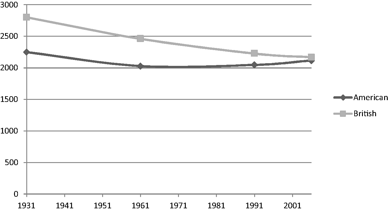
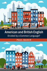
Figure 1.1 Frequencies of so
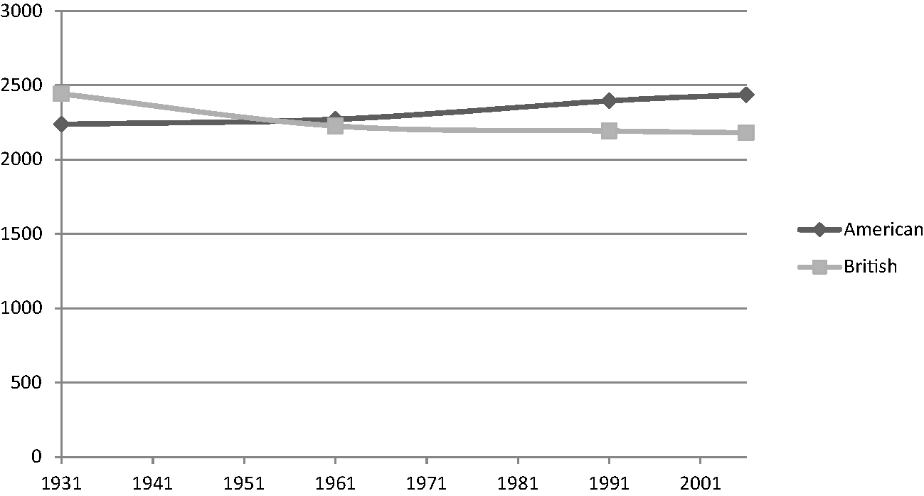
Figure 1.2 Frequencies of who
Figure 1.3 Frequencies of didn't
First, Figure 1.1 (so) indicates a change that is more marked in British English than American English. British English shows a continuous decline across the four sampling points, whereas the change is not so clear for American English where the frequencies first go down, then up again. This could be noted as a case of regionally specific change, but we could also characterise it as convergent change in that each subsequent sampling point has the two varieties showing closer frequencies than the one before. By the last sampling point (2006), the frequencies are almost identical (different starting points and similar end points). Throughout the book I represent frequencies as graphs like the one in Figure 1.1, although I sometimes also employ a notation system which puts the frequencies of four corpora from the same variety in square brackets, listed in chronological order. So for Figure 1.1 the American frequencies over time can be represented as [2250, 2029, 2047, 2117] while the British ones are [2801, 2460, 2226, 2168].
Figure 1.2 (who), shows contrary change (American English has an increasing use of who while British English shows decreasing use), and this could also be noted as a case of divergent change, in that the frequencies are further away from each other in 2006 compared to the starting point of 1931.
Finally, Figure 1.3 (didn't) shows a clear case of parallel change, with both varieties showing change in the same direction (upwards). However, the figure also shows the follow-my-leader pattern, with the frequency for American English always higher at each point than that of British English. Use of didn't clearly appears to be rising over time but this process appears to be more advanced for American English than it is for British English. As Leech et al (Reference Leech, Hundt, Mair and Smith2009: 43) note, this is ‘probably the most interesting pattern’, and it is one that I focus on most, as one of the motivations for writing this book is to carry out a fuller exploration of the extent to which American English is ‘leading’ linguistic change. However, divergent change (although quite rare in reality) is of interest too, along with convergent change, which functions as a related form of ‘follow my leader’.
Knowing whether a word shows divergent, convergent, parallel or regionally specific change is useful but it does not tell us much more than that. A more interesting question is why is that particular change happening? Presently I will explain how we address that question by considering different types of context relating to a word, but before I do that it is worth taking a slight diversion in order to explain how I identified the different types of change in the first place.
At the beginning of this research project I consulted with statisticians, hoping to identify a single ‘magic test’ which could be carried out on any word (or other feature) in all eight corpora and would reveal what is happening to that word. However, due to the fact that I wanted to make different sorts of comparisons and was asking different questions of the data, it transpired that using a combination of tests would be more effective. I have thus relied on three different procedures, which are summarised below but will also be described again where relevant in the coming chapters.
Keywords (and Key Clusters, Letter Sequences and Tags)
As briefly mentioned above, a keyword is a word which occurs relatively more often in one corpus when compared against another. A statistical test is used in order to identify the extent of the difference in frequency of the word between the two corpora. This test uses the frequencies of the word in each corpus as well as taking into account the total number of words in both. Utilised by Mike Scott in WordSmith Tools, keywords are one of the most popularly used corpus methods, and are now found in many other corpus analysis software packages. Ideas about the best statistical way of calculating keywords have changed over the years. The chi square statistic was initially popular (see Hofland and Johansson Reference Hofland and Johansson1982), but was criticised for producing too many keywords (Kilgarriff Reference Kilgarriff, Evett and Rose1996a, Reference Kilgarriff1996b, Reference Kilgarriff1997) and being ineffective on low-frequency data (Butler Reference Butler1985). It was also seen as problematic in that it assumes a normal frequency distribution which is not the case for language data (Dunning Reference Dunning1993). Dunning (Reference Dunning1993) suggested the log-likelihood test as an alternative and this is currently a measure that is used in many corpus analysis tools. It is a hypothesis-testing measure, which tells us the likelihood that a word actually is a keyword, but does not say anything about how strong the frequency difference is between the two corpora. More recently, Gabrielatos and Marchi (Reference Gabrielatos and Marchi2012) have argued against such hypothesis-testing measures as they do not measure the strength or ‘effect size’ of a difference. They have suggested a measure called %DIFF, while Andrew HardieFootnote 6 has proposed an effect-size measure called log-ratio, which has been implemented in the online tool CQPweb. In this book I employ the more widely known log-likelihood measure as the main way of identifying keywords, although I also apply a second filter based on the log-ratio score to remove a small number of items which do not show a strong difference.
To illustrate how the keywords measure works, let's look at the case of the word today. Table 1.3 shows the frequency of this word in all eight of the corpora.
Table 1.3 Frequencies of the word today in the eight Brown corpora
| British English | American English | |
|---|---|---|
| 1931 | 14 | 325 |
| 1961 | 300 | 324 |
| 1991/2 | 267 | 287 |
| 2006 | 270 | 278 |
We have eight corpora and thus eight frequencies in this table, but a keywords measure only involves a comparison of two corpora. So we need to take each row of the table separately, in effect carrying out four keyword tests on each word we look at. So taking the top row of numbers first, for the period 1931, we can compare the frequency of 14 (for British English)Footnote 7 with the frequency of 325 (for American English). In order to do a keyword comparison we also need to know the total size of each corpus (1 million words). If we enter all these numbers into a log-likelihood calculatorFootnote 8 it produces a log-likelihood score of 353.31. The higher the score, the greater the confidence that a word is a keyword. Taking a cut-off of 50,Footnote 9 we can say that for the two 1931 corpora, today is a keyword (being key in American English). How about the other periods? For the 1961 frequencies, the log-likelihood score is only 0.92. For the 1990s corpora it is 0.72 and for the 2006 corpora it is 0.12. These three numbers are all well below the cut-off point of 50, so for the purposes of this book I do not consider them to identify keywords. The word today can be called a keyword, but only in 1931, where it is much more frequent in American English. For the other three sampling points, there is not enough difference in its frequency between American and British English for it to be key.
So I have used the keywords technique to compare which words are especially frequent in one variety compared to another at different points in time. For each word this was achieved by carrying out four sets of keywords comparisons, first comparing the two 1930s corpora against each other, then the 1960s corpora, then the 1990s corpora, and finally the 2000s corpora. This procedure allows me to focus on long-standing differences between the two varieties. So for example, the word attorney is key at all four time points for American English – a consistent and long-lasting difference, making it a distinctly American word. By this I do not mean that it is never used in British English – but that it is statistically significantly more likely to be key in American English. On the other hand, amongst is only key for British English in the 1930s. After that, its frequency becomes more similar in both varieties. However, the finding for amongst raises a question – has amongst stopped being key because British writers are no longer using it very much so its frequency has fallen to American levels, or is it because Americans are using it more often (or has there been a kind of compromise where there is a decrease in British uses alongside an increase in American cases)? The keywords technique alone cannot answer this, so I have employed a second measure called the Coefficient of Variation.
The Coefficient of Variation
In order to examine change over time across a single variety, the Coefficient of Variation works well. While the keywords technique only involves a comparison of two corpora, the Coefficient of Variation (CV) is more effective when considering multiple measurements. Put simply, it gives a value based on the amount of variation across a set of points. A large value means that the points are widely distributed (and thus it suggests that a feature is changing quite a lot over time), while a small value indicates stability in use of that feature over time. The CV is calculated by taking the standard deviation of a set of values and then dividing it by the mean of that set of values (which acts as a way of cancelling out the effect of overall frequency sizeFootnote 10). The CV can thus be calculated on all words in the four American (or four British) corpora, and the words with the highest CVs will be those which show the most change over time. Obviously, not all of these words will show a straightforward decrease or increase over time; some will have a more snake-like pattern. As I am generally interested in cases of change which are ongoing, for most of the chapters (particularly in cases where a lot of such results were obtained) I usually filter out the snake-like cases.
The CV helps me to spot cases of words (or other phenomena) in a variety which show the most impressive growth or decline over time. By comparing the CVs for the same word across the two varieties, I can see whether a word has shown a similarly impressive amount of change in both, neither or just one. For illustration purposes, let's take another example, this time for the word want. Table 1.4 shows the frequencies of want across the eight corpora.
Table 1.4 Frequencies of the word want in the eight Brown corpora
| British English | American English | |
|---|---|---|
| 1931 | 343 | 254 |
| 1961 | 371 | 329 |
| 1991/2 | 438 | 509 |
| 2006 | 473 | 619 |
While the keywords comparison involved taking one row at a time, the CV involves taking one column at a time. So first we take the four frequencies for British English: [343, 371, 438, 473]. The CV is the standard deviation of these four numbers divided by the mean which works out as 59.74 divided by 406.2 giving 0.147. We then multiply this by 100 to get 14.7. Normally, the CV is between 0 and 100 – the higher the number, the greater the difference between the frequencies. A CV of 14.7 might not appear very large, so to make sense of it I have compared it against the CVs of all the other words in the corpus. In fact, for British English, want has a relatively low CV. If we order all the words in the British corpus according to their CV score, want comes quite a long way down the list. It is definitely not one of the top 20 words in terms of CV. On the other hand, when we look at the last column of Table 1.4, for American English [254, 329, 509, 619], the CV comes to 38.19. This is one of the highest CVs of all the words in American English (it is in the top 20 words which show a constantly increasing frequency over time). We would thus devote some attention to what is happening to the word want in American English, but might be less interested in it for British English.
Correlation
A keyword comparison takes two corpora at a time, the CV takes four at a time, while the final measure I have used is correlation, which takes all eight corpora into account. A correlation measure takes two lines drawn on a graph (such as in Figure 1.1) and produces a number (between −1 and +1) based on the extent to which the lines are moving in the same direction. A number close to +1 indicates that the lines are parallel to each other (as with the case of didn't in Figure 1.3 above), whereas one close to −1 indicates that the lines are moving in opposite directions (as with who in Figure 1.2). The frequencies of who are shown in Table 1.5.
Table 1.5 Frequencies of the word who in the eight Brown corpora
| British English | American English | |
|---|---|---|
| 1931 | 2451 | 2240 |
| 1961 | 2236 | 2280 |
| 1991/2 | 2209 | 2414 |
| 2006 | 2193 | 2437 |
The frequencies in Table 1.5 show that for British English, who has slowly but consistently decreased across the four time periods, whereas for American English, who has increased. When these eight frequencies are entered into two columns in an Excel spreadsheet and the CORREL measure is applied to them, we get a correlation score of −0.87 – one of the lowest scores of negative correlation for all the words examined.
Importantly, the correlation statistic does not tell us what direction the lines are moving in, or whether either of the lines show dramatic changes or just slight ones, nor do they tell us whether one language variety has a greater use of a feature compared to the other, but if we combine the correlation measure with the keywords and CV analyses, we can build a better profile of a feature's behaviour. The CV and correlation measures were calculated using Microsoft Excel, whereas WordSmith 5 was used to calculate keywords (while Wmatrix calculated key part of speech and semantic tags). These three methods are summarised again in the relevant chapters that they appear in.
Having just mentioned some of the tools used to carry out the analysis, it is worth elaborating on the ways that they were implemented in a little more detail. An important aspect of the corpus linguistics method is its replication, of which transparency should feature heavily. An ideal situation would be to have freely available corpora along with the tool(s) that were used to analyse them, so the same calculations can be carried out by others. In reality, the situation is not always so simple. In order to make the range of different comparisons of the eight corpora used in this book, no single tool was up to the task on its own. I thus employed five software packages, as shown in Table 1.6.
Table 1.6 Tools used for analysis
Interpreting and Explaining: Going from the Quantitative to the Qualitative
Considering that we can use keywords, the CV and correlation measures to identify words, sequences or tags which show a major difference between two varieties or a large pattern of change over time, what do we do with that information? Simply presenting our statistical findings in tables only counts as an early stage in our analysis. We then need to go on to interpret and explain our results. So we should ask the following questions: what is a particular word, sequence or tag used to achieve in the eight corpora, what contexts does it occur in and is this the same or different when we compare the corpora together?
To answer these questions we need to explore the language in the corpora in more detail, starting from a consideration of the contexts that a linguistic item appears in. For example, we might want to take into account whether an item is distributed evenly across an entire corpus, or whether it only occurs in a small number of texts or text types. If it is relatively frequent but only appears in a handful of files, we may want to play down its significance as its high frequency is probably due a few atypical files being included in the corpus, rather than telling us anything more generalisable about that time period. On the other hand, if an item appears in numerous files across a small number of registers (for example, it may mostly occur in several files containing fiction), then that is worth taking into account. Where it is relevant, I have tried to incorporate a consideration of distribution of an item across a corpus.
A second way that we can consider context is to examine how an item is embedded within the language of a particular text. For example, we could take into account collocates – words which appear next to or near one another a great deal, more than would be expected if all the words in a corpus were jumbled up in a random order. A word's collocates help us to understand its meaning. For example, in one corpus the word bank may collocate with river, reeds, water, vole and otter, while in another the same word could collocate with money, lend, city, loan and mortgage. The different sets of collocates help us to understand that the word has a different meaning in the two corpora.
Collocates can give a quick way of immediately deriving a word's meaning and context of use, and can be especially useful if we are working with high-frequency words. However, another approach involves reading the texts in detail via a technique called concordancing. A concordance is a table which shows all of the citations of a particular word with several words of context either side. Table 1.7 shows a concordance of the word bank for the 1931 American English corpus. As there were 157 occurrences of this word in that corpus, to save space I have only included 10 examples, taken at random.
Table 1.7 Sample concordance lines of bank from 1931 American English
| 1 | wading as fast as he could toward the opposite | bank | Fate laughed, a dangerous, wicked laugh, |
| 2 | present conditions in handling the details of | bank | without adding further to his burdens, |
| 3 | for a short way and then crossed to | bank | of the North Platte and to follow it to Fort |
| 4 | This is a splendid tribute to the character of | bank | management and to the efficiency of |
| 5 | When it was unloaded in the N. W. National | Bank | , it created comment and the officers were |
| 6 | Their Position in Connection With | Bank | Debts Defined by Law. To the Editor of The |
| 7 | to the bend of the Platte and along its north | bank | to Fort William. There, crossing to the south |
| 8 | tackle the job next morning as soon as the | bank | was open. Breaking into and robbing the |
| 9 | year of 1928. Mr. Ivey further stated that the | bank | 's conservative policies had placed it in |
| 10 | that fully justifies the confidence reposed in | bank | management by depositors, customers and |
From reading this concordance table we can start to see the two senses of bank described above. Lines 1, 3 and 7 relate to the “river bank” meaning while 2, 4, 5, 6, 8, 9 and 10 relate to the ‘repository of money’ meaning. We might want to state that this indicates that in 1931 American English, bank was more likely to refer to money than rivers, but with only 10 cases considered, that doesn't leave much of a margin for error. Generally speaking, looking at a larger number of occurrences (say 100) would allow us to make a more confident claim.
Collocates and concordances are useful ways of interpreting the quantitative patterns in corpus data, but in themselves, they may not help to explain why a particular pattern exists. To do this we often need to take into account sources of context from outside the corpus, instead looking at information about the society that the corpus came from. This can involve bringing together different types of relevant data such as lifestyle and attitude surveys and consideration of political, economic and social movements and the impact of important events. For example, in Chapter 7 I found that in all the American corpora, at every time period there are significantly higher references to words relating to law and order than in their respective British corpora. In order to try to explain this finding I carried out some contextual research looking at how the two cultures relate to the concept of law and order. I considered information such as claims about the extent to which each country is litigious, the number of lawyers, and the numbers and types of people in prison in each country (and the reasons that people have given for this), and the extent to which words referring to law and order were used literally or metaphorically in all the corpora. This type of analysis goes beyond frequency data, then, to position findings within different types of context.
To get a fuller perspective, once I have a good understanding of a pattern around a word, I try to consider how that word relates to other words. For example, with the word who, is its change related in some way to similar words which have a similar function (such as whom)? Can certain words be grouped together as showing a similar pattern and is their increase or decrease relating to a larger trend? Studies of linguistic change have already identified several trends such as grammaticalisation, informalisation, densification and democratisation, which are discussed throughout the book where appropriate. As an illustration of a type of trend which involves many words, the following section looks at word and sentence lengths in the eight corpora, relating this to the concept of densification.
Changing Word and Sentence Lengths
An initial way of thinking about the eight corpora involves looking at the length and variety of words and sentences. Figures 1.4–1.6 present three calculations for the corpora. First the mean word length is based on the number of letters in each word (Figure 1.4). Second, the mean sentence length is based on the number of words on average in each corpus (Figure 1.5). Finally, the standardised type token ratio (Figure 1.6) is slightly more complex to explain. Each corpus is made of types and tokens. A token is simply any wordFootnote 11, while types are unique words. So for example, the word dragon occurs seven times in the American 2006 corpus. This counts as seven word tokens, but only one word type. The type/token ratio is simply the number of types in a corpus divided by the number of tokens (and expressed as a percentage). This is a useful measure in that it shows the amount of lexical repetition in a corpus. A low type/token ratio (close to zero) indicates that a corpus has few types of words in it, perhaps because it is sampled from a fairly narrow genre of language, or in some cases, because it contains quite a simple use of language. On the other hand, a high type/token ratio indicates a much more lexically diverse use of language with many different words in a corpus. A problem with calculating the type/token ratio, however, is that it tends to inversely correlate with corpus size. This is due to the fact that very frequent words like the, it and that will have an increasingly skewing effect on the type-token ratio as corpus size increases. In order to account for this, type-token ratios are usually standardised by calculating separate ratios for each 1000-word chunk of text in a corpus and then working out the mean of all these ratios.
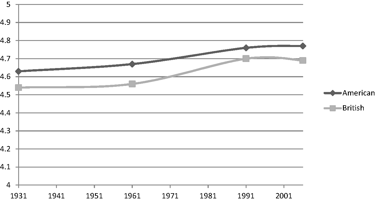
Figure 1.4 Mean word lengths
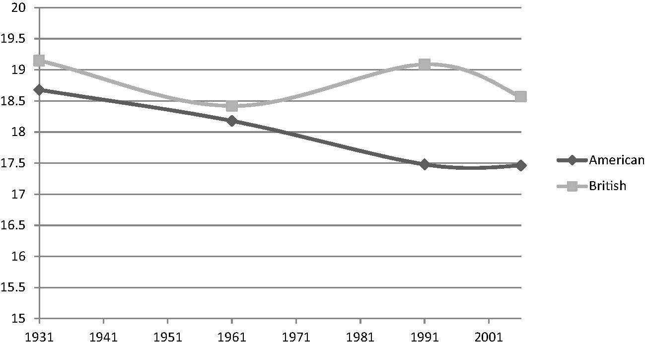
Figure 1.5 Mean sentence lengths
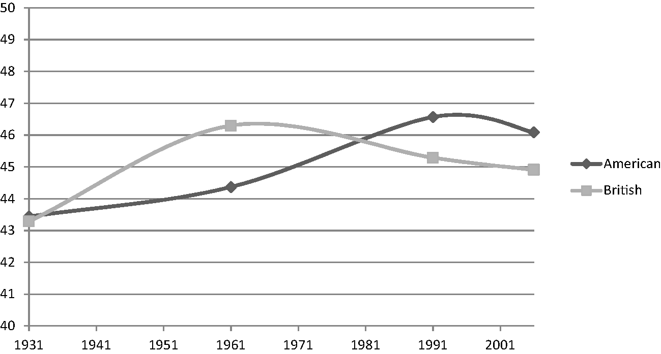
Figure 1.6 Standardised type token ratios
Figure 1.4 indicates that generally, mean word length has increased between 1931 and 2006, with each measurement larger than the one before. This is the case for both varieties, although the pattern looks to be more advanced for American English. The lines between 1991/2 and 2006 are more horizontal, which may indicate that the trend is beginning to level off, although more collection points would be needed to confirm this.
The reverse pattern is the case for mean sentence length, with sentences appearing to contain fewer words over time (Figure 1.5). For American English, on average a sentence in 2006 is about one word shorter than one written in 1931. British English has a more snake-like pattern, although still shows a downwards trend over time, just not as pronounced compared to American English. As with word length, it is American English which appears to be ahead of the trend.
As for the standardised type token ratio (Figure 1.6) which measures lexical diversity, neither line is straight, but there does appear to be an increase over time in both varieties. It is difficult to say that there is a clear pattern though, or that one variety is ‘in the lead’.
If these trends were to continue in future, we would expect to see a more diverse use of language (larger vocabularies) but one in which information is more densely packed with longer words and shorter sentences – a trend towards ‘densification’ in other words. In Chapter 9 I offer a few tentative suggestions based on the findings across the book about what the coming decades may hold if certain trends continue. However, predicting the future is difficult, and we must take care not to assume a ‘business as usual’ scenario where trends seen now simply continue along the same lines. For example, the spread of the Internet and computer-mediated communication from the early 1990s onwards has impacted on written language in numerous ways that could not have been predicted in the 1930s. Similarly, it is difficult to imagine how future technology or world events might alter language use by the end of the twenty-first century.
Overview of the Book
This chapter ends with an overview of the remaining chapters of the book. Each analysis chapter examines change and variation at a different linguistic level. So Chapter 2 begins with a brief examination of Noah Webster's spelling reforms of American English in the early nineteenth century, as a way of distinguishing and solidifying American identity from Britain, particularly in the aftermath of the War of Independence. I then examine and compare changing frequencies of spelling differences between British and American English, e.g. pairs like color/colour, center/centre and realize/realise. The chapter ends with a discussion of influences on spelling choice, including the use of spell-checkers in word processors, editorial decisions, and the internationalisation of news via the Internet.
Having considered spelling, Chapter 3 moves on to examine change and variation around the use of sequences of letters within words, which indirectly allows us to analyse affixation. After discussing the corpus-driven method for identifying and counting letter sequences (and picking out those which function as potential affixes across the eight corpora), I then describe how the Coefficient of Variation statistic (mentioned in the section above), was used in order to make comparisons which reveal the most (and least) dramatic changes over time. The remainder of the chapter focusses on a close analysis of 15 affixes, 8 which show very high amount of change over time in either American or British English (or both), and 7 which show much more stable frequencies over time in one or both language varieties. With each of the affixes I carry out qualitative analyses which take into account the types and numbers of words which a particular affix is most likely to occur in, the registers it is most likely associated with and whether the patterns of change or stability surrounding the affix can be linked to societal factors.
While Chapters 2 and 3 consider variation within words, the next two chapters look at words themselves. Chapter 4 is the first of two lexical chapters, each of which takes a somewhat different perspective. Focussing on high-frequency phenomena (around 400 words which occur at least 1000 times across the four British or four American corpora), I look at keywords and words with a high Coefficient of Variation in order to identify the words which show the most variation and/or change over time. The analysis concentrates on sets of words which contribute towards three larger-scale trends in the development of English – densification, democratisation and informalisation, while it ends with a discussion of the words who and say which show negative correlation for the two varieties, as well as considering two- and three-word clusters (sequences of words) which have high CVs in one or both varieties.
Following this, Chapter 5 looks at a set of words which have lower frequencies to examine the extent to which the two varieties have a distinct vocabulary (this chapter covering perhaps what most people would identify as differences between American and British English). Similar to Chapter 2 which used keywords to elicit spelling differences, this chapter turns again to keywords to identify lexical variation such as gasoline versus petrol or courgette versus zucchini. After a discussion of the pitfalls of working with less frequent phenomena in small corpora (and dangers in assuming that such words are always direct equivalents), I examine words based on the categories of transport, the monarchy, politics and law, business and economics, people, and entertainment and leisure.
Moving beyond words, Chapters 6 and 7 use automatic tagging to group words into categories, taking a similar structure which uses keywords, the CV and correlations. Chapter 6 uses versions of the Brown family where words have been tagged for part of speech categories (such as singular common noun and adverb of degree), focussing on change and variation in grammatical phenomena. The resulting analysis leads to discussion of features which include the passive voice, modality, relative clauses, noun compounds, titles and genitives, drawing again on the concepts of densification, democratisation and informalisation as large-scale explanatory trends.
In Chapter 7 I tag the corpora again, this time using a set of several hundred semantic tags which are based around meaning as opposed to grammatical function. The aim of this chapter is to understand what British and American people write about, as opposed to how they write. For example, to what extent is America a land of ‘guns, god and corporate gurus’ (as the title of James Laxer's Reference Laxer2001 book claims)? Thus, despite using a semantic tagset, this chapter actually uncovers cultural differences between the two varieties, with the resulting analyses being focussed around categories such as war and law, social interactions and people, technology and media, and ideas and concepts. More than the previous chapters, this chapter requires the application of contextual information about the societies and time periods in which the corpora were created in order to interpret and explain some of the trends found.
Chapter 8 takes a different approach to the previous chapters in that it is more corpus-based, rather than corpus-driven. In advance of the analysis in this chapter I selected a set of phenomena which I hypothesised might reveal differences over time or between the two varieties, partly based on the results of the analyses of Chapters 2–7. These phenomena included swearing and profanity, markers of identity (gender, sexuality and race), and discourse markers, some of which can be used to express stance or function as organisers (such as nevertheless and on the other hand), others which are much more commonly associated with spoken language and have pragmatic or politeness functions, such as please, thank you and sorry.
Finally, in Chapter 9 I summarise the main findings from the previous analysis chapters and offer a few cautious projections about the future of English in the light of a globalised, connected planet, focussing on the effects of computer-mediated communication, as well as considering the extent to which British English is actually undergoing Americanisation. The book ends with a discussion of some of the possible directions that research in corpus studies of language variation and change can take, along with some critical reflections on the method taken.


